visitor ]Kavli Institute for Theoretical Physics, Santa Barbara.
also at ]Jawaharlal Nehru Centre For Advanced Scientific Research, Jakkur, Bangalore, India

Dynamic Multiscaling in Two-dimensional Fluid Turbulence

Abstract

We obtain, by extensive direct numerical simulations, time-dependent and equal-time structure functions for the vorticity, in both quasi-Lagrangian and Eulerian frames, for the direct-cascade regime in two-dimensional fluid turbulence with air-drag-induced friction. We show that different ways of extracting time scales from these time-dependent structure functions lead to different dynamic-multiscaling exponents, which are related to equal-time multiscaling exponents by different classes of bridge relations; for a representative value of the friction we verify that, given our error bars, these bridge relations hold.

The scaling properties of both equal-time and time-dependent correlation functions close to a critical point, say in a spin system, have been understood well for nearly four decades *[See; e.g.; ][andreferencestherein]Cha+Lub98; hoh+hal77 . By contrast, the development of a similar understanding of the multiscaling properties of equal-time and time-dependent structure functions in the inertial range in fluid turbulence still remains a major challenge for it requires interdisciplinary studies that must use ideas both from nonequilibrium statistical mechanics and turbulence kol41 ; Fri96 ; lvo+pod+pro97 ; bif+bof+cel+tos99 ; kan+ish+got99 ; mit+pan03 ; mit+pan04 ; mit+pan05 ; ray+mit+pan08 ; pan+ray+mit08 . We develop here a complete characterization of the rich multiscaling properties of time-dependent vorticity structure functions for the direct-cascade regime of two-dimensional (2D) turbulence in fluid films with friction, which we study via a direct numerical simulation (DNS). Such a characterization has not been possible hitherto because it requires very long temporal averaging to obtain good statistics for quasi-Lagrangian structure functions bel+lvo87 , which are considerably more complicated than their conventional, Eulerian counterparts as we show below. Our DNS study yields a variety of interesting results that we summarize informally before providing technical details and precise definitions: (a) We calculate equal-time and time-dependent vorticity structure functions in Eulerian and quasi-Lagrangian frames bel+lvo87 . (b) We then show how to extract an infinite number of different time scales from such time-dependent structure functions. (c) Next we present generalizations of the dynamic-scaling Ansatz, first used in the context of critical phenomena hoh+hal77 to relate a diverging relaxation time $\tau$ to a diverging correlation length $\xi$ via $\tau\sim\xi^{z}$, where $z$ is the dynamic-scaling exponent. These generalizations yield, in turn, an infinity of dynamic-multiscaling exponents lvo+pod+pro97 ; bif+bof+cel+tos99 ; mit+pan03 ; mit+pan04 ; mit+pan05 ; ray+mit+pan08 ; pan+ray+mit08 . (d) A suitable extension of the multifractal formalism Fri96 , which provides a rationalization of the multiscaling of equal-time structure functions in turbulence, yields linear bridge relations between dynamic-multiscaling exponents and their equal-time counterparts lvo+pod+pro97 ; bif+bof+cel+tos99 ; mit+pan03 ; mit+pan04 ; mit+pan05 ; ray+mit+pan08 ; pan+ray+mit08 ; our study provides numerical evidence in support of such bridge relations.

The statistical properties of fully developed, homogeneous, isotropic turbulence are characterized, inter alia, by the equal-time, order-$p$, longitudinal-velocity structure function ${\mathcal{S}}_{p}(r)\equiv\langle[\delta u_{\parallel}(r,t)]^{p}\rangle$, where $\delta u_{\parallel}(r,t)\equiv[{\bf u}({\bf x}+{\bf r},t)-{\bf u}({\bf x},t)\cdot{\bf r}/r]$, ${\bf u}({\bf x},t)$ is the Eulerian velocity at point ${\bf x}$ and time $t$, and $r\equiv\mid{\bf r}\mid$. In the inertial range $\eta_{d}\ll r\ll L$, ${\mathcal{S}}_{p}(r)\sim r^{\zeta_{p}}$, where $\zeta_{p}$, $\eta_{d}$, and $L$, are, respectively, the equal-time exponent, the dissipation scale, and the forcing scale. The pioneering work kol41 of Kolmogorov (K41) predicts simple scaling with $\zeta_{p}^{K41}=p/3$ for three-dimensional (3D) homogeneous, isotropic fluid turbulence. However, experiments and numerical simulations show marked deviations from K41 scaling, especially for $p\geq 4$, with $\zeta_{p}$ a nonlinear, convex function of $p$; thus, we have multiscaling of equal-time velocity structure functions. To examine dynamic multiscaling, we must obtain the order-$p$, time-dependent structure functions ${\mathcal{F}}_{p}(r,t)$, which we define precisely below, extract from these the time scales $\tau_{p}(r)$, and thence the dynamic-multiscaling exponents $z_{p}$ via dynamic-multiscaling Ansätze like $\tau_{p}(r)\sim r^{z_{p}}$. This task is considerably more complicated than its analog for the determination of the equal-time multiscaling exponents $\zeta_{p}$ lvo+pod+pro97 ; bif+bof+cel+tos99 ; kan+ish+got99 ; mit+pan03 ; mit+pan04 ; mit+pan05 ; ray+mit+pan08 ; pan+ray+mit08 for the following two reasons: (I) In the conventional Eulerian description, the sweeping effect, whereby large eddies drive all smaller ones directly, relates spatial separations $r$ and temporal separations $t$ linearly via the mean-flow velocity, whence we get trivial dynamic scaling with $z_{p}=1$, for all $p$. A quasi-Lagrangian description lvo+pod+pro97 ; bel+lvo87 eliminates sweeping effects so we calculate time-dependent, quasi-Lagrangian vorticity structure functions from our DNS. (II) Such time-dependent structure functions, even for a fixed order $p$, do not collapse onto a scaling function, with a unique, order-$p$, dynamic exponent. Hence, even for a fixed order $p$, there is an infinity of dynamic-multiscaling exponents lvo+pod+pro97 ; bif+bof+cel+tos99 ; mit+pan03 ; mit+pan04 ; mit+pan05 ; ray+mit+pan08 ; pan+ray+mit08 ; roughly speaking, to specify the dynamics of an eddy of a given length scale, we require this infinity of exponents.

Statistically steady fluid turbulence is very different in 3D and 2D; the former exhibits a direct cascade of energy whereas the latter shows an inverse cascade of kinetic energy from the energy-injection scale to larger length scales and a direct cascade in which the enstrophy goes towards small length scales kraic67 ; *lei68; *bat69; in many physical realizations of 2D turbulence, there is an air-drag-induced friction. In this direct-cascade regime, velocity structure functions show simple scaling but their vorticity counterparts exhibit multiscaling bof+cel+mus+ver02 ; tsa+ott+ant+guz05 ; per+pan09 , with exponents that depend on the friction. Time-dependent structure functions have not been studied in 2D fluid turbulence; the elucidation of the dynamic multiscaling of these structure functions, which we present here, is an important step in the systematization of such multiscaling in turbulence.

We numerically solve the forced, incompressible, 2D Navier-Stokes (2DNS) equation with air-drag-induced friction, in the vorticity($\omega)$–stream-function($\psi)$ representation with periodic boundary conditions:

$$\partial_{t}\omega-J(\psi,\omega)=\nu\nabla^{2}\omega-\mu\omega+f,$$ (1)

where $\nabla^{2}\psi=\omega$, $J(\psi,\omega)\equiv(\partial_{x}\psi)(\partial_{y}\omega)-(\partial_{x}\omega)(\partial_{y}\psi)$, and the velocity ${\bf u}\equiv(-\partial_{y}\psi,\partial_{x}\psi)$. The coefficient of friction is $\mu$ and $f$ is the external force. We work with both Eulerian and quasi-Lagrangian fields. The latter are defined with respect to a Lagrangian particle, which was at the point $\bm{\xi}_{\rm 0}$ at time $t_{0}$, and is at the position $\bm{\xi}(t|\bm{\xi}_{\rm 0},t_{0})$ at time $t$, such that $d\bm{\xi}(t|\bm{\xi}_{\rm 0},t_{0})/dt={\bf u}[\bm{\xi}(t|\bm{\xi}_{\rm 0},t_{0}),t]$, where ${\bf u}$ is the Eulerian velocity. The quasi-Lagrangian velocity field ${\bf u}^{\rm QL}$ is defined bel+lvo87 as follows:

$${\bf u}^{\rm QL}({\bf x},t|\bm{\xi}_{\rm 0},t_{0})\equiv{\bf u}[{\bf x}+\bm{\xi}(t|\bm{\xi}_{\rm 0},t_{0}),t];$$ (2)

likewise, we can define the quasi-Lagrangian vorticity field $\omega^{\rm QL}$ in terms of the Eulerian $\omega$. To obtain this quasi-Lagrangian field we use an algorithm developed in Ref. Mit05 , described briefly in the Supplementary Material.

To integrate the Navier-Stokes equations we use a pseudo-spectral method with the $2/3$ rule for the removal of aliasing errors per+pan09 and a second-order Runge-Kutta scheme for time marching with a time step $\delta t=10^{-3}$. We force the fluid deterministically on the second shell in Fourier space. And we use $\mu=0.1$, $\nu=10^{-5}$, and $N=2048^{2}$ collocation points  We obtain a turbulent but statistically steady state with a Taylor microscale $\lambda\simeq 0.2$, Taylor-microscale Reynolds number $Re_{\lambda}\simeq 1400$, and a box-size eddy-turn-over time $\tau_{{\rm eddy}}\simeq 8$. We remove the effects of transients by discarding data upto time $\lesssim 80\tau_{{\rm eddy}}$. We then obtain data for averages of time-dependent structure functions for a duration of time $\simeq 100\tau_{{\rm eddy}}$. The energy spectrum averaged over the same time interval is shown in Fig. (1a).

The equal-time, order-$p$, vorticity structure functions we consider are ${\mathcal{S}}^{\phi}_{p}(r)\equiv\langle[\delta\omega^{\phi}(r,t)]^{p}\rangle\sim r^{\zeta^{\phi}_{p}}$, for $\eta_{d}\ll r\ll L$, where $\delta\omega^{\phi}(r,t)=[{\omega^{\phi}}({\bf x}+{\bf r},t)-{\omega^{\phi}}({\bf x},t)]$, the angular brackets denote an average over the nonequilibrium statistically steady state of the turbulent fluid, and the superscript $\phi$ is either ${\rm E}$, in the Eulerian case, or ${\rm QL}$, in the quasi-Lagrangian case; for notational convenience we do not include a subscript $\omega$ on $S_{p}^{\phi}$ and the multiscaling exponent $\zeta^{\phi}_{p}$. We assume isotropy here, but show below how to extract the isotropic parts of $S_{p}^{\phi}$ in a DNS. We also use the time-dependent, order-$p$ vorticity structure functions

$${\mathcal{F}}^{\phi}_{p}(r,\{t_{1},\ldots,t_{p}\})\equiv\langle[\delta\omega^{\phi}(r,t_{1})\ldots\delta\omega^{\phi}(r,t_{p})]\rangle;$$ (3)

here $t_{1},\ldots,t_{p}$ are $p$ different times; clearly, ${\mathcal{F}}^{\phi}_{p}(r,\{t_{1}=\ldots=t_{p}=0\})={\mathcal{S}}^{\phi}_{p}(r)$. We concentrate on the case $t_{1}=t_{2}=\ldots=t_{l}\equiv t$ and $t_{l+1}=t_{l+2}=\ldots=t_{p}=0$, with $l<p$, and, for simplicity, denote the resulting time-dependent structure function as ${\mathcal{F}}^{\phi}_{p}(r,t)$; shell-model studies mit+pan03 ; mit+pan04 have shown that the index $l$ does not affect dynamic-multiscaling exponents, so we suppress it henceforth. Given ${\mathcal{F}}^{\phi}_{p}(r,t)$, it is possible to extract a characteristic time scale $\tau_{p}(r)$ in many different ways. These time scales can, in turn, be used to extract the order-$p$ dynamic-multiscaling exponents $z_{p}$ via the dynamic-multiscaling Ansatz $\tau_{p}(r)\sim r^{z_{p}}$. If we obtain the order-$p$, degree-$M$, integral time scale

$${\cal T}^{I,\phi}_{p,M}(r)\equiv\biggl{[}\frac{1}{{\mathcal{S}}^{\phi}_{p}(r)}\int_{0}^{\infty}{\mathcal{F}}^{\phi}_{p}(r,t)t^{(M-1)}dt\biggl{]}^{(1/M)},$$ (4)

we can use it to extract the integral dynamic-multiscaling exponent $z^{I,\phi}_{p,M}$ from the relation ${\cal T}^{I,\phi}_{p,M}\sim r^{z^{I,\phi}_{p,M}}$. Similarly, from the order-$p$, degree-$M$, derivative time scale

$${\cal T}^{D,\phi}_{p,M}\equiv\biggl{[}\frac{1}{{\mathcal{S}}^{\phi}_{p}(r)}\frac{\partial^{M}}{\partial t^{M}}{\mathcal{F}}^{\phi}_{p}(r,t)\biggl{|}_{t=0}\biggl{]}^{(-1/M)},$$ (5)

we obtain the derivative dynamic-multiscaling exponent $z^{D,\phi}_{p,M}$ via the relation ${\cal T}^{D,\phi}_{p,M}\sim r^{z^{D,\phi}_{p,M}}$.

Equal-time vorticity structure functions in 2D fluid turbulence with friction exhibit multiscaling in the direct cascade range bof+cel+mus+ver02 ; tsa+ott+ant+guz05 ; per+pan09 . For the case of 3D homogeneous, isotropic fluid turbulence, a generalization of the multifractal model Fri96 , which includes time-dependent velocity structure functions lvo+pod+pro97 ; mit+pan04 ; ray+mit+pan08 ; pan+ray+mit08 , yields linear bridge relations between the dynamic-multiscaling exponents and their equal-time counterparts. For the direct-cascade regime in our study, we replace velocity structure functions by vorticity structure functions and thus obtain the following bridge relations for time-dependent vorticity structure functions in 2D fluid turbulence with friction:

$$z^{I,\phi}_{p,M}=1+[\zeta^{\phi}_{p-M}-\zeta^{\phi}_{p}]/M;$$ (6)

$$z^{D,\phi}_{p,M}=1+[\zeta^{\phi}_{p}-\zeta^{\phi}_{p+M}]/M.$$ (7)

The vorticity field $\omega^{\phi}=\langle\omega^{\phi}\rangle+\omega^{\prime\phi}$ can be decomposed into the time-averaged mean flow $\langle\omega^{\phi}\rangle$ and the fluctuations $\omega^{\prime\phi}$ about it. To obtain good statistics for vorticity structure functions it is important to eliminate any anisotropy in the flow by subtracting out the mean flow from the field. Therefore, we redefine the order-$p$, equal-time structure function to be $S_{p}^{\phi}({\bf r_{c}},{\bf R})\equiv\langle|\omega^{\prime\phi}({\bf r_{c}}+{\bf R})-\omega^{\prime\phi}({\bf r_{c}})|^{p}\rangle$, where ${\bf R}$ has magnitude $R$ and ${\bf r_{c}}$ is an origin. We next use $S_{p}^{\phi}({\bf R})\equiv\langle S_{p}^{\phi}({\bf r_{c}},{\bf R})\rangle_{{\bf r_{c}}}$, where the subscript ${\bf r_{c}}$ denotes an average over the origin (we use ${\bf r_{c}}=(i,j),2\leq i,j\leq 5$). These averaged structure functions are isotropic, to a good approximation for small $R$, as can be seen from the illustrative pseudocolor plot of $S_{2}^{\rm QL}({\bf R})$ in Fig. (1a). The purely isotropic parts of such structure functions can be obtained per+pan09 ; bou+pro+sel05 via an integration over the angle $\theta$ that ${\bf R}$ makes with the $x$ axis, i.e., we calculate $S_{p}^{\phi}(R)\equiv\int_{0}^{2\pi}S_{p}^{\phi}({\bf R})d\theta$ and thence the equal-time multiscaling exponent $\zeta^{\phi}_{p}$, the slopes of the scaling ranges of log-log plots of $S_{p}^{\phi}(R)$ versus $R$. The mean of the local slopes $\xi_{p}\equiv d(\log S_{p}^{\phi})/d(\log R)$ in the scaling range yields the equal-time exponents; and their standard deviations give the error bars. The equal-time vorticity multiscaling exponents, with $1\leq p\leq 6$, are given for Eulerian and quasi-Lagrangian cases in columns 2 and 3, respectively, of Table 1; they are equal, within error bars, as can be seen most easily from their plots versus $p$ in Fig.(1c).

We obtain the isotropic part of ${\mathcal{F}}^{\phi}_{p}(R,t)$ in a similar manner. Equations (4) and (5) now yield the order-$p$, degree-$M$ integral and derivative time scales (see the Supplementary Material). Slopes of linear scaling ranges of log-log plots of ${\cal T}^{I,{\phi}}_{p,M}(R)$ versus $R$ yield the dynamic multiscaling exponent $z_{p,M}^{I,{\phi}}$. A representative plot for the quasi-Lagrangian case, $p=2$ and $M=1$, is given in Fig. (1 d); we fit over the range $-1.2<\log_{10}(r/L)<-0.55$ and obtain the local slopes $\chi_{p}$ with successive, nonoverlapping sets of 3 points each. The mean values of these slopes yield our dynamic-multiscaling exponents (column 5 in Table 1) and their standard deviations yield the error bars. We calculate the degree-$M$, order-$p$ derivative time exponents by using a sixth-order, finite-difference scheme to obtain ${\cal T}^{D,{\phi}}_{p,M}$ and thence the dynamic-multiscaling exponents $z_{p,M}^{D,{\phi}}$. Our results for the quasi-Lagrangian case with $M=2$ are given in column 7 of Table 1. We find, furthermore, that both the integral and derivative bridge relations (6) and (7) hold within our error bars, as shown for the representative values of $p$ and $M$ considered in Table 1 (compare columns 4 and 5 for the integral relation and columns 6 and 7 for the derivative relation). Note also that the values of the integral and the derivative dynamic-multiscaling exponents are markedly different from each other (compare columns 5 and 7 of Table 1).

The Eulerian structure functions ${\mathcal{F}}^{E}_{p}(R,t)$ also lead to nontrivial dynamic-multiscaling exponents, which are equal to their quasi-Lagrangian counterparts (see Supplementary Material). The reason for this initially surprising result is that, in 2D turbulence, the friction controls the size of the largest vortices, provides an infra-red cut-off at large length scales, and thus suppresses the sweeping effect. We have demonstrated this in the supplementary material. Had the sweeping effect not been suppressed, we would have obtained trivial dynamic scaling for the Eulerian case.

The calculation of dynamic-multiscaling exponents has been limited so far to shell models for 3D, homogeneous, isotropic fluid bif+bof+cel+tos99 ; mit+pan03 ; mit+pan04 ; ray+mit+pan08 ; pan+ray+mit08 and passive-scalar turbulence mit+pan05 . We have presented the first study of such dynamic multiscaling in the direct-cascade regime of 2D fluid turbulence with friction by calculating both quasi-Lagrangian and Eulerian structure functions. Our work brings out clearly the need for an infinity of time scales and associated exponents to characterize such multiscaling; and it verifies, within the accuracy of our numerical calculations, the linear bridge relations (6) and (7) for a representative value of $\mu$. We find that friction also suppresses sweeping effects so, with such friction, even Eulerian vorticity structure functions exhibit dynamic multiscaling with exponents that are consistent with their quasi-Lagrangian counterparts.

Experimental studies of Lagrangian quantities in turbulence have been increasing steadily over the past decade ott+man00 ; *por+vot+cra+ale+bod02; *mor+met+mic+pin01. We hope, therefore, that our work will encourage studies of dynamic multiscaling in turbulence. Furthermore, it will be interesting to check whether the time scales considered here can be related to the persistence time scales for 2D turbulence per+ray+mit+pan11 .

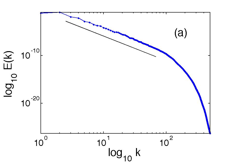
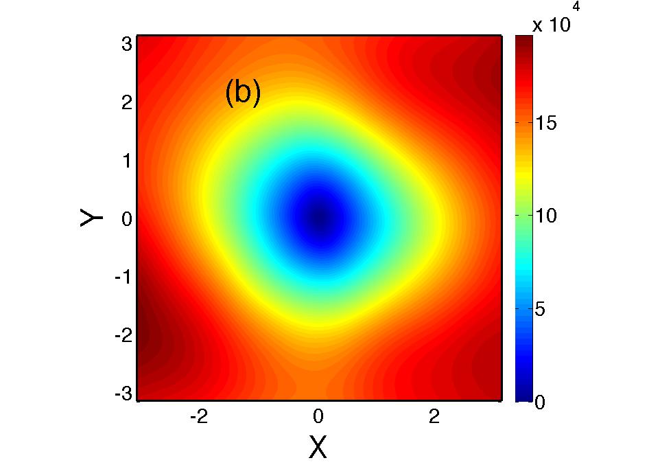
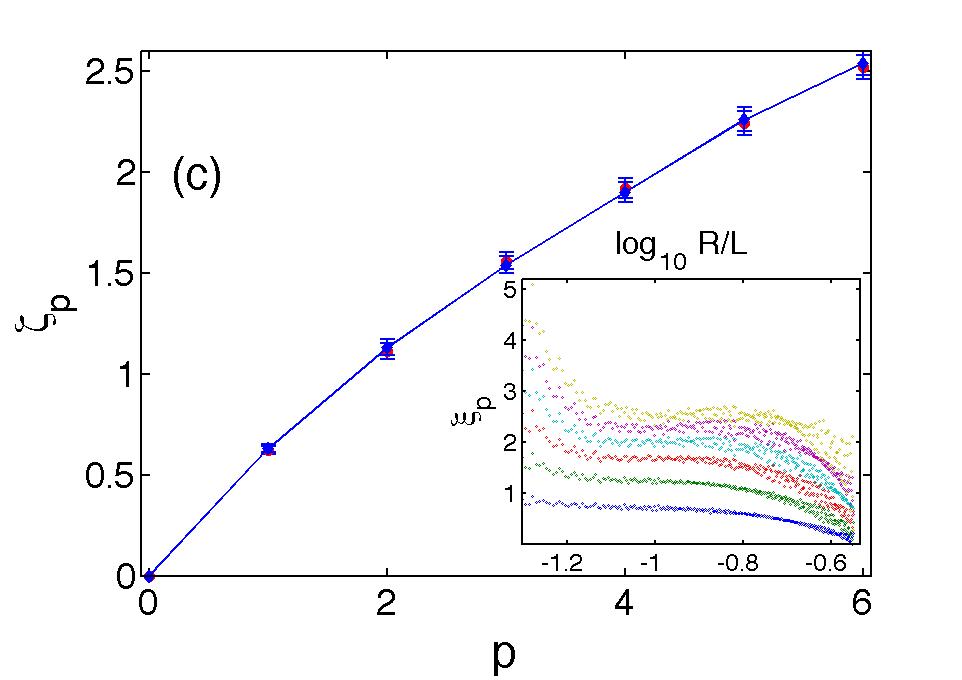
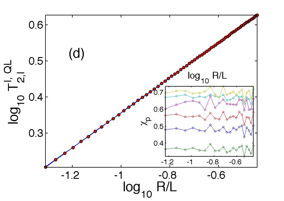
Figure 1: (Color online) (a) Log-log (base 10) plot of the energy spectrum $E(k)$ versus $k$. The black line with slope $-4.1$ is shown for reference. (b) Pseudocolor plot of the equal-time, quasi-Lagrangian, second-order vorticity structure function $S_{2}^{\rm QL}({\bf R})$ averaged over the origin ${\bf r_{c}}$ (we use ${\bf r_{c}}=(i,j),2\leq i,j\leq 5$); (c) plots of the equal-time, vorticity, multiscaling exponents $\zeta^{\phi}_{p}$ versus $p$ for Eulerian (red circles) and quasi-Lagrangian (blue diamonds) fields (error bars are comparable to the size of the symbols); the inset shows the local slopes $\xi_{p}$, obtained as defined in the text, versus the separation, from $p$ = 1 (bottom) to $p$ = 6 (top); (d) log-log (base 10) plot of the order-2, degree-1, integral time scale $T^{I,{\rm QL}}_{2,1}(R)$ versus the separation $R$ showing our data points (open red circles) and the best-fit line (full black) in the scaling range; the inset shows the local slopes $\chi_{p}$, obtained as defined in the text, versus the separation, from $p$ = 1 (bottom) to $p$ = 6 (top).

order$(p)$ $\zeta^{{\rm E}}_{p}$ $\zeta^{{\rm QL}}_{p}$ $z^{I,{\rm QL}}_{p,1}$[Eq.(6)] $z^{I,{\rm QL}}_{p,1}$ $z^{D,{\rm QL}}_{p,2}$[Eq.(7)] $z^{D,{\rm QL}}_{p,2}$ 1 0.62 $\pm$ 0.009 0.63 $\pm$ 0.008 0.366 $\pm$ 0.008 0.37 $\pm$ 0.02 0.55 $\pm$ 0.02 0.53 $\pm$ 0.02 2 1.13 $\pm$ 0.009 1.13 $\pm$ 0.008 0.50 $\pm$ 0.02 0.48 $\pm$ 0.01 0.62 $\pm$ 0.02 0.62 $\pm$ 0.2 3 1.561 $\pm$ 0.009 1.54 $\pm$ 0.01 0.59 $\pm$ 0.02 0.57 $\pm$ 0.01 0.64 $\pm$ 0.02 0.65 $\pm$ 0.01 4 1.92 $\pm$ 0.01 1.90 $\pm$ 0.01 0.64 $\pm$ 0.02 0.63 $\pm$ 0.01 0.68 $\pm$ 0.03 0.68 $\pm$ 0.01 5 2.24 $\pm$ 0.01 2.26 $\pm$ 0.01 0.64 $\pm$ 0.02 0.65 $\pm$ 0.02 0.70 $\pm$ 0.03 0.70 $\pm$ 0.02 6 2.52 $\pm$ 0.02 2.54 $\pm$ 0.02 0.72 $\pm$ 0.03 0.67 $\pm$ 0.02 0.71 $\pm$ 0.04 0.71 $\pm$ 0.03

Table 1: Order-$p$ (column 1); equal-time, Eulerian exponents $\zeta^{\rm E}_{p}$ (column 2); equal-time, quasi-Lagrangian exponents $\zeta^{\rm QL}_{p}$ (column 3); integral-scale, dynamic-multiscaling exponent $z^{I,{\rm QL}}_{p,1}$ (column 4) from the bridge relation and the values of $\zeta^{\rm QL}_{p}$ in column 3; $z^{I,{\rm QL}}_{p,1}$ from our calculations of time-dependent structure functions (column 5); the derivative-time exponents $z^{D,{\rm QL}}_{p,2}$ (column 6) from the bridge relation and the values of $\zeta^{\rm QL}_{p}$ in column 3; $z^{D,{\rm QL}}_{p,2}$ from our calculations of the time-dependent structure function (column 7). The error estimates are obtained as described in the text.

Appendix A Algorithm for obtaining quasi-Lagrangian fields in a pseudospectral simulation

To obtain a quasi-Lagrangian field from its Eulerian counterpart, we track a single Lagrangian particle by using a bilinear-interpolation method [17]. If we replace the Eulerian velocity in Eq. (2) by its Fourier-integral representation, we obtain

$${\bf u}^{\rm QL}({\bf x},t|\bm{\xi}_{\rm 0},t_{0})=\int{\bf{\hat{u}}}({\bf q},t)\exp[i{\bf q}\cdot({\bf x}+\bm{\xi}(t|\bm{\xi}_{\rm 0},t_{0}),t))]d{\bf q},$$

where ${\bf q}$ is the wave vector. In the pseudospectral algorithm we use to solve Eq. (1), the quasi-Lagrangian velocity is defined with respect to a Lagrangian particle, which was at the point $\bm{\xi}_{\rm 0}$ at time $t_{0}$, and is at the position $\bm{\xi}(t|\bm{\xi}_{\rm 0},t_{0})$ at time $t$, such that $d\bm{\xi}(t|\bm{\xi}_{\rm 0},t_{0})/dt={\bf u}[\bm{\xi}(t|\bm{\xi}_{\rm 0},t_{0}),t]$. We calculate ${\bf{\hat{u}}}({\bf q},t)$; thus, the Fourier integral above can be evaluated at each time step by an additional call to a fast-Fourier-Transform (FFT) subroutine. The additional computational cost of obtaining ${\bf u}^{\rm QL}$ at all collocation points is that of following a single Lagrangian particle and an additional FFT at each time step.

Appendix B Numerical determination of integral time scales from time-dependent structure functions

To extract the integral time scale, of degree $M$, from a time-dependent structure function, we have to evaluate the integral in Eq. (4) numerically. In practice, because of poor statistics at long times, we integrate from $t=0$ to $t=t_{*}$, where $t_{*}$ is the time at which ${\mathcal{F}}^{\phi}_{p}(R^{\prime},t)=\epsilon$; we choose $\epsilon=0.6$, but we have checked that our results do not change, within our error bars, for $0.5\leq\epsilon\leq 0.75$. This numerical integration is done by using the trapezoidal rule.

Appendix C Dynamic multiscaling for Eulerian structure functions

Equal-time Eulerian structure functions have been discussed in our paper above. To obtain time-dependent, Eulerian, vorticity structure functions we proceed as we did in the quasi-Lagrangian case. We obtain the required vorticity increments and from these the purely isotropic part of the time-dependent, order-$p$ structure function ${\mathcal{F}}^{\rm E}_{p}(R^{\prime},t)$. Equations (4) and (5) now yield the order-$p$, degree-$M$ integral and derivative Eulerian time scales. For the former we should integrate ${\mathcal{F}}^{\rm E}_{p}(R^{\prime},t)$ from $t=0$ to $t=\infty$; in practice, because of poor statistics at long times, we integrate from $t=0$ to $t=t_{*}$, where $t_{*}$ is the time at which ${\mathcal{F}}^{\rm E}_{p}(R^{\prime},t)=\epsilon$; we choose $\epsilon=0.6$, but we have checked that our results do not change, within our error bars, for $0.5\leq\epsilon\leq 0.75$. Slopes of linear scaling ranges of log-log plots of ${\cal T}^{I,{\rm E}}_{p,M}(R^{\prime})$ versus $R^{\prime}$ yield the dynamic multiscaling exponent $z_{p,1}^{I,{\rm E}}$. A representative plot for the Eulerian case, $p=2$, and $M=1$ is given in Fig. (2 a); we fit over the range $-1.2<\log_{10}(r/L)<-0.55$ and obtain the local slopes $\chi_{p}$ with successive, non-overlapping sets of 3 points each. The mean values of these slopes yield our dynamic-multiscaling exponents (column 4 in Table  2) and their standard deviations yield the error bars. We calculate the degree-$M$, order-$p$ derivative time exponents by using a sixth-order finite difference scheme to obtain ${\cal T}^{D,{\rm E}}_{p,M}$ and thence the dynamic-multiscaling exponents $z_{p,M}^{D,{\rm E}}$; data for the Eulerian case and the representative value $M=2$ are given in column 6 of Table 2. We find, furthermore, that both the integral and derivative bridge relations, Eq. (6), and Eq. (7). hold within our error bars, as shown for the representative values of $p$ and $M$ considered in Table 2 (compare columns 3 and 4 for the integral relation and columns 5 and 6 for the derivative relation). The values of the integral and the derivative dynamic-multiscaling exponents are markedly different from each other (compare columns 4 and 6 of Table 2) and the plots of these exponents versus $p$ in Fig. (2 b). In Fig. (2 c), we make the same comparison for the quasi-Lagrangian case. Furthermore, a comparison of the quasi-Lagrangian and Eulerian dynamic-multiscaling exponents given in Tables I in the original paper and Table 2, respectively, show that these are the same (within our error bars).

Appendix D Demonstration of Infra-red cutoff of the inverse cascade

We have shown that in two dimensional turbulence with friction, the Eulerian and the quasi–Lagrangian velocities have the same dynamical exponents. This is because the inverse cascade has a friction–dependent infra-red cutoff.

To illustrate the development of this cutoff scale, we have carried out DNS studies of 2D fluid turbulence with $\mu=0.01,\,0.05$, and $0.1$, $1024^{2}$ collocation points, and forcing at a wave-vector magnitude $k=80$; our DNS studies resolve the inverse-cascade regime in the statistically steady state. The energy spectra from these DNS studies, plotted in Fig. (2d), show clearly that, as $\mu$ increases, the inverse cascade is cut off at ever larger values of $k$. Thus, the friction produces a regularization of the flow and suppresses infrared (sweeping) divergences.

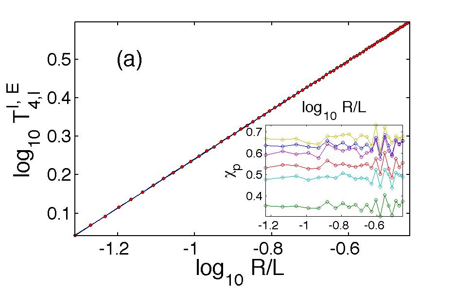
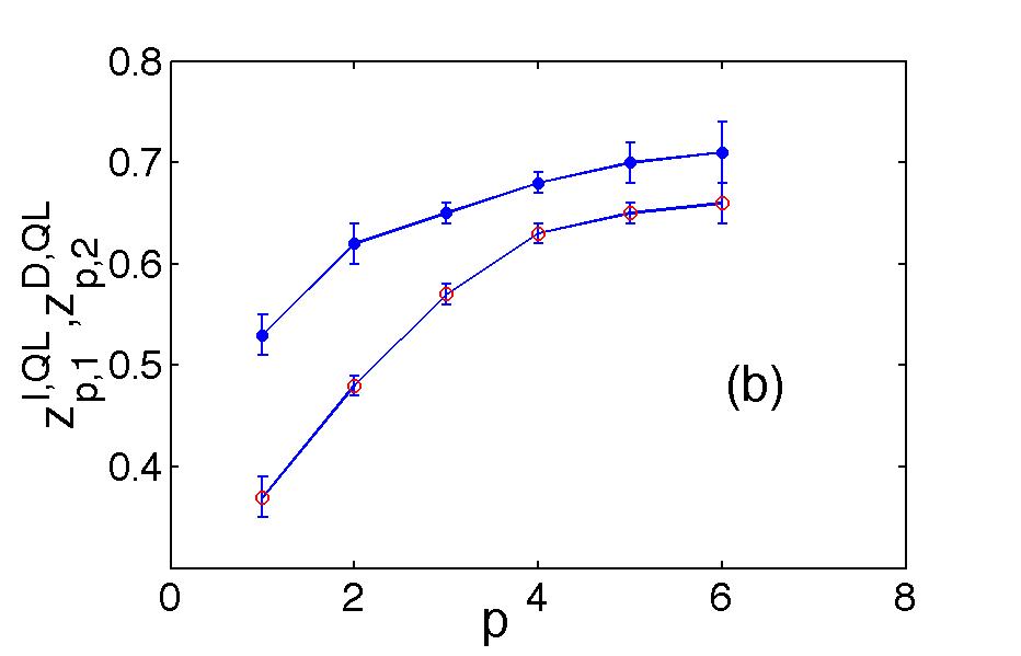
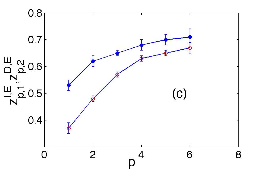
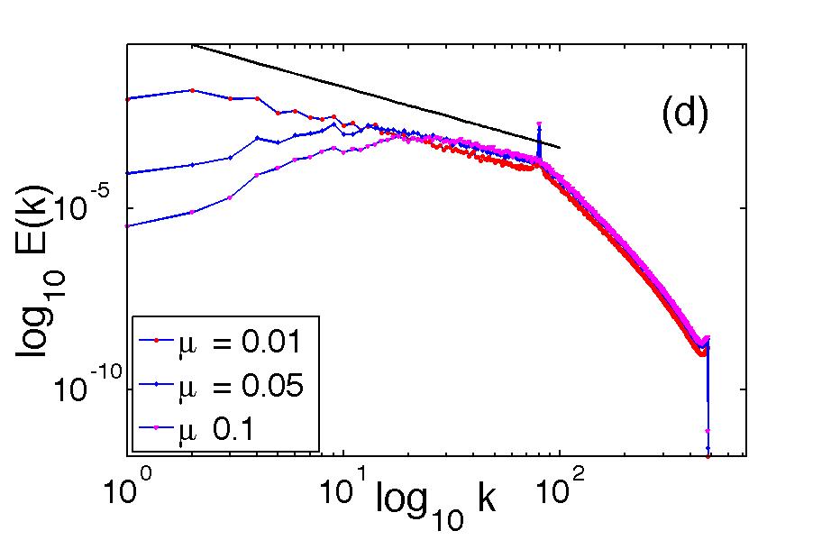
Figure 2: (Color online) (a) Log-log (base 10) plot of the order-2, degree-1, integral time scale $T^{I,{\rm E}}_{4,1}(R^{\prime})$ versus the separation $R^{\prime}$ showing our data points (open red circles) and the best-fit line (full black) in the scaling range; the inset shows the local slopes $\chi_{p}$, obtained as defined in the text, versus the separation, from $p=1$ (bottom) tp $p=6$ (top); (b) plots of the vorticity, dynamic-multiscaling, quasi-Lagrangian exponents $z_{p,1}^{I,{\rm QL}}$ (open red circles) and $z_{p,2}^{D,{\rm QL}}$ (full blue circles) versus $p$ with the error bars given in columns 4 and 6, respectively, in Table I; (c) plots of the vorticity, dynamic-multiscaling, Eulerian exponents $z_{p,1}^{I,{\rm E}}$ (open red circles) and $z_{p,2}^{D,{\rm E}}$ (full blue circles) versus $p$ with the error bars given in columns 4 and 6, respectively, in Table II. (d) log-log (base 10) plot of the energy spectrum $E(k)$ versus the wave-vector magnitude $k$ for $\mu=0.01$ (red filled circles), $\mu=0.05$ (blue filled diamonds), and $\mu=0.1$ (magenta filled triangles); the peak is at the injection scale $k=80$ and the black line indicates the K41, 2D-inverse-cascade slope.

order$(p)$ $\zeta^{{\rm E}}_{p}$ $z^{I,{\rm E}}_{p,1}$[Eq.(6)] $z^{I,{\rm E}}_{p,1}$ $z^{D,{\rm E}}_{p,2}$[Eq.(7)] $z^{D,{\rm E}}_{p,2}$ 1 0.62 $\pm$ 0.009 0.372 $\pm$ 0.009 0.37 $\pm$ 0.02 0.53 $\pm$ 0.02 0.53 $\pm$ 0.02 2 1.13 $\pm$ 0.009 0.51 $\pm$ 0.02 0.48 $\pm$ 0.01 0.60 $\pm$ 0.02 0.62 $\pm$ 0.02 3 1.561 $\pm$ 0.009 0.56 $\pm$ 0.02 0.57 $\pm$ 0.01 0.66 $\pm$ 0.02 0.65 $\pm$ 0.02 4 1.92 $\pm$ 0.01 0.64 $\pm$ 0.02 0.63 $\pm$ 0.01 0.70 $\pm$ 0.03 0.68 $\pm$ 0.02 5 2.24 $\pm$ 0.01 0.68 $\pm$ 0.02 0.65 $\pm$ 0.02 0.71 $\pm$ 0.03 0.70 $\pm$ 0.02 6 2.52 $\pm$ 0.02 0.72 $\pm$ 0.03 0.67 $\pm$ 0.02 0.72 $\pm$ 0.03 0.71 $\pm$ 0.03

Table 2: Order-$p$ (column 1); equal-time, Eulerian exponents $\zeta^{\rm E}_{p}$ (column 2); integral-scale, dynamic-multiscaling exponent $z^{I,{\rm E}}_{p,1}$ (column 3) from the bridge relation and the values of $\zeta^{\rm E}_{p}$ in column 2; $z^{I,{\rm E}}_{p,1}$ from our calculation of time-dependent structure functions (column 4); the derivative-time exponents $z^{D,{\rm E}}_{p,2}$ (column 5) from the bridge relation and the values of $\zeta^{\rm E}_{p}$ in column 2; $z^{D,{\rm E}}_{p,2}$ from our calculation of time-dependent structure function (column 6). The error estimates are obtained as described in the text.