Measurements of branching fractions and asymmetries
and studies of angular distributions for
decays
J. P. Lees
V. Poireau
E. Prencipe
V. Tisserand
Laboratoire d’Annecy-le-Vieux de Physique des Particules (LAPP), Université de Savoie, CNRS/IN2P3, F-74941 Annecy-Le-Vieux, France
J. Garra Tico
E. Grauges
Universitat de Barcelona, Facultat de Fisica, Departament ECM, E-08028 Barcelona, Spain
M. MartinelliabD. A. MilanesaA. PalanoabM. PappagalloabINFN Sezione di Baria; Dipartimento di Fisica, Università di Barib, I-70126 Bari, Italy
G. Eigen
B. Stugu
L. Sun
University of Bergen, Institute of Physics, N-5007 Bergen, Norway
D. N. Brown
L. T. Kerth
Yu. G. Kolomensky
G. Lynch
Lawrence Berkeley National Laboratory and University of California, Berkeley, California 94720, USA
H. Koch
T. Schroeder
Ruhr Universität Bochum, Institut für Experimentalphysik 1, D-44780 Bochum, Germany
D. J. Asgeirsson
C. Hearty
T. S. Mattison
J. A. McKenna
University of British Columbia, Vancouver, British Columbia, Canada V6T 1Z1
A. Khan
Brunel University, Uxbridge, Middlesex UB8 3PH, United Kingdom
V. E. Blinov
A. R. Buzykaev
V. P. Druzhinin
V. B. Golubev
E. A. Kravchenko
A. P. Onuchin
S. I. Serednyakov
Yu. I. Skovpen
E. P. Solodov
K. Yu. Todyshev
A. N. Yushkov
Budker Institute of Nuclear Physics, Novosibirsk 630090, Russia
M. Bondioli
S. Curry
D. Kirkby
A. J. Lankford
M. Mandelkern
D. P. Stoker
University of California at Irvine, Irvine, California 92697, USA
H. Atmacan
J. W. Gary
F. Liu
O. Long
G. M. Vitug
University of California at Riverside, Riverside, California 92521, USA
C. Campagnari
T. M. Hong
D. Kovalskyi
J. D. Richman
C. A. West
University of California at Santa Barbara, Santa Barbara, California 93106, USA
A. M. Eisner
J. Kroseberg
W. S. Lockman
A. J. Martinez
T. Schalk
B. A. Schumm
A. Seiden
University of California at Santa Cruz, Institute for Particle Physics, Santa Cruz, California 95064, USA
C. H. Cheng
D. A. Doll
B. Echenard
K. T. Flood
D. G. Hitlin
P. Ongmongkolkul
F. C. Porter
A. Y. Rakitin
California Institute of Technology, Pasadena, California 91125, USA
R. Andreassen
M. S. Dubrovin
B. T. Meadows
M. D. Sokoloff
University of Cincinnati, Cincinnati, Ohio 45221, USA
P. C. Bloom
W. T. Ford
A. Gaz
M. Nagel
U. Nauenberg
J. G. Smith
S. R. Wagner
University of Colorado, Boulder, Colorado 80309, USA
R. Ayad
Now at Temple University, Philadelphia, Pennsylvania 19122, USA
W. H. Toki
Colorado State University, Fort Collins, Colorado 80523, USA
B. Spaan
Technische Universität Dortmund, Fakultät Physik, D-44221 Dortmund, Germany
M. J. Kobel
K. R. Schubert
R. Schwierz
Technische Universität Dresden, Institut für Kern- und Teilchenphysik, D-01062 Dresden, Germany
D. Bernard
M. Verderi
Laboratoire Leprince-Ringuet, CNRS/IN2P3, Ecole Polytechnique, F-91128 Palaiseau, France
P. J. Clark
S. Playfer
J. E. Watson
University of Edinburgh, Edinburgh EH9 3JZ, United Kingdom
D. BettoniaC. BozziaR. CalabreseabG. CibinettoabE. FioravantiabI. GarziaabE. LuppiabM. MuneratoabM. NegriniabL. PiemonteseaINFN Sezione di Ferraraa; Dipartimento di Fisica, Università di Ferrarab, I-44100 Ferrara, Italy
R. Baldini-Ferroli
A. Calcaterra
R. de Sangro
G. Finocchiaro
M. Nicolaci
S. Pacetti
P. Patteri
I. M. Peruzzi
Also with Università di Perugia, Dipartimento di Fisica, Perugia, Italy
M. Piccolo
M. Rama
A. Zallo
INFN Laboratori Nazionali di Frascati, I-00044 Frascati, Italy
R. ContriabE. GuidoabM. Lo VetereabM. R. MongeabS. PassaggioaC. PatrignaniabE. RobuttiaINFN Sezione di Genovaa; Dipartimento di Fisica, Università di Genovab, I-16146 Genova, Italy
B. Bhuyan
V. Prasad
Indian Institute of Technology Guwahati, Guwahati, Assam, 781 039, India
C. L. Lee
M. Morii
Harvard University, Cambridge, Massachusetts 02138, USA
A. J. Edwards
Harvey Mudd College, Claremont, California 91711
A. Adametz
J. Marks
U. Uwer
Universität Heidelberg, Physikalisches Institut, Philosophenweg 12, D-69120 Heidelberg, Germany
F. U. Bernlochner
M. Ebert
H. M. Lacker
T. Lueck
Humboldt-Universität zu Berlin, Institut für Physik, Newtonstr. 15, D-12489 Berlin, Germany
P. D. Dauncey
M. Tibbetts
Imperial College London, London, SW7 2AZ, United Kingdom
P. K. Behera
U. Mallik
University of Iowa, Iowa City, Iowa 52242, USA
C. Chen
J. Cochran
H. B. Crawley
W. T. Meyer
S. Prell
E. I. Rosenberg
A. E. Rubin
Iowa State University, Ames, Iowa 50011-3160, USA
A. V. Gritsan
Z. J. Guo
Johns Hopkins University, Baltimore, Maryland 21218, USA
N. Arnaud
M. Davier
D. Derkach
G. Grosdidier
F. Le Diberder
A. M. Lutz
B. Malaescu
P. Roudeau
M. H. Schune
A. Stocchi
G. Wormser
Laboratoire de l’Accélérateur Linéaire, IN2P3/CNRS et Université Paris-Sud 11, Centre Scientifique d’Orsay, B. P. 34, F-91898 Orsay Cedex, France
D. J. Lange
D. M. Wright
Lawrence Livermore National Laboratory, Livermore, California 94550, USA
I. Bingham
C. A. Chavez
J. P. Coleman
J. R. Fry
E. Gabathuler
D. E. Hutchcroft
D. J. Payne
C. Touramanis
University of Liverpool, Liverpool L69 7ZE, United Kingdom
A. J. Bevan
F. Di Lodovico
R. Sacco
M. Sigamani
Queen Mary, University of London, London, E1 4NS, United Kingdom
G. Cowan
S. Paramesvaran
University of London, Royal Holloway and Bedford New College, Egham, Surrey TW20 0EX, United Kingdom
D. N. Brown
C. L. Davis
University of Louisville, Louisville, Kentucky 40292, USA
A. G. Denig
M. Fritsch
W. Gradl
A. Hafner
Johannes Gutenberg-Universität Mainz, Institut für Kernphysik, D-55099 Mainz, Germany
K. E. Alwyn
D. Bailey
R. J. Barlow
G. Jackson
G. D. Lafferty
University of Manchester, Manchester M13 9PL, United Kingdom
R. Cenci
B. Hamilton
A. Jawahery
D. A. Roberts
G. Simi
University of Maryland, College Park, Maryland 20742, USA
C. Dallapiccola
E. Salvati
University of Massachusetts, Amherst, Massachusetts 01003, USA
R. Cowan
D. Dujmic
G. Sciolla
Massachusetts Institute of Technology, Laboratory for Nuclear Science, Cambridge, Massachusetts 02139, USA
D. Lindemann
P. M. Patel
S. H. Robertson
M. Schram
McGill University, Montréal, Québec, Canada H3A 2T8
P. BiassoniabA. LazzaroabV. LombardoaF. PalomboabS. StrackaabINFN Sezione di Milanoa; Dipartimento di Fisica, Università di Milanob, I-20133 Milano, Italy
L. Cremaldi
R. Godang
Now at University of South Alabama, Mobile, Alabama 36688, USA
R. Kroeger
P. Sonnek
D. J. Summers
University of Mississippi, University, Mississippi 38677, USA
X. Nguyen
P. Taras
Université de Montréal, Physique des Particules, Montréal, Québec, Canada H3C 3J7
G. De NardoabD. MonorchioabG. OnoratoabC. SciaccaabINFN Sezione di Napolia; Dipartimento di Scienze Fisiche, Università di Napoli Federico IIb, I-80126 Napoli, Italy
G. Raven
H. L. Snoek
NIKHEF, National Institute for Nuclear Physics and High Energy Physics, NL-1009 DB Amsterdam, The Netherlands
C. P. Jessop
K. J. Knoepfel
J. M. LoSecco
W. F. Wang
University of Notre Dame, Notre Dame, Indiana 46556, USA
K. Honscheid
R. Kass
Ohio State University, Columbus, Ohio 43210, USA
J. Brau
R. Frey
N. B. Sinev
D. Strom
E. Torrence
University of Oregon, Eugene, Oregon 97403, USA
E. FeltresiabN. GagliardiabM. MargoniabM. MorandinaM. PosoccoaM. RotondoaF. SimonettoabR. StroiliabINFN Sezione di Padovaa; Dipartimento di Fisica, Università di Padovab, I-35131 Padova, Italy
E. Ben-Haim
M. Bomben
G. R. Bonneaud
H. Briand
G. Calderini
J. Chauveau
O. Hamon
Ph. Leruste
G. Marchiori
J. Ocariz
S. Sitt
Laboratoire de Physique Nucléaire et de Hautes Energies, IN2P3/CNRS, Université Pierre et Marie Curie-Paris6, Université Denis Diderot-Paris7, F-75252 Paris, France
M. BiasiniabE. ManoniabA. RossiabINFN Sezione di Perugiaa; Dipartimento di Fisica, Università di Perugiab, I-06100 Perugia, Italy
C. AngeliniabG. BatignaniabS. BettariniabM. CarpinelliabAlso with Università di Sassari, Sassari, Italy
G. CasarosaabA. CervelliabF. FortiabM. A. GiorgiabA. LusianiacN. NeriabB. OberhofabE. PaoloniabA. PerezaG. RizzoabJ. J. WalshaINFN Sezione di Pisaa; Dipartimento di Fisica, Università di Pisab; Scuola Normale Superiore di Pisac, I-56127 Pisa, Italy
D. Lopes Pegna
C. Lu
J. Olsen
A. J. S. Smith
A. V. Telnov
Princeton University, Princeton, New Jersey 08544, USA
F. AnulliaG. CavotoaR. FacciniabF. FerrarottoaF. FerroniabM. GasperoabL. Li GioiaM. A. MazzoniaG. PireddaaINFN Sezione di Romaa; Dipartimento di Fisica, Università di Roma La Sapienzab, I-00185 Roma, Italy
C. Bünger
T. Hartmann
T. Leddig
H. Schröder
R. Waldi
Universität Rostock, D-18051 Rostock, Germany
T. Adye
E. O. Olaiya
F. F. Wilson
Rutherford Appleton Laboratory, Chilton, Didcot, Oxon, OX11 0QX, United Kingdom
S. Emery
G. Hamel de Monchenault
G. Vasseur
Ch. Yèche
CEA, Irfu, SPP, Centre de Saclay, F-91191 Gif-sur-Yvette, France
D. Aston
D. J. Bard
R. Bartoldus
J. F. Benitez
C. Cartaro
M. R. Convery
J. Dorfan
G. P. Dubois-Felsmann
W. Dunwoodie
R. C. Field
M. Franco Sevilla
B. G. Fulsom
A. M. Gabareen
M. T. Graham
P. Grenier
C. Hast
W. R. Innes
M. H. Kelsey
H. Kim
P. Kim
M. L. Kocian
D. W. G. S. Leith
P. Lewis
S. Li
B. Lindquist
S. Luitz
V. Luth
H. L. Lynch
D. B. MacFarlane
D. R. Muller
H. Neal
S. Nelson
I. Ofte
M. Perl
T. Pulliam
B. N. Ratcliff
A. Roodman
A. A. Salnikov
V. Santoro
R. H. Schindler
A. Snyder
D. Su
M. K. Sullivan
J. Va’vra
A. P. Wagner
M. Weaver
W. J. Wisniewski
M. Wittgen
D. H. Wright
H. W. Wulsin
A. K. Yarritu
C. C. Young
V. Ziegler
SLAC National Accelerator Laboratory, Stanford, California 94309 USA
W. Park
M. V. Purohit
R. M. White
J. R. Wilson
University of South Carolina, Columbia, South Carolina 29208, USA
A. Randle-Conde
S. J. Sekula
Southern Methodist University, Dallas, Texas 75275, USA
M. Bellis
P. R. Burchat
T. S. Miyashita
Stanford University, Stanford, California 94305-4060, USA
M. S. Alam
J. A. Ernst
State University of New York, Albany, New York 12222, USA
R. Gorodeisky
N. Guttman
D. R. Peimer
A. Soffer
Tel Aviv University, School of Physics and Astronomy, Tel Aviv, 69978, Israel
P. Lund
S. M. Spanier
University of Tennessee, Knoxville, Tennessee 37996, USA
R. Eckmann
J. L. Ritchie
A. M. Ruland
C. J. Schilling
R. F. Schwitters
B. C. Wray
University of Texas at Austin, Austin, Texas 78712, USA
J. M. Izen
X. C. Lou
University of Texas at Dallas, Richardson, Texas 75083, USA
F. BianchiabD. GambaabINFN Sezione di Torinoa; Dipartimento di Fisica Sperimentale, Università di Torinob, I-10125 Torino, Italy
L. LanceriabL. VitaleabINFN Sezione di Triestea; Dipartimento di Fisica, Università di Triesteb, I-34127 Trieste, Italy
N. Lopez-March
F. Martinez-Vidal
A. Oyanguren
IFIC, Universitat de Valencia-CSIC, E-46071 Valencia, Spain
H. Ahmed
J. Albert
Sw. Banerjee
H. H. F. Choi
G. J. King
R. Kowalewski
M. J. Lewczuk
C. Lindsay
I. M. Nugent
J. M. Roney
R. J. Sobie
University of Victoria, Victoria, British Columbia, Canada V8W 3P6
T. J. Gershon
P. F. Harrison
T. E. Latham
E. M. T. Puccio
Department of Physics, University of Warwick, Coventry CV4 7AL, United Kingdom
H. R. Band
S. Dasu
Y. Pan
R. Prepost
C. O. Vuosalo
S. L. Wu
University of Wisconsin, Madison, Wisconsin 53706, USA
Abstract
We present branching fraction and asymmetry measurements
as well as angular studies of
decays
using events collected by the BABAR experiment.
The branching fractions are measured in the
invariant mass range below the resonance ( GeV).
We find
and
,
where the first uncertaintiy is statistical and the second systematic.
The measured direct asymmetries for the decays are
below the threshold ( GeV)
and
in the resonance region
( in [2.94,3.02] GeV).
Angular distributions are consistent with in the resonance region
and favor below the resonance.
pacs:
13.25.Hw, 14.40.Nd
††preprint: BABAR-PUB-07/x††preprint: SLAC-PUB-x
The violation of symmetry is a well-known requirement for the matter-antimatter
imbalance of the universe sakarov .
The BABARbabarnim and Belle bellenim experiments at the high-luminosity factories,
PEP-II pepii and KEKB kekb , have made numerous
asymmetry measurements using datasets
two orders of magnitude larger than their predecessors.
All of these measurements are consistent with a single source of violation –
the complex phase within the CKM quark mixing matrix of the Standard Model km .
However, with the small amount of violation from the CKM matrix, it
is difficult to explain the matter-antimatter asymmetry of the
universe matter-antimatter-asym .
This motivates searches for new sources of violation.
A method to search for new sources of -violating phases is to measure
asymmetries in hadron decays that are forbidden at the tree level grossman .
Since the leading decay amplitude is a one-loop process, contributions
within the loop from virtual non-Standard-Model particles cannot be excluded.
The quark interactions with the non-Standard-Model particles can introduce
new violating phases in the decay amplitude, which can lead to
observable non-zero asymmetries.
Decays of mesons with a transition have been extensively
studied for this reason.
The three body decay is a one-loop “penguin”
transition.
This final state can also occur through the tree-level decay
,
followed by
,
where
the decay is a transition.
If the invariant mass in the
three-body decay is close to the
resonance, the tree and penguin amplitudes may interfere.
Within the Standard Model, the relative weak phase between these
amplitudes is , so
no violation is expected from the interference.
However, new physics contributions to the penguin loop in the
decay could introduce a non-zero relative
violating phase, which may then produce a significant
direct asymmetry hazumi .
Measurement of a significant, non-zero direct asymmetry
would be an unambiguous
sign of new physics.
A previous measurement of the direct asymmetry belle-ppk
was consistent with zero, but was also limited by a large statistical
uncertainty.
The and branching
fractions have been previously measured belle-ppk old-babar-ppk
to be a few times .
Theoretical predictions of the branching fractions are of the
same order fajfer chen .
I Dataset and Detector description
We present measurements of the and branching fractions chargeconj and direct asymmetry
as well as studies of angular distributions
performed using
pairs collected by the BABAR experiment
at the SLAC National Accelerator Laboratory.
The direct asymmetry is measured both below and within the
resonance region of the invariant mass
with these regions defined as GeV and within
[2.94, 3.02] GeV, respectively c=1 .
The branching fractions are measured in the region below the
resonance ( GeV).
The BABAR detector is described in detail elsewhere babarnim .
What follows is a brief overview of the main features of the detector.
The detector has a roughly cylindrical geometry, with the axis along
the beam direction.
The trajectories, momenta, and production vertices of charged particles
are reconstructed from position measurements made by a silicon
vertex tracker (SVT) and a 40-layer drift chamber (DCH).
The SVT consists of 5 layers of double-sided silicon strip detectors
which provide precision position measurements close to the beam interaction region.
Both the SVT and DCH measure the specific energy loss () along
the charged particle trajectory, which is used to infer the particle
mass from the velocity dependence of the energy loss and the momentum
measurement.
The tracking system is inside a uniform 1.5 T magnetic field provided
by a superconducting solenoid.
Outside the tracking system, an array of quartz bars coupled with an array of phototubes
(DIRC) detects the Cherenkov light produced when a charged particle travels
through the quartz bars.
The measured Cherenkov angle is used to infer the particle mass from the velocity
dependence of the Cherenkov angle and the measured momentum.
The energies of photons and electrons are determined from the measured light produced
in electromagnetic showers inside a CsI crystal calorimeter (EMC).
Gaps in the iron of the magnet flux return are instrumented with resistive plate chambers
and limited streamer tubes, which are used to identify muons and neutral hadrons (IFR).
We use Monte Carlo (MC) samples to determine the signal selection efficiency.
The MC events are generated with EvtGen evtgen and simulated using
Geant4geant4 .
II Event selection
We select
events containing multiple hadrons by requiring at least three charged tracks
in the event and
the ratio of the second to zeroth Fox-Wolframfox-wolfram moments to be less than 0.98.
Charged kaon candidates are required to pass a selection based on a likelihood ratio
which uses the SVT and DCH and the DIRC Cherenkov angle measurements
as inputs to the likelihood.
The ratio is defined as , where
and are , , or .
The minimum kaon selection criterion is or .
This selection has an efficiency greater than 98% for kaons
and a pion efficiency of less than 15%
below a lab momentum of 2.5 GeV.
Candidate decays are constructed from oppositely-charged kaon
candidates with an invariant mass in the range of 0.987 to 1.2 GeV.
At least one of the kaons in each candidate must also satisfy the
more stringent criteria of and ,
which has an efficiency greater than 90% for kaons and a pion efficiency of less than 3%
below a lab momentum of 2.5 GeV.
Candidate decays are constructed from oppositely-charged
pion candidates with an invariant mass in the range of 0.486 to 0.510 GeV.
The pion tracks are fit to a common vertex.
The probability of the vertex fit must be greater than 0.001.
The typical experimental resolution on the measured flight length in the
plane transverse to the beam is around 0.2 mm or less.
We require the transverse flight length to be at least 2 mm.
Candidate decays are constructed from
pairs of candidates that do not share any daughters
and either a or a candidate.
The and candidates are constrained to a common vertex.
We reject
combinatoric background by requiring the candidate to have
kinematics consistent with using two standard
variables: and .
The energy-substituted mass is defined as ,
where and are the beam energy () and the reconstructed
momentum, both in the center-of-mass (CM) reference frame.
The energy difference is defined as ,
where is the reconstructed energy in the CM frame.
We require and to be within [5.20, 5.29] GeV and
[] GeV, respectively.
The experimental resolution is about 2.7 MeV for
and 15 MeV for .
The interval includes a large “sideband” region
below the area where the signal is concentrated near the mass.
The interval also is wide enough to include sideband regions
where the signal probability is very low.
Including events in the sideband regions
enables us to determine the probability density functions (PDFs) of the
combinatoric background directly in the maximum likelihood (ML)
fits of the data.
About 7% of events in signal Monte Carlo samples have more than
one candidate.
If there are multiple candidates in a single event,
we select the candidate with the smallest mass defined as
, where
the sum is over the two candidates,
() is the reconstructed (nominal) mass,
and is the RMS of the reconstructed distribution
for properly reconstructed candidates.
If there are more than one candidates that use the same two
candidates, we choose the candidate with the highest
quality identification for the from the decay.
If the quality level of the identification is the same for
these candidates, we choose the candidate with the
highest vertex probability.
For events with multiple , the sum for
includes the , and we choose
the with the smallest .
For both the and decay modes,
the probability that the the algorithms described
above choose the correct candidate is about 87%.
The reconstruction and selection efficiencies for events with
GeV are determined from Monte Carlo samples to be
28.0% and 22.5% for the and modes, respectively.
We use control samples of decays where ,
, and to determine corrections to the
signal probability density function parameters
determined from Monte Carlo samples in the maximum likelihood fits described below.
II.1 Continuum Background
The events that pass the selection above with at least one candidate are
primarily background events from the continuum ( with
).
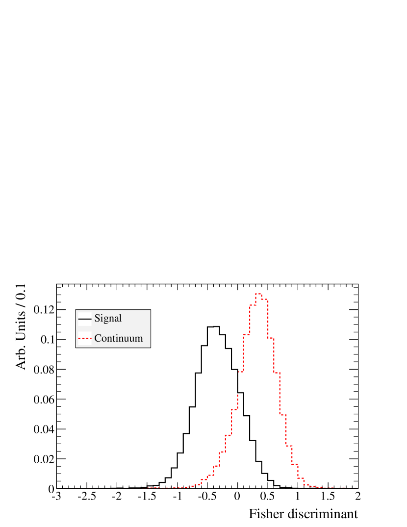
We reduce this background by using a Fisher discriminant (),
which is the linear combination of seven variables and is optimized for maximum
separation power of signal and the continuum background.
The seven variables are listed below.
These variables are commonly used by the BABAR experiment in analyses of
charmless decays, where the primary background is from continuum
events.
They take advantage of aspects of the production distributions and event
topologies of versus continuum production events.
•
: the absolute value of the
reconstructed proper time difference between the two decays divided by
its uncertainty dtandft .
•
: the absolute value of the standard BABAR flavor
tagging neural network output dtandft .
•
: the absolute value of the cosine
of the angle between the candidate thrust axis and the thrust axis of the
rest of the event computed in the CM frame.
The thrust axis is the direction that maximizes the scalar sum of the projection
of the track momenta on that direction.
•
: the absolute value of the cosine
between the thrust axis of the candidate and the beam axis in the
CM frame. Signal events have a uniform distribution in this variable, while
continuum background follows a distribution, where
is the angle between the thrust direction and the beam axis.
•
: the absolute value of the cosine
of the angle between the direction and the beam axis in
the CM frame.
The angular distribution of the signal follows a distribution,
while the continuum background is uniformly distributed.
•
and : The zeroth and second angular moments of
the momentum flow of the rest of the event about the thrust axis, defined as
, where the angle
is the angle between track and the thrust axis
and the sum excludes the daughters of the candidate.
The calculations are done in the CM frame.
Distributions of for signal and continuum MC samples
are shown in Fig. 1.
The Fisher discriminant is used as one of several variables
in the maximum likelihood fits described below.
Figure 1: Distributions of the Fisher discriminant
for signal (solid black) and
continuum (dashed red) Monte
Carlo simulation.
II.2 Peaking Backgrounds
The ultimate detected state of our signal decay is five kaons.
In addition to the resonance, there may be contributions to
each pair either from other intermediate resonances,
such as the , or from non-resonant contributions.
We use the mass sidebands for each candidate to determine
the amount of mesons that decay to the detected five-kaon state
(which we denote )
that are not coming from .
The specific decays that we consider as backgrounds are
,
,
, and
.
The branching fractions for these decays are currently unknown.
We call these decays “peaking backgrounds” because properly reconstructed
candidates are indistinguishable from our signal in
the , , and variables.
We perform unbinned extended maximum likelihood fits to determine the signal
and combinatoric background yields and, in some cases, the charge asymmetry.
All of the fits use the product of one-dimensional
PDFs of , , and in the likelihood.
For the branching fraction measurements, we also include
PDFs for the invariant mass of each candidate (
and ).
As a first step, we divide the vs. plane phi-assignment
in the range of 0.987 to 1.200 GeV
into five mutually exclusive zones.
We fit for the yield in each zone using only
, , and in the likelihood.
The zones are based on various combinations of the signal and sideband regions,
which are defined as: Low-SB [0.987,1.000] GeV, phi-signal [1.00,1.04] GeV,
and High-SB [1.04,1.20] GeV.
Each of the five zones is chosen so that either the signal or
one of the four peaking backgrounds is concentrated in the region.
We compute the number of peaking background events within the
range used for the branching fraction fit by using the results of the
five zone fits as described below.
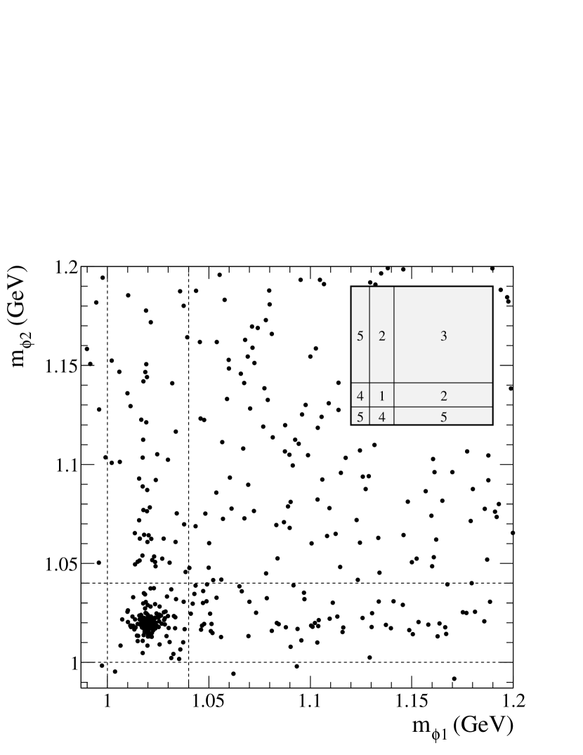
Figure 2 shows the distribution of events in
the vs. plane for the selected
candidates in the data.
To enhance the signal for the figure,
we have required GeV,
GeV, and
.
The inset of the figure shows the definition of the five zones.
A concentration of events in the phi-signal region for both
candidates (zone 1) is clearly evident.
The region defined as phi-signal combined with High-SB for either
candidate (zone 2) contains the largest fraction of the
mode, although the signal also
populates this region due to cases where one is mis-reconstructed.
The zone where the invariant mass of both candidates is in
the High-SB region (zone 3) contains the largest concentration
of the non-resonant mode.
Zones 4 and 5 contain a large fraction of the and
modes, respectively, and very small fractions of
the other three modes.
Figure 2: Data distribution of events in the vs. plane
for events with GeV.
To enhance the signal for the figure, we have required
GeV, GeV,
and
.
The efficiency of these additional requirements, relative
to the nominal selection, is about 70% for the signal.
The inset shows the definition of the five zones.
Monte Carlo samples for the five decay modes (signal plus four
peaking background modes) are used to determine the fraction of
events in each zone () for each decay mode (), which we
denote with the matrix .
The total yield () is determined for each
zone using five separate maximum likelihood fits of the data.
The yield for each decay mode () and the amount of each
mode in zone () can be determined from
(1)
Zone 1 corresponds to the range used in the branching fraction
maximum likelihood fit.
II.3 Maximum Likelihood Fits
The extended maximum likelihood fits in the five zones determine the
signal and combinatoric background yields in each zone.
The signal is split into properly reconstructed and
misreconstructed (“self-crossfeed”) components, with the
self-crossfeed fraction fixed.
The self-crossfeed component is defined as events where
a true decay is present in the event, but one
or more tracks used in the reconstructed are either
from the other in the event or not real.
In zone 1,
the self-crossfeed fraction for decays is
around 7%.
The properly reconstructed signal component is described by
the following PDFs:
a Crystal Ball function CB-function for ,
the sum of three Gaussians for ,
and the sum of a bifurcated Gaussian and a Gaussian for .
The Crystal Ball function is a Gaussian modified to have an extended
power-law tail on the low side.
The signal PDF parameters are determined from MC
samples with corrections to the and core
mean and width parameters from the control samples.
The mean corrections are MeV and MeV
for and , respectively.
The width scale factors are and
for and , respectively.
The combinatoric background is described by the following PDFs:
an empirical threshold function Argus-function for ,
a first-order polynomial for ,
and the sum of two Gaussians for .
Most of the combinatoric background PDF shape parameters are determined
in the fits.
The results of the five zone fits for the and modes are
given in Tables 5 and 6, respectively,
in the appendix.
The signal is observed in both the and samples.
The decay has not been observed previously.
The yield in zone 2 for the mode is significant, but about half of
this is due to misreconstructed signal.
The computed and yields
are positive, but the significance is less than two standard deviations.
There is no evidence of either or .
The branching fraction maximum likelihood fits use the range
that corresponds to zone 1.
We fix the yield of each of the four peaking background modes to the
zone 1 value in Table 5 or 6
for the branching fraction fit described below.
III Branching Fraction Analysis
The maximum likelihood fit used to measure the yield
below the resonance for the branching fraction
measurement restricts
the event selection with GeV and
within [1.00,1.04] GeV, which corresponds to zone 1 in
the peaking background discussion above.
The fit components are signal,
combinatoric background,
and the four peaking backgrounds.
In addition to , , and , PDFs for
and are included in the likelihood function.
For each fit component, each candidate has a PDF that is the sum
of a properly reconstructed decay,
given by a relativistic Breit-Wigner function,
and a misreconstructed , described by a first-order polynomial.
The and PDFs are combined in a way that
is symmetric under exchange and
takes into account the fractions of events where both candidates are
properly reconstructed, one is misreconstructed, and
both candidates are misreconstructed.
In addition to the signal and combinatoric background yields,
the charge asymmetry for the signal and combinatoric background
components and most of the combinatoric background PDF parameters
are determined in the fit.
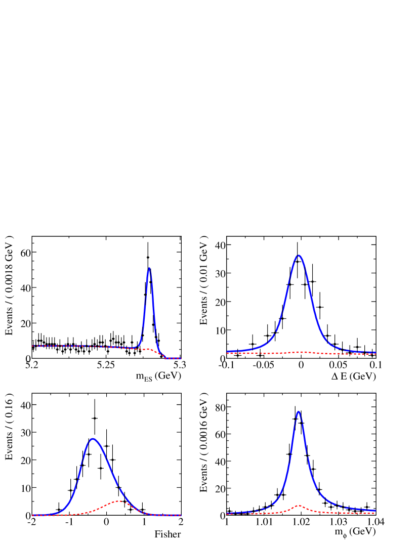
The results of the and fits are shown in Figs. 3
and 4, respectively.
To reduce the combinatoric background in each distribution
shown in the figures, a requirement is made on a likelihood
ratio, which is based on all the fit variables except the one plotted.
Figure 3: Results of fitting the sample for
GeV.
The dashed red curve is the sum of the combinatoric
and peaking background components.
The solid blue curve is for all components.
A requirement on a likelihood ratio based on all fit variables
except the one plotted is made to reject most of
the background.
The likelihood ratio requirements are about 84% efficient for
the signal.
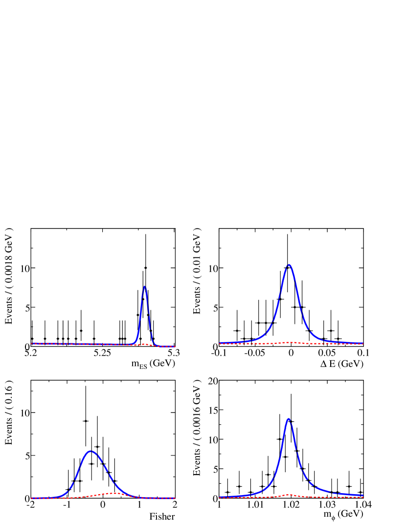
Figure 4: Results of fitting the sample for
GeV.
The dashed red curve is the sum of the combinatoric
and peaking background components.
The solid blue curve is for all components.
A requirement on a likelihood ratio based on all fit variables
except the one plotted is made to reject most of
the background.
The likelihood ratio requirements are about 84% efficient for
the signal.
The fitted charge asymmetry for the background component
is .
The charge asymmetry for the signal component is .
The fitted yields of and signal candidates
with GeV
are events and events, respectively,
where the uncertainties are statistical only.
III.1 Systematic Uncertainties
Table 1 summarizes the systematic uncertainties on the
branching fractions in the GeV region.
The systematics are divided into additive uncertainties that affect the
yield measurement
and multiplicative uncertainties
in the branching fraction calculation.
The uncertainties from the corrections applied to the PDF parameters
such as the and core mean and width
for the signal component,
which are derived from data control samples, are listed under “ML Fit Yield”.
The signal Fisher and core Gaussian mean and width parameters
are not corrected in the fit, because data control sample measurements
are consistent with the Monte Carlo.
However, we did vary the signal Fisher and core Gaussian mean and
width parameters by the statistical uncertainty of the data control sample
measurements. These variations are also included under “ML Fit Yield”.
The fit bias systematic is taken to be half of the bias correction added in
quadrature with the statistical uncertainty on the bias.
We vary the fixed peaking background yields by their statistical uncertainties
(see Tables 5 and 6)
and by varying the fractions .
The fixed self-crossfeed fraction for the signal component was varied by %.
Adding the individual uncertainties in quadrature, the total additive systematic
uncertainties on the and signal yields are 6.2 and 1.8 events, respectively.
The uncertainty on the track reconstruction efficiency is % per track,
which is taken to be fully correlated for the charged kaons.
The reconstruction efficiency has an uncertainty of 1.5%.
The and branching fractions are taken
from the PDG pdg and are varied by their one standard deviation uncertainties.
The systematic uncertainty on the identification criteria was estimated by
comparing the ratio of the yield with the nominal selection to the yield
requiring all to pass the tighter selection in the data and the MC samples.
This gives an uncertainty of 3% for the mode and 2% for the mode.
Adding the individual uncertainties in quadrature, the overall multiplicative
systematic uncertainties are 3.6% for the mode and 3.2% for the mode.
Table 1: Summary of the systematic and statistical uncertainties
for the branching fraction measurements.
Quantity
Fit Stat. Uncertainty (events)
15.1
7.0
Additive Uncertainties (events)
ML Fit Yield
3.3
1.0
ML Fit Bias
1.6
0.2
Peaking BG, region fits
3.5
1.2
Peaking BG, values
3.0
0.8
Self-Crossfeed Fraction
1.8
0.4
Total Additive Syst. (events)
6.2
1.8
Multiplicative Uncertainties (%)
Tracking Efficiency
1.2
1.0
Reconstruction Efficiency
-
1.5
Number
1.1
1.1
()
1.2
1.2
()
-
0.1
MC Statistics
0.1
0.1
Cut Efficiency
0.2
0.3
Identification
3.0
2.0
Total Multiplicative Syst. (%)
3.6
3.2
Total Systematic [] ()
0.3
0.3
Statistical [] ()
0.5
0.8
The signal charge asymmetry has been corrected for a bias due to differences in the
and efficiencies by adding to the asymmetry.
The overall 2% systematic uncertainty takes into account uncertainties
on the charge dependence of the tracking efficiency, material interaction cross
section for kaons, and particle identification.
III.2 Branching Fraction Results
Table 2 summarizes the branching
fraction results for GeV.
We find
where the first uncertainty is statistical and the second systematic.
These results are consistent with and supersede the previous measurements old-babar-ppk
by the BABAR Collaboration.
The Belle collaboration measurements belle-ppk are lower, though
they are statistically compatible.
Our branching fraction measurements are higher than the theoretical
predictions of fajfer and chen .
Table 2: Branching fraction and charge asymmetry results for in the
region GeV.
The statistical significance is given by ,
where is the maximum likelihood and
is the likelihood for the hypothesis of no signal.
The significance does not include systematic uncertainties.
Events to fit
1535
293
Fit signal yield
178 15
40 7
ML-fit bias (events)
3.0 0.5
0.0 0.2
MC efficiency (%)
28.0
22.5
(%)
24.2
8.4
Stat. significance
24
11
()
5.6 0.5 0.3
4.5 0.8 0.3
Signal
-
Comb. Bkg.
0.02 0.03
-
IV CP asymmetry in resonance region
As was mentioned in the introduction, a significant non-zero direct asymmetry
in the resonance region of would be a clear
sign of physics beyond the Standard Model.
For this measurement, we use the simpler likelihood, based on
, , and .
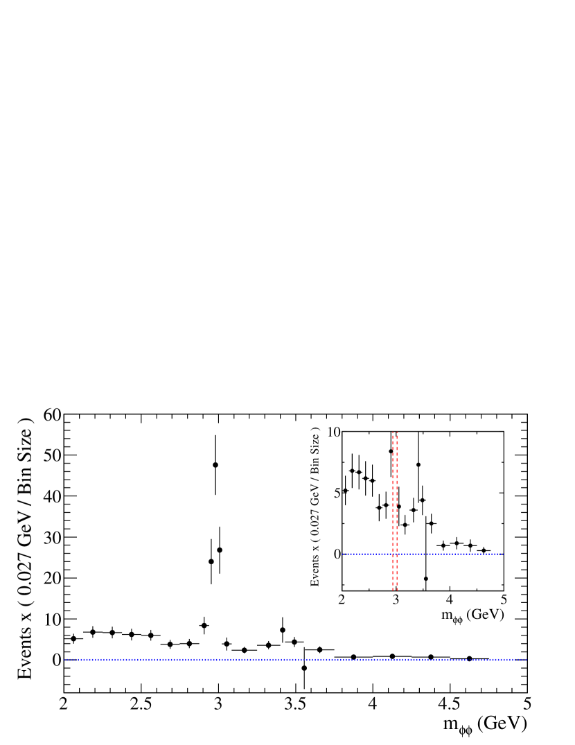
Figure 5 shows the fitted yield as a function
of .
The resonance is clearly visible.
Narrow bins around the and resonances do not show a
significant excess above the broad non-resonant component.
Figure 5: Fitted yield as a function
of .
Each point shows the results of a maximum likelihood
fit of the events in that bin.
The inset is the same data with an expanded vertical
range to show the shape of the non-resonant component
more clearly.
The yield has been divided by the bin width
and scaled by 0.027 GeV, which is the bin width
of the three bins in the
resonance region ([2.94,3.02] GeV
and dashed vertical lines in the inset).
The two narrow bins above the are
centered on the (bin range [3.400,3.430] GeV)
and the (bin range [3.552,3.560] GeV).
The results of fitting the events in the range
of [2.94,3.02] GeV are given in Table 3.
For the asymmetry, we find
where the first uncertainty is statistical and the second uncertainty is
systematic.
The value above includes the same 1% bias correction
and has the same 2% overall systematic uncertainty as
the signal charge asymmetry below the resonance
as described above.
The fit yields signal candidates.
Using
and from the PDG pdg ,
a ; reconstruction efficiency of 29%
in the resonance region,
and an efficiency of 78% for the window of
[2.94,3.02] GeV for the resonance, we would
expect signal events, ignoring the non-resonant
contribution and any interference between the resonant and non-resonant
amplitudes.
We do not use our event yield to measure
due to
the potentially large interference effects between the resonant and non-resonant
amplitudes which we can not easily quantify.
The may integrate to zero, even if there is a contributing
non-Standard-Model amplitude with a non-zero violating phase.
However, in this case the phase variation of the resonance amplitude
could give non-zero values with opposite signs
above and below the peak of the resonance.
We have performed the measurement in two ranges, splitting the
region into two regions (above and below the peak of the resonance).
The results are
both of which are consistent with zero, as expected in the Standard Model.
Table 3: Fit results for within
resonance region ( within [2.94,3.02] GeV).
The signal charge asymmetry has been
corrected by adding to the fitted asymmetry.
ML fit quantity/Analysis
Events to fit
181
Fit signal yield
100 10
MC efficiency (%)
29.2
Corr. Signal
Comb. Bkg.
V Angular Studies
We use the angular variables that describe the decay
to investigate the spin components of the system
below and within the resonance.
The angles are defined as follows.
•
, : The angle is
the angle between the momentum of the coming from the
decay of
in the rest frame with respect to the boost direction from
the rest frame to the rest frame.
•
: The angle is the dihedral angle between
the and decay planes in the rest frame.
•
: The angle
is the angle between one of the mesons in rest
frame with respect to the boost direction from the rest frame
to the rest frame.
We project the component by making a histogram
of weighting each event by
(2)
where is a second-degree Legendre polynomial and is
a spherical harmonic with and .
In each bin, the component yield is projected out,
while the combinatoric background averages to zero.
To do this, we select events in a signal region defined by:
GeV, MeV, within [1.01,1.03] GeV,
and
.
The efficiency of these requirements, relative to the selection used
in the asymmetry measurement, is about 78% for signal events and 2.9%
for combinatoric background.
The combinatoric background that remains after this selection is shown using
data events in the sideband region ( GeV and MeV)
scaled by 0.065, which is the signal-to-sideband ratio for the combinatoric
background.
The results are shown in Fig. 6.
The weighted yield in the region is consistent with all of the
events having .
Just below the region, the weighted yield is consistent with zero.
The excess in the bins near 2.2 GeV may be due
to the seen in events at
Mark III markIII and BES BES .
Figure 7 shows background-subtracted distributions
of , , and for the
nominal event selection.
The background subtraction is done with the technique described
in reference splots .
Since there is no meaningful distinction between and ,
we combine the and distributions into
one plot of .
The reconstruction and selection efficiency, determined
from MC samples, is uniform in and
, but not in , so the
distribution is efficiency corrected.
For each distribution, we performed a simple least- fit
to the distributions expected
for both and for the system.
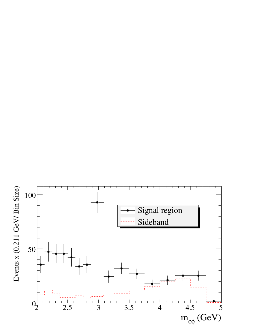
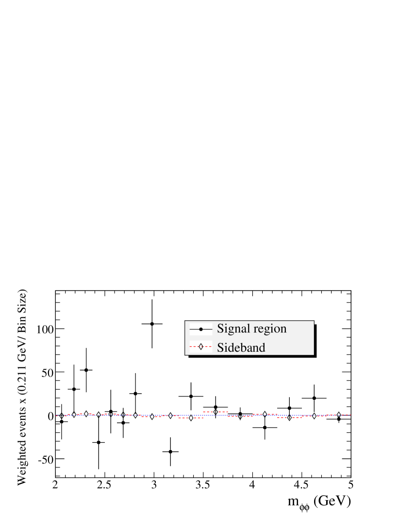
Figure 6:
Histograms (top) and weighted distributions (bottom) of for the
signal region (solid points) and data sideband selection (dashed with
open diamonds) defined in the text.
The sideband distributions have been normalized to the expected level
of combinatoric background remaining after the signal region selection.
Events in the bottom distribution were weighted by
which projects out the component.
The yield has been divided by the bin width
and scaled by 0.211 GeV, which is the
width of the bin covering the
resonance ([2.875,3.086] GeV).
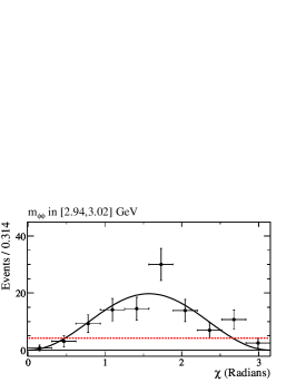
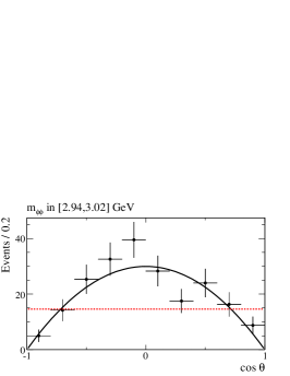
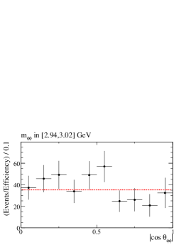
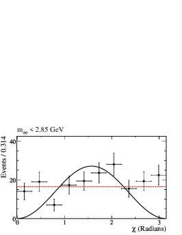
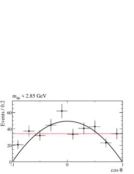
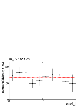
Figure 7:
Background subtracted angular distributions in the resonance
region ( in [2.94,3.02] GeV for the top row) and below
the resonance ( GeV for the bottom row).
The reconstruction and selection efficiency is uniform in
(left) and (center), but dependent on
(right), so the right column has
been efficiency corrected.
The red dashed line shows a least- fit of the points to a uniform
distribution while the solid black curve shows a fit to the expectation
for a state decaying to .
Table 4: Quality of the angular fits shown in Fig. 7.
The first column is the interval for the events in the
fit. The last column is the -value of the goodness-of-fit
test for the hypothesis indicated in the third column.
(GeV)
Variable
PDF
prob.
uniform
uniform
uniform
uniform
uniform
uniform
For a state, we expect to have a
distribution, while should be uniform for .
The signal events in the resonance region are consistent with a
distribution while the signal below the resonance
is not.
For a state, the distributions of are
expected to have distributions, while
a state is expected to have uniform distributions.
The events in the resonance region are consistent with
a distribution,
while the events below the resonance show a deviation from
a shape.
Finally, a spin-zero state should have a uniform
distribution.
The efficiency-corrected distributions shown in
Fig. 7, both within and below the
resonance region, are consistent with a uniform
distribution.
VI Summary and Conclusions
We have measured the branching fractions and charge asymmetries of
decays below the resonance in the
invariant mass ( GeV).
We observe both and ,
each with a significance of greater than five standard deviations.
The decay has not been observed previously.
Our branching fraction measurements are higher than the theoretical
predictions of fajfer and chen .
We have measured the charge asymmetry for in the
resonance region, where a significant non-zero value would
be an unambiguous indication of new physics.
Our measurement is consistent with zero, which is the expectation of
the Standard Model.
Finally, we have studied the angular distributions of
decays below and within the resonance.
We conclude from these studies that the non-resonant
events below the resonance are, on average, more consistent with
than , while
the distributions within the resonance region are all consistent
with .
We are grateful for the
extraordinary contributions of our PEP-II colleagues in
achieving the excellent luminosity and machine conditions
that have made this work possible.
The success of this project also relies critically on the
expertise and dedication of the computing organizations that
support BABAR.
The collaborating institutions wish to thank
SLAC for its support and the kind hospitality extended to them.
This work is supported by the
US Department of Energy
and National Science Foundation, the
Natural Sciences and Engineering Research Council (Canada),
the Commissariat à l’Energie Atomique and
Institut National de Physique Nucléaire et de Physique des Particules
(France), the
Bundesministerium für Bildung und Forschung and
Deutsche Forschungsgemeinschaft
(Germany), the
Istituto Nazionale di Fisica Nucleare (Italy),
the Foundation for Fundamental Research on Matter (The Netherlands),
the Research Council of Norway, the
Ministry of Education and Science of the Russian Federation,
Ministerio de Ciencia e Innovación (Spain), and the
Science and Technology Facilities Council (United Kingdom).
Individuals have received support from
the Marie-Curie IEF program (European Union), the A. P. Sloan Foundation (USA)
and the Binational Science Foundation (USA-Israel).
Appendix A Peaking background zone fit results
The results of the fits of the yield in
the five zones in the vs
plane (shown in Fig. 2)
and the derived yields for each of the five decay
modes are given in Tables 5 and 6
below.
Table 5:
yield fit results for the five zones ( yield column)
and yields derived from the fraction matrix .
The last row is computed from the inverted fraction matrix
and the yield column.
The remaining yield matrix was computed from the last row and the
fraction matrix .
The uncertainties are from propagating the statistical errors from
the fitted region yields ( yield column) without including any
uncertainties on the fraction matrix.
Zone
yield
1
2
36
39
9
-1.4
2
3
3.8
18
26
-0.2
2.2
4
1.3
0.9
0.2
-1.7
0.3
5
0.2
0.8
1.3
-0.2
1.3
Table 6:
yield fit results for the five zones ( yield column)
and yields derived from the fraction matrix .
The last row is computed from the inverted fraction matrix
and the yield column.
The remaining yield matrix was computed from the last row and the
fraction matrix .
The uncertainties are from propagating the statistical errors from
the fitted region yields ( yield column) without including any
uncertainties on the fraction matrix.
Zone
yield
1
2
8
7
0.9
-0.4
-0.4
3
1
3
2.5
-0.1
-0.4
4
0.3
0.2
0
-0.5
0
5
0
0.1
0.1
0
-0.2
References
(1) A.D. Sakharov, JETP Lett. 5, 24 (1967).
(2) B. Aubert et al. [The BABAR Collaboration],
Nucl. Instrum. Meth. A479, 1 (2002).
(3) A. Abashian et al. [The Belle Collaboration],
Nucl. Instrum. Meth. A479, 117 (2002).
(5) S. Kurokawa and E. Kikutani,
Nucl. Instrum. Meth. A499, 1 (2003).
(6) M. Kobayashi and T. Maskawa, Prog. Theor. Phys. 49, 652 (1973).
(7) V. A. Rubakov and M. E. Shaposhnikov, Phys. Usp. 39, 461 (1996).
(8) Y. Grossman and M. P. Worah, Phys. Lett. B 395, 241 (1997).
(9) M. Hazumi, Phys. Lett. B 583, 285 (2004).
(10) H. C. Huang et al. [The Belle Collaboration],
Phys. Rev. Lett. 91, 241802 (2003).;
Y. T. Shen, K. F. Chen, P. Chang et al. [The Belle Collaboration],
arXiv:0802.1547[hep-ex].
(11) B. Aubert et al. [The BABAR Collaboration], Phys. Rev. Lett. 97, 261803 (2006).
(12) S. Fajfer, T. N. Pham, and A. Prapotnik,
Phys. Rev. D69, 114020 (2004).
(14) Charge-conjugate states are implicitly included throughout the
paper unless stated otherwise.
(15) Throughout the paper, necessary factors of are implied
in the units for energy, mass, and momentum.
(16) D. Lange, Nucl. Instrum. Meth., A 462, 152 (2001).
(17) S. Agostinelli et al. [The Geant4 Collaboration], Nucl. Instrum. Meth., A 506, 250 (2003).
(18) G. Fox and S. Wolfram, Phys. Rev. Lett., 41, 1581 (1978).
(19) B. Aubert et al. [The BABAR Collaboration],
Phys. Rev. D79, 072009 (2009).
(20)
In each event one of the candidates is randomly chosen to
be with the other .
All aspects of the analysis, such as the PDFs used in the
likelihood fits, are symmetric under the exchange of the and assignments
(e.g. ).
(21) J. E. Gaiser, Ph.D. thesis, Stanford University
[SLAC-R-255] (1982).
(22) With and a
parameter to be fitted, .
See H. Albrect et al. [The ARGUS Collaboration], Phys. Lett. B241,
278 (1990).
(23) K. Nakamura et al. [The Particle Data Group],
J. Phys. G37, 075021 (2010).
(24) Z. Bai et al. [The Mark III Collaboration],
Phys. Rev. Lett, 65, 1309 (1990).
(25) M. Ablikim et al. [The BES Collaboration],
Phys. Lett. B662, 330 (2008).
(26) M. Pivk and F. R. Le Diberder, Nucl. Instrum. Meth. A555, 356 (2005).