Holonomy limits of
complex projective structures

1. Introduction

The set of complex projective structures on a compact Riemann surface $X$ is parameterized by the vector space $Q(X)$ of holomorphic quadratic differentials. Each projective structure has an associated holonomy representation, which defines a point in $\mathcal{X}(\Pi)$, the $\operatorname{\mathrm{SL}}_{2}(\mathbb{C})$ character variety of the fundamental group $\Pi:=\pi_{1}(X)$. The resulting holonomy map $\operatorname{hol}:Q(X)\to\mathcal{X}(\Pi)$ is a proper holomorphic embedding.

In this paper we relate the large-scale behavior of the holonomy map to the geometry of quadratic differentials on $X$. In particular we study the accumulation points of $\operatorname{hol}(Q(X))$ in the Morgan-Shalen compactification of $\mathcal{X}(\Pi)$. Such an investigation was proposed by Gallo, Kapovich, and Marden in [GKM, Sec. 12.4].

Boundary points in the Morgan-Shalen compactification are projective equivalence classes $[\ell]$ of length functions $\ell:\Pi\to\mathbb{R}^{+}$. Each such function $\ell$ arises as the translation length function of an isometric action of $\Pi$ on an $\mathbb{R}$-tree $T$; we say such a tree $T$ represents $[\ell]$.

Associated to each $\phi\in Q(X)$ there is an $\mathbb{R}$-tree $T_{\phi}$, which is the space of leaves of the horizontal measured foliation of $\phi$ lifted to the universal cover of $X$. Our main result shows that this tree predicts the Morgan-Shalen limit points of holonomy representations associated to the ray $\mathbb{R}^{+}\phi$, or more generally, of any divergent sequence that converges to $\phi$ after rescaling. More precisely, we show:

Theorem A.

If $\phi_{n}\in Q(X)$ is a divergent sequence with projective limit $\phi$, then any accumulation point of $\operatorname{hol}(\phi_{n})$ in the Morgan-Shalen boundary is represented by an $\mathbb{R}$-tree $T$ that admits an equivariant, surjective straight map $T_{\phi}\to T$.

The notion of a straight map is discussed in Section 6.5. For the moment we simply note that such a map is a morphism of $\mathbb{R}$-trees but it may not be an isometry because certain kinds of folding are permitted. For differentials with simple zeros, however, we can rule out this behavior:

Theorem B.

If $\phi_{n}\in Q(X)$ is a divergent sequence that converges projectively to a quadratic differential $\phi$ with only simple zeros, then $\operatorname{hol}(\phi_{n})$ converges in the Morgan-Shalen compactification to the length function associated with the dual tree $T_{\phi}$.

In particular there is an open, dense, co-null subset of $Q(X)$ consisting of differentials $\phi$ for which $T_{\phi}$ is the unique minimal limit action on an $\mathbb{R}$-tree arising from sequences with $Q(X)$ with projective limit $\phi$.

In order to pass from uniqueness of the limiting length function to a unique limit action on a tree, the proof of this theorem uses a result of Culler and Morgan [CM]: The tree representing a length function is determined up to equivariant isometry except possibly when $\ell$ is an abelian length function of the form $\ell(\gamma)=|\chi(\gamma)|$, where $\chi:\Pi\to\mathbb{R}$ is a homomorphism.

For abelian length functions, the description of the isometry classes of representing $\mathbb{R}$-trees is more complicated [Br]. However, in this case we can say more about the corresponding quadratic differentials:

Theorem C.

Let $\chi:\Pi\to\mathbb{R}$ be a homomorphism. If $\operatorname{hol}(\phi_{n})$ converges in the Morgan-Shalen sense to the abelian length function $|\chi|$, then the sequence $\phi_{n}$ converges projectively to $\omega^{2}$, where $\omega\in\Omega(X)$ is a holomorphic $1$-form whose imaginary part is the harmonic representative of $[\chi]\in H^{1}(X,\mathbb{R})$.

We remark that the existence of sequences satisfying the hypotheses of Theorem C is itself an open question. Using the results of [GKM] one can construct a sequence of projective structures on surfaces of a fixed genus converging to an abelian length function, however it is not clear whether one can also arrange for the underlying Riemann surface to remain constant. Naturally it would be interesting to resolve this issue, ideally with either an explicit construction or a geometrically meaningful obstruction to existence; we hope to return to this in future work.

Rate of divergence

A key step in understanding the limiting behavior of the holonomy representations is to understand the rate at which they diverge as $\phi\to\infty$. When equipped with the metric $|\phi|$, the Riemann surface $X$ becomes a singular Euclidean surface whose diameter is comparable to $\|\phi\|^{1/2}$. We show that this is the natural scale to use in understanding the action of $\operatorname{hol}(\phi)$ on $\mathbb{H}^{3}$ by isometries:

Theorem D.

The scale of the holonomy representation $\operatorname{hol}(\phi)$ is comparable to $\|\phi\|^{1/2}$, i.e.

1. The translation length of any element of $\Pi$ in $\operatorname{hol}(\phi)$ acting on $\mathbb{H}^{3}$ is $O(\|\phi\|^{1/2})$, and

2. There is an element $\gamma\in\Pi$ whose translation length in $\operatorname{hol}(\phi)$ is at least $c\|\phi\|^{1/2}$, where $c>0$ is a uniform constant.

These statements are made precise in Theorem 5.3 below.

Ultimately, our understanding of translation lengths of elements of $\operatorname{hol}(\phi)$ acting on $\mathbb{H}^{3}$ comes from the construction of a well-behaved map $\tilde{X}\to\mathbb{H}^{3}$ that takes nonsingular $|\phi|$-geodesics to nearly-geodesic paths in $\mathbb{H}^{3}$ parameterized with nearly-constant speed. (These maps are discussed in somewhat more detail below, with the actual construction appearing in Section 3.) When applied to a nonsingular $|\phi|$-geodesic axis of an element $\gamma\in\Pi$, equivariance of the construction shows that $|\phi|$-length of $\gamma$ in $X$, which is comparable to $\|\phi\|^{1/2}$, is also comparable to the translation length in $\mathbb{H}^{3}$.

Theorem D gives another proof of the properness of the holonomy map on $Q(X)$ (see also [GKM, Thm. 11.4.1], [Tan2]) which is effective in the sense that it includes an explicit growth estimate. In Theorem 5.2 we describe this effective properness result in terms of an affine embedding of $\mathcal{X}(\Pi)$ and an arbitrary norm on $Q(X)$.

Equivariant surfaces in $\mathbb{H}^{3}$

The proofs of the main theorems are based on the analysis of surfaces in hyperbolic $3$-space associated to complex projective structures. The basic construction is due to Epstein [Eps]: Starting from an open domain embedded in $\mathbb{CP}^{1}$ and a conformal metric, one forms a surface in $\mathbb{H}^{3}$ from the envelope of a family of horospheres. The metric can be recovered from this surface by a “visual extension” procedure.

A natural generalization of this construction applies to a Riemann surface that immerses (rather than embeds) in $\mathbb{CP}^{1}$ and a conformal metric on the surface. In our variant of Epstein’s construction, a single holomorphic quadratic differential $\phi\in Q(X)$ provides both of these data; the immersion is the developing map of the projective structure with Schwarzian derivative $\phi$, and the conformal metric is a multiple of the singular Euclidean metric $|\phi|$. The resulting Epstein-Schwarz map $\operatorname{\Sigma}_{\phi}:\tilde{X}\to\mathbb{H}^{3}$ is equivariant with respect to $\operatorname{hol}(\phi)$.

Using an explicit formula for the Epstein-Schwarz map we show that when $\|\phi\|$ is large, this map shares key geometric properties with the projection of $\tilde{X}$ onto the dual tree $T_{\phi}$. Namely, vertical trajectories of $\phi$ are mapped near geodesics in $\mathbb{H}^{3}$, while compact segments on horizontal trajectories of $\phi$ are collapsed to sets of small diameter. These estimates are uniform outside a small neighborhood of the zeros of $\phi$.

The main theorems are derived from these properties of Epstein-Schwarz maps using a description of the Morgan-Shalen compactification in terms of asymptotic cones of $\mathbb{H}^{3}$ (as in [KL], [Chi]). We show that the sequence of Epstein-Schwarz maps to $\mathbb{H}^{3}$ converge in a suitable sense to a limit map into an $\mathbb{R}$-tree representing the limit of holonomy representations, and that the local collapsing behavior described above leads to the global straight map $T_{\phi}\to T$ from Theorem A.

Comparison with other techniques

The technique of relating the trajectory structure and Euclidean geometry of a quadratic differential to the collapsing behavior of an associated map has been used extensively in the study of harmonic maps from hyperbolic surfaces to negatively curved spaces (including $\mathbb{H}^{2}$, $\mathbb{H}^{3}$, and $\mathbb{R}$-trees), beginning with the work of Wolf [Wol1] [Wol2] on the Thurston compactification of Teichmüller space. More recently, Daskalopoulos, Dostoglou, and Wentworth [DDW] studied the Morgan-Shalen compactification of the $\operatorname{\mathrm{SL}}_{2}(\mathbb{C})$ character variety using harmonic maps, and our analysis of geometric limits of Epstein-Schwarz maps follows a similar outline to their investigation of equivariant harmonic maps to $\mathbb{H}^{3}$.

While harmonic maps techniques have been useful in the study of complex projective structures (e.g. [Tan1] [Tan2] [SW] [D1]), for the purposes of Theorems A–D the Epstein-Schwarz maps have the advantage of a direct connection to the parameterization of the space of projective structures by quadratic differentials. In addition, while harmonic maps are implicitly defined by minimization of a functional (or solution of an associated PDE), the Epstein-Schwarz map is given by an explicit formula which can be analyzed directly, simplifying the derivation of our geometric estimates.

Relating compactifications

Our results show that it is natural to compare the compactification by rays $\overline{Q(X)}=Q(X)\sqcup\mathbb{P}^{+}Q(X)$, where $\mathbb{P}^{+}Q(X)=(Q(X)\setminus\{0\})/\mathbb{R}^{+}$, with the closure of $\operatorname{hol}(Q(X))$ in the Morgan-Shalen compactification $\overline{\mathcal{X}(\Pi)}$. In terms of these compactifications, Theorem B can be rephrased as

Corollary E.

There is an open, dense, full-measure subset of $\partial\overline{Q(X)}$ to which $\operatorname{hol}$ extends continuously as a map into the Morgan-Shalen compactification $\overline{\mathcal{X}(\Pi)}$. On this subset, the extension of $\operatorname{hol}$ sends a ray $[\phi]$ of quadratic differentials to the length function of the action of $\Pi$ on the dual tree of $\phi$.

We also note that this extension is injective: A holomorphic quadratic differential $\phi$ is determined by its horizontal measured lamination $\lambda$ [HM], and $\lambda$ is determined by its intersection function $\left(\gamma\mapsto i(\lambda,\gamma)\right)_{\gamma\in\Pi}$, which is the length function of $\Pi$ acting on the dual tree of $\phi$.

While this gives a description of the limiting behavior of $\operatorname{hol}$ at most boundary points, our results leave open the possibility that there exist divergent sequences having the same projective limit in $Q(X)$ but whose associated holonomy representations have distinct limits in the Morgan-Shalen compactification of $\mathcal{X}(\Pi)$. While we suspect that this phenomenon occurs for some sequences (necessarily converging to differentials with higher-order zeros), we do not know of any explicit examples of this behavior.

Applications and related results

The space $\mathcal{ML}(X)$ of measured geodesic laminations embeds in the Morgan-Shalen boundary of $\mathcal{X}(\Pi)$, with image consisting of the length functions associated to the trees $\{T_{\phi}\>|\>\phi\in Q(X)\}$. In [DK], Kent and the author showed that the closure of $\operatorname{hol}(Q(X))$ in the Morgan-Shalen compactification contains $\mathcal{ML}(X)$ by examining the countable subset of $Q(X)$ whose associated holonomy representations are Fuchsian. Theorem B (or Corollary E) gives an alternate proof of this result.

As in [DK], our investigation of $\operatorname{hol}(Q(X))$ was motivated in part by a connection to Thurston’s skinning maps of hyperbolic $3$-manifolds. In [D3], the results of this paper are used in the proof of:

Theorem.

Skinning maps are finite-to-one.

Briefly, the connection between this result and holonomy of projective structures is as follows: If the skinning map of a $3$-manifold $M$ with incompressible boundary $S$ had an infinite fiber, then there would be a conformal structure $X$ on $S$ and an analytic curve $\mathcal{C}\subset Q(X)$ consisting of projective structures whose holonomy representations extend from $\pi_{1}(S)$ to $\pi_{1}(M)$. This extension condition constrains the limit points of $\operatorname{hol}(\mathcal{C})$ in the Morgan-Shalen compactification, and Theorem A is a key step in translating this into a constraint on $\mathcal{C}$ itself. Using analytic and symplectic geometry in $Q(X)$, it is shown that these constraints are not satisfied by any analytic curve, giving the desired contradiction.

Outline

Section 2 contains background material on quadratic differentials and projective structures, as well as some simple estimates related to geodesics of quadratic differential metrics.

In Section 3 we introduce Epstein maps and specialize to the case of interest, the Epstein-Schwarz map associated to a quadratic differential. The asymptotic behavior of sequences of such maps is studied in Section 4.

In Section 5 we discuss the character variety and then apply the estimates of the previous section to bound the size of the holonomy representation. We also give a new proof of the properness of the holonomy map.

Finally, in Section 6 we discuss the Morgan-Shalen compactification, dual trees of quadratic differentials, and straight maps. We then assemble the proofs of the main theorems from results of sections 2–4.

Acknowledgments

The author thanks Peter Shalen and Richard Wentworth for helpful conversations, and Richard Kent for asking interesting questions about skinning maps that motivated some of this work. The author also thanks the anonymous referees for their careful reading and helpful comments.

2. Projective structures and quadratic differentials

2.1. Projective structures

Let $X$ be a compact Riemann surface of genus $g\geqslant 2$. A (complex) projective structure on $X$ is a maximal atlas of conformal charts mapping open sets in $X$ into $\mathbb{CP}^{1}$ whose transition functions are the restrictions of Möbius transformations. Equivalently, a $\mathbb{CP}^{1}$ structure on $X$ can be specified by a locally injective holomorphic map $f:\tilde{X}\to\mathbb{CP}^{1}$, the developing map, such that for all $\gamma\in\Pi$ and $x\in\tilde{X}$, we have

$$f(\gamma\cdot x)=\rho(\gamma)\cdot f(x)$$

where $\rho:\Pi\to\operatorname{\mathrm{PSL}}_{2}(\mathbb{C})$ is a homomorphism, called the holonomy representation. The pair $(f,\rho)$ is uniquely determined by the projective structure up to an element $A\in\operatorname{\mathrm{PSL}}_{2}(\mathbb{C})$, which acts by $(f,\rho)\to(A\circ f,A\rho A^{-1})$. For further discussion of projective structures and their moduli see [Kap2, Ch. 7] [Gun] [D2].

While the holonomy representation naturally takes values in $\operatorname{\mathrm{PSL}}_{2}(\mathbb{C})$, the representations that arise from projective structures admit lifts to the covering group $\operatorname{\mathrm{SL}}_{2}(\mathbb{C})$ [GKM, Sec. 1.3]. Furthermore, by choosing a spin structure on $X$ it is possible to lift the holonomies of all projective structures consistently (and continuously). We will assume from now on that such a structure has been fixed and so we consider only maps to $\operatorname{\mathrm{SL}}_{2}(\mathbb{C})$.

2.2. Parameterization by quadratic differentials

The space $P(X)$ of projective structures on $X$ is naturally an affine space modeled on the vector space $Q(X)$ of holomorphic quadratic differentials on $X$. The identification of the universal cover $\tilde{X}$ with the upper half-plane $\mathbb{H}$ induces the standard Fuchsian projective structure, and this basepoint gives a well-defined homeomorphism $P(X)\to Q(X)$.

This map sends a projective structure to the quadratic differential $\phi\in Q(X)$ whose lift $\tilde{\phi}$ to the universal cover $\tilde{X}\simeq\mathbb{H}$ satisfies

$$\tilde{\phi}=S(f)=\left(\left(\frac{f^{\prime\prime}}{f^{\prime}}\right)^{\prime}-\frac{1}{2}\left(\frac{f^{\prime\prime}}{f^{\prime}}\right)^{2}\right)\>dz^{2}.$$

Here $S(f)$ is the Schwarzian derivative of a developing map $f$ of the projective structure.

2.3. Developing a quadratic differential

The inverse map $Q(X)\to P(X)$ can be constructed as follows (following [And, Ch. 2]; see also [Thu]). Given a quadratic differential $\phi\in Q(X)$ with lift $\tilde{\phi}\in Q(\mathbb{H})$, we have the associated $\mathfrak{sl}_{2}(\mathbb{C})$-valued holomorphic $1$-form

$$\omega_{\phi}=\frac{1}{2}\tilde{\phi}(z)\begin{pmatrix}-z&1\\ -z^{2}&z\end{pmatrix}dz.$$

This form satisfies the structural equation $d\omega_{\phi}+\frac{1}{2}[\omega_{\phi},\omega_{\phi}]=0$ because a Riemann surface does not admit any nonzero holomorphic $2$-forms. Thus there exists a map $M_{\phi}:\tilde{X}\to\operatorname{\mathrm{SL}}_{2}(\mathbb{C})$ whose Darboux derivative is $\omega_{\phi}$ (see [Sha, Thm. 7.14] for details), i.e. such that

$$\omega_{\phi}=M_{\phi}^{-1}dM_{\phi}.$$

This map is unique up to translation by an element of $\operatorname{\mathrm{SL}}_{2}(\mathbb{C})$.

The developing map of $\phi$ is the holomorphic map $f_{\phi}:\mathbb{H}\to\mathbb{CP}^{1}$ defined by

$$f_{\phi}(z)=M_{\phi}(z)\cdot z$$

where in this expression $M_{\phi}(z)$ is considered as acting on $\mathbb{CP}^{1}$ as a Möbius transformation. Of course the map $f_{\phi}$ is only defined up to composition with a Möbius map, but we speak of the developing map when the particular choice is not important.

The map $f_{\phi}$ satisfies $S(f_{\phi})=\tilde{\phi}$ and is equivariant with respect to the holonomy representation $\rho_{\phi}$ that is defined by the condition

$$\rho_{\phi}(\gamma)M_{\phi}(z)=M_{\phi}(\gamma\cdot z)\rho_{0}(\gamma)$$

for all $\gamma\in\Pi$ and any $z\in\mathbb{H}$. That the choice of $z$ does not matter follows from the invariance of $\omega_{\phi}$ under the action of $\Pi$ coming from the deck action on $\tilde{X}$ and the $\operatorname{\mathrm{Ad}}\circ\rho_{0}$-action on $\mathfrak{sl}_{2}(\mathbb{C})$. One can think of $\rho_{\phi}(\gamma)$ as the “non-abelian period” of the $1$-form $\omega_{\phi}$ along the loop $\gamma$ in $X$.

2.4. Conformal and Riemannian metrics

Given a Riemann surface $X$ with canonical line bundle $K$, a conformal metric on $X$ is a continuous, nonnegative section $\sigma$ of $K^{1/2}\otimes\overline{K^{1/2}}$ with the property that the function $d_{\sigma}(x,y)=\inf_{\gamma:([0,1],0,1)\to(X,x,y)}\int_{\gamma}\sigma$ defines a metric on $X$. With respect to a local complex coordinate chart $z$ in which $\sigma$ is nonzero, we can write $\sigma=e^{\eta(z)}|dz|$ where $\eta$ is the log-density of $\sigma$. The metrics we consider will only vanish at finitely many points, and we extend $\eta$ to these points by defining $\eta(z)=-\infty$ if $\sigma(z)=0$.

A conformal metric is of class $C^{k}$ if it is nonzero and its log-density function in any chart is $k$ times continuously differentiable. The Gaussian curvature of a $C^{2}$ conformal metric is given by

$$K(z)=-4e^{-2\eta}\eta_{z\bar{z}}$$

where subscripts denote differentiation. Further discussion of conformal metrics on Riemann surfaces can be found in [Hub] [Ahl, Sec. 1.5, 4.1] [Jos, Sec. 2.3].

For any $\phi\in Q(X)$, the line element $|\phi|^{1/2}$ defines a conformal metric on $X$ that is $C^{\infty}$ and flat ($K=0$) away from the set of zeros $Z_{\phi}=\phi^{-1}(0)$; this is a quadratic differential metric. (See [Str, Ch. III] for detailed discussion of such metrics.) The total area is

$$\|\phi\|=\int_{X}|\phi|,$$

which is the conformally natural $L^{1}$ norm on $Q(X)$. A zero of $\phi$ of order $k$ is a cone point of the metric $|\phi|^{1/2}$ with cone angle $(k+2)\pi$.

For brevity we will sometimes refer to either the area form $|\phi|$ or the length element $|\phi|^{1/2}$ as the $\phi$-metric.

2.5. Quadratic differentials foliations and development

Away from a zero of $\phi\in Q(X)$, there is always a local natural coordinate $z$ such that $\phi=dz^{2}$. Such a coordinate is unique up to translation and $z\mapsto-z$. Pulling back the lines in $\mathbb{C}$ parallel to $e^{i\theta}\mathbb{R}$ gives the foliation of angle $\theta$, denoted $\mathcal{F}_{\theta}(\phi)$, which extends to a singular foliation of $X$ with $(k+2)$-prong singularities at the zeros of $\phi$ of order $k$.

The special cases $\theta=0,\pi/2$ are the horizontal and vertical foliations, respectively. We sometimes abbreviate $\mathcal{F}(\phi)=\mathcal{F}_{0}(\phi)$. Each of these foliations has a transverse measure coming from the natural coordinate charts (e.g. the vertical variation measure $|dy|$ for the horizontal foliation). Given a curve in $X$, we refer to its total measure with respect to the horizontal foliation (resp. vertical foliation) as its height (resp. width).

A path $\gamma:[0,1]\to X$ with interior disjoint from the zeros of $\phi$ can be developed into $\mathbb{C}$ using local natural coordinate charts. The difference between the images of $\gamma(1)$ and $\gamma(0)$ is the holonomy of $\gamma$, which is well-defined up to sign. For example, the holonomy of a line segment with height $h$ and width $w$ is $\pm(w+ih)$. Note that this holonomy construction is equivalent to integrating the locally-defined $1$-form $\sqrt{\phi}$; this should be contrasted with the integration of the $1$-form $\omega_{\phi}$ used to construct the developing map $f_{\phi}$. The interplay between these two integration constructions is an underlying theme in our analysis of the Epstein-Schwarz map in later sections.

2.6. Quadratic differential geodesics

Each free homotopy class of simple closed closed curves on $X$ can be represented by a length-minimizing geodesic for the metric $|\phi|$, which consists of a finite number of line segments joining zeros of $\phi$. The geodesic representative is unique unless it is a closed leaf of $\mathcal{F}_{\theta}(\phi)$ for some $\theta\in S^{1}$, in which case there is a cylinder foliated by parallel geodesic representatives. In the latter case we say the the geodesic is periodic.

Similarly, any pair of points in $\tilde{X}$ can be joined by a unique geodesic segment for the lifted singular Euclidean metric $|\tilde{\phi}|$, which again consists of line segments joining the zeros. If such a geodesic segment does not contain any zeros, it is nonsingular. Thus any geodesic segment in $\tilde{X}$ can be expressed as a union of nonsingular pieces.

We will need to extend some of these considerations to meromorphic quadratic differentials with finitely many second-order poles. With respect to the singular Euclidean structure, each second-order pole has a neighborhood that is isometric to a half-infinite cylinder. If $\phi$ has local expression $az^{-2}+O(z^{-1})$ in a local coordinate chart, then $a$ is the residue of the pole and and $2\pi|a|$ is the circumference of the associated cylinder. As in the case of holomorphic differentials, an Euclidean line segment in $X$ (or its universal cover) is a length-minimizing geodesic.

Additional discussion of quadratic differential metrics and geodesics can be found in [Str] [Min, Sec. 4].

2.7. Periodic geodesics

Every quadratic differential metric has many periodic geodesics: Masur showed that for any $\phi\in Q(X)$, there is a dense set of directions $\theta\in S^{1}$ for which $\mathcal{F}_{\theta}(\phi)$ has a closed leaf [Mas]. More generally, we have:

Theorem 2.1 (Boshernitzan, Galperin, Kruger, and Troubetzkoy [BGKT]).

For any $\phi\in Q(X)$, tangent vectors to periodic $\phi$-geodesics are dense in the unit tangent bundle of $X$.

Because a periodic geodesic for a quadratic differential metric always sits in a parallel family foliating an annulus, any homotopy class that can be represented by a periodic $\phi$-geodesic is also periodic for all $\psi\in Q(X)$ sufficiently close to $\phi$. Combining this with the density of periodic directions, we have:

Theorem 2.2.

For any $\epsilon>0$ there is a constant $w_{0}$ and finite set $P\subset\Pi$ such that for any $\phi\in Q(X)$ with $\phi\neq 0$ there exists $\gamma\in P$ that is freely homotopic to a periodic $\phi$-geodesic that is nearly vertical, i.e. it is a leaf of $\mathcal{F}_{\theta}(\phi)$ for some $\theta\in(\pi/2-\epsilon,\pi/2+\epsilon)$, and such that the flat annulus foliated by parallels of the geodesic has width at least $w_{0}\|\phi\|^{1/2}$. The set $P$ can be taken to depend only on $X$ and $\epsilon$.

Proof.

The statement is invariant under scaling so we can restrict attention to the unit sphere in $Q(X)$. By Theorem 2.1 for each such $\phi$ there exists a nearly-vertical periodic geodesic. This periodic geodesic persists (and remains nearly-vertical) in an open neighborhood $U_{\phi}$ of $\phi$. Shrinking $U_{\phi}$ if necessary we can also assume that the width of the flat annulus is bounded below throughout $U_{\phi}$. The unit sphere in $Q(X)$ is compact so it has a finite cover by these sets. Choosing a representative in $\Pi$ for the periodic curve in each element of the cover gives the desired set $P$, and taking the minimum of the width of the annuli over these sets gives $w_{0}$. ∎

Further discussion of periodic trajectories for quadratic differential metrics can be found in [MT, Sec. 4].

2.8. Comparing geodesic segments

If two quadratic differentials are close, then away from the zeros, a geodesic segment for one of them is nearly geodesic for the other. We make this idea precise in the following lemmas, which are used in Section 4.

Note that throughout this section, the holonomy of a path refers to the Euclidean development of a quadratic differential as defined in Section 2.5 above.

Lemma 2.3.

Let $U\subset\mathbb{C}$ be an open set and $\psi=\psi(z)dz^{2}$ a holomorphic quadratic differential on $U$ satisfying

$$|\psi(z)-1|<\delta<\frac{1}{2}.$$

If $J$ is a line segment in $U$ with holonomy $z_{J}$ with respect to $dz^{2}$, then the holonomy $w_{J}$ of $J$ with respect to $\psi$ satisfies $|z_{J}-w_{J}|<\delta|z_{J}|,$ and in particular $w_{J}\neq 0$ if $z_{J}\neq 0$.

Proof.

By hypothesis the function $\psi(z)$ does not have zeros in $U$, so there is a unique branch of $\psi(z)^{1/2}$ with positive real part, which satisfies

$$|\psi(z)^{1/2}-1|<\delta.$$

Here we have used that $\delta<\frac{1}{2}$ to ensure that $\psi(z)\mapsto\psi(z)^{1/2}$ is contracting. Since holonomy is obtained by integrating $\psi(z)^{1/2}$, the inequality above gives

$$|z_{J}-w_{J}|\leqslant\int_{J}|\psi(z)^{1/2}-1||dz|<\delta|z_{J}|.$$

∎

Lemma 2.4.

Let $\phi\in Q(X)$ be a holomorphic quadratic differential and $U\subset Q(X)$ an open, contractible, $\phi$-convex set that does not contain any zeros of $\phi$. If $\psi$ is a holomorphic quadratic differential on $U$ satisfying

$$\frac{|\psi-\phi|}{|\phi|}<\delta<\frac{1}{4},$$

then:

1. Any natural coordinate for $\psi$ is injective on $U$.

2. For any $p,q\in U$ we have

   $$d_{\phi}(p,q)>4/5d_{\psi}(p,q).$$

Furthermore, if $J$ is a $\phi$-geodesic segment in $U$ of length $L$ that is not too close to $\partial U$, i.e.

$$d_{\phi}(J,\partial U)>4\delta L,$$

then we also have:

1. The endpoints of $J$ are joined by a nonsingular $\psi$-geodesic segment $J^{\prime}\subset U$,

2. The segment $J^{\prime}$ satisfies $d_{\psi}(J^{\prime},\partial U)>\frac{1}{4}d_{\phi}(J,\partial U)$ and $d_{\phi}(J^{\prime},\partial U)>\frac{1}{4}d_{\phi}(J,\partial U)$.

3. The width $w^{\prime}$, height $h^{\prime}$, and length $L^{\prime}$ of $J^{\prime}$ with respect to $\psi$ satisfy

   $$\max(|L^{\prime}-L|,|w^{\prime}-w|,|h^{\prime}-h|)<\delta L,$$

   where $L$,$w$, and $h$ are the corresponding quantities for $J$ with respect to $\phi$.

Proof.

Identify $U$ with its image by a natural coordinate $z$ for $\phi$. Then $\psi=\psi(z)dz^{2}$ satisfies $|\psi(z)-1|<\delta$. Now we repeatedly apply the holonomy estimate from Lemma 2.3.

(i)  By Lemma 2.3, any line segment in $U$ has nonzero $\psi$-holonomy and $U$ is convex, so $U$ develops injectively by a natural coordinate $\zeta$ for $\psi$.

(ii)  Again using Lemma 2.3 we have

(2.1) $$|(z(p)-z(q))-(\zeta(p)-\zeta(q))|<\delta|z(p)-z(q)|$$

from which it follows that $|z(p)-z(q)|>(1+\delta)^{-1}|\zeta(p)-\zeta(q)|$. Convexity implies that $d_{\phi}(p,q)=|z(p)-z(q)|$ while the injectivity of $\zeta$ on $U$ gives $d_{\psi}(p,q)\leqslant|\zeta(p)-\zeta(q)|$. Noting that $(1+\delta)^{-1}>4/5$ gives the desired estimate.

(iii)  Equation (2.1) also gives the bound

$$|\zeta(p)-\zeta(q)|>(1-\delta)|z(p)-z(q)|$$

however we can only equate the left hand side with the distance $d_{\psi}(p,q)$ in cases where $p$ and $q$ are joined by a $\psi$-segment in $U$. However, since $U$ injects into the $\zeta$-plane, the minimum distance from $J$ to $\partial U$ is realized by such a segment, and we have

$$d_{\psi}(J,\partial U)>(1-\delta)d_{\phi}(J,\partial U)>4\delta(1-\delta)L.$$

Let $\{j_{0},j_{1}\}$ denote the endpoints of $J$ and translate the coordinates $z$ and $\zeta$ so that $z(j_{0})=\zeta(j_{0})=0$. Parameterize $J$ by $\alpha(t)$ so that $z(\alpha(t))=tz(j_{1})$. Then any point on $\zeta(J)$ has the form $\zeta(\alpha(t))$, while a point on the segment $I$ in $\mathbb{C}$ joining $\zeta(j_{0})$ to $\zeta(j_{1})$ has the form $t\zeta(j_{1})$ for $t\in[0,1]$. We estimate

$$|t\zeta(j_{1})-\zeta(\alpha(t))|\leqslant|t\zeta(j_{1})-tz(j_{1})|+|z(\alpha(t))-\zeta(\alpha(t))|.$$

Each term on the right is the difference in $\phi$- and $\psi$-holonomy vectors of a path of $\phi$-length at most $L$ (with a coefficient of $t$ in the first term). By Lemma 2.3 each term is at most $\delta L$, so the segment $I$ lies in a $2\delta L$-neighborhood of $\zeta(J)$.

Since $2\delta<4\delta(1-\delta)$, we have $I\subset\zeta(U)$ and $J^{\prime}=\zeta^{-1}(I)$ defines a nonsingular $\psi$-geodesic segment.

(iv)  From (iii) we have $d_{\psi}(J^{\prime},\partial U)>(1-\delta)d_{\phi}(J,\partial U)-2\delta L$, and by hypothesis $2\delta L<(1/2)d_{\phi}(J,\partial U)$. Combining these and using $(1/2-\delta)>1/4$ gives the desired estimate.

(v) The $\phi$-holonomy of $J$ is $w+ih$, while the $\psi$-holonomy is $w^{\prime}+ih^{\prime}$. The comparison of these quantities therefore follows immediately from the holonomy estimate. ∎

2.9. The Schwarzian derivative of a conformal metric

Given two conformal metrics $\sigma_{i}=e^{\eta_{i}}|dz|$, $i=1,2$, the Schwarzian derivative of $\sigma_{2}$ relative to $\sigma_{1}$ is the quadratic differential

(2.2) $$\mathrm{B}(\sigma_{1},\sigma_{2})=\left[(\eta_{2})_{zz}-(\eta_{2})_{z}^{2}-(\eta_{1})_{zz}+(\eta_{1})_{z}^{2}\right]\>dz^{2}.$$

Note that this differential is not necessarily holomorphic. This generalization of the classical Schwarzian derivative was introduced by Osgood and Stowe [OS] (though in their construction the result is a symmetric real tensor which has the expression above as the $(2,0)$ part). The classical Schwarzian derivative can be recovered from the metric version as follows: If $f:\Omega\to\mathbb{C}$ is a locally injective holomorphic function on a domain $\Omega$, then

$$S(f)=2\mathrm{B}(|dz|,f^{*}(|dz|)).$$

We will use the following properties of the generalized Schwarzian derivative, each of which follows easily from the formula above.

1. Cocycle: For any triple of conformal metrics $(\sigma_{1},\sigma_{2},\sigma_{3})$ on a given domain, we have

   $$\mathrm{B}(\sigma_{1},\sigma_{3})=\mathrm{B}(\sigma_{1},\sigma_{2})+\mathrm{B}(\sigma_{2},\sigma_{3}).$$

2. Naturality: If $f:\Omega\to\Omega^{\prime}$ is a conformal map of domains in $\mathbb{C}$ (or $\mathbb{CP}^{1}$), and $(\sigma_{1},\sigma_{2})$ are metrics on $\Omega^{\prime}$, then we have

   $$\mathrm{B}(f^{*}\sigma_{1},f^{*}\sigma_{2})=f^{*}\mathrm{B}(\sigma_{1},\sigma_{2})$$

3. Flatness: If a conformal metric $\sigma_{0}$ on a domain in $\mathbb{C}$ satisfies $\mathrm{B}(|dz|,\sigma_{0})=0$, then there exist $k>0$ and $A\in\operatorname{\mathrm{SL}}_{2}(\mathbb{C})$ such that $kA^{*}\sigma_{0}$ is the restriction of one of the following metrics:

   1. The hyperbolic metric $2(1-|z|^{2})^{-1}|dz|$ on $\Delta$.

   2. The Euclidean metric $|dz|$ on $\mathbb{C}$.

   3. The spherical metric $2(1+|z|^{2})^{-1}$ on $\mathbb{CP}^{1}$.

The metrics described in (B3) will be called Möbius flat. It follows from (B1) that the Schwarzian derivative of a metric $\sigma=e^{\eta}|dz|$ relative to $|dz|$ is equal to its Schwarzian derivative relative to any Möbius flat metric $\sigma_{\mathrm{flat}}$, and is given by

(2.3) $$\mathrm{B}(|dz|,e^{\eta}|dz|)=\mathrm{B}(\sigma_{\mathrm{flat}},e^{\eta}|dz|)=\left(\eta_{zz}-(\eta_{z})^{2}\right)dz^{2}.$$

We also note that property (B2) implies that the Schwarzian is well-defined for pairs of conformal metrics on a Riemann surface.

Lemma 2.5.

Let $\sigma$ be a conformal metric of constant curvature. Then the differential $\mathrm{B}(\sigma,\sigma^{\prime})$ is holomorphic if and only if the curvature of $\sigma^{\prime}$ is also constant.

Proof.

An elementary calculation using (2.2) gives

$$\bar{\partial}\mathrm{B}(\sigma,\sigma^{\prime})=K_{z}\sigma^{2}-K^{\prime}_{z}\sigma^{\prime 2},$$

where $K$ (respectively $K^{\prime}$) is the Gaussian curvature function of $\sigma$ (resp. $\sigma^{\prime}$). By hypothesis $K_{z}\equiv 0$, and $\sigma^{\prime 2}$ is a nondegenerate area form, so the expression above vanishes if and only if $K^{\prime}$ is constant. ∎

2.10. Metrics associated to a $\mathbb{CP}^{1}$ structure

As before let $X$ be a compact Riemann surface and let $(f,\rho)$ be a projective structure on $X$ with Schwarzian $\phi\in Q(X)$. Associated to these data are three conformal metrics:

• The hyperbolic metric $\sigma_{\mathrm{hyp}}$ on $X$,

• The singular Euclidean metric $|\phi|^{1/2}$, and

• The pullback metric $f^{*}\sigma_{\mathbb{CP}^{1}}$ on $\tilde{X}$, where $\sigma_{\mathbb{CP}^{1}}$ is a spherical metric on $\mathbb{CP}^{1}$.

Taking pairs of these metrics gives three associated Schwarzian derivatives, which by Lemma 2.5 are holomorphic except possibly at the zeros of $\phi$. By (B2) we have:

$$\phi=2\mathrm{B}(\sigma_{\mathrm{hyp}},f^{*}\sigma_{\mathbb{CP}^{1}}),$$

and for the other pairs we introduce the notation

$$\begin{split}\widehat{\phi}&=2\mathrm{B}(|\phi|^{1/2},f^{*}\sigma_{\mathbb{CP}^{1}}),\\ \beta&=2\mathrm{B}(\sigma_{\mathrm{hyp}},|\phi|^{1/2}).\end{split}$$

Note that $f^{*}\sigma_{\mathbb{CP}^{1}}$ is actually a metric on the universal cover rather than on $X$ itself. However, by (B2) its Schwarzian relative to any $\Pi$-invariant metric is a $\Pi$-invariant quadratic differential, so in the expressions above we have implicitly identified this differential with the one it induces on $X$.

By (B1) the differentials $\phi$,$\widehat{\phi}$,$\beta$ have a linear relationship:

(2.4) $$\widehat{\phi}=\phi-\beta.$$

Near a zero of $\phi$, one can choose coordinates so that $\phi=z^{k}dz^{2}$. Calculating in these coordinates and using the explicit expression for $\mathrm{B}({\mathchoice{\mkern 1.0mu\mbox{\raise 2.2pt\hbox{$\centerdot$}}\mkern 1.0mu}{\mkern 1.0mu\mbox{\raise 2.2pt\hbox{$\centerdot$}}\mkern 1.0mu}{\mkern 1.5mu\centerdot\mkern 1.5mu}{\mkern 1.5mu\centerdot\mkern 1.5mu}},{\mathchoice{\mkern 1.0mu\mbox{\raise 2.2pt\hbox{$\centerdot$}}\mkern 1.0mu}{\mkern 1.0mu\mbox{\raise 2.2pt\hbox{$\centerdot$}}\mkern 1.0mu}{\mkern 1.5mu\centerdot\mkern 1.5mu}{\mkern 1.5mu\centerdot\mkern 1.5mu}})$, it is easy to check that $\beta$ extends to a meromorphic differential on $X$ with poles of order $2$ at the zeros of $\phi$. At a zero of $\phi$ of order $k$, the residue of $\beta$ is $-\frac{k(k+4)}{8}$. Of course by (2.4), the differential $\widehat{\phi}$ also has poles of order $2$ at the zeros of $\phi$ and is holomorphic elsewhere.

We will be interested in comparing the geometry of $\phi$ and $\widehat{\phi}$ when $\phi$ is “large”. Note that $\beta$ is independent of scaling and $Q(X)$ is finite-dimensional, so $(\phi-\widehat{\phi})=\beta$ ranges over a compact set of meromorphic differentials. Thus when $\phi$ has large norm, one expects $|\beta/\phi|$ to be small and for $\phi$ and $\widehat{\phi}$ to be nearly the same away from the zeros of $\phi$. Quantifying this in terms of the geometry of $|\phi|$, we have:

Lemma 2.6 (Bounding $\beta$).

For any $\phi\in Q(X)$ we have

(2.5) $$\left|\frac{\beta(z)}{\phi(z)}\right|\leqslant\frac{6}{d(z)^{2}},$$

where $d(z)$ is the $\phi$-distance from $z$ to $Z_{\phi}$. Furthermore, if $\nabla$ denotes the gradient with respect to the metric $|\phi|^{1/2}$, then we also have

(2.6) $$\left|\nabla\left(\frac{\beta(z)}{\phi(z)}\right)\right|\leqslant\frac{48}{d(z)^{3}}.$$

Proof.

We work in a natural coordinate $z$ for $\phi$ and use this coordinate to identify differentials with holomorphic functions, i.e. $\beta(z)/\phi(z)$ becomes $\beta(z)$.

By applying a translation it suffices to consider the point $z=0$. By definition of the function $d(z)$, we can also assume that the $z$-coordinate neighborhood contains an open Euclidean disk $D$ of radius $d=d(0)$ centered at $0$. If $d$ is greater than the $\phi$-injectivity radius of $X$, we work in the universal cover but suppress this distinction in our notation.

Let $h:D\to\mathbb{H}$ be a developing map for the hyperbolic metric of $X$ restricted to $D$, so $\beta=S(h)$. Since $h$ is a univalent map on $D$, the Nehari-Kraus theorem gives $|S(h)(0)|\leqslant 6/d^{2}$, which is (2.5).

Since $\beta(z)$ is holomorphic and we are working in the natural coordinate for $\phi$, the gradient is given by $|\nabla\beta(z)|=|\beta^{\prime}(z)|$. The estimate (2.6) then follows immediately from the Cauchy integral formula applied to a circle of radius $d(z)/2$ centered at $z$. ∎

3. Epstein maps

In this section we review a construction of C. Epstein (from the unpublished paper [Eps]) which produces surfaces in hyperbolic space from domains in $\mathbb{CP}^{1}$ equipped with conformal metrics. We analyze the local geometry of these surfaces, first for general conformal metrics and then for the special case of a quadratic differential metric. While at several points we mention results and constructions from [Eps], our treatment is self-contained in that we provide proofs of the properties of these surfaces that are used in the sequel.

3.1. The construction.

For each $p\in\mathbb{H}^{3}$, following geodesic rays from $p$ out to the sphere at infinity $\partial_{\infty}\mathbb{H}^{3}\simeq\mathbb{CP}^{1}$ defines a diffeomorphism $U_{p}\mathbb{H}^{3}\to\mathbb{CP}^{1}$, where $U\mathbb{H}^{3}$ denotes the unit tangent bundle of $\mathbb{H}^{3}$. Let $V_{p}$ denote pushforward of the metric on $U_{p}\mathbb{H}^{3}$ by this map, which we call the visual metric from $p$. For example, in the unit ball model of $\mathbb{H}^{3}$, the visual metric from the origin is the usual spherical metric of $S^{2}\simeq\mathbb{CP}^{1}$.

Theorem 3.1 (Epstein [Eps]).

Let $X$ be a Riemann surface equipped with a $C^{1}$ conformal metric $\sigma$, and let $f:X\to\mathbb{CP}^{1}$ be a locally injective holomorphic map. Then there is a unique continuous map $\operatorname{Ep}(f,\sigma):X\to\mathbb{H}^{3}$ such that for all $z\in X$, we have

$$(f^{*}V_{\operatorname{Ep}(f,\sigma)(z)})(z)=\sigma(z).$$

Furthermore, the point $\operatorname{Ep}(f,\sigma)(z)$ depends only on the $1$-jet of $\sigma$ at $z$, and if $\sigma$ is $C^{k}$, then $\operatorname{Ep}(f,\sigma)$ is $C^{k-1}$.

We call $\operatorname{Ep}(f,\sigma)$ the Epstein map associated to $(X,f,\sigma)$, and sometimes refer to its image as an Epstein surface. However, note that $\operatorname{Ep}(f,\sigma)$ is not necessarily an immersion, and could even be a constant map (e.g. if $\sigma=f^{*}(V_{p})$).

The Epstein map has a natural lift $\hat{\operatorname{Ep}}(f,\sigma):X\to U\mathbb{H}^{3}$ as follows. For $p\in\mathbb{H}^{3}$ and $x\in\mathbb{CP}^{1}$, let $v_{p\to x}$ denote the unit tangent vector to the geodesic ray from $p$ that has ideal endpoint $x$. We define

$$\widehat{\operatorname{Ep}}(f,\sigma)(z)=\left(\operatorname{Ep}(f,\sigma)(z),v_{\operatorname{Ep}(f,\sigma)(z)\to f(z)}\right).$$

Clearly $\pi\circ\widehat{\operatorname{Ep}}(f,\sigma)=\operatorname{Ep}(f,\sigma)$, where $\pi:U\mathbb{H}^{3}\to\mathbb{H}^{3}$ is the projection. Furthermore, since $f$ is locally injective, the same is true of $\widehat{\operatorname{Ep}(f,\sigma)}$.

Epstein also shows that if $\operatorname{Ep}(f,\sigma)$ is an immersion in a neighborhood of $z$, then there is a neighborhood $U$ of $z$ such that $\operatorname{Ep}(f,\sigma)(U)$ is a convex embedded surface in $\mathbb{H}^{3}$, and $\widehat{\operatorname{Ep}}(f,\sigma)(U)$ is its set of unit normal vectors.

3.2. Explicit formula.

An explicit formula for $\operatorname{Ep}(f,\sigma)$ is given in the unit ball model of $\mathbb{H}^{3}$ in [Eps]. We will now describe the same map in model-independent terms. Since the construction is local and equivariant with respect to Möbius transformations, it suffices to consider the case of a $C^{1}$ conformal metric $\sigma=e^{\eta}|dz|$ on an open set $\Omega\subset\mathbb{C}$ (an affine chart of $\mathbb{CP}^{1}$), and to determine a formula for the Epstein map of $(\Omega,\sigma,\mathrm{Id})$. In what follows we write $\operatorname{Ep}$ for $\operatorname{Ep}(f,\sigma)$, with the dependence on $\sigma$ (and its log-density $\eta$) being implicit.

Define a map $\tilde{\operatorname{Ep}}:\Omega\to\operatorname{\mathrm{SL}}_{2}(\mathbb{C})$ by

(3.1) $$\begin{split}\tilde{\operatorname{Ep}}(z)&=\begin{pmatrix}{e^{-\eta/2}(1+z\eta_{z})}&{e^{\eta/2}z}\\ {e^{-\eta/2}\eta_{z}}&{e^{\eta/2}}\end{pmatrix}\\ &=\begin{pmatrix}{1}&{z}\\ {0}&{1}\end{pmatrix}\begin{pmatrix}{1}&{0}\\ {\eta_{z}}&{1}\end{pmatrix}\begin{pmatrix}{e^{-\eta/2}}&{0}\\ {0}&{e^{\eta/2}}\end{pmatrix}\end{split}$$

where subscripts denote differentiation, and we have written $\eta$ instead of $\eta(z)$ for brevity.

Our choice of an affine chart $\mathbb{C}\subset\mathbb{CP}^{1}\simeq\partial_{\infty}\mathbb{H}^{3}$ distinguishes the ideal points $0,\infty$ and the geodesic joining them. Let $P_{0}\in\mathbb{H}^{3}$ denote the point on this geodesic so that the visual metric $V_{P_{0}}$ and the Euclidean metric $|dz|$ induce the same norm on the tangent space at $0$. (In the standard upper half-space model of $\mathbb{H}^{3}$, we have $P_{0}=(0,0,2)$.)

The Epstein map of $\sigma$ is the $P_{0}$-orbit map of $\tilde{\operatorname{Ep}}$, i.e.

$$\operatorname{Ep}(z)=\tilde{\operatorname{Ep}}(z)\cdot P_{0}.$$

Similarly, the lift $\widehat{\operatorname{Ep}}(z)$ is the orbit map of the unit vector $v_{P_{0}\to 0}\in U_{P_{0}}\mathbb{H}^{3}$.

This description of $\operatorname{Ep}(z)$ can be derived from Epstein’s formula ([Eps, Eqn. 2.4]) by a straightforward calculation, or the visual metric property of Theorem 3.1 can be checked directly. However, since we will not use the visual metric property directly, we take (3.1) as the definition of the Epstein map. This formula will be used in all subsequent calculations.

Recall that the unit tangent bundle of a Riemannian manifold has a canonical contact structure, and lifting a co-oriented locally convex hypersurface by its unit normal field gives a Legendrian submanifold. The following property of Epstein maps shows that $\widehat{\operatorname{Ep}}$ can be seen as providing a unit normal vector for $\operatorname{Ep}$, even at points where the latter is not an immersion.

Lemma 3.2.

The map $\widehat{\operatorname{Ep}}$ is a Legendrian immersion into $U\mathbb{H}^{3}$.

Proof.

As before we work locally, in a domain $\Omega\subset\mathbb{C}$. Using $v=v_{P_{0}\to 0}$ as a basepoint, the $\operatorname{\mathrm{SL}}_{2}(\mathbb{C})$-action identifies the unit tangent bundle of $\mathbb{H}^{3}$ with the homogeneous space $\operatorname{\mathrm{SL}}_{2}(\mathbb{C})/A$ where $A=\operatorname{Stab}(v)=\left\{\left(\begin{smallmatrix}{e^{i\theta}}&{0}\\ {0}&{e^{-i\theta}}\end{smallmatrix}\right)\right\}$. Let $\mathfrak{g}$ denote $\mathfrak{sl}_{2}(\mathbb{C})=\operatorname{\mathrm{Lie}}(\operatorname{\mathrm{SL}}_{2}(\mathbb{C}))$ and $\mathfrak{a}:=\operatorname{\mathrm{Lie}}(A)$.

The set of Killing vector fields on $\mathbb{H}^{3}$ (i.e. elements of $\mathfrak{g}$) that are orthogonal to $v$ at $P_{0}$ descends to a codimension-$1$ subspace of $\mathfrak{g}/\mathfrak{a}\simeq T_{P_{0}}U\mathbb{H}^{3}$, and the corresponding $\operatorname{\mathrm{SL}}_{2}(\mathbb{C})$-equivariant distribution on $TU\mathbb{H}^{3}$ is the contact structure. In coordinates, this orthogonality condition determines the subspace $\{\left(\begin{smallmatrix}{a}&{b}\\ {c}&{-a}\end{smallmatrix}\right)\>|\>\operatorname{Re}(a)=0\}\subset\mathfrak{g}.$

Therefore, to check that $\widehat{\operatorname{Ep}}$ is Legendrian it suffices to show that the (Darboux) derivative $\widetilde{\operatorname{Ep}}^{-1}d\widetilde{\operatorname{Ep}}:T\Omega\to\mathfrak{g}$ takes values in this space. Differentiating formula 3.1 gives an expression of the form

$$\tilde{\operatorname{Ep}}^{-1}d\tilde{\operatorname{Ep}}=\frac{1}{2}\begin{pmatrix}{i\left(\eta_{x}dy-\eta_{y}dx\right)}&{e^{\eta}(dx+idy)}\\ {*}&{-i\left(\eta_{x}dy-\eta_{y}dx\right)}\end{pmatrix}$$

where $z=x+iy$. Since the upper-left entry is purely imaginary, the map $\hat{\operatorname{Ep}}$ is tangent to the contact distribution. Since the upper-right entry is injective (as a linear map $T_{z}\Omega\to\mathbb{C}$), the map is an immersion and thus Legendrian. ∎

3.3. First derivative and first fundamental form

In this section we assume that the conformal metric $\sigma$ is $C^{2}$. Using the formula (3.1) and the expression for the hyperbolic metric in the homogeneous model $\mathbb{H}^{3}\simeq\operatorname{\mathrm{SL}}_{2}(\mathbb{C})/\operatorname{\mathrm{SU}}(2)$, it is straightforward to calculate the first fundamental form $\mathrm{I}$ of the Epstein surface. In complex coordinates, the result is:

$$\begin{split}\mathrm{I}&=\;\;(\eta_{zz}-\eta_{z}^{2})(1+4e^{-2\eta}\eta_{z\bar{z}})dz^{2}\\ &\;\;+\left(4e^{-2\eta}|\eta_{zz}-\eta_{z}^{2}|^{2}+\tfrac{1}{4}e^{2\eta}(1+4e^{-2\eta}\eta_{z\bar{z}})^{2}\right)dzd\bar{z}\\ &\;\;+(\eta_{\bar{z}\bar{z}}-\eta_{\bar{z}}^{2})(1+4e^{-2\eta}\eta_{z\bar{z}})d\bar{z}^{2}\\ \end{split}$$

Notice that $(\eta_{zz}-\eta_{z}^{2})$ represents the Schwarzian $\mathrm{B}(\sigma_{\mathbb{CP}^{1}},\sigma)$ of the metric $\sigma=e^{\eta}|dz|$, where $\sigma_{\mathbb{CP}^{1}}$ denotes a Möbius flat metric on $\mathbb{CP}^{1}$ (see (2.3)). Recall that the Gaussian curvature of the metric $\sigma$ is $K=-4e^{-2\eta}\eta_{z\bar{z}}$. In terms of these quantities, we have

(3.2) $$\mathrm{I}=\frac{4}{\sigma^{2}}|\mathrm{B}(\sigma_{\mathbb{CP}^{1}},\sigma)|^{2}+\frac{1}{4}(1-K)^{2}\sigma^{2}+2(1-K)\operatorname{Re}(\mathrm{B}(\sigma_{\mathbb{CP}^{1}},\sigma))$$

3.4. Second fundamental form and parallel flow.

The Epstein surface for the metric $e^{t}\sigma$ (with log-density $\eta+t$) is the result of applying the time-$t$ normal flow to the surface for $\sigma$ itself. In such a parallel flow, the first fundamental form evolves according to $\dot{\mathrm{I}}=-2\mathrm{I\!I}$ where $\mathrm{I\!I}$ is the second fundamental form. (Here and below we use the notation $\dot{x}$ for $\left.\frac{dx}{dt}\right|_{t=0}$.)

In order to simplify the expressions for these derivatives we work in a local conformal coordinate $z$ and introduce the $1$-forms:

$$\begin{split}\theta&=e^{\eta+t}dz\\ \chi&=\frac{2}{\theta}\mathrm{B}(\sigma_{\mathbb{CP}^{1}},\sigma)+\frac{\bar{\theta}}{2}(1-K)\end{split}$$

Note that $\theta$ is $(1,0)$ form of unit norm with respect to $e^{t}\sigma$. In terms of these quantities we can rewrite (3.2) as $\mathrm{I}=\chi\bar{\chi}$, and so we have $\mathrm{I\!I}=-\operatorname{Re}(\dot{\chi}\bar{\chi})$. Since $\dot{\theta}=\theta$, $\dot{K}=-2K$, and $\tfrac{d}{dt}\mathrm{B}(\sigma_{\mathbb{CP}^{1}},e^{t}\sigma)=0$, the $1$-form $\chi$ satisfies

$$\begin{split}-\dot{\chi}&=\frac{2}{\theta}\mathrm{B}(\sigma_{\mathbb{CP}^{1}},\sigma)+\frac{\bar{\theta}}{2}(1+K)\end{split}$$

Substituting, we obtain

(3.3) $$\mathrm{I\!I}=\frac{4}{\sigma^{2}}|\mathrm{B}(\sigma_{\mathbb{CP}^{1}},\sigma)|^{2}-\frac{1}{4}(1-K^{2})\sigma^{2}-2K\operatorname{Re}(\mathrm{B}(\sigma_{\mathbb{CP}^{1}},\sigma))$$

3.5. The Epstein-Schwarz map

Let $X$ be a compact Riemann surface and $\phi\in Q(X)$ a quadratic differential. In this section we will often need to work on the surface $X^{\prime}=X\setminus Z_{\phi}$ obtained by removing the zeros of $\phi$. Let $(f,\rho)$ denote the developing map and holonomy representation of the projective structure on $X$ satisfying $S(f)=\phi$.

The developing map $f$ and the conformal metric $|2\phi|^{1/2}$ on $X^{\prime}$ induce an Epstein map

$$\operatorname{\Sigma}_{\phi}:=\operatorname{Ep}(f,{|2\phi|^{1/2}}):\tilde{X^{\prime}}\to\mathbb{H}^{3}$$

which we call the Epstein-Schwarz map. Similarly, we have the lift $\hat{\operatorname{\Sigma}}_{\phi}:\tilde{X^{\prime}}\to U\mathbb{H}^{3}$ to the unit tangent bundle. Note that $\tilde{X^{\prime}}$ denotes the complement of $\tilde{Z}_{\phi}=\tilde{\phi}^{-1}(0)$ in $\tilde{X}$, rather than the universal cover of $X^{\prime}$ itself. The factor of $\sqrt{2}$ in the definition of $\operatorname{\Sigma}_{\phi}$ arises naturally when considering the first and second fundamental forms of the image surface (e.g. Lemma 3.4 and Example 1 below).

Recall from Section 2.10 that associated to $\phi=2\mathrm{B}(\sigma_{\mathrm{hyp}},\sigma_{\mathbb{CP}^{1}})$ we have the meromorphic differentials $\widehat{\phi}=2\mathrm{B}(|\phi|^{1/2},f^{*}\sigma_{\mathbb{CP}^{1}})$ and $\beta=2\mathrm{B}(\sigma_{\mathrm{hyp}},|\phi|^{1/2})$. We now calculate the first and second fundamental forms of the Epstein-Schwarz map in terms of these quantities.

Lemma 3.3 (Calculating $\mathrm{I}$ and $\mathrm{I\!I}$).

The first fundamental form of the Epstein-Schwarz map $\operatorname{\Sigma}_{\phi}$ is

(3.4) $$\mathrm{I}=\frac{|\widehat{\phi}|^{2}+|\phi|^{2}}{2|\phi|}-\operatorname{Re}\widehat{\phi}$$

This map is an immersion at $x$ if and only if

$$|\widehat{\phi}(x)|\neq|\phi(x)|,$$

and at any such point, the second fundamental form is

(3.5) $$\mathrm{I\!I}=\frac{|\widehat{\phi}|^{2}-|\phi|^{2}}{2|\phi|}$$

Furthermore, using the unit normal lift $\hat{\operatorname{\Sigma}}$ to define the derivative of the unit normal at points where $\operatorname{\Sigma}$ is not an immersion, the formula for above extends to all of $X^{\prime}$.

Proof.

Substituting $K=0$, $\mathrm{B}(\sigma_{\mathbb{CP}^{1}},\sigma)=-\tfrac{1}{2}\widehat{\phi}$, and $\sigma^{2}=2|\phi|$ into (3.2)-(3.3) gives the formulas for $\mathrm{I}$ and $\mathrm{I\!I}$, so we need only determine where $\operatorname{\Sigma}_{\phi}$ is an immersion and justify that the formula for $\mathrm{I\!I}$ holds even when it is not.

The $1$-form $\chi$ defined above reduces to

$$\chi=\frac{1}{\sqrt{2}}\left(\frac{\widehat{\phi}}{\phi^{1/2}}+\bar{\phi}^{1/2}\right),$$

where $\phi^{1/2}$ is a locally-defined square root of $\phi$. The Epstein map fails to be an immersion when the first fundamental form $\mathrm{I}=\chi\bar{\chi}$ is degenerate, i.e. when $\chi$ and $\bar{\chi}$ are proportional by a complex constant of unit modulus. By the expression above this occurs when $\widehat{\phi}/\phi^{1/2}=a\phi^{1/2}$ for some $a\in\mathbb{C}$ with $|a|=1$. This is equivalent to $|\widehat{\phi}|=|\phi|$.

Finally, in calculating the second fundamental form above, we used the equation $\dot{\mathrm{I}}=-2\mathrm{I\!I}$ for the normal flow of an immersed surface. The same formula holds for the flow associated to an immersed Legendrian surface in $U\mathbb{H}^{3}$, so by Lemma 3.2 it applies to Epstein lift $\widehat{\operatorname{\Sigma}}_{\phi}$. Thus, formula (3.3) gives the second fundamental form of $\operatorname{\Sigma}_{\phi}$ in this generalized sense. ∎

We see from this lemma that the pullback metric $\mathrm{I}$ is not compatible with the conformal structure of the Riemann surface $X$; its $(2,0)$ part $\widehat{\phi}$ represents the failure of $\operatorname{\Sigma}$ to be a conformal mapping onto its image. On the other hand, $\mathrm{I\!I}$ is a quadratic form of type $(1,1)$ and so it induces a metric compatible with $X$.

We will now use these expressions for the fundamental forms of the Epstein surface to derive estimates based on the relative difference between the differentials $\widehat{\phi}$ and $\phi$.

More precisely bounds will be based on the function $\varepsilon:X^{\prime}\to\mathbb{R}$ give by

$$\varepsilon(x)=\left|\frac{\beta(x)}{\phi(x)}\right|,$$

for which we already have some estimates by Lemma 2.6.

Lemma 3.4.

The first and second fundamental forms $\mathrm{I},\mathrm{I\!I}$ of the Epstein-Schwarz map $\operatorname{\Sigma}=\operatorname{\Sigma}_{\phi}$ satisfy the following:

1. The principal directions of the quadratic form $\mathrm{I}$, relative to a background metric on $X$ compatible with its conformal structure, are given by the horizontal and vertical directions of the quadratic differential $\widehat{\phi}$. Here the horizontal direction corresponds to the maximum of $\mathrm{I}$ on a unit circle in a tangent space.

2. The images of the horizontal and vertical foliations of $\widehat{\phi}$ are the lines of curvature of the Epstein surface.

3. Let $\xi_{h}$ and $\xi_{v}$ denote unit horizontal and vertical vectors for $|\widehat{\phi}|$ at $x\in X^{\prime}$. If $\varepsilon(x)<\tfrac{1}{2}$, then the images of these vectors satisfy

   $$\begin{split}\|\operatorname{\Sigma}_{*}(\xi_{h})\|&<\varepsilon(x)\\ \sqrt{2}<\|\operatorname{\Sigma}_{*}(\xi_{v})\|&<\sqrt{2}+\varepsilon(x).\end{split}$$

4. Let $\kappa_{h},\kappa_{v}$ denote the principal curvatures of $\operatorname{\Sigma}$ associated to the horizontal and vertical directions of $\widehat{\phi}$ at $x$, respectively. If $\varepsilon(x)<\tfrac{1}{2}$, then

   $$\begin{split}|\kappa_{h}|&>\frac{1}{\varepsilon(x)}\\ |\kappa_{v}|&=\frac{1}{\kappa_{h}}<\varepsilon(x)\end{split}$$

Remark.

Parts of this lemma could also be derived from results in [Eps]:

1. Epstein shows that the vertical and horizontal foliations of $(\eta_{zz}-\eta_{z}^{2})dz^{2}$ are mapped to lines of curvature by the Epstein map of $e^{\eta}|dz|$. This includes part (ii) of the lemma above as a special case.

2. Epstein also relates the curvature $2$-forms of the conformal metric and of the first fundamental form of the associated Epstein surface; in the case of a flat metric this implies that the principal curvatures satisfy $\kappa_{1}\kappa_{2}=1$.

Proof.

• Since the principal directions are orthogonal, it suffices to consider one of them. By (3.4), the only part of $\mathrm{I}$ that varies on a conformal circle in a tangent space of $X$ is the term $\operatorname{Re}\widehat{\phi}(v)$. Thus the norm is maximized for vectors such that $\widehat{\phi}(v)$ is real and positive, which is equivalent to $v$ being tangent to the horizontal foliation of $\widehat{\phi}$, as desired.

• Since $\mathrm{I\!I}$ is real and has type $(1,1)$, the eigenspaces of the shape operator $\mathrm{I}^{-1}\mathrm{I\!I}$ are the principal directions of the quadratic form $\mathrm{I}$, which by (i) are the vertical and horizontal directions of $\widehat{\phi}$. Thus any vertical or horizontal leaf of $\widehat{\phi}$ is a line of curvature.

• First of all, it will be convenient to estimate $|\beta/\widehat{\phi}|$, using the hypothesis that $\varepsilon(x)<\tfrac{1}{2}$:

  $$\left|\frac{\beta}{\widehat{\phi}}\right|=\frac{|\beta|}{|\phi-\beta|}\leqslant\frac{|\beta|}{|\phi|-|\beta|}<\frac{|\beta|}{\tfrac{1}{2}|\phi|}=2\varepsilon(x).$$

  Let $n_{h}=\|\operatorname{\Sigma}_{*}\xi_{h}\|$ and $n_{v}=\|\operatorname{\Sigma}_{*}\xi_{v}\|$. Using formula (3.4) and the fact that $\xi_{h}(x)$ and $\xi_{v}(x)$ are unit with respect to $|\widehat{\phi}|$, we calculate

  (3.6) $$\begin{split}n_{h}^{2}&=\mathrm{I}(\xi_{h})=\frac{\left(|\widehat{\phi}|-|\phi|\right)^{2}}{2|\phi\widehat{\phi}|}\\ n_{v}^{2}&=\mathrm{I}(\xi_{v})=\frac{\left(|\widehat{\phi}|+|\phi|\right)^{2}}{2|\phi\widehat{\phi}|}=2+n_{h}^{2}\end{split}$$

  Since $\widehat{\phi}=\phi-\beta$, we have $||\widehat{\phi}|-|\phi||\leqslant|\beta|$. Substituting into the expression for $n_{h}^{2}$ gives

  $$n_{h}^{2}\leqslant\frac{|\beta|^{2}}{2|\phi\widehat{\phi}|}<\varepsilon(x)^{2}$$

  and the estimate on $n_{h}$ follows. By the last equality of (3.6) we have

  $$\sqrt{2}<n_{v}=\sqrt{2+n_{h}^{2}}<\sqrt{2}+n_{h}<\sqrt{2}+\varepsilon(x)$$

  as required.

• Using (3.4)-(3.5) we find $\kappa_{h}\kappa_{v}=\det(\mathrm{I}^{-1}\mathrm{I\!I})=1$, so we need only estimate $\kappa_{v}$. By (ii) the curvatures are obtained by multiplying the eigenvalues of $\mathrm{I}^{-1}$ by $\frac{|\widehat{\phi}|^{2}-|\phi|^{2}}{2|\phi|}$, and we have

  (3.7) $$\kappa_{v}=\frac{|\widehat{\phi}|^{2}-|\phi|^{2}}{(|\widehat{\phi}|+|\phi|)^{2}}=\frac{|\widehat{\phi}|-|\phi|}{|\widehat{\phi}|+|\phi|}$$

  As before we use $||\widehat{\phi}|-|\phi||\leqslant|\beta|$, giving

  $$|\kappa_{v}|\leqslant\frac{|\beta|}{|\phi|+|\widehat{\phi}|}\leqslant\varepsilon(x).$$

∎

Lemma 3.5 (Curvature of vertical leaves).

Let $\widehat{L}$ denote a leaf of the vertical foliation of $\widehat{\phi}$, parameterized by $|\widehat{\phi}|$-length, and for any $x\in\widehat{L}$ let $k(x)$ denote the curvature of $\operatorname{\Sigma}_{\phi}(\widehat{L})$ at $\operatorname{\Sigma}_{\phi}(x)$. Let $d(x)$ denote the $\phi$-distance from $x$ to $Z_{\phi}$. Then for any $x$ such that $d(x)>2\sqrt{3}$ we have

$$k(x)<15d(x)^{-2}.$$

Proof.

All estimates in this proof involve tensors evaluated at a single point $x\in\widehat{L}$, so we abbreviate $d=d(x)$, $\phi=\phi(x)$, etc.. By Lemma 2.6 the hypothesis $d>2\sqrt{3}$ gives $\varepsilon=|\beta/\phi|<1/2$ and $1/2<|\widehat{\phi}/\phi|<3/2$. In particular this means that the estimates of Lemma 3.4 apply.

The image of $\widehat{L}$ is a line of curvature of $\operatorname{\Sigma}_{\phi}$ corresponding to the principal curvature $\kappa_{v}$. Splitting the curvature of its image in $\mathbb{H}^{3}$ into tangential and normal components, we have have $k^{2}=\kappa_{g}^{2}+\kappa_{v}^{2}$ where $\kappa_{g}$ is the geodesic curvature of $\widehat{L}$ at $x$ with respect to $\mathrm{I}$. By Lemma 3.4 we have

$$\kappa_{v}<|\beta/\phi|<6d^{-2}.$$

Let $\xi_{h},\xi_{v}$ denote unit vertical and horizontal vectors of $\widehat{\phi}$ at $x$, which are tangent to the principal curvature directions. As in the proof of Lemma 3.4, we denote by $n_{h}$ the norm of $\xi_{h}$ with respect to $\mathrm{I}$. By an elementary calculation in Riemannian geometry, the geodesic curvature of a line of curvature satisfies

(3.8) $$|\kappa_{g}|=\frac{|\xi_{h}(\kappa_{v})|}{n_{h}\>|\kappa_{v}-\kappa_{h}|},$$

where $\xi_{h}(\kappa_{v})$ denotes the derivative of the function $\kappa_{v}$ with respect to the vector $\xi_{h}$.

Applying (3.7), we have

$$\kappa_{h}-\kappa_{v}=\frac{1}{\kappa_{v}}-\kappa_{v}=\frac{4|\phi\widehat{\phi}|\;\;\;\;}{|\widehat{\phi}|^{2}-|\phi|^{2}},$$

and similarly for the derivative,

$$\begin{split}\xi_{h}(\kappa_{v})&=\xi_{h}\left(\frac{|\widehat{\phi}|-|\phi|}{|\widehat{\phi}|+|\phi|}\right)=\xi_{h}\left(1-\frac{2}{|\widehat{\phi}/\phi|+1}\right)\\ &=2\left(\frac{|\phi|}{|\widehat{\phi}|+|\phi|}\right)^{2}\xi_{h}\left(|\widehat{\phi}/\phi|\right)\end{split}$$

Since $|\widehat{\phi}/\phi|=|1-\beta/\phi|$, we have $|\xi_{h}(|\widehat{\phi}/\phi|)|\leqslant|\xi_{h}(\beta/\phi)|$. Using the bound on the norm of the $|\phi|$-gradient of $\beta/\phi$ from Lemma 2.6 and the fact that the $\phi$-norm of $\xi_{h}$ is $|\phi/\widehat{\phi}|^{1/2}$, we obtain

$$|\xi_{h}(\beta/\phi)|\leqslant 48d^{-3}|\phi/\widehat{\phi}|^{1/2}.$$

Recall from (3.6) that $n_{h}^{2}=(|\phi|-|\widehat{\phi}|)^{2}/(2|\phi\widehat{\phi}|)$. Substituting these expressions into (3.8) and simplifying gives

$$|\kappa_{g}(x)|=\frac{|\phi|+|\widehat{\phi}|}{2\sqrt{2}\,|\phi\widehat{\phi}|^{1/2}}\xi_{h}(|\widehat{\phi}/\phi|)<24\sqrt{2}\left[\frac{|\phi|^{2}}{|\widehat{\phi}|(|\phi|+|\widehat{\phi}|)}\right]d^{-3}$$

Since $1/2<|\widehat{\phi}/\phi|<3/2$ it follows that the bracketed expression is bounded by $4/3$, so finally we have

$$|\kappa_{g}(x)|<32\sqrt{2}\,d^{-3}.$$

Returning to the curvature function $k$, we combine the bounds for $\kappa_{g}$ and $\kappa_{v}$ above and use $d>2\sqrt{3}$ to obtain

$$k=(\kappa_{g}^{2}+\kappa_{v}^{2})^{1/2}<\left((32\sqrt{2}\,d^{-3})^{2}+(6d^{-2})^{2}\right)^{1/2}<\left(\frac{512}{3}+36\right)^{1/2}d^{-2}<15d^{-2}.$$

∎

Next we combine the above results concerning the derivative and the curvature of the Epstein-Schwarz map to estimate lengths of images of segments. The following theorem is the only result in this section which is used in the sequel.

Theorem 3.6 (Collapsing).

There exist $D_{0}>0$ and $C_{0}>0$ such that for all $\phi\in Q(X)$ we have

1. For any $d>D_{0}$, the restriction of $\operatorname{\Sigma}_{\phi}$ to $X\setminus N_{d}(Z_{\phi})$ is locally $(\sqrt{2}+C_{0}d^{-2})$-Lipschitz with respect to the $\phi$-metric.

2. If $[y_{1},y_{2}]$ is a segment on a vertical leaf of $\widehat{\phi}$ and $d=d_{\phi}([y_{1},y_{2}],Z_{\phi})>D_{0}$, then

   $$(\sqrt{2}-C_{0}d^{-2})\>d_{\phi}(y_{1},y_{2})<d_{\mathbb{H}^{3}}(\operatorname{\Sigma}_{\phi}(y_{1}),\operatorname{\Sigma}_{\phi}(y_{2}))<(\sqrt{2}+C_{0}d^{-2})\>d_{\phi}(y_{1},y_{2}).$$

3. If $[x_{1},x_{2}]$ is a segment on a horizontal leaf of $\widehat{\phi}$ and $d=d_{\phi}([x_{1},x_{2}],Z_{\phi})>D_{0}$, then

   $$d_{\mathbb{H}^{3}}(\operatorname{\Sigma}_{\phi}(y_{1}),\operatorname{\Sigma}_{\phi}(y_{2}))<C_{0}d^{-2}d_{\phi}(x_{1},x_{2}).$$

Proof.

The proof will show that one can take $D_{0}=4$ and $C_{0}=28$.

Since vertical segments are geodesics in the $\widehat{\phi}$-metric, the upper bound from (ii) follows from (i).

We first consider upper bounds on distances. We can integrate a bound on the derivative of $\operatorname{\Sigma}_{\phi}$ over a path to obtain an upper bound on the length of the image, and thus on the distance between endpoints. Since $d>D_{0}>2\sqrt{3}$ we can apply the derivative estimates from Lemma 3.4 and combining them with Lemma 2.6 we obtain

$$d_{\mathbb{H}^{3}}(\operatorname{\Sigma}_{\phi}(z_{1}),\operatorname{\Sigma}_{\phi}(z_{2}))<(\sqrt{2}+6d^{-2})\>d_{\phi}(z_{1},z_{2})$$

for any $z_{1},z_{2}$ that are joined by a minimizing geodesic in $X\setminus N_{d}(Z_{\phi})$. This implies (i) and, since vertical segments are minimizing geodesics, the upper bound from (ii). For a horizontal segment $[x_{1},x_{2}]$, these lemmas give

$$d_{\mathbb{H}^{3}}(\operatorname{\Sigma}_{\phi}(x_{1}),\operatorname{\Sigma}_{\phi}(x_{2}))<6d^{-2}\>d_{\phi}(x_{1},x_{2})\$$

and (iii) follows.

To complete the lower bound for case (ii), we note that the lower bound on the derivative of $\operatorname{\Sigma}_{\phi}$ in the vertical direction from Lemma 3.4 implies

$$\operatorname{Length}(\operatorname{\Sigma}_{\phi}([y_{1},y_{2}]))>(\sqrt{2}-6d^{-2})d_{\phi}(y_{1},y_{2}).$$

Recall that a path in $\mathbb{H}^{3}$ with curvature bounded above by $k<1$ and parameterized by arc length is $1/\sqrt{1-k^{2}}$-bi-Lipschitz embedded (see e.g. [Lei, App. A]). Since $d>D_{0}=4$, Lemma 3.5 implies that the image of a vertical leaf segment has curvature $k<15d^{-2}<1$. Combining this with the length estimate and using that $\sqrt{1-k^{2}}\geqslant 1-k$ for $k<1$, we obtain

$$\begin{split}d_{\mathbb{H}^{3}}(\operatorname{\Sigma}_{\phi}(y_{1}),\operatorname{\Sigma}_{\phi}(y_{2}))&>(1-15d^{-2})(\sqrt{2}-6d^{-2})d_{\phi}(y_{1},y_{2})\\ &>(\sqrt{2}-28d^{-2})d_{\phi}(y_{1},y_{2})\end{split}$$

completing the proof of (ii). ∎

3.6. Quasigeodesics

Let $I$ denote a closed interval, half-line, or $\mathbb{R}$. Recall that a parameterized path $\gamma:I\to M$ in a metric space $M$ is a $(K,C)$-quasigeodesic if for all $a,b\in I$ we have

$$K^{-1}|b-a|-C\leqslant d(\gamma(a),\gamma(b))\leqslant K|b-a|+C.$$

The following property of quasigeodesics in $\mathbb{H}^{3}$ is well-known (see e.g. [Kap2] [Rat, Sec 11.8]).

Lemma 3.7.

For all $K\geqslant 1$ and $C\geqslant 0$ there exists $L=L(K,C)\geqslant 0$ with the following property: If $\gamma:I\to\mathbb{H}^{3}$ is a $(K,C)$-quasigeodesic, and if $J$ is the geodesic segment in $\mathbb{H}^{3}$ with the same endpoints as $\gamma(I)$, then the Hausdorff distance between $J$ and $\gamma(I)$ is at most $L(K,C)$.

The lemma applies to quasigeodesic rays and lines, where the “endpoints” of $\gamma(I)$ and $J$ are allowed to lie on the sphere at infinity.

We will also want to recognize quasigeodesics using the local criterion provided by the following lemma.

Lemma 3.8.

For all $K\geqslant 1$ and $C\geqslant 0$ there exist $R(K,C)>0$, $K^{\prime}(K,C)\geqslant 1$, and $C^{\prime}(K,C)\geqslant 0$ with following property: If $\gamma:I\to\mathbb{H}^{3}$ is a $(K,C)$-quasigeodesic when restricted to each interval of length $R(K,C)$, then $\gamma$ is a $(K^{\prime}(K,C)),C^{\prime}(K,C))$-quasigeodesic (globally). Furthermore, these quantities can be chosen to satisfy

(3.9) $$\left.\begin{array}[]{ll}K^{\prime}(K,C)\to 1\\ C^{\prime}(K,C)\to 0\\ R(K,C)\>\text{bounded}\end{array}\right\}\text{ as }(K,C)\to(1,0).$$

Without the claim about limits of $K^{\prime},C^{\prime},R$, this lemma represents a well-known property of quasigeodesics in $\mathbb{H}^{3}$ (and more generally, in $\delta$-hyperbolic metric spaces). Proofs can be found in [Gro, Sec. 7] [CDP, Sec. 3.1]. We therefore concern ourselves with the limiting behavior of $K^{\prime},C^{\prime},R$ as $(K,C)\to(1,0)$.

Proof of (3.9)..

A $(K,C)$-quasigeodesic is also a $(1+\epsilon,\epsilon)$-quasigeodesic for some $\epsilon$ that goes to zero as $(K,C)\to(1,0)$. We assume from now on that $\gamma:I\to\mathbb{H}^{3}$ is a $(1+\epsilon,\epsilon)$-quasigeodesic on segments of length $1$ (i.e. we set $R=1$). We will compare $\gamma(I)$ to the piecewise geodesic path formed by the images of regularly spaced points in $I$; in order to obtain good estimates we will need for the spacing of these points will be much larger than $\epsilon$, but to still go to zero as $\epsilon\to 0$.

Consider the triangle in $\mathbb{H}^{3}$ formed by $a=\gamma(t)$, $b=\gamma(t+\epsilon^{1/8})$, $c=\gamma(t+2\epsilon^{1/8})$ for some $t$ such that $[t,t+2\epsilon^{1/8}]\subset I$. Assume that $2\epsilon^{1/8}<1$, so the path $\gamma$ is a $(1+\epsilon,\epsilon)$-quasigeodesic on $[t,t+2\epsilon^{1/8}]$ and we have

$$\begin{split}d(a,b),d(b,c)&\in[\epsilon^{\frac{1}{8}}(1+\epsilon)^{-1}-\epsilon,\>\epsilon^{\frac{1}{8}}(1+\epsilon)+\epsilon],\\ d(a,c)&\in[2\epsilon^{\frac{1}{8}}(1+\epsilon)^{-1}-\epsilon,\>2\epsilon^{\frac{1}{8}}(1+\epsilon)+\epsilon].\end{split}$$

For small $\epsilon$ it follows that $d(a,c)\approx d(a,b)+d(a,c)$ and the triangle is nearly degenerate; a calculation using the hyperbolic law of cosines shows that such a hyperbolic triangle has interior angle at $b$ satisfying $\theta>\pi-5\epsilon^{7/16}$.

Let $V=\{k\in\epsilon^{1/8}\mathbb{Z}\>|\>(k\pm\epsilon^{1/8})\in I\}$, and consider the path in $\mathbb{H}^{3}$ obtained by joining successive elements of $\gamma(V)$ by geodesic segments. By the estimates above this piecewise geodesic path has segments of length at least $s$ and angles between adjacent segments greater than $\pi-\delta$, where

$$\begin{split}s&=\epsilon^{1/8}/2<(\epsilon^{1/8}(1+\epsilon)^{-1}-\epsilon)\\ \delta&=5\epsilon^{7/16}\end{split}$$

By [CEG, Thm. I.4.2.10], if we have $s\sin(s-\delta)>\delta$ then such a piecewise geodesic path is $k$-bi-Lipschitz embedded for $k=\cos(s)$. For the values given above we find $s\sin(s-\delta)\sim\frac{1}{4}\epsilon^{1/4}$ as $\epsilon\to 0$. Comparing exponents (i.e. $1/4<7/16$) we find that the condition is satisfied for $\epsilon$ sufficiently small. Thus the path is bi-Lipschitz embedded with

$$k=\cos(\epsilon^{1/8}/2).$$

Note that $k\to 1$ as $\epsilon\to 0$.

For any $p,q\in I$ there exist $p^{\prime},q^{\prime}\in V$ with $|p-p^{\prime}|,|q-q^{\prime}|<2\epsilon^{1/8}$. Using the $k$-Lipschitz property of $\gamma(V^{\prime})$ and the fact that $\gamma$ is $(1+\epsilon,\epsilon)$-quasigeodesic on segments of length $2\epsilon^{1/8}$, we have

$$k^{-1}(|p-q|-4\epsilon^{\frac{1}{8}})-4\epsilon^{\frac{1}{8}}(1+\epsilon)-2\epsilon\leqslant d(\gamma(p),\gamma(q))\leqslant\;\;k(|p-q|+4\epsilon^{\frac{1}{8}})+4\epsilon^{\frac{1}{8}}(1+\epsilon)+2\epsilon.$$

Thus we take $K^{\prime}=k$ and $C^{\prime}=4\epsilon^{1/8}(k+1+\epsilon)+2\epsilon$, and (3.9) follows. ∎

3.7. Height and distance

So far our analysis of the Epstein-Schwarz map has focused on leaves of the foliations of the quadratic differential $\widehat{\phi}$, which is the sum of the Schwarzian of the projective structure (i.e. $\phi$) and a correction term ($-\beta$). We will now use Theorem 3.6, Lemma 2.6, and the quasigeodesic estimates of the previous section to study the restriction of $\operatorname{\Sigma}_{\phi}$ to a geodesic of the $\phi$-metric.

The following theorem shows that the height of a $\phi$-geodesic segment provides a good estimate for the distance between the endpoints of its image by $\operatorname{\Sigma}_{\phi}$, as long as the segment is far from $Z_{\phi}$.

Theorem 3.9.

There exists $M>0$ and decreasing functions $K^{\prime}(m)>1$, $C^{\prime}(m)>0$ defined for $m>M$ with the following property: Let $\phi\in Q(X)$ and let $J=[x_{0},x_{1}]$ be a nonsingular and non-horizontal $\phi$-geodesic segment in $\tilde{X}$ with height $h$ and length $L$. If $d=d_{\phi}(J,Z_{\phi})>m(1+\sqrt{L})$ for some $m\geqslant M$, then

(3.10) $$K^{\prime}(m)^{-1}\sqrt{2}\,h-C^{\prime}(m)<d_{\mathbb{H}^{3}}(\operatorname{\Sigma}_{\phi}(x_{0}),\operatorname{\Sigma}_{\phi}(x_{1}))<K^{\prime}(m)\sqrt{2}\,h+C^{\prime}(m).$$

Furthermore, we have $(K^{\prime}(m),C^{\prime}(m))\to(1,0)$ as $m\to\infty$.

Because of this constant factor of $\sqrt{2}$ in the estimate above, it will be helpful in the proof and subsequent discussion to sometimes use the following terminology: Suppose $J$ is a nonsingular $\phi$-geodesic segment. We say that a parameterization $J(t)$ of this segment is a parameterization by $2\phi$-height if the $\phi$-height of $J([t_{1},t_{2}])$ is equal to $\tfrac{1}{\sqrt{2}}|t_{2}-t_{1}|$ for all $t_{1},t_{2}$ in the domain. This is equivalent to the condition that the height of $J([t_{1},t_{2}])$ with respect to the quadratic differential $2\phi$ is $|t_{2}-t_{1}|$. Of course any non-horizontal segment has a parameterization by $2\phi$-height. Theorem 3.9 shows that under the stated hypotheses, the Epstein-Schwarz map $\operatorname{\Sigma}_{\phi}$ sends a segment parameterized by $2\phi$-height to a path in $\mathbb{H}^{3}$ that is $(K,C)$-quasi-geodesic with $K\approx 1$ and $C\approx 0$ when $m$ is large.

Proof.

We will make several assumptions of the form $m>c$, where $c$ is a constant. At the end we take $M$ to be the supremum of these constants.

Let $U$ denote the $d/2$-neighborhood of $J$ with respect to the $\phi$-metric, so $d_{\phi}(U,Z_{\phi})=d/2>m/2$. Define

$$\delta=\sup_{U}\frac{|\widehat{\phi}-\phi|}{|\phi|}=\sup_{U}\frac{|\beta|}{|\phi|}.$$

Using the bound on $|\beta|/|\phi|$ from Lemma 2.6 and $d>m$ we obtain

$$\delta<\frac{24}{m^{2}}.$$

and similarly, using $d>m\sqrt{L}$, we have

$$4\delta L<\frac{96L}{d^{2}}<\frac{96}{m^{2}}.$$

We now assume $m>16$ which by the above estimates is more than sufficient to ensure $\delta<1/4$ and $d_{\phi}(J,\partial U)=d/2>4\delta L$, so Lemma 2.4 applies to $U$ and any subsegment $J_{1}$ of $J$. In particular $U$ contains a nonsingular $\widehat{\phi}$-geodesic segment $\widehat{J}_{1}$ with the same endpoints as $J_{1}$ and which satisfies

$$\begin{split}&d_{\phi}(\widehat{J}_{1},\partial U)>\frac{d}{8},\;\;\text{and}\\ &\max(|\widehat{h_{1}}-h_{1}|,|\widehat{w_{1}}-w_{1}|)<\delta L<\frac{24}{d^{2}}<1,\end{split}$$

where $h_{1},w_{1}$ are the $\phi$-height and width of $J_{1}$, and and $\widehat{h}_{1},\widehat{w}_{1}$ are the $\widehat{\phi}$-height and width of $\widehat{J}_{1}$.

Now suppose that the subsegment $J_{1}$ has height at most $d/16$. Then $\widehat{J}_{1}$ has height bounded by $1+d/16<d/8<d_{\phi}(\widehat{J}_{1},\partial U)$ and there are $\widehat{\phi}$-vertical and horizontal geodesic segments contained in $U$ that together with $\widehat{J}_{1}$ form a right triangle $\widehat{T}$ that lies in $U$. Taking $m>2D_{0}$ we can apply Theorem 3.6 to the vertical and horizontal sides of $\widehat{T}$ in order to estimate the distance between the $\operatorname{\Sigma}_{\phi}$-images of the endpoints $\{y_{0},y_{1}\}$ of $J_{1}$, obtaining

$$\begin{split}\left(\sqrt{2}-\frac{4C_{0}}{d^{2}}\right)\widehat{h}_{1}-\frac{4C_{0}}{d^{2}}\widehat{w_{1}}\;\;\;\;&\leqslant\\ d_{\mathbb{H}^{3}}(\operatorname{\Sigma}_{\phi}(y_{0})&,\operatorname{\Sigma}_{\phi}(y_{1}))\\ &\leqslant\;\;\;\;\left(\sqrt{2}+\frac{4C_{0}}{d^{2}}\right)\widehat{h}_{1}+\frac{4C_{0}}{d^{2}}\widehat{w_{1}}\end{split}$$

Using $|\widehat{h_{1}}-h_{1}|<24/d^{2}$ and $\widehat{w}_{1}<L+24/d^{2}$, and the fact that these estimates can be applied to any subsegment of $J_{1}$, we find that $\operatorname{\Sigma}_{\phi}$ maps the parameterization of $J_{1}$ by $2\phi$-height to a $(K,C)$-quasigeodesic path in $\mathbb{H}^{3}$ with

(3.11) $$K=\left(1-\frac{4C_{0}}{\sqrt{2}\,d^{2}}\right)^{-1},\;\;\;\;C=\frac{4C_{0}(L+48d^{-2})+24\sqrt{2}}{d^{2}}.$$

From these expressions it is clear that for $m$ large enough, the assumptions $d>m$ and $d>m\sqrt{L}$ give upper bounds for $K,C$, and that these decrease toward $1,0$, respectively, as $m\to\infty$. Since this quasigeodesic property holds on each subsegment of $J$ whose height is at most $d/16>m/16$, by taking $m$ large enough we can apply Lemma 3.8, and the parameterization of $J$ by $2\phi$-height is mapped by $\operatorname{\Sigma}_{\phi}$ to a $(K^{\prime}(m),C^{\prime}(m))$-quasigeodesic path in $\mathbb{H}^{3}$, where $K^{\prime}(m)\to 1$ and $C^{\prime}(m)\to 0$ as $m\to\infty$. The estimate (3.10) for $d_{\mathbb{H}^{3}}(\operatorname{\Sigma}_{\phi}(x_{0}),\operatorname{\Sigma}_{\phi}(x_{1}))$ follows. ∎

For horizontal segments, the above proof applies up to (3.11), and we can take $J_{1}=J$ since the condition that $h_{1}<d/16$ is vacuous. We conclude:

Corollary 3.10 (of proof).

There exist $M>0$ and a decreasing function $C^{\prime}(m)>0$ defined for $m>M$ with the following property: Let $\phi\in Q(X)$ and let $J=[x_{0},x_{1}]$ be a nonsingular horizontal $\phi$-geodesic segment in $\tilde{X}$ with length $L$. If $d=d_{\phi}(J,Z_{\phi})>m(1+\sqrt{L})$ for some $m\geqslant M$, then

(3.12) $$\operatorname{Length}(\operatorname{\Sigma}_{\phi}(J))\leqslant C^{\prime}(m)$$

Furthermore, we have $C^{\prime}(m)\to 0$ as $m\to\infty$.

3.8. Examples

Because the construction of the Epstein-Schwarz map associated to a quadratic differential is purely local, we can consider the behavior for some simple differentials on the complex plane to illustrate the geometric properties studied in Theorems 3.6 and 3.9.

Example 1.

Consider the quadratic differential $\phi=dz^{2}$ on $\mathbb{C}$. Note that $|\phi|^{1/2}=|dz|^{1/2}$ is Möbius flat, so $\beta=0$, $\widehat{\phi}=\phi$, and Theorem 3.6 applies to the trajectories of $\phi$.

The covering map $f:\mathbb{C}\to\mathbb{C}^{*}$ given by $f(z)=\exp(i\sqrt{2}z)$ satisfies $S(f)=\phi$, so we can use this as a model for the associated developing map. The metric $\sqrt{2}|\phi|^{1/2}$ on $\mathbb{C}$ pushes forward to the metric $|dz|/|z|$ on $\mathbb{C}^{*}$. In the standard unit ball model of $\mathbb{H}^{3}$, this metric agrees with the spherical metric on the equator, so the image of the equator by the Epstein map is the origin. Invariance of $|dz|/|z|$ under the action of $\mathbb{R}^{+}$ by dilation then shows that the full Epstein map of this metric on $\mathbb{C}^{*}$ is the orthogonal projection of $\partial_{\infty}\mathbb{H}^{3}$ onto the geodesic $g_{0,\infty}$ joining the ideal points $0,\infty$.

Therefore the Epstein-Schwarz map $\operatorname{\Sigma}_{\phi}:\mathbb{C}\to\mathbb{H}^{3}$ is the composition of $f$ with this projection, or equivalently, $\operatorname{\Sigma}_{\phi}(z)=g(\operatorname{Im}(z))$ where $g(t)$ is an arc length parameterization of $g_{0,\infty}$. We see the behavior predicted by letting $d\to\infty$ in the estimates of Theorem 3.6, reflecting the fact that this quadratic differential is complete and has no zeros: Each vertical trajectory (i.e. each vertical line in $\mathbb{C}$) maps to a geodesic in $\mathbb{H}^{3}$ parameterized by arc length, while each horizontal trajectory is collapsed to a point.

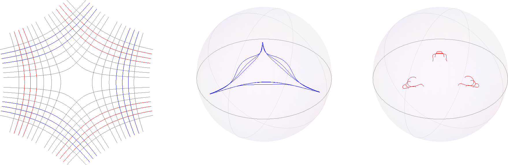
Figure 1. Left to right: Vertical and horizontal trajectories of $zdz^{2}$; the images of vertical trajectories under the Epstein-Schwarz map approximate an ideal triangle, as shown here in the unit ball model of $\mathbb{H}^{3}$; segments on horizontal trajectories are contracted to sets of small diameter.

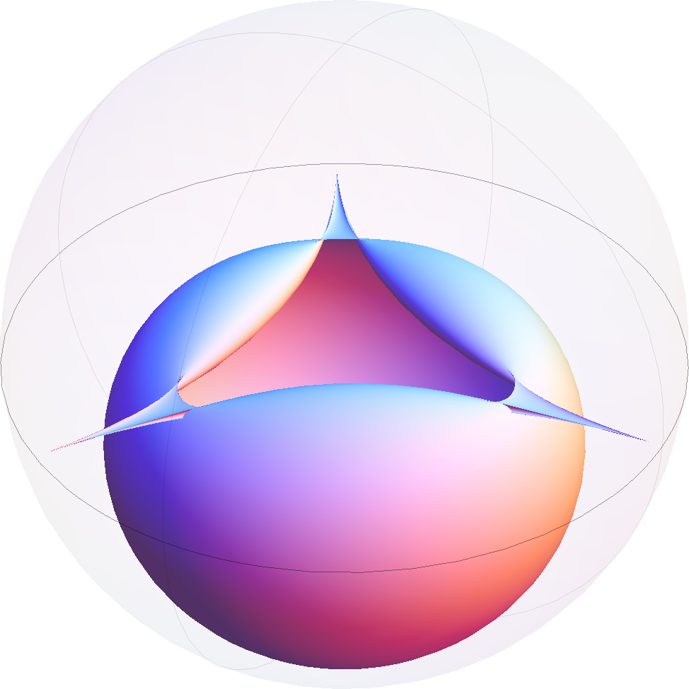
Figure 2. The image of a small neighborhood of the origin under the Epstein-Schwarz map of $zdz^{2}$ in the unit ball model of $\mathbb{H}^{3}$. The ideal point $(0,0,-1)$ corresponds to the image of $0$ under the developing map.

Example 2.

Next we consider $\phi=zdz^{2}$ on $\mathbb{C}$. While in this case it is possible to find closed-form expressions for the developing map (in terms of Airy functions) and for the Epstein-Schwarz map, we will only discuss the qualitative features seen in Figures 1–2. Here the origin is a simple zero of $\phi$ which corresponds to a cone point of angle $3\pi$ for the $\phi$-metric. Centered at the origin we can construct a regular right-angled geodesic hexagon of alternating vertical and horizontal sides. By Theorem 3.9, if this hexagon is far enough from the origin then the Epstein-Schwarz map sends its vertical sides to long near-geodesic segments in $\mathbb{H}^{3}$, while the horizontal sides are mapped to sets of small diameter. Thus the image of the hexagon itself approximates an ideal triangle. Note that avoiding a small neighborhood of the origin also ensures that the trajectories of $\phi=zdz^{2}$ are close to those of $\widehat{\phi}=(z+\frac{5}{8z^{2}})dz^{2}$, so the images of these curves approximate lines of curvature on the Epstein surface.

Near the origin (i.e. for small $d$) the behavior of the Epstein-Schwarz surface is quite different. A small punctured neighborhood of $0$ maps to the “bubble” shown in Figure 2—a properly embedded, infinite area surface whose induced metric is approximately isometric to $|\widehat{\phi}|/|\phi|^{1/2}\sim|z|^{-5/2}|dz|$ (by Lemma 3.3). The corresponding surface in $\mathbb{H}^{3}$ approaches the developed image of $0$ tangentially, eventually leaving every horoball based at that point.

4. Sequences of Epstein-Schwarz maps

In the previous section we considered the geometry of the Epstein-Schwarz map for a single complex projective structure on a surface. We now analyze how these results apply to a divergent sequence of projective structures whose associated quadratic differentials converge projectively. Specifically, throughout this section we assume:

(4.1) $$\begin{cases}(f_{n},\rho_{n})\text{ is a sequence of projective structures on }X\\ \phi_{n}\in Q(X)\text{ is the associated sequence of Schwarzian derivatives}\\ \phi_{n}\to\infty\text{ as }n\to\infty\\ \lim_{n\to\infty}\frac{\phi_{n}}{\|\phi_{n}\|}=\phi\end{cases}$$

The theme we develop is that the foliation and transverse measure of the projective limit $\phi$ governs the large-scale geometry of $\operatorname{\Sigma}_{\phi_{n}}$ for large $n$.

4.1. Nonsingular segments

Let $\tilde{\phi}$ and $\tilde{\phi}_{n}$ denote the lifts of $\phi$ and $\phi_{n}$ to $\tilde{X}$, and let $\tilde{Z}_{\phi}$ denote the set of zeros of $\tilde{\phi}$. By compactness of $X$ and the convergence of $\phi_{n}/\|\phi_{n}\|$ we have

(4.2) $$\frac{|\tilde{\phi_{n}}-\tilde{\phi}|}{|\tilde{\phi}|}\to 0$$

uniformly on compact subsets of $\tilde{X}-\tilde{Z}_{\phi}$.

Theorem 4.1.

Let $I\subset\tilde{X}$ denote a nonsingular and non-horizontal $\phi$-geodesic segment. Then there exists $N>0$ and sequences $K_{n}\to 1$ and $C_{n}\to 0$ as $n\to\infty$ such that for each $n>N$ and any $x_{0},x_{1}\in I$ with $\phi$-height difference $h$, we have

(4.3) $$K_{n}^{-1}\|2\phi_{n}\|^{1/2}h-C_{n}\leqslant d_{\mathbb{H}^{3}}(\operatorname{\Sigma}_{\phi_{n}}(x_{0}),\operatorname{\Sigma}_{\phi_{n}}(x_{1}))\leqslant K_{n}\|2\phi_{n}\|^{1/2}h+C_{n}.$$

The constants $N,K_{n},C_{n}$ can be taken to depend only on $\phi_{n}$ and $d_{\phi}(I,Z_{\phi})$. Furthermore, the same estimate holds for any non-horizontal half- or bi-infinite geodesic $I$ with the property that $d_{\phi}(J,Z_{\phi})>0$.

Before starting the proof, we remark that since the quantity $\|2\phi_{n}\|^{1/2}h$ appearing in this estimate exactly the $(2\|\phi_{n}\|\phi)$-height of $I$, an equivalent statement is that the $(2\|\phi_{n}\|\phi)$-height parameterization of $I$ maps to a quasigeodesic in $\mathbb{H}^{3}$ with constants $(K,C)$ converging to $(1,0)$ as $n\to\infty$.

Proof.

Let $L^{(1)}$ denote the length of a subsegment of $I$ that has height $1$. Let $J\subset I$ denote a subsegment of length $L<L^{(1)}$, which therefore has height $L/L^{(1)}$.

Let $U$ denote the $d/2$-neighborhood of $J$ in the $\phi$-metric, where $d=d_{\phi}(J,Z_{\phi})$. Let $\phi_{n}^{0}=\phi_{n}/\|\phi_{n}\|$. By uniform convergence of the differentials $\phi_{n}^{0}$, for each $k\in\mathbb{N}$ there exists $N(k)\in\mathbb{N}$ such that for $n>N(k)$ we can apply Lemma 2.4 to $J$ and $U$ with $\delta=d/(16kL^{(1)})$. Thus for such $n$ there is a $\phi_{n}^{0}$-geodesic segment with endpoints $\{x_{0},x_{1}\}$, and we have

(4.4) $$\begin{split}\max(|L_{n}^{0}-L|,|h_{n}^{0}-h|)&<\frac{dL}{4kL^{(1)}}=\frac{dh}{4k}\\ d_{\phi_{n}^{0}}(J^{\prime},Z_{\phi_{n}})\geqslant d_{\phi_{n}^{0}}(J^{\prime},\partial U)&>\frac{d}{8}\end{split}$$

where $L_{n}^{0}$ and $h_{n}^{0}$ are the $\phi_{n}^{0}$-length and height of the $\phi_{n}^{0}$-geodesic segment $J^{\prime}$ with endpoints $\{x_{0},x_{1}\}$. Letting $L_{n}=\|\phi_{n}\|^{1/2}L_{n}^{0}$ and $h_{n}=\|\phi_{n}\|^{1/2}h_{n}^{0}$ denote the corresponding quantities for $J^{\prime}$ with respect to $\phi_{n}$, and writing $d_{n}:=d_{\phi_{n}}(J^{\prime},Z_{\phi_{n}})>\|\phi_{n}\|^{1/2}d/k$, we have

$$\frac{d_{n}}{\sqrt{L_{n}}}>\frac{\|\phi_{n}\|^{1/4}d}{8L_{n}^{0}}>\frac{\|\phi_{n}\|^{1/4}d}{8(L-d/(4k))}$$

again for all $k$ and $n>N(k)$. By taking $n$ and $k$ large enough it follows that $d_{n}$ and $d_{n}/\sqrt{L_{n}}$ can be made arbitrarily large.

For any $m>0$, let $N^{\prime}(m)$ be such that $d_{n}/(1+\sqrt{L_{n}})>m$ for all $n>N^{\prime}(m)$. Then for $m>M$ and $n>N^{\prime}(m)$ we apply Theorem 3.9 to $J^{\prime}$, concluding that

$$K^{\prime}(m)^{-1}\sqrt{2}\,h_{n}-C^{\prime}(m)<d_{\mathbb{H}^{3}}(\operatorname{\Sigma}_{\phi_{n}}(x_{0}),\operatorname{\Sigma}_{\phi_{n}}(x_{1}))<K^{\prime}(m)\sqrt{2}\,h_{n}+C^{\prime}(m).$$

Thus the parameterization of $J$ by $2\phi_{n}$-height is mapped by $\operatorname{\Sigma}_{\phi_{n}}$ to a $(K^{\prime}(m),C^{\prime}(m))$-quasigeodesic. Note that the $2\phi_{n}$-height of $J$ tends to $\infty$ as $n\to\infty$.

If the length of $I$ is greater than $L^{(1)}$ (e.g. if it is a ray or infinite geodesic), then for $n$ sufficiently large we can apply Lemma 3.8 to $J$ and conclude that in any case, the $2\phi_{n}$-height parameterization of $I$ maps to a $(K^{\prime\prime}(m),C^{\prime\prime}(m))$-quasigeodesic, where $(K^{\prime\prime}(m),C^{\prime\prime}(m))\to(1,0)$ as $m\to\infty$.

Finally we must consider the effect of changing from the $2\phi_{n}$-height parameterization to the $2\phi$-height. For the remainder of the proof let $x_{0},x_{1}\in I$ be an arbitrary pair of points and let $L$ denote the $\phi$-length of the segment $[x_{0},x_{1}]\subset I$. Note that it is no longer assumed that $L<L^{(1)}$.

By applying (4.4) $\lceil L/L^{(1)}\rceil$ times we conclude that the $\phi_{n}$-height differences $h_{n}$ and $\phi$-height difference $h$ between $x_{0}$ and $x_{1}$ satisfy

$$|\sqrt{2}\,h_{n}-\|2\phi\|^{1/2}h|<\frac{\|2\phi_{n}\|^{1/2}dL}{4kL^{(1)}}=\left(\frac{d}{4k}\right)\|2\phi_{n}\|^{1/2}h,$$

where in the last step we have used that $L/L^{(1)}=h$. Therefore, changing from the $2\phi_{n}$-height to the $(\|2\phi_{n}\|\phi)$-height parameterization of $I$ introduces a multiplicative error in the distance estimate that is $o(\|\phi_{n}\|^{1/2}h)$ as $k\to\infty$, and (4.3) follows with

$$\begin{split}N&=N^{\prime}(M),\\ K_{n}&=K^{\prime\prime}(m_{0}(n))+d/4k_{0}(n),\\ C_{n}&=C^{\prime\prime}(m_{0}(n)),\\ \end{split}$$

where

$$\begin{split}k_{0}(n)&=\max\{k\>|\>N(k)<n\},\\ m_{0}(n)&=\max\{m\>|N^{\prime}(m)<n\}.\\ \end{split}$$

∎

Complementing Theorem 4.1 we have the following estimate for horizontal segments:

Theorem 4.2.

Let $I\subset\tilde{X}$ denote a nonsingular $\phi$-horizontal segment. Then we have

$$\operatorname{Diam}(\operatorname{\Sigma}_{\phi_{n}}(I))=o(\|\phi_{n}\|^{1/2})\text{ as }n\to\infty.$$

As with Theorem 4.1, the above estimate for the geometry of the image is not uniform—it depends on the particular segment $I$.

Proof.

We proceed in much the same way as the previous proof, but using the whole segment instead of a subsegment of height $1$.

Denote by $L_{n}$ the $\phi_{n}$-length of the $\phi_{n}$-geodesic $I^{\prime}$ with the same endpoints as $I$ and by $d_{n}$ the $\phi_{n}$-distance from $I^{\prime}$ to $Z_{\phi_{n}}$. For large $n$ we can apply Lemma 2.4 to a $d/2$-neighborhood $I$ in the $\phi$-metric with $\delta=d/(16kL)$, where $L$ is the $\phi$-length of $I$. Then as in the previous proof we have $m_{n}\to\infty$ as $n,k\to\infty$, where

$$m_{n}:=\frac{d_{n}}{1+\sqrt{L_{n}}}.$$

We also have $h_{n}^{0}<\frac{d}{4k}$, or equivalently, $\sqrt{2}\,h_{n}<d\|2\phi_{n}\|^{1/2}/(4k)$.

Let $x_{0},x_{1}$ be the endpoints of $I$, which are also the endpoints of $I^{\prime}$. Applying Corollary 3.10 if $I^{\prime}$ is $\phi_{n}$-horizontal, and Theorem 3.9 if it is not, we conclude

$$\begin{split}d_{\mathbb{H}^{3}}(\operatorname{\Sigma}_{\phi_{n}}(x_{0}),\operatorname{\Sigma}_{\phi_{n}}(x_{1}))&\leqslant K^{\prime}(m_{n})\sqrt{2}\,h_{n}+C^{\prime}(m_{n})\\ &\leqslant\frac{K^{\prime}(m)d}{4k}\|2\phi_{n}\|^{1/2}+C^{\prime}(m_{n}),\end{split}$$

for $n>N(k)$, and using $k=k_{0}(n)$ as in the proof of Theorem 4.1 we find that the right hand side is $o(\|\phi_{n}\|^{1/2})$ as $n\to\infty$.

Finally, we note that a subsegment of $I$ is shorter and its distance from $Z_{\phi}$ is no less than that of $I$. Decreasing $L$ and increasing $d$ preserve (or improve) all of the estimates above, so the distance estimate above applies to all pairs $x_{0},x_{1}\in I$. This gives the desired bound on the diameter of $\operatorname{\Sigma}_{\phi_{n}}(I)$. ∎

4.2. Periodic geodesics

Given an element $g\in\operatorname{\mathrm{SL}}_{2}\mathbb{C}$ let

$$\ell(g)=\inf_{x\in\mathbb{H}^{3}}d(x,g\cdot x)$$

denote its translation length when acting as an isometry of $\mathbb{H}^{3}$. Thus $\ell(g)>0$ if and only if $g$ is a hyperbolic element, in which case $g$ translates along its geodesic axis by distance $\ell(g)$.

Theorem 4.3.

If $\gamma\in\Pi$ is represented by a periodic $\phi$-geodesic of height $h$, then

(4.5) $$\lim_{n\to\infty}\frac{\ell(\rho_{n}(\gamma))}{\|2\phi_{n}\|^{1/2}}=h.$$

In particular if $h>0$ then $\rho_{n}(\gamma)$ is hyperbolic for all sufficiently large $n$.

Proof.

Recall that $\operatorname{\Sigma}_{\phi_{n}}(\gamma\cdot x)=\rho_{n}(\gamma)\cdot\operatorname{\Sigma}_{\phi_{n}}(x)$.

First suppose $h>0$. Applying Theorem 4.1 to a nonsingular $\tilde{\phi}$-geodesic axis of $\gamma$ in $\tilde{X}$, we find that $\rho_{n}(\gamma)$ preserves a $(K_{n},C_{n})$-quasigeodesic axis in $\mathbb{H}^{3}$ along which it moves points distance $d_{n}$, where

$$K_{n}^{-1}\|2\phi_{n}\|^{1/2}h-C_{n}<d_{n}<K_{n}^{-1}\|2\phi_{n}\|^{1/2}h+C_{n}.$$

By Lemma 3.7, this quasigeodesic axis lies in a uniformly bounded neighborhood of the geodesic axis of $\rho_{n}(\gamma)$. The translation length of $\ell(\rho_{n}(\gamma))$ is therefore $d_{n}+O(1)$ as $n\to\infty$, and since $(K_{n},C_{n})\to(1,0)$, the desired estimate follows.

If $h=0$ then we apply Theorem 4.2 to the horizontal $\tilde{\phi}$-geodesic fixed by $\gamma$ to get a pairs of points in $\mathbb{H}^{3}$ related by $\rho_{n}(\gamma)$ and separated by distance $o(\|\phi_{n}\|^{1/2})$. This distance is an upper bound for $\ell(\rho_{n}(\gamma))$ hence $\lim_{n\to\infty}\frac{\ell(\rho_{n}(\gamma))}{\|2\phi_{n}\|^{1/2}}=0$ as required. ∎

5. The character variety and growth rates

In this section we show how the results and techniques of Sections 3–4 can be used to study the growth rate of the holonomy representation as a function of the Schwarzian.

5.1. The character variety and holonomy map

The $\operatorname{\mathrm{SL}}_{2}(\mathbb{C})$-representation variety of $\Pi$ is the set $\mathcal{R}(\Pi)=\operatorname{Hom}(\Gamma,\operatorname{\mathrm{SL}}_{2}(\mathbb{C}))$. Choosing a finite generating set $\Sigma$ for $\Pi$ realizes $\mathcal{R}(\Pi)$ as a closed algebraic subset of $(\operatorname{\mathrm{SL}}_{2}(\mathbb{C}))^{|\Sigma|}$, giving it the structure of an algebraic variety.

The $\operatorname{\mathrm{SL}}_{2}(\mathbb{C})$-character variety of $\Pi$, denoted $\mathcal{X}(\Pi)$, is an affine algebraic variety consisting of the characters (traces) of representations in $\mathcal{R}(\Gamma)$; there is a natural algebraic map $\mathcal{R}(\Gamma)\to\mathcal{X}(\Gamma)$ taking a representation to its character. We denote this map by $\rho\mapsto[\rho]$. The character variety can also be described as an algebraic quotient

$$\mathcal{X}(\Gamma)=\mathcal{R}(\Gamma)/\!\!/\operatorname{\mathrm{SL}}_{2}(\mathbb{C})$$

where $\operatorname{\mathrm{SL}}_{2}(\mathbb{C})$ acts by conjugating representations. See [CS] and [MS1, Sec. II.4] for details about these constructions.

As mentioned in the introduction, there is holomorphic map

$$\operatorname{hol}:Q(X)\to\mathcal{X}(\Pi),$$

the holonomy map, which associates to a projective structure on $X$ the character of its holonomy representation (which is well-defined, since the representation itself is well-defined up to conjugation).

5.2. Properness

Gallo, Kapovich, and Marden showed that the holonomy map $Q(X)\to\mathcal{X}(\Pi)$ is a proper map [GKM, Thm. 11.4.1], following an outline presented in [Kap1, Sec. 7.2]. A geometric approach to properness using pleated surfaces can be found in [Tan2]. The same result also follows easily from Theorem 4.3:

Theorem 5.1.

The map $\operatorname{hol}:Q(X)\to\mathcal{X}(\Pi)$ is proper.

Proof.

Let $\phi_{n}\in Q(X)$ be a divergent sequence. By passing to a subsequence we can assume that $\phi_{n}$ converges projectively, i.e. $\phi_{n}/\|\phi_{n}\|\to\phi$. Let $\gamma\in\Pi$ be freely homotopic to a periodic $\phi$-geodesic. The translation length of the image of $\gamma$ under a representation $\rho:\Pi\to\operatorname{\mathrm{SL}}_{2}(\mathbb{C})$ defines a continuous function $\ell_{\gamma}:\mathcal{X}(\Pi)\to\mathbb{R}$. By Theorem 4.3 we have $\ell_{\gamma}(\operatorname{hol}(\phi_{n}))\to\infty$, so the image of the sequence $\{\operatorname{hol}(\phi_{n})\}$ is not contained in a compact set. ∎

5.3. Growth estimate

This approach to proving properness of the holonomy map also lends itself to effective estimates of the growth rate of holonomy representations. In fact, Theorem 4.3 can be seen as an estimate of this kind, where translation length of the action on $\mathbb{H}^{3}$ is used to measure the “size” of a representation. Since translation length grows logarithmically with respect to trace coordinates on $X(\Pi)$, the holonomy map itself has exponential growth in these coordinates. Making this coordinate-independent, we have the following:

Theorem 5.2 (Effective properness).

For any affine embedding $\mathcal{X}(\Pi)\hookrightarrow\mathbb{C}^{n}$ and any norm $\|{\mathchoice{\mkern 1.0mu\mbox{\raise 2.2pt\hbox{$\centerdot$}}\mkern 1.0mu}{\mkern 1.0mu\mbox{\raise 2.2pt\hbox{$\centerdot$}}\mkern 1.0mu}{\mkern 1.5mu\centerdot\mkern 1.5mu}{\mkern 1.5mu\centerdot\mkern 1.5mu}}\|$ on $\mathbb{C}^{n}$ there are constants $A>0$ and $B$ such that

(5.1) $$A^{-1}\|\phi\|^{1/2}-B<\log(1+\|\operatorname{hol}(\phi)\|)<A\|\phi\|^{1/2}+B.$$

In [Sim], Simpson uses harmonic maps techniques to obtain a similar bound for the growth rate of the map from the de Rham moduli space of rank-$2$ systems of ordinary differential equations over a compact Riemann surface to the character variety of the fundamental group. It would be interesting to know whether the set of projective structures is properly embedded in this moduli space of ODEs, and thus to see if the growth rate of holonomy in terms of the norm of the Schwarzian can also be estimated by Simpson’s technique.

The proof of Theorem 5.2 will depend on an estimate that is a direct analog of Theorem 4.3, but where we consider a fixed homotopy class of curves and an arbitrary quadratic differential, instead of a fixed sequence of quadratic differentials and an arbitrary homotopy class.

Theorem 5.3.

For each $\gamma\in\Pi$ there exists constants $C>0$ and $N>0$ such that if $\phi\in Q(X)$ satisfies $\|\phi\|>N$ then

$$\ell(\rho_{\phi}(\gamma))\leqslant C\|\phi\|^{1/2}.$$

Furthermore, if $\gamma$ is represented by a periodic $\phi$-geodesic of height $h$, angle $\theta>0$, and whose associated flat annulus has width at least $w\|\phi\|^{1/2}$, then

$$\ell(\rho_{\phi}(\gamma))\geqslant c\|\phi\|^{1/2},$$

where in this case $c$ and $N$ also depend on $\gamma$, $\theta$, and $w$.

Proof.

The unit sphere in $Q(X)$ corresponds to a compact family of metrics on $X$. Thus the free homotopy class of an element $\gamma\in\Pi$ can be realized by a curve of uniformly bounded length and height with respect to any $\phi$ such that $\|\phi\|=1$. Increasing length and height by a bounded amount we can further assume that each such realization avoids a fixed neighborhood of $Z_{\phi}$.

Scaling to obtain $\phi\in Q(X)$ of any norm, we conclude that $\gamma$ is represented by a closed curve in $X$ of length bounded by $C^{\prime}\|\phi\|^{1/2}$ and which avoids a $\delta\|\phi\|^{1/2}$-neighborhood of $Z_{\phi}$, for some constants $C^{\prime},\delta$. We can lift this closed curve to a path in $\tilde{X}$ whose endpoints are identified by the action of $\gamma$. Choosing $N$ large enough we can apply Lemma 3.6 to conclude that $\operatorname{\Sigma}_{\phi}$ is uniformly Lipschitz on this path, so the image in $\mathbb{H}^{3}$ has length bounded by $C^{\prime\prime}\|\phi\|^{1/2}$. Since the endpoints of the image are identified by $\rho_{\phi}(\gamma)$, this gives the desired upper bound for $\ell(\rho_{\phi}(\gamma))$.

For the periodic case we can again use compactness of the unit sphere in $Q(X)$ and the angle $\theta$ to obtain a lower bound on the $\phi$-height of a periodic geodesic homotopic to $\gamma$ of the form $h>c^{\prime}\|\phi\|^{1/2}$, where $c^{\prime}$ depends on $\gamma$ and $\theta$. Of course the length estimate $L<C^{\prime}\|\phi\|^{1/2}$ applies as above. Using the geodesic representative in the center of the flat annulus, the distance from this geodesic to the nearest zero of $\phi$ is at least $d=\frac{1}{2}w\|\phi\|^{1/2}$.

For $\|\phi\|>N$ and $N$ sufficiently large (now depending on $\gamma$, $\theta$, and $w$), we have $d>M(1+\sqrt{L})$ where $M$ is the constant from Theorem 3.9. Then (3.10) shows that the lift of the periodic geodesic to $\tilde{X}$ maps by $\operatorname{\Sigma}_{\phi}$ to a uniformly quasigeodesic axis for $\rho_{\phi}(\gamma)$ in $\mathbb{H}^{3}$ on which the translation length is bounded below by a multiple of the height $h$. Using the stability of quasigeodesics in $\mathbb{H}^{3}$ (Lemma 3.7) we obtain a lower bound of the form $\ell(\rho_{\phi}(\gamma))>c^{\prime\prime}\|\phi\|-D$. The lower bound on $\|\phi\|$ allows us to remove the additive constant by changing the multiplicative factor slightly, and the Theorem follows. ∎

Proof of Theorem 5.2..

Let $P\subset\Pi$ and $w_{0}$ be as in Theorem 2.2. Since traces of elements of $\Pi$ are regular functions on $\mathcal{X}(\Pi)$, the traces of elements of $P$ have a uniformly polynomial upper bound in the coordinates of the affine embedding. Thus there are constants $C,k$ such that for all $\gamma\in P$ we have

$$|\operatorname{Tr}(\rho_{\phi}(\gamma))|\leqslant C(1+\|\operatorname{hol}(\phi)\|)^{k}.$$

For each $\phi\in Q(X)$ there exists $\gamma\in P$ that is represented by a periodic $\phi$-geodesic that is nearly vertical and thus has height bounded below by $c\|\phi\|^{1/2}$ for some positive constant $c$. Since we also have a uniform lower bound on the widths of the corresponding flat annuli, Theorem 5.3 and the relation between trace and translation length give

$$|\operatorname{Tr}(\rho_{\phi}(\gamma))|>\exp(c^{\prime}\|\phi\|^{1/2})$$

for some $c^{\prime}>0$, as long as $\|\phi\|>M$. Here we have uniform constants because $P$ is finite. Combining this with the previous inequality and taking logarithms gives the lower bound on $\|\operatorname{hol}(\phi)\|$ from (5.1), where adjusting the additive constant $B$ allows us to remove the requirement that $\|\phi\|$ is large.

The upper bound from (5.1) is similar, but easier: The ring of regular functions on $\mathcal{X}(\Pi)$ is generated by the trace functions of finitely many elements of $\Pi$ (see [CS, Sec. 1.4]), so $\|\operatorname{hol}(\phi)\|$ has a polynomial upper bound in terms of these traces. Applying the upper bound on translation length from Theorem 5.3 to these elements and again taking logarithms completes the proof. ∎

6. The Morgan-Shalen compactification and straight maps

6.1. The compactification

Consider the map $\mathcal{X}(\Pi)\to(\mathbb{R}^{+})^{\Pi}$ given by

$$[\rho]\mapsto\left(\log(|\operatorname{Tr}\rho(\gamma)|+2)\right)_{\gamma\in\Pi}.$$

Let $\mathbb{P}(\mathbb{R}^{+})^{\Pi}$ denote the space of rays in $(\mathbb{R}^{+})^{\Pi}$ and consider the projectivized map $\mathcal{X}(\Pi)\to\mathbb{P}(\mathbb{R}^{+})^{\Pi}$. The image of $\mathcal{X}(\Pi)$ is precompact and the closure of the image defines the Morgan-Shalen compactification of $\mathcal{X}(\Pi)$. If $\ell:\Pi\to\mathbb{R}^{+}$ is a function whose projective class $[\ell]$ is a boundary point of $\mathcal{X}(\Pi)$, then there exists an $\mathbb{R}$-tree $T$ and an isometric action of $\Pi$ on $T$ such that

$$\ell(\gamma)=\inf_{x\in T}d(x,\gamma\cdot x),$$

that is, $\ell$ is the translation length function of an action of $\Pi$ on an $\mathbb{R}$-tree. As in the introduction we say in this case that $T$ represents $[\ell]$.

This compactification was introduced in [MS1] where a tree representing a boundary point is described in terms of a valuation on the function field of $\mathcal{X}(\Pi)$. For our purposes it will be important to construct such a tree directly from the action of a representation on hyperbolic space, so we will use an alternative construction of representing trees based on the asymptotic cone.

6.2. Asymptotic cone construction

Bestvina [B] and Paulin [Pau] used geometric limit constructions to build $\mathbb{R}$-trees representing limit points of sequences of representations in the Morgan-Shalen compactification. Later, Chiswell [Chi] and Kapovich-Leeb [KL] described how these limit constructions can be interpreted in terms of asymptotic cones of hyperbolic spaces. We now review this approach, mostly following the exposition of [Kap2, Ch. 9–10].

Fix a non-principal ultrafilter $\omega$ on $\mathbb{N}$ and denote by $\operatorname{\lim_{\omega}}a_{n}$ the $\omega$-limit of a sequence of real numbers $\{a_{n}\}$. Given a metric space $X$, a sequence of points $c_{n}\in X$, and a sequence $\epsilon_{n}\to 0$ of positive reals, we denote by

$$\operatorname{\lim_{\omega}}\>(\epsilon_{n}X,c_{n})$$

the asymptotic cone of $X$ based at $x_{n}$ with scale factors $\epsilon_{n}$; this is the quotient metric space associated with the set of sequences

$$\{x=(x_{n})\>|\>x_{n}\in X,\;\operatorname{\lim_{\omega}}\epsilon_{n}d(c_{n},x_{n})<\infty\}$$

and the pseudometric

$$d(x,y)=\operatorname{\lim_{\omega}}\epsilon_{n}d(x_{n},y_{n}).$$

If $X$ is a $\mathrm{CAT}(\kappa)$ space for some $\kappa<0$ (for example, $X=\mathbb{H}^{3}$) then $\operatorname{\lim_{\omega}}\>(\epsilon_{n}X,c_{n})$ is an $\mathbb{R}$-tree.

Now fix a finite generating set $\Sigma$ for $\Pi$. If $\rho:\Pi\to\operatorname{Isom}(X)$ is an isometric action, we define the local scale of $\rho$ at $x$ to be the quantity

$$R(\rho,x)=\max_{\gamma\in\Sigma}d(x,\rho(\gamma)\cdot x).$$

Specializing to the case of $X=\mathbb{H}^{3}$, the basic link between the asymptotic cone construction and the Morgan-Shalen compactification is the following (see [Kap2, Sec. 10.4]):

Theorem 6.1.

Consider a sequence $\rho_{n}\in\mathcal{X}(\Pi)$ and identify it with a sequence of isometric actions of $\Pi$ on $\mathbb{H}^{3}$ using the covering $\operatorname{\mathrm{SL}}_{2}\mathbb{C}\to\operatorname{\mathrm{PSL}}_{2}\mathbb{C}\simeq\operatorname{Isom}^{+}(\mathbb{H}^{3})$. Let $c_{n}\in\mathbb{H}^{3}$ be a sequence of points and $\epsilon_{n}\to 0$ a sequence of positive reals.

1. If $\operatorname{\lim_{\omega}}\epsilon_{n}R(\rho_{n},x_{n})<\infty$, then the action

   $$\gamma:(x_{n})\mapsto(\rho_{n}(\gamma)\cdot x_{n})$$

   of $\Pi$ on sequences in $\mathbb{H}^{3}$ induces an isometric action of $\Pi$ on the $\mathbb{R}$-tree $T:=\operatorname{\lim_{\omega}}\>(\epsilon_{n}\mathbb{H}^{3},c_{n})$.

2. If the action of $\Pi$ on $T$ does not have a global fixed point, and if the sequence $[\rho_{n}]$ converges in the Morgan-Shalen compactification, then $T$ represents the Morgan-Shalen limit.

∎

The result above is proved in [Kap2, Sec. 10.4], though the statements of the theorems in that section are structured somewhat differently from the one above. Kapovich makes a specific choice of basepoints $c_{n}$, but this choice is only used to show the resulting action has no global fixed point, which we do not claim here. (That an arbitrary sequence of basepoints can be used is also established in [B, Prop. 4.8].) Similarly, while Kapovich fixes $\epsilon_{n}=R(\rho_{n},c_{n})^{-1}$, the arguments use only that $\operatorname{\lim_{\omega}}\epsilon_{n}R(\rho_{n},x_{n})<\infty$.

A key feature of this construction of a limit tree is that it gives a notion of convergence of a sequence $x_{n}\in\mathbb{H}^{3}$ to a point in $T$, which is simply a restatement of the definition: A point $x_{\infty}\in T$ is an equivalence class of sequences in $\mathbb{H}^{3}$, and we say $x_{n}\to x_{\infty}$ if the sequence $(x_{n})$ lies in that equivalence class. This allows us to consider the question of whether a sequence of maps into $\mathbb{H}^{3}$ converges pointwise to a map into $T$.

6.3. Convergence of Epstein-Schwarz maps

We return to the hypotheses of (4.1), that is, considering a divergent sequence of projective structures with holonomy representations $\rho_{n}$ and quadratic differentials $\phi_{n}$ converging projectively to $\phi$. We suppose also that $[\rho_{n}]$ converges in the Morgan-Shalen compactification to the projective equivalence class $[\ell]$ of a function $\ell:\Pi\to\mathbb{R}^{+}$.

Recall also that $\tilde{Z}_{\phi}\subset\tilde{X}$ is the discrete subset of the universal cover of $X$ consisting of points that project to zeros of $\phi$, and similarly for $\tilde{Z}_{\phi_{n}}$ and $\phi_{n}$.

Theorem 6.2.

Fix a point $z_{0}\in\tilde{X}\setminus\tilde{Z}_{\phi}$ and use its $\operatorname{\Sigma}_{\phi_{n}}$-images as basepoints to construct the asymptotic cone

$$T=\operatorname{\lim_{\omega}}\>(\|2\phi_{n}\|^{-1/2}\mathbb{H}^{3},\operatorname{\Sigma}_{\phi_{n}}(z_{0})).$$

Then:

1. The sequence of maps $\operatorname{\Sigma}_{\phi_{n}}:\tilde{X}\setminus\tilde{Z}_{\phi_{n}}\to\mathbb{H}^{3}$ converges (pointwise) to a continuous map $\operatorname{\Sigma}_{\infty}:\tilde{X}\to T$.

2. For any pair of points $x,y\in\tilde{X}$ that are endpoints of a nonsingular $\tilde{\phi}$-geodesic segment of height $h$, the map $\operatorname{\Sigma}_{\infty}$ satisfies

   $$d(\operatorname{\Sigma}_{\infty}(x),\operatorname{\Sigma}_{\infty}(y))=h.$$

3. The sequence $\rho_{n}$ induces an isometric action of $\Pi$ on $T$ which represents the Morgan-Shalen limit $[\ell]$, and $\operatorname{\Sigma}_{\infty}$ is equivariant for this action.

Note that in statement (i) the domains of the maps $\operatorname{\Sigma}_{\phi_{n}}$ vary with $n$ so the limit is a priori only defined on

$$\liminf_{n\to\infty}\>(\tilde{X}\setminus\tilde{Z}_{\phi_{n}}),$$

which contains $\tilde{X}\setminus\tilde{Z}_{\phi}$ since $\phi_{n}/\|\phi_{n}\|\to\phi$. However we will show that the limit map on $\tilde{X}\setminus\tilde{Z}_{\phi}$ has a unique continuous extension to $\tilde{X}$.

Proof.

Suppose $z,z^{\prime}\in\tilde{X}\setminus\tilde{Z}_{\phi}$. Join these points by a polygonal path in $\tilde{X}\setminus\tilde{Z}_{\phi}$ that is a finite union of nonsingular $\phi$-geodesic segments. Applying Theorems 4.1 and 4.2 to the segments and using the triangle inequality we find

(6.1) $$\limsup_{n\to\infty}\|2\phi_{n}\|^{-1/2}d(\operatorname{\Sigma}_{\phi_{n}}(z),\operatorname{\Sigma}_{\phi_{n}}(z^{\prime}))\leqslant\bar{h}$$

where $\bar{h}$ is the sum of the $\phi$-heights of the segments. Furthermore, if there is only one segment then the limit exists and is equal to $\bar{h}$.

Applying this to $z^{\prime}=z_{0}$ it follows that $\operatorname{\lim_{\omega}}\|2\phi_{n}\|^{-1/2}d(\operatorname{\Sigma}_{\phi_{n}}(z),\operatorname{\Sigma}_{\phi_{n}}(z_{0}))$ is finite, thus the sequence $\operatorname{\Sigma}_{\infty}(z):=(\operatorname{\Sigma}_{\phi_{n}}(z))$ represents a point of the asymptotic cone $T$. This gives the desired pointwise limit map on $\tilde{X}\setminus\tilde{Z}_{\phi}$. Equality of the limit (6.1) in the one-segment case is exactly statement (ii).

The polygonal path chosen above can be taken to agree with the minimizing $\tilde{\phi}$-geodesic joining $z$ to $z^{\prime}$ except in an arbitrarily small neighborhood $\tilde{Z}_{\phi}$ where the polygonal path must make short detours to avoid the zeros. As a result, we can assume that $\bar{h}$ is as close as we like to the $\tilde{\phi}$-height of the minimizing geodesic, which is itself a lower bound for the $\tilde{\phi}$-distance from $z$ to $z^{\prime}$. Therefore, the estimate above also shows that the limit $\operatorname{\Sigma}_{\infty}:(\tilde{X}\setminus\tilde{Z}_{\phi})\to T$ is $1$-Lipschitz for that metric, and in particular continuous. Furthermore, the asymptotic cone $T$ is a complete metric space (see e.g. [BH, Lem. 5.53]) so the Lipschitz map $\operatorname{\Sigma}_{\infty}$ extends uniquely and continuously to the metric completion of its domain, which is $\tilde{X}$. Statement (i) follows.

From the asymptotic cone construction it is immediate that a limit of equivariant maps is equivariant, as long as the group action is defined on the asymptotic cone. Thus statement (iii) is exactly the conclusion of Theorem 6.1 once we establish the relevant hypotheses, i.e.

1. $\operatorname{\lim_{\omega}}\|2\phi_{n}\|^{-1/2}R(\rho_{n},\operatorname{\Sigma}_{\phi_{n}}(z_{0}))<\infty$

2. $\Pi$ acts on $T$ without global fixed points.

Estimate (1) follows from (6.1) since each element of the finite generating set for $\Pi$ can be represented by a polygonal path in $\tilde{X}\setminus\tilde{Z}_{\phi}$ based at $z_{0}$. The total height of this collection of paths is then a bound for $\limsup_{n\to\infty}\|2\phi_{n}\|^{-1/2}R(\rho_{n},\operatorname{\Sigma}_{\phi_{n}}(z_{0}))$ and thus for the $\omega$-limit as well. Hence $\Pi$ acts on $T$.

Now suppose for contradiction that there is a point $x\in T$ fixed by $\Pi$. Then $x$ is the equivalence class of a sequence $(x_{n})\subset\mathbb{H}^{3}$ such that $\operatorname{\lim_{\omega}}\|2\phi_{n}\|^{-1/2}d(x_{n},\rho_{n}(\gamma)\cdot x_{n})=0$ for all $\gamma\in\Pi$. Thus

$$\liminf_{n\to\infty}\|2\phi_{n}\|^{-1/2}\ell(\rho_{n}(\gamma))\leqslant\liminf_{n\to\infty}\|2\phi_{n}\|^{1/2}d(x_{n},\rho_{n}(\gamma)\cdot x_{n})=0.$$

But this contradicts Theorem 4.3 for any $\gamma\in\Pi$ which can be represented by a periodic and non-horizontal $\phi$-geodesic, and such elements exist by Theorem 2.1. This contradiction shows (2), completing the proof of statement (iii). ∎

6.4. Dual trees of quadratic differentials

Given a measured foliation of a surface, we can lift the foliation to the universal cover and consider the space of leaves; the transverse measure of the foliation induces a metric on this leaf space, making it an $\mathbb{R}$-tree on which $\Pi$ acts by isometries (see [MS2] [Kap2, Sec. 11.12] for details). Applying this construction to the horizontal foliation $\mathcal{F}(\phi)$ of a quadratic differential $\phi\in Q(X)$ gives the dual tree $T_{\phi}$. By construction we also have a projection map $\pi:\tilde{X}\to T_{\phi}$.

6.5. Straight maps

A nonsingular $|\phi|$-geodesic segment in $\tilde{X}$ of height $h$ maps by $\pi$ to a geodesic segment of length $h$ (or a point, if $h=0$) in $T_{\phi}$. We say that a segment in $T_{\phi}$ is nonsingular if it arises in this way. (Note that a nonsingular segment in $T_{\phi}$ might also arise as the image of a geodesic in $\tilde{X}$ that contains singularities, because a given path in $T_{\phi}$ can have many geodesic lifts through $\pi$.)

We say that a map $F:T_{\phi}\to T$ is straight if its restriction to every nonsingular segment in $T_{\phi}$ is an isometric embedding. Evidently an isometry is a straight map, though the converse does not hold (see e.g. Lemma 6.5 below). Because any segment in $T_{\phi}$ can be lifted to a path in $\tilde{X}$ that is piecewise geodesic, straight maps are morphisms of $\mathbb{R}$-trees in the sense of [Sko].

We will use the following criterion for recognizing straight maps:

Lemma 6.3.

Let $T$ be an $\mathbb{R}$-tree and $f:\tilde{X}\to T$ a continuous map such that for every nonsingular $\phi$-geodesic segment $J$ in $\tilde{X}$ with height $h$ and endpoints $x,y$, we have

(6.2) $$d(f(x),f(y))=h.$$

Then the map $f$ factors as $f=F\circ\pi$ where $F:T_{\phi}\to T$ is straight and $\pi:\tilde{X}\to T_{\phi}$ is the projection. Furthermore, if $f$ is equivariant with respect to an action of $\Pi$ on $T$, then $F$ is also equivariant.

Proof.

Condition (6.2) implies that $f$ it is constant on all nonsingular horizontal leaf segments. By continuity, it is also constant on segments of horizontal leaf segments with endpoints at zeros, and therefore on all horizontal leaves (including those which pass through zeros of $\phi$). By construction of $\pi:\tilde{X}\to T_{\phi}$ as a quotient map, this is equivalent to having a unique factorization $f=F\circ\pi$ where $F:T_{\phi}\to T$ is continuous.

The parameterization of a $\phi$-geodesic in $\tilde{X}$ by height maps by $\pi$ to a geodesic segment in $T_{\phi}$ parameterized by arc length. Thus (6.2) shows that $F$ is an isometric embedding when restricted to a nonsingular segment in $T_{\phi}$, i.e. the map $F$ is straight.

Equivariance of $F$ follows from that of $f$ by uniqueness of the factorization. ∎

6.6. Proof of Theorem A

We have a divergent sequence $\phi_{n}$ with projective limit $\phi$ and an accumulation point $[\ell]$ of $\operatorname{hol}(\phi_{n})$ in the Morgan-Shalen boundary of $\mathcal{X}(\Pi)$. Pass to a subsequence (still called $\phi_{n}$) so that $\operatorname{hol}(\phi_{n})$ converges to $[\ell]$. Theorem 6.2 gives an $\mathbb{R}$-tree representing $[\ell]$, which we denote by $T_{0}$, and an equivariant map $\operatorname{\Sigma}_{\infty}:\tilde{X}\to T_{0}$. Let $T=\operatorname{\Sigma}_{\infty}(\tilde{X})$ denote the image of this map, which by equivariance is also an $\mathbb{R}$-tree carrying an isometric action of $\Pi$. Passing to an invariant subtree does not change the translation length function of a group action ([MS1, II.2.2 and II.2.12]), so $T$ also represents $[\ell]$. Part (ii) of Theorem 6.2 shows that the surjective map $\operatorname{\Sigma}_{\infty}:\tilde{X}\to T$ satisfies the hypotheses of Lemma 6.3 and hence gives a surjective, equivariant straight map $T_{\phi}\to T$. ∎

6.7. Simple zeros

For dual trees of quadratic differentials with only simple zeros, straight maps are isometric:

Lemma 6.4.

If $\phi\in Q(X)$ has only simple zeros, then any straight map $F:T_{\phi}\to T$ is an isometric embedding. In particular, if $\Pi$ acts minimally on $T$ and $F$ is equivariant, then $T$ is equivariantly isometric to $T_{\phi}$.

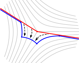
Figure 3. A geodesic passing through a simple zero can be pushed to a nonsingular segment by an isotopy that moves along leaves of the horizontal foliation.

The proof rests on a well-known technique of deforming a $\phi$-geodesic so that it avoids a neighborhood of the zeros (compare e.g. [Wol1, Lem. 4.6]), which for simple zeros can be accomplished without changing the image in the dual tree. The specific construction we use here closely parallels that of Farb-Wolf in [FW, Sec. 5.2].

Proof.

A local homeomorphism from an interval in $\mathbb{R}$ to an $\mathbb{R}$-tree is in fact a homeomorphism and its image is a geodesic. Consider a pair of points $x,y\in T_{\phi}$ and lifts $\tilde{x},\tilde{y}\in\tilde{X}$ through the projection $\pi:\tilde{X}\to T_{\phi}$. Let $J$ be the $\phi$-geodesic joining $\tilde{x}$ and $\tilde{y}$, which consists of a sequence of nonsingular segments that meet at zeros of $\phi$.

Since $F$ is straight, its restriction to $\pi(J)$ maps each nonsingular segment onto a geodesic in $T$, and the sum of the lengths of these geodesics is $d(x,y)$. If we show that $\left.F\right|_{\pi(J)}$ is also locally injective near the image of a zero of $\phi$, then $f(J)$ is the geodesic from $f(x)$ to $f(y)$ and we conclude that $d(x,y)=d(f(x),f(y))$ for all $x,y\in T$.

If a $\phi$-geodesic $J\subset\tilde{X}$ passes through a zero $z$ of $\phi$, then sum of the angles on either side of $J$ at $z$ is $(k+2)\pi$, where $k$ is the order of the zero. Thus at a simple zero, there is a side on which the angle is less than $2\pi$. On this side, we can push the part of $J$ near $z$ to a nonsingular segment of a vertical leaf by an isotopy that moves along horizontal leaves of $\phi$ (see Figure 3). In particular the segment of $\pi(J)$ near $\pi(z)$ is also the image of a nonsingular segment in $\tilde{X}$. Since a straight map is injective on such segments, we conclude that $\left.F\right|_{\pi(J)}$ is locally injective, as desired. ∎

6.8. Proof of Theorem B

Let $[\ell]$ be an accumulation point of $\operatorname{hol}(\phi_{n})$. Theorem A gives a tree $T$ representing $[\ell]$ and a straight map $T_{\phi}\to T$. By Lemma 6.4 the straight map is an isometric embedding and hence $[\ell]$ is the length function of the action of $\Pi$ on $T_{\phi}$. In particular there is only one accumulation point of this sequence in the Morgan-Shalen compactification. Furthermore, by [CM, Thm. 3.7], any $\mathbb{R}$-tree on which $\Pi$ acts isometrically with this length function has a unique minimal invariant subtree equivariantly isometric to $T_{\phi}$.

The set of quadratic differentials that have a zero of multiplicity at least $2$ is a closed algebraic subvariety of $Q(X)\simeq\mathbb{C}^{3g-3}$, so this set is nowhere dense and null for the Lebesgue measure class. This gives the required properties for the set of differentials with only simple zeros. ∎

6.9. Abelian actions and straight maps

An abelian action of $\Pi$ on an $\mathbb{R}$-tree is one which has nonzero translation length function $\ell:\Pi\to\mathbb{R}$ of the form $\ell(g)=|\chi(g)|$ where $\chi:\Pi\to\mathbb{R}$ is a homomorphism. (See [AB] for detailed discussion of such actions.) The homomorphism $\chi$ can be recovered, up to sign, from the length function $\ell$. The action of $\Pi$ on $\mathbb{R}$ by translations given by $g\cdot x=x+\chi(g)$, is an example of an abelian action, which we call the shift induced by $\chi$.

An abelian action on an $\mathbb{R}$-tree fixes an end of the tree, and the Busemann function of this end gives an equivariant map $b:T\to\mathbb{R}$ that intertwines the action of $\Pi$ on $T$ with the shift induced by $\chi$. Thus the shift is “final” among actions with a given abelian length function.

Straightness is also preserved by composition with the Busemann function of an abelian action:

Lemma 6.5.

Let $T$ be an $\mathbb{R}$-tree equipped with an abelian action of $\Pi$ by isometries, and let $b:T\to\mathbb{R}$ denote the Busemann function of a fixed end. If $F:T_{\phi}\to T$ is an equivariant straight map, then $b\circ F$ is also straight.

Proof.

Let $\gamma\in\Pi$ be an element represented by a periodic $\phi$-geodesic. This periodic geodesic lifts to a complete geodesic axis $\tilde{L}\subset\tilde{X}$ on which $\gamma$ acts as a translation, and $L:=\pi(L)\subset T_{\phi}$ is the axis of the action of $\gamma$ on $T_{\phi}$.

Because $F$ is $\phi$-straight, it maps $L$ homeomorphically to the geodesic axis of $\gamma$ in $T$. Since $F(L)$ is $\gamma$-invariant, in one direction it is asymptotic to the fixed end of $\Pi$ on $T$, and the restriction of $b$ to $F(L)$ is an isometry. Thus $b\circ f$ maps any segment along $L$ of height $h$ to an interval in $\mathbb{R}$ of length $h$.

Now consider an arbitrary nonsingular $\phi$-geodesic segment $J\subset\tilde{X}$ with endpoints $\tilde{x},\tilde{y}$ and height $h$. By Theorem 2.1, periodic $\phi$-geodesics are dense in the unit tangent bundle of $X$, so we can approximate $J$ by a segment on an axis of some element $\gamma\in\Pi$ in $\tilde{X}$. More precisely, we can find such $\tilde{L}$ and a pair of points $\tilde{x}^{\prime},\tilde{y}^{\prime}\in\tilde{L}$ such that the pairs $(\tilde{x},\tilde{x}^{\prime})$ and $(\tilde{y},\tilde{y}^{\prime})$ determine nonsingular horizontal $\phi$-geodesic segments. Let $x=\pi(\tilde{x})$ and similarly for $y$, $x^{\prime}$, and $y^{\prime}$. Then $F(x)=F(x^{\prime})$, $F(y)=F(y^{\prime})$, and by the previous argument we have $|b(F(x))-b(F(y))|=h$. Thus $\pi(J)$ maps by $b\circ F$ to a segment of length $h$, and $b\circ F$ is straight. ∎

Lemma 6.6.

Let $T$ be an $\mathbb{R}$-tree equipped with an abelian action of $\Pi$ by isometries with length function $\ell=|\chi|$. If there exists a $\phi$-straight map $f:\tilde{X}\to T$, then $\phi=\omega^{2}$ where $\omega$ is the holomorphic $1$-form on $X$ whose imaginary part is the harmonic representative the cohomology class of $\chi:\Pi\to\mathbb{R}$.

Note that this lemma is an analog for straight maps of the properties of harmonic maps established in [DDW, Thm. 3.7], and our technique is a straightforward adaptation of their argument.

Proof.

By the previous lemma, we can assume that $T=\mathbb{R}$ with the shift action induced by $\chi$. In this case it suffices to show that $f:\tilde{X}\to\mathbb{R}$ is a harmonic function with $\tilde{\phi}=4(\partial f)^{2}$, for then $\tilde{\omega}=2\partial f$ is $\Pi$-invariant and descends to a $1$-form on $X$ which, by construction, has periods (and thus cohomology class) given by the translation action of $\chi$.

Away from the zeros of $\tilde{\phi}$, we have a local conformal coordinate $z$ for $\tilde{X}$ in which $\tilde{\phi}=dz^{2}$. Restricting $f$ to such a coordinate neighborhood and considering it as a function of $z$, the $\phi$-straightness condition implies that $f$ if constant on horizontal lines and on a vertical line it has the form $\pm\operatorname{Im}(z)+C$ for some constant $c$. In particular $f$ is a real linear function and $\partial f=\pm 2dz$. Thus in a neighborhood of any point in $\tilde{X}$ that is not a zero of $\tilde{\phi}$, we can express $f$ as the composition of the conformal coordinate map $z$ and a real linear function, which is harmonic. Since the zeros of $\tilde{\phi}$ are isolated and $f$ is continuous (thus bounded in a neighborhood of each zero), the function $f:\tilde{X}\to\mathbb{R}$ is harmonic. The equation $\tilde{\phi}=4(\partial f)^{2}$, which we have verified away from the zeros, also extends by boundedness of $f$. ∎

6.10. Proof of Theorem C

We have a divergent sequence $\phi_{n}$ such that $\operatorname{hol}(\phi_{n})$ converges in the Morgan-Shalen sense to an abelian length function $|\chi|$. Consider any subsequence $\phi_{n_{k}}$ that converges projectively, to $\phi\in Q(X)$. As in the proof of Theorem A, there is a subsequence of $\operatorname{hol}(\phi_{n_{k}})$ giving a limit action on an $\mathbb{R}$-tree $T_{\infty}$ representing $|\chi|$ and an equivariant straight map $F:T_{\phi}\to T_{\infty}$. By Lemma 6.6 we have $\phi=\omega^{2}$ where $\omega$ is the harmonic representative of $[\chi]$.

Since we have shown that this is the unique projective accumulation point of the original sequence, we conclude that $\phi_{n}$ converges projectively to $\omega^{2}$.

References

- [Ahl] L. Ahlfors. Conformal invariants: topics in geometric function theory. McGraw-Hill Book Co., New York, 1973. McGraw-Hill Series in Higher Mathematics.
- [AB] R. Alperin and H. Bass. Length functions of group actions on -trees. In Combinatorial group theory and topology (Alta, Utah, 1984), volume 111 of Ann. of Math. Stud., pages 265–378. Princeton Univ. Press, Princeton, NJ, 1987.
- [And] C. G. Anderson. Projective Structures on Riemann Surfaces and Developing Maps to and . PhD thesis, University of California at Berkeley, 1998.
- [B] M. Bestvina. Degenerations of the hyperbolic space. Duke Math. J. 56(1988), 143–161.
- [BGKT] M. Boshernitzan, G. Galperin, T. Krüger, and S. Troubetzkoy. Periodic billiard orbits are dense in rational polygons. Trans. Amer. Math. Soc. 350(1998), 3523–3535.
- [BH] M. Bridson and A. Haefliger. Metric spaces of non-positive curvature, volume 319 of Grundlehren der Mathematischen Wissenschaften. Springer-Verlag, Berlin, 1999.
- [Br] K. S. Brown. Trees, valuations, and the Bieri-Neumann-Strebel invariant. Invent. Math. 90(1987), 479–504.
- [CEG] R. Canary, D. Epstein, and P. Green. Notes on notes of Thurston. In Analytical and geometric aspects of hyperbolic space (Coventry/Durham, 1984), volume 111 of London Math. Soc. Lecture Note Ser., pages 3–92. Cambridge Univ. Press, Cambridge, 1987.
- [Chi] I. M. Chiswell. Nonstandard analysis and the Morgan-Shalen compactification. Quart. J. Math. Oxford Ser. (2) 42(1991), 257–270.
- [CDP] M. Coornaert, T. Delzant, and A. Papadopoulos. Géométrie et théorie des groupes, volume 1441 of Lecture Notes in Mathematics. Springer-Verlag, Berlin, 1990. Les groupes hyperboliques de Gromov. [Gromov hyperbolic groups], With an English summary.
- [CM] M. Culler and J. W. Morgan. Group actions on -trees. Proc. London Math. Soc. (3) 55(1987), 571–604.
- [CS] M. Culler and P. B. Shalen. Varieties of group representations and splittings of -manifolds. Ann. of Math. (2) 117(1983), 109–146.
- [DDW] G. Daskalopoulos, S. Dostoglou, and R. Wentworth. On the Morgan-Shalen compactification of the character varieties of surface groups. Duke Math. J. 101(2000), 189–207.
- [D1] D. Dumas. Grafting, pruning, and the antipodal map on measured laminations. J. Differential Geometry 74(2006), 93–118. Erratum, Ibid. 77(2007) 175–176.
- [D2] D. Dumas. Complex projective structures. In Handbook of Teichmüller theory. Vol. II, volume 13 of IRMA Lect. Math. Theor. Phys., pages 455–508. Eur. Math. Soc., Zürich, 2009.
- [D3] D. Dumas. Skinning maps are finite-to-one. Preprint, 2012. To appear in Acta Mathematica.
- [DK] D. Dumas and R. P. Kent. Bers slices are Zariski dense. J. Topol. 2(2009), 373–379.
- [Eps] C. L. Epstein. Envelopes of horospheres and Weingarten surfaces in hyperbolic 3-space. Preprint, 1984.
- [FW] B. Farb and M. Wolf. Harmonic splittings of surfaces. Topology 40(2001), 1395–1414.
- [GKM] D. Gallo, M. Kapovich, and A. Marden. The monodromy groups of Schwarzian equations on closed Riemann surfaces. Ann. of Math. (2) 151(2000), 625–704.
- [Gro] M. Gromov. Hyperbolic groups. In Essays in group theory, volume 8 of Math. Sci. Res. Inst. Publ., pages 75–263. Springer, New York, 1987.
- [Gun] R. Gunning. Affine and projective structures on Riemann surfaces. In Riemann surfaces and related topics: Proceedings of the 1978 Stony Brook Conference, volume 97 of Ann. of Math. Stud., pages 225–244, Princeton, N.J., 1981. Princeton Univ. Press.
- [HM] J. Hubbard and H. Masur. Quadratic differentials and foliations. Acta Math. 142(1979), 221–274.
- [Hub] A. Huber. On subharmonic functions and differential geometry in the large. Comment. Math. Helv. 32(1957), 13–72.
- [Jos] J. Jost. Compact Riemann surfaces. Universitext. Springer-Verlag, Berlin, third edition, 2006.
- [Kap1] M. Kapovich. On monodromy of complex projective structures. Invent. Math. 119(1995), 243–265.
- [Kap2] M. Kapovich. Hyperbolic manifolds and discrete groups, volume 183 of Progress in Mathematics. Birkhäuser Boston Inc., Boston, MA, 2001.
- [KL] M. Kapovich and B. Leeb. On asymptotic cones and quasi-isometry classes of fundamental groups of -manifolds. Geom. Funct. Anal. 5(1995), 582–603.
- [Lei] C. Leininger. Small curvature surfaces in hyperbolic 3-manifolds. J. Knot Theory Ramifications 15(2006), 379–411.
- [Mas] H. Masur. Closed trajectories for quadratic differentials with an application to billiards. Duke Math. J. 53(1986), 307–314.
- [MT] H. Masur and S. Tabachnikov. Rational billiards and flat structures. In Handbook of dynamical systems, Vol. 1A, pages 1015–1089. North-Holland, Amsterdam, 2002.
- [Min] Y. Minsky. Harmonic maps, length, and energy in Teichmüller space. J. Differential Geom. 35(1992), 151–217.
- [MS1] J. Morgan and P. Shalen. Valuations, trees, and degenerations of hyperbolic structures. I. Ann. of Math. (2) 120(1984), 401–476.
- [MS2] J. W. Morgan and P. B. Shalen. Free actions of surface groups on -trees. Topology 30(1991), 143–154.
- [OS] B. Osgood and D. Stowe. The Schwarzian derivative and conformal mapping of Riemannian manifolds. Duke Math. J. 67(1992), 57–99.
- [Pau] F. Paulin. Topologie de Gromov équivariante, structures hyperboliques et arbres réels. Invent. Math. 94(1988), 53–80.
- [Rat] J. G. Ratcliffe. Foundations of hyperbolic manifolds, volume 149 of Graduate Texts in Mathematics. Springer-Verlag, New York, 1994.
- [SW] K. Scannell and M. Wolf. The grafting map of Teichmüller space. J. Amer. Math. Soc. 15(2002), 893–927 (electronic).
- [Sha] R. Sharpe. Differential geometry, volume 166 of Graduate Texts in Mathematics. Springer-Verlag, New York, 1997. Cartan’s generalization of Klein’s Erlangen program, With a foreword by S. S. Chern.
- [Sim] C. Simpson. A lower bound for the size of monodromy of systems of ordinary differential equations. In Algebraic geometry and analytic geometry (Tokyo, 1990), ICM-90 Satell. Conf. Proc., pages 198–230. Springer, Tokyo, 1991.
- [Sko] R. K. Skora. Splittings of surfaces. J. Amer. Math. Soc. 9(1996), 605–616.
- [Str] K. Strebel. Quadratic differentials, volume 5 of Ergebnisse der Mathematik und ihrer Grenzgebiete (3). Springer-Verlag, Berlin, 1984.
- [Tan1] H. Tanigawa. Grafting, harmonic maps and projective structures on surfaces. J. Differential Geom. 47(1997), 399–419.
- [Tan2] H. Tanigawa. Divergence of projective structures and lengths of measured laminations. Duke Math. J. 98(1999), 209–215.
- [Thu] W. Thurston. Zippers and univalent functions. In The Bieberbach conjecture (West Lafayette, Ind., 1985), volume 21 of Math. Surveys Monogr., pages 185–197. Amer. Math. Soc., Providence, RI, 1986.
- [Wol1] M. Wolf. The Teichmüller theory of harmonic maps. J. Differential Geom. 29(1989), 449–479.
- [Wol2] M. Wolf. High energy degeneration of harmonic maps between surfaces and rays in Teichmüller space. Topology 30(1991), 517–540.