Approximating the Turaev-Viro Invariant of Mapping Tori is Complete for One Clean Qubit

Abstract

The Turaev-Viro invariants are scalar topological invariants of three-dimensional manifolds. Here we show that the problem of estimating the Fibonacci version of the Turaev-Viro invariant of a mapping torus is a complete problem for the one clean qubit complexity class (DQC1). This complements a previous result showing that estimating the Turaev-Viro invariant for arbitrary manifolds presented as Heegaard splittings is a complete problem for the standard quantum computation model (BQP). We also discuss a beautiful analogy between these results and previously known results on the computational complexity of approximating the Jones Polynomial.

1 Introduction

Classifying the power of quantum computers is a fundamental problem in quantum information science. The computational power of a general-purpose quantum computer is identified with the complexity class BQP (bounded-error quantum polynomial time). The famous problems of factoring and discrete logarithm, for instance, are in BQP. An essential ingredient of BQP computation is the ability to initialize a large number of qubits into a specific pure state. In some proposed physical implementations, however, this appears to be an extremely difficult task. In 1998, Knill and Laflamme proposed that exponential speedups over classical computers could still be possible, even if one can only initialize a single qubit into a pure state, with the rest of the qubits in the maximally mixed state [17]. The complexity class thus defined is called DQC1 (deterministic quantum computation with one clean qubit), or simply “the one clean qubit class.” This class contains several problems for which no efficient classical algorithms are known. The most basic of these is the problem of estimating the trace of a unitary operator. In fact, trace estimation is DQC1-complete: not only is it in DQC1, but any other problem in DQC1 can be reduced to it.

Finding natural BQP-complete and DQC1-complete problems is essential to our understanding of the computational power afforded by quantum computers. Remarkably, BQP-complete problems can be found in areas of mathematics without a priori close connection to quantum computation. In particular, approximating the Jones polynomial, a famous invariant of links, is a BQP-complete problem [12, 13, 14, 1, 2, 29]. The input is an element of the braid group, and the output is an estimate of the Jones polynomial of the so-called plat closure of the braid. Estimating the Jones polynomial of the so-called trace closure of the braid is DQC1-complete [25, 16].

Recent work [3, 15] showed that (the decision version of) approximating certain invariants of 3-manifolds is a BQP-complete problem. In this formulation, the input is a so-called Heegaard splitting of a 3-manifold, specified as an element of the mapping class group. The output is an estimate of the Turaev-Viro invariant of the input manifold. In this article we show that approximating the Turaev-Viro invariant of a 3-manifold specified as a mapping torus is a complete problem for the one clean qubit class. In section 5, we use the language of Topological Quantum Field Theories (or TQFTs) to explain the mathematical underpinnings of the relationship between approximating the Jones polynomial of the plat and trace closures, and approximating the Turaev-Viro invariant of Heegaard splittings and mapping tori.

We assume only a basic understanding of topology and quantum computation. Needed concepts in manifold invariants and one clean qubit computation are explained in section 2. Our exposition focuses on the Witten-Reshetikhin-Turaev (or WRT) invariant. This is only a matter of convenience, as it is known that the Turaev-Viro invariant is equal to the absolute square of the WRT invariant [26, 27, 28, 23].

2 Background

2.1 Two-manifolds and three-manifolds

We begin by setting down a few basic definitions from low-dimensional topology. Recall that an $n$-manifold is a topological space whose every point has a neighborhood that looks like (i.e., is homeomorphic to) an open subset of $\mathbb{R}^{n}$. Simple examples of one-dimensional manifolds include the line $\mathbb{R}$ and the circle $S^{1}$. Simple examples of two-dimensional manifolds include the the plane $\mathbb{R}^{2}$, the sphere $S^{2}$, and the torus $\Sigma_{1}=S^{1}\times S^{1}$, which we can visualize as the surface of a donut. More generally, the surface of a donut with $g$ holes is also a two-manifold, which we call the surface of genus $g$ and denote by $\Sigma_{g}$. The genus is a complete invariant of surfaces: homeomorphic surfaces have the same number of handles (invariance), and non-homeomorphic surfaces have a different number of handles (completeness).

The simplest example of a $3$-manifold is $\mathbb{R}^{3}$ itself. A nontrivial example is found by taking the product of $\Sigma_{1}$ with a third circle; the result is the three-dimensional torus $T^{3}=S^{1}\times S^{1}\times S^{1}$. Given a surface $\Sigma_{g}$, the cylinder $\Sigma_{g}\times[0,1]$ is a $3$-manifold whose boundary consists of two copies of $\Sigma_{g}$ (specifically, the bottom $\Sigma_{g}\times\{0\}$ and the top $\Sigma_{g}\times\{1\}$.) We can turn the cylinder into a $3$-manifold without boundary by choosing a homeomorphism $f:\Sigma_{g}\rightarrow\Sigma_{g}$ and gluing each point on the top to its image under $f$ on the bottom. The result is the mapping torus of $f$:

$$T_{g,f}=\frac{\Sigma_{g}\times[0,1]}{(x,1)\sim(f(x),0)}~{}.$$

For example, choosing $g=1$ and $f$ to be the identity map, we see that $T_{1,\mathds{1}}=T^{3}$. A useful example of a nontrivial self-homeomorphism of $\Sigma_{g}$ is the so-called Dehn twist. To visualize a Dehn twist, imagine cutting the handle of $\Sigma_{1}$ to get a tube, performing a $2\pi$ twist on one end of the tube, and then gluing the handle back together. In general, a Dehn twist can be performed around any noncontractible closed curve.

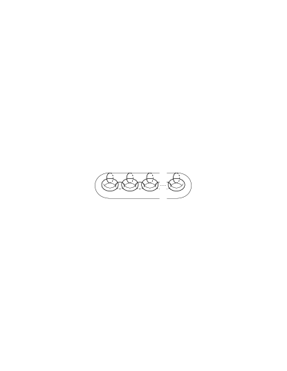
The (homeomorphism class of) the mapping torus $T_{g,f}$ depends only on the isotopy class of $f$. The orientation-preserving self-homeomorphisms of $\Sigma_{g}$ form a group under composition. This group, taken modulo isotopy, is called the mapping class group of $\Sigma_{g}$, and is denoted $\mathrm{MCG}(g)$. $\mathrm{MCG}(g)$ is generated by the Dehn twists about the $3g-1$ canonical curves shown in figure 1. Any mapping torus $T_{g,f}$ is thus described by a word in the Dehn twist generators of $\mathrm{MCG}(g)$.

Figure 1: A Dehn twist is a $2\pi$ rotation about a closed curve. The Dehn twists along the $3g-1$ curves illustrated here constitute a standard set of generators for the mapping class group of the genus $g$ surface.

2.2 The Witten-Reshetikhin-Turaev invariants

Recall that the genus is an invariant of surfaces because it assigns the same number to homeomorphic surfaces. One can also define invariants of $3$-manifolds, although none are as simple and powerful as the genus. In the 1990s, Witten, Reshetikhin, and Turaev discovered a family of $3$-manifold invariants arising from their work in Topological Quantum Field Theory. While these invariants can be defined for arbitrary $3$-manifolds, we only concern ourselves with the special case of mapping tori, where the definitions are relatively straightforward. Specifically, the Witten-Reshetikhin-Turaev (WRT) invariant of a mapping torus $T_{g,f}$ is equal to the trace of $f$ in a certain projective representation of the mapping class group $\mathrm{MCG}(g)$. Note that the WRT function is only a topological invariant up to a phase (see [3]). In general, the WRT invariant is parametrized by a quantum group, such as $\mathrm{SU}(N)_{k}$ or $\mathrm{SO}(N)_{k}$. Although some of our results apply more generally, we focus on the case of $\mathrm{SO}(3)_{3}$, sometimes called the Fibonacci model. In this case, the description of the representation is particularly simple, and can be understood with no background in quantum groups.

Figure 2: The dashed lines indicate a set of cuts that decomposes the surface into two three-punctured-spheres (“pants”). Dual to this is a trivalent graph called the “spine,” in red. The genus two and genus three cases are shown here.

Figure 3: The Fibonacci model’s fusion rules allow five labelings of the standard spine of the genus two surface. This means that the WRT representation of $\mathrm{MCG}(2)$ is five-dimensional.

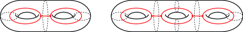
The Fibonacci representation is defined as follows. Any genus $g$ surface (for $g>1)$ can be cut into three-punctured spheres, resulting in a so-called pants decomposition. Dual to such a decomposition is a trivalent graph on the surface, called a spine. As illustrated in figure 2, the spine has one vertex for every pant in the decomposition. Whenever two pants meet at a puncture, the spine has an edge between the corresponding vertices. While a surface admits many spines (and corresponding pants decompositions), we call the one shown in figure 2 the standard spine. We label the edges of the standard spine by so-called anyon types, with fusion rules enforced at each vertex. For the Fibonacci model, there are only two anyon types: $0$ and $1$, and only one fusion rule: no vertex can have exactly two edges labeled $0$ incident on it. The case $g=2$ is pictured in figure 3. The formal span (over $\mathbb{C}$) of all such labelings associates a finite-dimensional vector space to the surface. Different spines yield different bases for this same space. We can move between these spines (and the corresponding bases) by means of two “moves,” the F-move:

$$\begin{array}[]{c}\includegraphics[width=56.37271pt]{fmove_noarrows2a.eps}\end{array}=\sum_{n}F^{ijm}_{kln}\begin{array}[]{c}\includegraphics[width=56.37271pt]{fmove_noarrows2b.eps}\end{array}$$

and the S-move:

$$\begin{array}[]{c}\includegraphics[width=56.37271pt]{smove_noarrows3a.eps}\end{array}=\sum_{k}S^{i}_{jk}\begin{array}[]{c}\includegraphics[width=56.37271pt]{smove_noarrows3b.eps}\end{array}$$

For the Fibonacci model $F_{abc}^{def}$ is as follows

with all other values equal to zero or one as dictated by the fusion rules. As one can calculate using the prescription described in [3], $S^{i}_{jk}$ is given in the Fibonacci model by

$$DS^{0}_{00} = 1$$

$$DS^{0}_{10}=DS^{0}_{01} = \frac{1+\sqrt{5}}{2}$$

$$DS^{0}_{11} = 1+\frac{1+\sqrt{5}}{2}e^{i4\pi/5}$$

$$DS^{1}_{11} = \sqrt{\frac{1+\sqrt{5}}{2}}\left(1-e^{i4\pi/5}\right)$$

with $D=\sqrt{1+\left(\frac{1+\sqrt{5}}{2}\right)^{2}}$ and all other values of $S^{i}_{jk}$ equal to zero by the fusion rules.

The space described above is the underlying vector space for the Fibonacci representation of $\mathrm{MCG}(g)$. We define this representation in the basis corresponding to the standard spine. Since the mapping class group is finitely-generated, it suffices to describe the images of the Dehn twist generators. Any such generator is a $2\pi$ twist along some canonical curve $c$ from figure 1. It is not hard to check that, by applying at most one F-move and one S-move, the standard spine can be adjusted so that $c$ is a cut in the corresponding pants decomposition. In this basis, the Dehn twist about $c$ induces a diagonal linear transformation. To each labeling of the spine corresponds a basis vector, and this basis vector obtains a phase determined by the label on the edge of the spine that intersects $c$. In the Fibonacci model, edges labeled 0 obtain a phase of 1, and edges labeled 1 obtain a phase of $e^{i3\pi/5}$. In the standard spine basis, the matrix corresponding to the Dehn twist about $c$ is thus simply a product of at most five matrices: at most two of the moves pictured above, followed by a diagonal matrix, followed by the inverse moves to return to the original basis. The WRT invariant of the mapping torus $T_{g,f}$ is now simply the trace of the Fibonacci representation, evaluated at $f$.

2.3 One Clean Qubit

In some proposed implementations of quantum computers, such as nuclear magnetic resonance (NMR) the most difficult task is initializing qubits into a pure state. In 1998, Knill and Laflamme proposed that exponential speedups over classical computation might be possible without pure state initialization. To mathematically investigate this possibility, they introduced the one clean qubit model [17]. In this model, one is given an initial state $\rho$ with $n$ qubits in the maximally mixed state, and one qubit in the pure state $\left|{0}\right\rangle$.

$$\rho=\left|{0}\right\rangle\left\langle{0}\right|\otimes\frac{\mathds{1}}{2^{n}}$$

One then applies any quantum circuit of $\mathrm{poly}(n)$ gates to this state, and measures the first qubit in the computational basis. Computational problems are solved by performing polynomially many such experiments, each starting with the initial state $\rho$, and recording the output statistics. The class of decision problems solvable with bounded probability of error using this procedure is called DQC1.

DQC1 contains several computational problems not known to be solvable in polynomial time on classical computers. Most fundamentally, given a description of a quantum circuit of $T$ gates implementing the unitary transformation $U$ on $n$ qubits, a one clean qubit computer can estimate the normalized trace $\frac{\mathrm{Tr}{U}}{2^{n}}$ to within $\pm\epsilon$ in time $O(T/\epsilon^{2})$ by means of the circuit shown in figure 4. Furthermore, this problem of estimating the trace of a quantum circuit is DQC1-hard [17, 24, 25]. Efficient one clean qubit algorithms have been discovered for estimating certain quadratically signed weight enumerators [18] and estimating certain Jones [25] and HOMFLY [16] polynomials. A version of the Jones polynomial problem is DQC1-complete [25], and has been demonstrated experimentally with NMR [22, 20]. A certain problem of approximating partition functions for quantum systems is also DQC1-hard [6].

In many ways, it is surprising that one clean qubit computers can do any nontrivial computations at all. If all $n+1$ qubits were maximally mixed, the resulting state would be invariant under all unitaries. Furthermore, DQC1 computations involve very little entanglement [7, 9, 8, 10, 11, 19]. Ambainis et al. give an impossibility proof against a certain natural approach to simulating standard quantum computers using one clean qubit computers, and on the other hand show that one clean qubit computers can efficiently simulate classical logarithmic depth (NC1) computations [4].

The DQC1 complexity class is robust against a variety of modifications to the computational model. The class of computational problems solvable in polynomial time with up to logarithmically many clean qubits is the same as that solvable in polynomial time with one clean qubit [25]. If the clean qubit is not pure, but has $1/\mathrm{poly}(n)$ polarization, the set of efficiently solvable problems also remains DQC1 [17]. As shown in appendix A, the one clean qudit model on $d$-dimensional qudits is equivalent in power to the one clean qubit model, for any constant $d$.

$$\begin{array}[]{lll}\lx@xy@svg{\hbox{\raise 0.0pt\hbox{\kern 0.0pt\hbox{\ignorespaces\ignorespaces\ignorespaces\hbox{\vtop{\kern 0.0pt\offinterlineskip\halign{\entry@#!@&&\entry@@#!@\cr&&&&\\&&&&\crcr}}}\ignorespaces{\hbox{\kern 0.0pt\raise 0.0pt\hbox{\hbox{\kern-47.389pt\raise-2.5pt\hbox{$\textstyle{\frac{1}{\sqrt{2}}(\left|{0}\right\rangle+\left|{1}\right\rangle)}$}}}}}{\hbox{\kern 10.00002pt\raise 0.0pt\hbox{\hbox{\kern-3.0pt\raise 0.0pt\hbox{\hbox{\kern 3.0pt\raise 0.0pt\hbox{$\textstyle{\ignorespaces\ignorespaces\ignorespaces\ignorespaces}$}}}}}}}\ignorespaces\ignorespaces\ignorespaces\ignorespaces{}{\hbox{\lx@xy@droprule}}\ignorespaces{}{\hbox{\lx@xy@droprule}}{\hbox{\lx@xy@droprule}}{\hbox{\kern 27.73685pt\raise 0.0pt\hbox{\hbox{\kern-3.27777pt\raise-2.47217pt\hbox{$\textstyle{\bullet}$}}}}}\ignorespaces\ignorespaces\ignorespaces\ignorespaces{}\ignorespaces{}{\hbox{\lx@xy@droprule}}{\hbox{\lx@xy@droprule}}\ignorespaces\ignorespaces\ignorespaces\ignorespaces{}\ignorespaces{}{\hbox{\lx@xy@droprule}}{\hbox{\lx@xy@droprule}}{\hbox{\kern 43.91814pt\raise 0.0pt\hbox{\hbox{\kern 0.0pt\raise 0.0pt\hbox{$\textstyle{\lx@xy@svgnested{\hbox{\raise 0.0pt\hbox{\kern 7.56252pt\hbox{{\hbox{\kern-7.56252pt\raise 0.0pt\hbox{\hbox{\kern 3.00003pt\raise-3.41666pt\hbox{$\textstyle{H}$}}}}}\ignorespaces\ignorespaces\ignorespaces\ignorespaces\ignorespaces{\hbox{\lx@xy@droprule}}\ignorespaces\ignorespaces\ignorespaces\ignorespaces\ignorespaces\ignorespaces{\hbox{\lx@xy@droprule}}\ignorespaces\ignorespaces\ignorespaces\ignorespaces\ignorespaces\ignorespaces{\hbox{\lx@xy@droprule}}\ignorespaces\ignorespaces\ignorespaces\ignorespaces\ignorespaces{\hbox{\lx@xy@droprule}}}}}}}$}}}}}\ignorespaces\ignorespaces\ignorespaces\ignorespaces{}{\hbox{\lx@xy@droprule}}\ignorespaces{}{\hbox{\lx@xy@droprule}}{\hbox{\kern 69.04318pt\raise 0.0pt\hbox{\hbox{\kern 0.0pt\raise 0.0pt\hbox{$\textstyle{\lx@xy@svgnested{\hbox{\raise 0.0pt\hbox{\kern 9.00009pt\hbox{{\hbox{\kern-9.00009pt\raise 0.0pt\hbox{\hbox{\kern 3.00003pt\raise 0.0pt\hbox{$\textstyle{\lx@xy@svgnested{\hbox{\raise 0.0pt\hbox{\kern 6.00006pt\hbox{{\hbox{\kern-11.00008pt\raise 0.0pt\hbox{\hbox{\kern 0.0pt\raise-11.00008pt\hbox{\cirbuild@}}}}}\ignorespaces\ignorespaces\ignorespaces\ignorespaces{\hbox{\lx@xy@drawline@}}{}{}}}}}}$}}}}}\ignorespaces\ignorespaces\ignorespaces\ignorespaces\ignorespaces{\hbox{\lx@xy@droprule}}\ignorespaces\ignorespaces\ignorespaces\ignorespaces\ignorespaces\ignorespaces{\hbox{\lx@xy@droprule}}\ignorespaces\ignorespaces\ignorespaces\ignorespaces\ignorespaces\ignorespaces{\hbox{\lx@xy@droprule}}\ignorespaces\ignorespaces\ignorespaces\ignorespaces\ignorespaces{\hbox{\lx@xy@droprule}}}}}}}$}}}}}\ignorespaces\ignorespaces\ignorespaces\ignorespaces{}{\hbox{\lx@xy@droprule}}\ignorespaces{}{\hbox{\lx@xy@droprule}}{\hbox{\lx@xy@droprule}}{\hbox{\kern 0.0pt\raise-20.41663pt\hbox{\hbox{\kern-10.90094pt\raise-2.25555pt\hbox{$\textstyle{\frac{\mathds{1}}{2^{n}}}$}}}}}{\hbox{\kern 10.00002pt\raise-20.41663pt\hbox{\hbox{\kern-5.5pt\raise 0.0pt\hbox{\hbox{\kern 3.0pt\raise 0.0pt\hbox{$\textstyle{{/}\ignorespaces\ignorespaces\ignorespaces\ignorespaces}$}}}}}}}\ignorespaces\ignorespaces\ignorespaces{{{}{}}}\ignorespaces{}{\hbox{\lx@xy@droprule}}\ignorespaces{}{\hbox{\lx@xy@droprule}}{\hbox{\lx@xy@droprule}}{\hbox{\kern 20.00003pt\raise-20.41663pt\hbox{\hbox{\kern 0.0pt\raise 0.0pt\hbox{$\textstyle{\lx@xy@svgnested{\hbox{\raise 0.0pt\hbox{\kern 6.95905pt\hbox{{\hbox{\kern-6.95905pt\raise 0.0pt\hbox{\hbox{\kern 3.00003pt\raise-3.41666pt\hbox{$\textstyle{U}$}}}}}\ignorespaces\ignorespaces\ignorespaces\ignorespaces\ignorespaces{\hbox{\lx@xy@droprule}}\ignorespaces\ignorespaces\ignorespaces\ignorespaces\ignorespaces\ignorespaces{\hbox{\lx@xy@droprule}}\ignorespaces\ignorespaces\ignorespaces\ignorespaces\ignorespaces\ignorespaces{\hbox{\lx@xy@droprule}}\ignorespaces\ignorespaces\ignorespaces\ignorespaces\ignorespaces{\hbox{\lx@xy@droprule}}}}}}}$}}}}}\ignorespaces\ignorespaces\ignorespaces{{{}{}}}\ignorespaces{}{\hbox{\lx@xy@droprule}}\ignorespaces{}{\hbox{\lx@xy@droprule}}{\hbox{\lx@xy@droprule}}{\hbox{\kern 51.48065pt\raise-20.41663pt\hbox{\hbox{\kern-5.5pt\raise 0.0pt\hbox{\hbox{\kern 3.0pt\raise 0.0pt\hbox{$\textstyle{{/}\ignorespaces\ignorespaces\ignorespaces\ignorespaces}$}}}}}}}\ignorespaces\ignorespaces\ignorespaces{{{}{}}}\ignorespaces{}{\hbox{\lx@xy@droprule}}\ignorespaces{}{\hbox{\lx@xy@droprule}}{\hbox{\lx@xy@droprule}}{\hbox{\kern 78.04327pt\raise-20.41663pt\hbox{\hbox{\kern-3.0pt\raise 0.0pt\hbox{\hbox{\kern 3.0pt\raise 0.0pt\hbox{$\textstyle{\ignorespaces\ignorespaces\ignorespaces\ignorespaces}$}}}}}}}\ignorespaces\ignorespaces\ignorespaces{{{}{}}}\ignorespaces{}{\hbox{\lx@xy@droprule}}\ignorespaces{}{\hbox{\lx@xy@droprule}}{\hbox{\lx@xy@droprule}}\ignorespaces}}}}\ignorespaces&&p_{0}=\frac{1}{2}+\frac{\mathrm{Re}(\mathrm{Tr}[U])}{2^{n}}\end{array} \textstyle{\frac{1}{\sqrt{2}}(\left|{0}\right\rangle+\left|{1}\right\rangle)} \textstyle{\bullet} \textstyle{H} \textstyle{\frac{\mathds{1}}{2^{n}}} \textstyle{{/}\ignorespaces\ignorespaces\ignorespaces\ignorespaces} \textstyle{U} \textstyle{{/}\ignorespaces\ignorespaces\ignorespaces\ignorespaces} \textstyle{\frac{1}{\sqrt{2}}(\left|{0}\right\rangle+\left|{1}\right\rangle)} \textstyle{\bullet} \textstyle{H} \textstyle{\frac{\mathds{1}}{2^{n}}} \textstyle{{/}\ignorespaces\ignorespaces\ignorespaces\ignorespaces} \textstyle{U} \textstyle{{/}\ignorespaces\ignorespaces\ignorespaces\ignorespaces}$$

Figure 4: By repeating this one clean qubit computation, and recording the fraction of $0$ outcomes, one estimates the real part of $\mathrm{Tr}[U]/2^{n}$. Similarly, by initializing the clean qubit to $\frac{1}{\sqrt{2}}(\left|{0}\right\rangle-i\left|{1}\right\rangle)$, one obtains $p_{0}=\frac{1}{2}+\frac{\mathrm{Im}(\mathrm{Tr}[U])}{2^{n}}$.

3 Algorithm

In this section we construct an efficient one clean qubit algorithm for approximating the Fibonacci WRT invariant of a mapping torus. Generalizing to other tensor categories such as $\mathrm{SU}(N)_{k}$ and $\mathrm{SO}(N)_{k}$ is straightforward. The main idea of the algorithm is, given a word $w$ in the Dehn twist generators of $\mathrm{MCG}(g)$, to find a quantum circuit of $\mathrm{poly}(w,g)$ gates on $\mathrm{poly}(g)$ qubits whose trace is equal to the WRT invariant of the $3$-manifold $T_{g,w}$. This trace can then be approximated by means of the circuit in figure 4. For this purpose, we encode the allowed labelings of a spine of $\Sigma_{g}$ into qubits, and then construct a quantum circuit implementing the Fibonacci representation of $\mathrm{MCG}(g)$ on this encoding. The most obvious encoding would be to directly assign one qubit to store the particle type for each edge of the spine. However, a one clean qubit computer yields the normalized trace over all $2^{n}$ bitstrings, of which only an exponentially small fraction represent valid spine labelings in this encoding.

We instead construct a many-to-one map $\varphi:\{0,1\}^{\beta(3g-3)}\to\{\textrm{valid labelings}\}$ with $\beta=O(\log|g|)$ such that the preimage of each spine-labeling consists of approximately the same number of bitstrings. That is, $|\varphi^{-1}(x)|$ is approximately independent of $x$. Thus, the normalized trace of the Fibonacci representation of $w\in\mathrm{MCG}(g)$ acting on the $\varphi$-encoded labelings of the spine of $\Sigma_{g}$ is approximately equal to $\mathrm{WRT}(T_{g,w})$. We construct $\varphi$ following a method introduced in [16]. We assign a register of $\beta=O(\log|g|)$ qubits to each edge of the spine. The bitstring contained in register $i$ is interpreted as an integer $0\leq x_{i}\leq 2^{\beta}-1$. We then assign a threshold $T_{i}$ so that $x_{i}\leq T_{i}$ encodes a zero label on edge $i$, and $x_{i}>T_{i}$ encodes a one label. By carefully choosing the thresholds $T_{1},\ldots,T_{3g-3}$ we ensure that $|\varphi^{-1}(x)|$ is approximately independent of $x$.

Figure 5: We number the edges of the standard spine from left to right, with ambiguities resolved by ordering from top to bottom.

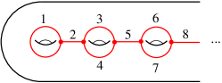
Number the edges of the spine from one to $3g-3$, left to right and top to bottom, as illustrated in figure 5. Let $s_{1},\ldots,s_{3g-3}\in\{0,1\}^{3g-3}$ be the labels of these edges. The uniform probability distribution over all fusion-consistent labelings of the spine induces a probability distribution $p_{g}(s_{1}\ldots,s_{3g-3})$ over $\{0,1\}^{3g-3}$, with zero probability for strings that violate fusion rules, and uniform probability for the rest. For the genus-$g$ standard spine, we define $p_{g}(s_{i}|s_{1},\ldots,s_{i-1})$ to be the conditional probability that label $i$ takes the value $s_{i}$ given that labels 1 through $i-1$ take the values $s_{1},\ldots,s_{i-1}$. For a register representing a label $s_{i}$ we choose the threshold dependent on the values of $s_{1},\ldots,s_{i-1}$ according to

$$T_{i}(g;s_{1},\ldots,s_{i-1})=\left\lceil 2^{\beta}p_{g}(0|s_{1},\ldots,s_{i-1})\right\rfloor.$$ (1)

One can see that this choice ensures that a uniformly selected assignment of bitstrings to the registers yields a uniform distribution over fusion-consistent labelings, up to the errors induced by rounding. Hence, $|\varphi^{-1}(x)|$ is approximately independent of $x$. More precisely, let

$$\tilde{p}_{g}(0|s_{1},\ldots,s_{i-1}) = T_{i}(g;s_{1},\ldots,s_{i-1})/2^{\beta}$$

$$\tilde{p}_{g}(1|s_{1},\ldots,s_{i-1}) = 1-\tilde{p}_{g}(0|s_{1},\ldots,s_{i-1})$$

Thus,

$$|\varphi^{-1}(s_{1},\ldots,s_{3g-3})| = 2^{\beta(3g-3)}\tilde{p}_{g}(s_{3g-3}|s_{1},\ldots,s_{3g-4})\times\tilde{p}_{g}(s_{3g-4}|s_{1},\ldots,s_{3g-5})\times\ldots\times p(s_{1})$$

$$= 2^{\beta(3g-3)}\left(p_{g}(s_{3g-3}|s_{1},\ldots,s_{3g-4})\pm O(2^{-\beta})\right)\times\ldots\times\left(p_{g}(s_{1})\pm O(2^{-\beta})\right)$$

$$= p_{g}(s_{1},\ldots,s_{3g-3})\pm O(g2^{-\beta}).$$

Thus it suffices to choose $\beta=O(\log g)$. Furthermore, by the locality of the fusion rules, $p_{g}(s_{i}|s_{1},\ldots,s_{i-1})$ is always independent of $s_{1},\ldots,s_{i-3}$. We may thus write

$$p_{g}(s_{i}|s_{1},\ldots,s_{i-1}) = p_{g}(s_{i},s_{i-1},s_{i-2};i)$$

$$T_{i}(g;s_{1},\ldots,s_{i-1}) = T_{i}(g;s_{i},s_{i-1},s_{i-2}).$$ (2)

$$\begin{array}[]{rl}\begin{array}[]{c}\includegraphics[width=73.7146pt]{thicklocal1.eps}\end{array}&\textrm{acts on $a,b,c,d$}\\ \begin{array}[]{c}\includegraphics[width=73.7146pt]{thicklocal2.eps}\end{array}&\textrm{acts on $a$}\\ \begin{array}[]{c}\includegraphics[width=108.405pt]{thicklocal3.eps}\end{array}&\textrm{acts on $a,b,c,d,e$ }\end{array}$$

Figure 6: The Fibonacci representation of a Dehn twist (shown as a dashed line) from the standard generating set is a unitary transformation acting on at most five spine labels.

As illustrated in figure 6, the Fibonacci representation of a Dehn twist from the standard generating set is a unitary transformation acting on at most five spine labels. Because the encoding $\varphi$ is many-to-one, the unitary transformation on these spine labels does not uniquely define a unitary operation on the bitstrings encoding them. We say that a pair of spine-labelings is connected if the Fibonacci representation of a Dehn twist from the standard set of generators has a nonzero matrix element between them. By choosing a bijection $b_{x,y}$ between the encodings of each pair of connected spin-labelings we define a unitary transformation on the encodings: if the matrix element between labeling $x$ and $y$ is $\rho_{x,y}$ then,

$$U_{i,j}=\left\{\begin{array}[]{ll}\rho_{x,y}&\textrm{if $\varphi(i)=x$, $\varphi(j)=y$, and $b_{x,y}(i)=j$}\\ 0&\textrm{otherwise}\end{array}\right.$$ (3)

is a corresponding unitary representation on the encodings. Our choice of bijections does not matter. We may for concreteness match bitstrings by lexicographic ordering. One can verify that $U$ is a direct sum of many copies of the Fibonacci representation $\rho$. (The rounding involved in (1) introduces a minor technical complication, whose resolution may be found in [16].)

For any of the standard Dehn twist generators, $U_{i,j}$ acts on at most $5\beta$ qubits, which encode the spine-labels on which $\rho$ acts. The matrix elements by which $U$ acts on these qubits depends on the corresponding thresholds. By (2), these depend on at most two additional registers of qubits, which encode the two spine labels to the left of those being acted upon. Thus, for any of the standard Dehn twist generators, $U_{i,j}$ is a controlled unitary acting on at most $5\beta$ target qubits and $2\beta$ control qubits. Recalling that $\beta=O(\log|g|)$, we can apply the standard construction from section 4.5 of [21] to implement this unitary transformation with $\textrm{poly}(|g|)$ quantum gates, provided each matrix element of $U_{i,j}$ can be computed efficiently. By (3), one sees that the only potentially difficult part of computing the matrix elements of 3 is the computation of the thresholds. An efficient classical algorithm for this task is given in appendix C.

4 Hardness

In this section we prove that the problem of estimating the normalized WRT Fibonacci invariant of a mapping torus, given by a polynomial-length word in the standard Dehn twist generators of the mapping class group, to within $\pm\epsilon$ is DQC1-hard for $\epsilon<1/3900$. Generalizing our hardness proof beyond the Fibonacci model seems less straightforward than generalizing our algorithm. However, we consider it likely to be possible. Extending hardness to larger values of $\epsilon$ we leave as an open problem. To prove hardness, we reduce from the problem of estimating the absolute value of the normalized trace of a quantum circuit. A proof of the hardness of absolute trace estimation is given in appendix B. We thus require an efficient procedure that, given a description of a quantum circuit for implementing a unitary $U$, outputs a description of a mapping torus (i.e., a word in the Dehn twist generators) whose WRT invariant is close to the trace of $U$. It turns out to be convenient to suppose that $U$ is a quantum circuit acting on a collection of 5-dimensional qudits (“qupents”). As shown in appendix A, this makes no difference: the one-clean-qubit model is equivalent to the one-clean-qupent model.

Let $U$ be a quantum circuit of $G$ gates acting on $n$ qupents arranged in a line. Without loss of generality, we may assume that each gate acts either on a single qupent or a pair of neighboring qupents. To prove hardness, we first define a many-to-one encoding $\psi:S_{3n}\to\{0,1,2,3,4\}^{n}$, where $S_{3n}$ is the set of fusion-consistent labelings of the standard spine of the surface of genus $3n$. We divide the genus-$3n$ surface into $n$ segments, each having three handles. The number of fusion-consistent labelings for a genus-three segment with two punctures depends on the labels on the incoming and outgoing edges, as shown below.

In all cases, the number of fusion-consistent labelings is a multiple of five. Thus, in every case a qupent can be encoded in the space of labelings, together with a “gauge” qudit, whose value we ignore, which has dimension 3, 4, or 7, depending on the labels of the incoming edges. Thus the size $|\psi^{-1}(z)|$ of the preimage of any $z\in\{0,1,2,3,4\}^{n}$ is exactly independent of $z$. Given any unitary $U$ acting on $n$ qupents, there corresponds a unitary acting on the span of $S_{3n}$ which acts as $U$ on the encoded qupents, and as the identity on the gauge qudits. We call this the $\psi$-encoding of $U$.

As shown in [14], the Fibonacci representation of the mapping class group of the genus $g>1$ surface is dense in the corresponding unitary group, modulo phase. Thus, given any unitary operation on $n$ qupents, we can find a sequence of Dehn twists which approximates its $\psi$-encoding arbitrarily closely. The trace of the $\psi$-encoding is thus equal to the trace of the original quantum circuit, up to a phase. The remaining question is whether this reduction can be done efficiently.

Cutting the genus-$3n$ surface into $n$ equal segments yields $n-2$ genus-3 doubly-punctured surfaces, and two genus-3 singly-punctured surfaces, as shown below.

One can pants-decompose a punctured surface, thereby associating the surface to a spine. The spine has one “external”edge for each puncture, which attaches to the rest of the spine at only one vertex. Upon labeling the spine, we can associate the label of any external edge with the corresponding puncture. The Fibonacci representation may then be extended to the label-preserving mapping class group of the punctured surface. This group includes all the standard Dehn twists, together with braiding of punctures with the other punctures of the same label. In the Fibonacci representation, braiding of zero-labeled punctures has no effect, thus a zero-labeled puncture is equivalent to the absence of a puncture.

Theorem 6.2 of [14] states that for any fixed labels on the punctures, the Fibonacci representation of the label-preserving mapping class group of the $r$-punctured genus-$g$ surface is dense in the corresponding unitary group modulo phase, provided $g+r>1$. Thus, given any one-qupent gate, the Solovay-Kitaev theorem [21] efficiently yields a sequence of Dehn twists and braid moves on the corresponding genus-3 singly-punctured or doubly-punctured surface, whose Fibonacci representation approximates the $\psi$-encoded gate arbitrarily closely. Similarly, one efficiently approximates two-qupent gates by moves on genus-6 surfaces with one or two punctures.

We must modify the above construction so as not to use any braiding of punctures. On the leftmost or rightmost qupents there is no problem; the corresponding surfaces have only one puncture, and therefore theorem 6.2 implies density without using any braiding moves. Similarly, on any of the central surfaces, theorem 6.2 implies density without using any braiding moves if at least one of the punctures has a zero label. We can ensure this prior to the application of any given gate by adapting the “inchworm” technique from [25], as described in appendix D. In this method, we bring a pair of zero labels adjacent to the target segment, then implement the desired gate there, and carry the zeros to the segment where the next gate is to be implemented. At the end, we return these zeroes to their original location among the leftmost six handles. As discussed in appendix D, the inchworm construction entails some overhead in $\epsilon$, which gives rise to the value $1/3900$.

In the above construction, we need density on two-punctured segments in which one puncture is guaranteed to be labeled zero, and the other puncture has unknown label. Theorem 6.2 of [14] implies density separately in the subspace in which the other label is zero and in which the other label is one. Because these subspaces have different dimension (20 and 15, respectively) we may apply the decoupling lemma from [1], which shows that a sequence of Dehn twists can be found to approximate arbitrary pairs of independent unitaries on these two subspaces, as desired.

5 Analogy with Jones polynomials

In this paper we have shown that estimating the Turaev-Viro invariant of a mapping torus in the Fibonacci model is DQC1-complete. In [3], it was shown that estimating the Turaev-Viro invariant of a general 3-manifold presented as a Heegaard splitting is BQP-complete. Similarly, estimating the Jones polynomial of the trace closure of a braid is DQC1-complete [25, 16], while estimating the Jones polynomial of the plat closure of a braid is BQP-complete [2, 1, 29, 13, 12]. This suggests a relationship between trace closures and mapping tori on one hand, and between plat closures and Heegaard splittings on the other. Indeed, such a relationship can be understood in the framework of axiomatic topological quantum field theory, and suggests further generalizations to, for instance, topological invariants of higher dimensional manifolds.

Figure 7: The problems of estimating the Jones polynomial of the plat closure of a braid and the Turaev-Viro invariant of a Heegaard splitting (left) are BQP-complete. The problems of estimating the Jones polynomial of the trace closure of a braid and the Turaev-Viro invariant of a mapping torus (right) are DQC1-complete. These situations are fundamentally analogous, as discussed in section 5. We stress that the manifold figures are illustrations of the topological ideas behind this analogy, and are not correct two-dimensional projections of the manifolds themselves. In particular, after gluing, the two manifolds shown do not in reality have any boundaries.

Figure 8: $M$ can be viewed as a two-manifold with two boundaries: a circle and a pair of circles. The TQFT associates a Hilbert space $T(C_{2})$ to the pair of circles, a Hilbert space $T(C_{1})$ to the circle, and a linear transformation $T(M):T(C_{2})\to T(C_{1})$ to $M$. Similarly, $T(N)$ is a linear transformation from $T(C_{1})$ to itself. If we glue together $M$ and $N$ along the circle as shown, we obtain a manifold $MN$ with boundaries $C_{2}$ and $C_{1}$. The corresponding linear transformation is $T(NM)=T(N)\circ T(M)$.

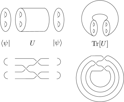
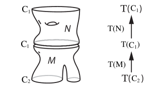
A topological quantum field theory can be axiomatized as a functor $T$ from the category of cobordisms between $n$-manifolds to the category of linear transformations between vector spaces [5, 28]. That is, to each $n$-manifold the TQFT associates a vector space, and to any $(n+1)$-manifold whose boundary is the union of two disjoint $n$-manifolds the TQFT associates a linear transformation between the two associated vector spaces. The functorial property means that gluing together two cobordisms and then applying $T$ yields the same linear transformation that is obtained by applying $T$ to each of the two cobordisms and then composing the resulting linear transformations; see figure 8. A TQFT maps the empty $n$-manifold to the base field, which for the examples we consider is always $\mathbb{C}$. Hence, for $M$ a manifold whose boundary $\partial M$ has a single connected component, $T(M)$ is a map either from $\mathbb{C}$ to the vector space $T(\partial M)$, that is, a vector in $T(\partial M)$, or a map from $T(\partial M)$ to $\mathbb{C}$, that is, a dual vector. The choice between these two possibilities is determined by the orientation of the cobordism.

Recall that the genus-$g$ handlebody is the $3$-manifold whose boundary is the genus-$g$ surface $\Sigma_{g}$. For example, the genus-1 handlebody is simply the solid donut. After assigning an orientation, we may think of a handlebody as a cobordism from the empty manifold to $\Sigma_{g}$, or as a cobordism from $\Sigma_{g}$ to the empty manifold. Hence, in the TQFT framework, genus-$g$ handlebodies are associated to vectors or dual vectors. We denote these as $\left|{\psi_{g}}\right\rangle$ and $\left\langle{\psi_{g}}\right|$, respectively. These vectors live in the Hilbert space which the TQFT associates to $\Sigma_{g}$. In the case of the Fibonacci model, this is precisely the vector space defined in Section 2.2.

In the Fibonacci model, a cobordism from a surface to itself is mapped to a unitary linear transformation $U$ on the associated Hilbert space. If the surface is $\Sigma_{g}$, then we may “cap” the cobordism with handlebodies on both ends. The resulting $3$-manifold has no boundary, and thus corresponds to a linear map from $\mathbb{C}$ to itself, i.e., a complex number. In this case, this number is the matrix element $\left\langle{\psi_{g}}\right|U\left|{\psi_{g}}\right\rangle$, as illustrated in figure 7. The problem of estimating a matrix element of the unitary transformation induced by a quantum circuit is BQP-complete, and this fact underlies the BQP-completeness proof for the Turaev-Viro invariant of Heegaard splittings in [3]. Instead of “capping” the two ends of the cobordism with handlebodies, we could have simply glued the two ends together, resulting in a mapping torus. This is again a $3$-manifold without boundary, which thus also corresponds to a complex number. In a TQFT, gluing the two ends of a cobordism corresponds to contracting the two indices of the linear transformation. In other words, instead of a single matrix entry, we now obtain the trace of $U$. Finding the trace of the unitary transformation induced by a quantum circuit is DQC1-complete, and this fact underlies the DQC1-completeness proof for the Turaev-Viro invariant of mapping tori given in this paper.

The situation regarding Jones polynomials is directly analogous. A TQFT gives us a unitary representation of the braid group. Gluing the two ends of a braid together (i.e., taking the trace closure), as illustrated on the righthand side of figure 7, corresponds to taking the trace of the unitary and yields a DQC1-complete problem. Caps correspond to vectors and dual vectors depending on orientation, hence capping a braid (taking the plat closure, as illustrated on the lefthand side of figure 7) yields a matrix element of the associated unitary transformation, and corresponds to a BQP-complete problem. The analogy can be tightened further by noting that the braid group $B_{n}$ is simply the mapping class group of the surface of genus zero and $n+1$ punctures (that is, the $n$-punctured disk), whereas in the case of 3-manifold invariants we consider the mapping class group of the genus-$g$ surface with no punctures. On the other hand, it is worth bearing in mind that the notion of equivalence captured by the Jones polynomial is ambient isotopy, in contrast to the Turaev-Viro and WRT invariants, which capture homeomorphism.

The analogy presented here naturally suggests an extension of BQP-completeness and DQC1-completeness results to $n$-manifold invariants arising from TQFTs at higher $n$. More generally, one could attempt to isolate a property of pairs, consisting of a group $G$ and one of its representations $U$, such that estimating matrix entries of $U$ is BQP-complete while estimating the trace of $U$ is DQC1-complete. Perhaps one could find a general theorem encompassing many such results. We leave this as an open problem.

6 Acknowledgments

We thank Robert König, Ben Reichardt and Edgar Bering for useful discussions and some diagrams. S.J. acknowledges support from the Sherman Fairchild Foundation and NSF grant PHY-0803371. G.A. acknowledges support from NSERC, MITACS and ARO.

Appendix A Equivalence Between One Clean Qudit Models

Given a quantum circuit on $a$-dimensional qudits we wish to construct a quantum circuit on $b$-dimensional qudits that has the same trace. If $b=ca$ for some integer $c$ then this is easy. We just consider each $b$-dimensional qudit to be an $a$-dimensional qudit plus a $c$-dimensional “gauge” qudit that we ignore. Similarly, if $b^{d}=ca$ for some integers $d,c$ then we can treat $d$-tuples of $b$-dimensional qubits as an $a$-dimensional qudit plus a $c$-dimensional gauge qudit. For these encodings, the encoded circuit is easy to construct gate by gate. Given a gate acting on $n$ $a$-dimensional qudits, we can write down a unitary acting on $dn$ $b$-dimensional qudits equal to the original gate tensored with the $c$-dimensional identity on the gauge system. This $dn$-dimensional gate can be exactly decomposed into a product of $O(b^{2dn})$ 2-qudit gates using the standard construction from section 4.5 of [21]. Because $d$ and $n$ are constants, this is sufficiently efficient. The normalized trace of the encoded circuit is exactly equal to the normalized trace of the original circuit.

The harder case is when there do not exist integers $c$ and $d$ such that $b^{d}=ca$. In this case we find $c,d\in\mathbb{Z}$ such that $b^{d}\simeq ca$. Specifically, suppose we achieve

$$\frac{ca}{b^{d}}=1-\delta$$ (4)

for some $\delta\ll 1$. Then we can encode one $a$-dimensional qudit plus a $c$-dimensional gauge qudit into $d$ $b$-dimensional qudits with a few (namely $\delta b^{d}$) noncoding states left over. We can define our encoded gates to act as the identity on these noncoding states. If we make sure the noncoding states are a small fraction of all $b^{dn}$ states, the normalized trace of the encoded circuit will approximately match the normalized trace of the original circuit.

Let $U_{a}$ be the original unitary acting on $n$ $a$-dimensional qudits and let $U_{b}$ be the unitary acting on $dn$ $b$-dimensional qudits, in which we encode $U_{a}$ as described above. Then, $U_{b}$ acts on $b^{dn}$ states, of which $(ca)^{n}$ encode states of the original circuit,

$$\frac{\mathrm{Tr}[U_{b}]}{b^{dn}}=\frac{c^{n}\mathrm{Tr}[U_{a}]+(b^{dn}-(ca)^{n})}{b^{dn}}.$$

The magnitude of the discrepancy $\Delta$ between the normalized traces of $U_{b}$ and $U_{a}$ is thus

$$\Delta = \left|\frac{c^{n}\mathrm{Tr}[U_{a}]+(b^{dn}-(ca)^{n})}{b^{dn}}-\frac{\mathrm{Tr}[U_{a}]}{a^{n}}\right|$$

$$= \left|\left(\left(\frac{ca}{b^{d}}\right)^{n}-1\right)\frac{\mathrm{Tr}[U_{a}]}{a^{n}}+1-\left(\frac{ca}{b^{d}}\right)^{n}\right|$$

$$\leq \left|\left(\frac{ca}{b^{d}}\right)^{n}-1\right|\cdot\left|\frac{\mathrm{Tr}[U_{a}]}{a^{n}}\right|+\left|1-\left(\frac{ca}{b^{d}}\right)^{n}\right|$$

$$\leq \left|\left(\frac{ca}{b^{d}}\right)^{n}-1\right|+\left|1-\left(\frac{ca}{b^{d}}\right)^{n}\right|$$

$$= 2\left|(1-\delta)^{n}-1\right|.$$

Thus if

$$\delta=\frac{\epsilon}{n}$$ (5)

we have, for small $\epsilon$,

$$\lim_{n\to\infty}\Delta=2\left|e^{-\epsilon}-1\right|\simeq 2\epsilon.$$ (6)

Comparing (4), (5), (6), we see that in the limit of large $n$ and small $\epsilon$, in order to achieve error upper bounded by $\Delta$ it suffices to obtain

$$\frac{b^{d}-ca}{b^{d}}\leq\frac{\Delta}{2n}.$$

For given $b,d,a$ there always exists an integer $c$ such that $b^{d}-c\leq a$. So we just need to choose $d$ sufficiently large that

$$\frac{a}{b^{d}}\leq\frac{\Delta}{2n}.$$

Equivalently,

$$d\geq\log_{b}\left(\frac{2na}{\Delta}\right).$$

A $k$-qudit gate from $U_{a}$ thus gets encoded as a $dk$-qudit gate in $U_{b}$. This encoded gate acts on a $b^{dk}$-dimensional space. We have just shown that it suffices to choose $d=\log_{b}\left(\frac{2na}{\Delta}\right)$. Thus the encoded $k$-qudit gate acts on a $\left(\frac{2na}{\Delta}\right)^{k}$-dimensional space. Using the construction from section 4.5 of [21], we can implement an arbitrary $D$-dimensional unitary exactly with $O(D^{2})$ 2-qudit gates. Thus each $k$-qudit gate in $U_{a}$ gets encoded by $O\left(\left(\frac{2na}{\Delta}\right)^{2k}\right)$ elementary gates in $U_{b}$. By gate universality, we can assume $k\leq 2$, so our encoding has an overhead quartic in $n$ and $1/\Delta$. This is perhaps not very efficient, but is nevertheless polynomial, and thus suffices to prove the equivalence of DQC1 defined with qudits of any constant dimension.

Appendix B Estimating the Absolute Trace is DQC1-hard

In this section we slightly adapt the proof from [24] to show that estimating the absolute value of the trace of a quantum circuit to within $\pm 1/24$ is a DQC1-complete problem. Consider an arbitrary DQC1 computation. We start with the state $\left|{0}\right\rangle\left\langle{0}\right|\otimes\frac{\mathds{1}}{2^{n}}$, apply an arbitrary quantum circuit $U$, and then measure the first qubit in the $\left|{0}\right\rangle,\left|{1}\right\rangle$ basis. Changing the initial state of the pure qubit, or changing the measurement basis does not add generality, as these changes can be subsumed into $U$. The probability of measurement outcome $\left|{0}\right\rangle$ is

$$p_{0}=\mathrm{Tr}\left[(\left|{0}\right\rangle\left\langle{0}\right|\otimes\mathds{1})U(\left|{0}\right\rangle\left\langle{0}\right|\otimes\mathds{1}/2^{n})U^{\dagger}\right].$$ (7)

Let $U^{\prime}$ be the unitary implemented by the following quantum circuit on $n+2$ qubits.

$$U^{\prime}=\begin{array}[]{l}\lx@xy@svg{\hbox{\raise 0.0pt\hbox{\kern 0.0pt\hbox{\ignorespaces\ignorespaces\ignorespaces\hbox{\vtop{\kern 0.0pt\offinterlineskip\halign{\entry@#!@&&\entry@@#!@\cr&&&&&&&\\&&&&&&&\\&&&&&&&\\&&&&&&&\crcr}}}\ignorespaces{\hbox{\kern 0.0pt\raise 0.0pt\hbox{\hbox{\kern-3.0pt\raise 0.0pt\hbox{\hbox{\kern 3.0pt\raise 0.0pt\hbox{$\textstyle{}$}}}}}}}{\hbox{\kern 10.00002pt\raise 0.0pt\hbox{\hbox{\kern-3.0pt\raise 0.0pt\hbox{\hbox{\kern 3.0pt\raise 0.0pt\hbox{$\textstyle{\ignorespaces\ignorespaces\ignorespaces\ignorespaces}$}}}}}}}\ignorespaces\ignorespaces\ignorespaces\ignorespaces{}{\hbox{\lx@xy@droprule}}\ignorespaces{}{\hbox{\lx@xy@droprule}}{\hbox{\lx@xy@droprule}}{\hbox{\kern 20.00003pt\raise 0.0pt\hbox{\hbox{\kern 5.0pt\raise-4.38889pt\hbox{$\textstyle{\hphantom{U^{\dagger}}}$}}}}}\ignorespaces\ignorespaces\ignorespaces\ignorespaces{}{\hbox{\lx@xy@droprule}}\ignorespaces{}{\hbox{\lx@xy@droprule}}{\hbox{\lx@xy@droprule}}\ignorespaces\ignorespaces{\hbox{\kern 25.00003pt\raise-12.38884pt\hbox{\hbox{\kern 0.0pt\raise-4.38889pt\hbox{$\textstyle{U^{\dagger}}$}}}}}\ignorespaces\ignorespaces\ignorespaces\ignorespaces\ignorespaces{\hbox{\lx@xy@droprule}}\ignorespaces\ignorespaces\ignorespaces\ignorespaces\ignorespaces{\hbox{\lx@xy@droprule}}\ignorespaces\ignorespaces\ignorespaces\ignorespaces\ignorespaces{\hbox{\lx@xy@droprule}}\ignorespaces\ignorespaces\ignorespaces\ignorespaces\ignorespaces{\hbox{\lx@xy@droprule}}{\hbox{\kern 55.1347pt\raise 0.0pt\hbox{\hbox{\kern-3.27777pt\raise-2.47217pt\hbox{$\textstyle{\bullet}$}}}}}\ignorespaces\ignorespaces\ignorespaces\ignorespaces{}\ignorespaces{}{\hbox{\lx@xy@droprule}}{\hbox{\lx@xy@droprule}}\ignorespaces\ignorespaces\ignorespaces\ignorespaces{}\ignorespaces{}{\hbox{\lx@xy@droprule}}{\hbox{\lx@xy@droprule}}{\hbox{\kern 68.30692pt\raise 0.0pt\hbox{\hbox{\kern 5.0pt\raise-3.41666pt\hbox{$\textstyle{\hphantom{U}}$}}}}}\ignorespaces\ignorespaces\ignorespaces\ignorespaces{}{\hbox{\lx@xy@droprule}}\ignorespaces{}{\hbox{\lx@xy@droprule}}\ignorespaces\ignorespaces{\hbox{\kern 73.30692pt\raise-12.38882pt\hbox{\hbox{\kern 0.0pt\raise-3.41666pt\hbox{$\textstyle{U}$}}}}}\ignorespaces\ignorespaces\ignorespaces\ignorespaces\ignorespaces{\hbox{\lx@xy@droprule}}\ignorespaces\ignorespaces\ignorespaces\ignorespaces\ignorespaces{\hbox{\lx@xy@droprule}}\ignorespaces\ignorespaces\ignorespaces\ignorespaces\ignorespaces{\hbox{\lx@xy@droprule}}\ignorespaces\ignorespaces\ignorespaces\ignorespaces\ignorespaces{\hbox{\lx@xy@droprule}}{\hbox{\kern 100.9527pt\raise 0.0pt\hbox{\hbox{\kern-3.27777pt\raise-2.47217pt\hbox{$\textstyle{\bullet}$}}}}}\ignorespaces\ignorespaces\ignorespaces\ignorespaces{}\ignorespaces{}{\hbox{\lx@xy@droprule}}{\hbox{\lx@xy@droprule}}\ignorespaces\ignorespaces\ignorespaces\ignorespaces{}\ignorespaces{}{\hbox{\lx@xy@droprule}}{\hbox{\lx@xy@droprule}}{\hbox{\kern 114.12491pt\raise 0.0pt\hbox{\hbox{\kern-3.0pt\raise 0.0pt\hbox{\hbox{\kern 3.0pt\raise 0.0pt\hbox{$\textstyle{\ignorespaces\ignorespaces\ignorespaces\ignorespaces}$}}}}}}}\ignorespaces\ignorespaces\ignorespaces\ignorespaces{}{\hbox{\lx@xy@droprule}}\ignorespaces{}{\hbox{\lx@xy@droprule}}{\hbox{\kern 124.12492pt\raise 0.0pt\hbox{\hbox{\kern-3.0pt\raise 0.0pt\hbox{\hbox{\kern 3.0pt\raise 0.0pt\hbox{$\textstyle{\ignorespaces\ignorespaces\ignorespaces\ignorespaces}$}}}}}}}\ignorespaces\ignorespaces\ignorespaces\ignorespaces{}{\hbox{\lx@xy@droprule}}\ignorespaces{}{\hbox{\lx@xy@droprule}}{\hbox{\lx@xy@droprule}}{\hbox{\kern 0.0pt\raise-24.77765pt\hbox{\hbox{\kern-3.0pt\raise 0.0pt\hbox{\hbox{\kern 3.0pt\raise 0.0pt\hbox{$\textstyle{}$}}}}}}}{\hbox{\kern 10.00002pt\raise-24.77765pt\hbox{\hbox{\kern-5.5pt\raise 0.0pt\hbox{\hbox{\kern 3.0pt\raise 0.0pt\hbox{$\textstyle{{/}\ignorespaces\ignorespaces\ignorespaces\ignorespaces}$}}}}}}}\ignorespaces\ignorespaces\ignorespaces{{{}{}}}\ignorespaces{}{\hbox{\lx@xy@droprule}}\ignorespaces{}{\hbox{\lx@xy@droprule}}{\hbox{\lx@xy@droprule}}{\hbox{\kern 20.00003pt\raise-24.77765pt\hbox{\hbox{\kern 5.0pt\raise-4.38889pt\hbox{$\textstyle{\hphantom{U^{\dagger}}}$}}}}}\ignorespaces\ignorespaces\ignorespaces{{{}{}}}\ignorespaces{}{\hbox{\lx@xy@droprule}}\ignorespaces{}{\hbox{\lx@xy@droprule}}{\hbox{\lx@xy@droprule}}{\hbox{\kern 54.35693pt\raise-24.77765pt\hbox{\hbox{\kern-3.0pt\raise 0.0pt\hbox{\hbox{\kern 3.0pt\raise 0.0pt\hbox{$\textstyle{\ignorespaces\ignorespaces\ignorespaces\ignorespaces}$}}}}}}}\ignorespaces\ignorespaces\ignorespaces\ignorespaces{}{\hbox{\lx@xy@droprule}}\ignorespaces{}{\hbox{\lx@xy@droprule}}{\hbox{\lx@xy@droprule}}{\hbox{\kern 68.30692pt\raise-24.77765pt\hbox{\hbox{\kern 5.0pt\raise-3.41666pt\hbox{$\textstyle{\hphantom{U}}$}}}}}\ignorespaces\ignorespaces\ignorespaces\ignorespaces{}{\hbox{\lx@xy@droprule}}\ignorespaces{}{\hbox{\lx@xy@droprule}}{\hbox{\lx@xy@droprule}}{\hbox{\kern 100.17493pt\raise-24.77765pt\hbox{\hbox{\kern-3.0pt\raise 0.0pt\hbox{\hbox{\kern 3.0pt\raise 0.0pt\hbox{$\textstyle{\ignorespaces\ignorespaces\ignorespaces\ignorespaces}$}}}}}}}\ignorespaces\ignorespaces\ignorespaces\ignorespaces{}{\hbox{\lx@xy@droprule}}\ignorespaces{}{\hbox{\lx@xy@droprule}}{\hbox{\lx@xy@droprule}}{\hbox{\kern 114.12491pt\raise-24.77765pt\hbox{\hbox{\kern-5.5pt\raise 0.0pt\hbox{\hbox{\kern 3.0pt\raise 0.0pt\hbox{$\textstyle{{/}\ignorespaces\ignorespaces\ignorespaces\ignorespaces}$}}}}}}}\ignorespaces\ignorespaces\ignorespaces{{{}{}}}\ignorespaces{}{\hbox{\lx@xy@droprule}}\ignorespaces{}{\hbox{\lx@xy@droprule}}{\hbox{\lx@xy@droprule}}{\hbox{\kern 124.12492pt\raise-24.77765pt\hbox{\hbox{\kern-3.0pt\raise 0.0pt\hbox{\hbox{\kern 3.0pt\raise 0.0pt\hbox{$\textstyle{\ignorespaces\ignorespaces\ignorespaces\ignorespaces}$}}}}}}}\ignorespaces\ignorespaces\ignorespaces{{{}{}}}\ignorespaces{}{\hbox{\lx@xy@droprule}}\ignorespaces{}{\hbox{\lx@xy@droprule}}{\hbox{\lx@xy@droprule}}{\hbox{\kern 0.0pt\raise-44.06642pt\hbox{\hbox{\kern-3.0pt\raise 0.0pt\hbox{\hbox{\kern 3.0pt\raise 0.0pt\hbox{$\textstyle{}$}}}}}}}{\hbox{\kern 10.00002pt\raise-44.06642pt\hbox{\hbox{\kern-3.0pt\raise 0.0pt\hbox{\hbox{\kern 3.0pt\raise 0.0pt\hbox{$\textstyle{\ignorespaces\ignorespaces\ignorespaces\ignorespaces}$}}}}}}}\ignorespaces\ignorespaces\ignorespaces\ignorespaces{}{\hbox{\lx@xy@droprule}}\ignorespaces{}{\hbox{\lx@xy@droprule}}{\hbox{\lx@xy@droprule}}{\hbox{\kern 30.20349pt\raise-44.06642pt\hbox{\hbox{\kern-3.0pt\raise 0.0pt\hbox{\hbox{\kern 3.0pt\raise 0.0pt\hbox{$\textstyle{\ignorespaces\ignorespaces\ignorespaces\ignorespaces}$}}}}}}}\ignorespaces\ignorespaces\ignorespaces\ignorespaces{}{\hbox{\lx@xy@droprule}}\ignorespaces{}{\hbox{\lx@xy@droprule}}{\hbox{\lx@xy@droprule}}{\hbox{\kern 50.40697pt\raise-44.06642pt\hbox{\hbox{\kern-0.05005pt\raise 0.0pt\hbox{$\textstyle{\lx@xy@svgnested{\hbox{\raise 0.0pt\hbox{\kern 4.00002pt\hbox{\ignorespaces\ignorespaces{}\ignorespaces\ignorespaces\ignorespaces\ignorespaces\ignorespaces\ignorespaces{}\ignorespaces{\hbox{\lx@xy@droprule}}\ignorespaces{}\ignorespaces{\hbox{\lx@xy@droprule}}{\hbox{\lx@xy@droprule}}\ignorespaces\ignorespaces\ignorespaces\ignorespaces\ignorespaces\ignorespaces\ignorespaces{}\ignorespaces{\hbox{\lx@xy@droprule}}\ignorespaces{}\ignorespaces{\hbox{\lx@xy@droprule}}{\hbox{\lx@xy@droprule}}\ignorespaces\ignorespaces\ignorespaces\ignorespaces\ignorespaces\ignorespaces\ignorespaces{}\ignorespaces{\hbox{\lx@xy@droprule}}\ignorespaces{}\ignorespaces{\hbox{\lx@xy@droprule}}{\hbox{\lx@xy@droprule}}\ignorespaces\ignorespaces\ignorespaces\ignorespaces\ignorespaces\ignorespaces\ignorespaces{}\ignorespaces{\hbox{\lx@xy@droprule}}\ignorespaces{}\ignorespaces{\hbox{\lx@xy@droprule}}{\hbox{\lx@xy@droprule}}\ignorespaces{\hbox{\circled@{4.0pt}}}}}}}}$}}}}}\ignorespaces\ignorespaces\ignorespaces\ignorespaces{}{\hbox{\lx@xy@droprule}}\ignorespaces{}{\hbox{\lx@xy@droprule}}{\hbox{\lx@xy@droprule}}{\hbox{\kern 77.26593pt\raise-44.06642pt\hbox{\hbox{\kern-3.0pt\raise 0.0pt\hbox{\hbox{\kern 3.0pt\raise 0.0pt\hbox{$\textstyle{\ignorespaces\ignorespaces\ignorespaces\ignorespaces}$}}}}}}}\ignorespaces\ignorespaces\ignorespaces\ignorespaces{}{\hbox{\lx@xy@droprule}}\ignorespaces{}{\hbox{\lx@xy@droprule}}{\hbox{\lx@xy@droprule}}{\hbox{\kern 100.17493pt\raise-44.06642pt\hbox{\hbox{\kern-3.0pt\raise 0.0pt\hbox{\hbox{\kern 3.0pt\raise 0.0pt\hbox{$\textstyle{\ignorespaces\ignorespaces\ignorespaces\ignorespaces}$}}}}}}}\ignorespaces\ignorespaces\ignorespaces\ignorespaces{}{\hbox{\lx@xy@droprule}}\ignorespaces{}{\hbox{\lx@xy@droprule}}{\hbox{\lx@xy@droprule}}{\hbox{\kern 114.12491pt\raise-44.06642pt\hbox{\hbox{\kern-3.0pt\raise 0.0pt\hbox{\hbox{\kern 3.0pt\raise 0.0pt\hbox{$\textstyle{\ignorespaces\ignorespaces\ignorespaces\ignorespaces}$}}}}}}}\ignorespaces\ignorespaces\ignorespaces\ignorespaces{}{\hbox{\lx@xy@droprule}}\ignorespaces{}{\hbox{\lx@xy@droprule}}{\hbox{\lx@xy@droprule}}{\hbox{\kern 124.12492pt\raise-44.06642pt\hbox{\hbox{\kern-3.0pt\raise 0.0pt\hbox{\hbox{\kern 3.0pt\raise 0.0pt\hbox{$\textstyle{\ignorespaces\ignorespaces\ignorespaces\ignorespaces}$}}}}}}}\ignorespaces\ignorespaces\ignorespaces\ignorespaces{}{\hbox{\lx@xy@droprule}}\ignorespaces{}{\hbox{\lx@xy@droprule}}{\hbox{\lx@xy@droprule}}{\hbox{\kern 0.0pt\raise-57.86632pt\hbox{\hbox{\kern-3.0pt\raise 0.0pt\hbox{\hbox{\kern 3.0pt\raise 0.0pt\hbox{$\textstyle{}$}}}}}}}{\hbox{\kern 10.00002pt\raise-57.86632pt\hbox{\hbox{\kern-3.0pt\raise 0.0pt\hbox{\hbox{\kern 3.0pt\raise 0.0pt\hbox{$\textstyle{\ignorespaces\ignorespaces\ignorespaces\ignorespaces}$}}}}}}}\ignorespaces\ignorespaces\ignorespaces\ignorespaces{}{\hbox{\lx@xy@droprule}}\ignorespaces{}{\hbox{\lx@xy@droprule}}{\hbox{\lx@xy@droprule}}{\hbox{\kern 30.20349pt\raise-57.86632pt\hbox{\hbox{\kern-3.0pt\raise 0.0pt\hbox{\hbox{\kern 3.0pt\raise 0.0pt\hbox{$\textstyle{\ignorespaces\ignorespaces\ignorespaces\ignorespaces}$}}}}}}}\ignorespaces\ignorespaces\ignorespaces\ignorespaces{}{\hbox{\lx@xy@droprule}}\ignorespaces{}{\hbox{\lx@xy@droprule}}{\hbox{\lx@xy@droprule}}{\hbox{\kern 54.35693pt\raise-57.86632pt\hbox{\hbox{\kern-3.0pt\raise 0.0pt\hbox{\hbox{\kern 3.0pt\raise 0.0pt\hbox{$\textstyle{\ignorespaces\ignorespaces\ignorespaces\ignorespaces}$}}}}}}}\ignorespaces\ignorespaces\ignorespaces\ignorespaces{}{\hbox{\lx@xy@droprule}}\ignorespaces{}{\hbox{\lx@xy@droprule}}{\hbox{\lx@xy@droprule}}{\hbox{\kern 77.26593pt\raise-57.86632pt\hbox{\hbox{\kern-3.0pt\raise 0.0pt\hbox{\hbox{\kern 3.0pt\raise 0.0pt\hbox{$\textstyle{\ignorespaces\ignorespaces\ignorespaces\ignorespaces}$}}}}}}}\ignorespaces\ignorespaces\ignorespaces\ignorespaces{}{\hbox{\lx@xy@droprule}}\ignorespaces{}{\hbox{\lx@xy@droprule}}{\hbox{\lx@xy@droprule}}{\hbox{\kern 96.22496pt\raise-57.86632pt\hbox{\hbox{\kern-0.05005pt\raise 0.0pt\hbox{$\textstyle{\lx@xy@svgnested{\hbox{\raise 0.0pt\hbox{\kern 4.00002pt\hbox{\ignorespaces\ignorespaces{}\ignorespaces\ignorespaces\ignorespaces\ignorespaces\ignorespaces\ignorespaces{}\ignorespaces{\hbox{\lx@xy@droprule}}\ignorespaces{}\ignorespaces{\hbox{\lx@xy@droprule}}{\hbox{\lx@xy@droprule}}\ignorespaces\ignorespaces\ignorespaces\ignorespaces\ignorespaces\ignorespaces\ignorespaces{}\ignorespaces{\hbox{\lx@xy@droprule}}\ignorespaces{}\ignorespaces{\hbox{\lx@xy@droprule}}{\hbox{\lx@xy@droprule}}\ignorespaces\ignorespaces\ignorespaces\ignorespaces\ignorespaces\ignorespaces\ignorespaces{}\ignorespaces{\hbox{\lx@xy@droprule}}\ignorespaces{}\ignorespaces{\hbox{\lx@xy@droprule}}{\hbox{\lx@xy@droprule}}\ignorespaces\ignorespaces\ignorespaces\ignorespaces\ignorespaces\ignorespaces\ignorespaces{}\ignorespaces{\hbox{\lx@xy@droprule}}\ignorespaces{}\ignorespaces{\hbox{\lx@xy@droprule}}{\hbox{\lx@xy@droprule}}\ignorespaces{\hbox{\circled@{4.0pt}}}}}}}}$}}}}}\ignorespaces\ignorespaces\ignorespaces\ignorespaces{}{\hbox{\lx@xy@droprule}}\ignorespaces{}{\hbox{\lx@xy@droprule}}{\hbox{\lx@xy@droprule}}{\hbox{\kern 114.12491pt\raise-57.86632pt\hbox{\hbox{\kern-3.0pt\raise 0.0pt\hbox{\hbox{\kern 3.0pt\raise 0.0pt\hbox{$\textstyle{\ignorespaces\ignorespaces\ignorespaces\ignorespaces}$}}}}}}}\ignorespaces\ignorespaces\ignorespaces\ignorespaces{}{\hbox{\lx@xy@droprule}}\ignorespaces{}{\hbox{\lx@xy@droprule}}{\hbox{\lx@xy@droprule}}{\hbox{\kern 124.12492pt\raise-57.86632pt\hbox{\hbox{\kern-3.0pt\raise 0.0pt\hbox{\hbox{\kern 3.0pt\raise 0.0pt\hbox{$\textstyle{\ignorespaces\ignorespaces\ignorespaces\ignorespaces}$}}}}}}}\ignorespaces\ignorespaces\ignorespaces\ignorespaces{}{\hbox{\lx@xy@droprule}}\ignorespaces{}{\hbox{\lx@xy@droprule}}{\hbox{\lx@xy@droprule}}\ignorespaces}}}}\ignorespaces\end{array} \textstyle{U^{\dagger}} \textstyle{\bullet} \textstyle{U} \textstyle{\bullet} \textstyle{{/}\ignorespaces\ignorespaces\ignorespaces\ignorespaces} \textstyle{{/}\ignorespaces\ignorespaces\ignorespaces\ignorespaces} \textstyle{U^{\dagger}} \textstyle{\bullet} \textstyle{U} \textstyle{\bullet} \textstyle{{/}\ignorespaces\ignorespaces\ignorespaces\ignorespaces} \textstyle{{/}\ignorespaces\ignorespaces\ignorespaces\ignorespaces}$$

Thus, $p_{0}=2\frac{\mathrm{Tr}U^{\prime}}{2^{n+2}}$, as one can see by writing out the trace as a sum over diagonal matrix elements in the computational basis. Because $p_{0}$ is real it is also true that $p_{0}=2\frac{\left|\mathrm{Tr}U^{\prime}\right|}{2^{n+2}}$. Hence estimating the absolute value of the normalized trace of quantum circuits to suffices to predict the outcome of any DQC1 experiment.

As is standard in the complexity theory of probabilistic computation, “yes” instances of DQC1 are defined to have acceptance probability 2/3 and “no” instances are defined to have acceptance probability 1/3. Thus, deciding DQC1 is equivalent to estimating the normalized trace of a quantum circuit to within $\pm 1/6$. The reduction here has a factor of four overhead in normalization, thus estimating the absolute trace to within $\pm 1/24$ is DQC1-complete.

Appendix C Efficiently Computing Thresholds

Consider the standard spine of the genus-$g$ surface, numbered as in figure 5. Suppose edges 1 through $i$ have been labeled in a fusion-consistent manner with anyon types $s_{1},\ldots,s_{i}$. We wish to compute how many completions there are to this partial labelling. That is, we wish to compute the number of fusion-consistent strings of $3g-3$ labels, whose first $i$ labels are given by $s_{1},\ldots,s_{i}$.

Denote the horizontal edges of the standard spine from right to left by $e_{1},e_{2},\ldots$, as shown below.

Let $Z_{b}^{(k)}$ be the number of completions in which the rightmost labeled edge is $e_{k}$ and has label $b\in\{0,1\}$. One sees that $Z_{0}^{(1)}=2$, and $Z_{1}^{(1)}=1$, by the following enumeration of fusion-consistent diagrams.

Furthermore, we have the recurrence relations $Z_{0}^{(n+1)}=2Z_{0}^{(n)}+Z_{1}^{(n)}$ and $Z_{1}^{(n+1)}=3Z_{1}^{(n-1)}+Z_{0}^{(n-1)}$, by the following enumeration of fusion-consistent diagrams.

Solving these recurrence relations yields

$$\left[\begin{array}[]{l}Z_{0}^{(n)}\\ Z_{1}^{(n)}\end{array}\right]=\left[\begin{array}[]{ll}2&1\\ 1&3\end{array}\right]^{n-1}\left[\begin{array}[]{l}2\\ 1\end{array}\right].$$

The other two cases—completions starting with an upper curved edge, or a lower curved edge—can be solved similarly. The $n^{\mathrm{th}}$ power of a matrix may be computed using $O(\log n)$ operations, thus calculating the number of completions for any $i$ in $O(\log g)$ steps. The corresponding thresholds are then immediately obtained by taking ratios of these.

Appendix D Inchworm

Suppose the spine-labeling contains a segment of the following form.

(8)

Here $a$ can be 1 or 0. We call this configuration the inchworm. We may regard the right instance of $\begin{array}[]{c}\includegraphics[width=43.36243pt]{head.eps}\end{array}$ as its head, and the left instance as its tail. We next show a sequence of two reversible operations by which we can move the inchworm one handle rightward. In the first step the head moves one handle to the right, leaving the tail in place, and in the second step, the tail catches up, hence the name “inchworm.”

Examination of the above diagram shows that if the fusion rules are obeyed in the initial configuration, they are also obeyed in the intermediate and final configurations. Furthermore, both steps are reversible (i.e. information preserving). Thus, they may be written as permutation matrices acting on the space of allowed configurations, and are therefore unitary. The first unitary transformation can be implemented by local Dehn twists, because the zero in the tail of the inchworm implies density of the Fibonacci representation on the segment to the right of it. The second unitary transformation can be implemented by local Dehn twists because the zero in the head of the inchworm implies density on the segment to the left of it. (In both steps, we are applying density to the twice-punctured genus-4 surface with one puncture labeled zero. There are 75 labelings in which the other puncture is labeled one and 50 labelings in which the other puncture is labeled zero. Thus, the decoupling lemma of [1] implies density jointly on these two subspaces.) Repeating this process and its reverse, we may bring the inchworm to any location within the spine.

To use the inchworm construction, we need to ensure that a segment of the form (8) exists in the first place. We may do this by implementing a reversible operation on the leftmost six handles, so that if the configuration (8) is absent, the matrix is strictly off-diagonal, and does not contribute to the trace. Specifically, we consider the leftmost two handles to be an ancilla system, and the next four handles to be the starting location of the inchworm. If these four handles do not take the form (8) we cyclically permute the (five) basis states of the ancilla system. Because this is done on the leftmost six handles, the segment is only singly-punctured, and thus theorem 6.2 of [14] implies density without braiding.

The noncontributing labelings decrease the normalized WRT by a constant factor, which correspondingly necessitates decreasing the precision parameter $\epsilon$ by the same factor. More precisely, in the Fibonacci model, there are 325 fusion-consistent labelings for the spine of the genus-four doubly-punctured surface. Among these, there are two inchworm configurations ($a=0$ and $a=1$). Compounding this $2/325$ normalization cost with the precision $\epsilon=1/24$ obtained in appendix B for DQC1-hardness of absolute trace, we find that estimating the normalized WRT invariant to within $\pm 1/3900$ is DQC1-hard.

As an aside, we note that the inchworm construction here is simpler than that in [25], in the following sense. The inchworm construction of [25] involved reversible operations on logarithmically large regions. Although the density theorems imply that arbitrary reversible operations can be implemented on these regions, they do not imply that the decomposition into local moves is efficient. Rather this had to be explicitly proven in appendix D of [25]. In contrast the inchworm construction here involves reversible operations only on $O(1)$ handles, thus no question of efficiency arises.

References

- [1] Dorit Aharonov and Itai Arad. The BQP-hardness of approximating the Jones polynomial. New Journal of Physics, 13:035019, 2011. arXiv:quant-ph/0605181.
- [2] Dorit Aharonov, Vaughan Jones, and Zeph Landau. A polynomial quantum algorithm for approximating the Jones polynomial. STOC 06, 2006. arXiv:quant-ph/0511096.
- [3] Gorjan Alagic, Stephen Jordan, Robert König, and Ben Reichardt. Approximating Turaev-Viro 3-manifold invariants is universal for quantum computation. Physical Review A, 82:040302(R), 2010. arXiv:1003.0923.
- [4] Andris Ambainis, Leonard J. Schulman, and Umesh Vazirani. Computing with highly mixed states. Journal of the Association of Computing Machinery, 53(3):507–531, 2006. A preliminary version appears in 2000 and is available at arXiv:quant-ph/0003136.
- [5] Michael Atiyah. Topological quantum field theories. Publications Mathématiques de l’IHÉS, 68:175–186, 1988.
- [6] Fernando Brandão. Entanglement Theory and the Quantum Simulation of Many-Body Physics. PhD thesis, Imperial College London, 2008. arXiv:0810.0026.
- [7] Animesh Datta. Studies on the Role of Entanglement in Mixed-state Quantum Computation. PhD thesis, University of New Mexico, 2008. arXiv:0807.4490.
- [8] Animesh Datta, Steven T. Flammia, and Carlton M. Caves. Entanglement and the power of one qubit. Physical Review A, 72:042316, 2005. arXiv:quant-ph/0505213.
- [9] Animesh Datta and Sevag Gharibian. Signatures of non-classicality in mixed-state quantum computation. Physical Review A, 79:042325, 2009. arXiv:0811.4003.
- [10] Animesh Datta, Anil Shaji, and Carlton M. Caves. Quantum discord and the power of one qubit. Physical Review Letters, 100:050502, 2008. arXiv:0709.0548.
- [11] Animesh Datta and Guifre Vidal. On the role of entanglement and correlations in mixed-state quantum computation. Physical Review A, 75:042310, 2007. arXiv:quant-ph/0611157.
- [12] Michael Freedman, Alexei Kitaev, and Zhenghan Wang. Simulation of topological field theories by quantum computers. Communications in Mathematical Physics, 227:587–603, 2002. arXiv:quant-ph/0001071.
- [13] Michael Freedman, Michael Larsen, and Zhenghan Wang. A modular functor which is universal for quantum computation. Communications in Mathematical Physics, 227:605, 2002. arXiv:quant-ph/0001108.
- [14] Michael H. Freedman, Michael J. Larsen, and Zhenghan Wang. The two-eigenvalue problem and density of Jones representation of braid groups. Communications in Mathematical Physics, 228:177–199, 2002.
- [15] S. Garnerone, A. Marzuoli, and M. Rasetti. Efficient quantum processing of three-manifold topological invariants. Advances in Theoretical and Mathematical Physics, 13(6):1601–1652, 2009. arXiv:quant-ph/0703037.
- [16] Stephen P. Jordan and Pawel Wocjan. Estimating Jones and HOMFLY polynomials with one clean qubit. Quantum Information and Computation, 9, 2009. arXiv:0807.4688.
- [17] E. Knill and R. Laflamme. Power of one bit of quantum information. Physical Review Letters, 81(25):5672–5675, 1998. arXiv:quant-ph/9802037.
- [18] E. Knill and R. Laflamme. Quantum computation and quadratically signed weight enumerators. Information Processing Letters, 79(4):173–179, 2001. arXiv:quant-ph/9909094.
- [19] Shunlong Luo. Using measurement-induced disturbance to correlations as classical or quantum. Physical Review A, 77:022301, 2008.
- [20] Raimund Marx, Amr Fahmy, Louis Kauffman, Samuel Lomonaco, Andreas Spörl, Nikolas Pomplun, John Myers, and Steffen J. Glaser. NMR quantum calculations of the Jones polynomial. arxiv:0909.1080, 2009.
- [21] Michael A. Nielsen and Isaac L. Chuang. Quantum Computation and Quantum Information. Cambridge University Press, 2000.
- [22] G. Passante, O. Moussa, C. A. Ryan, and R. Laflamme. Experimental approximation of the Jones polynomial with DQC1. Physical Review Letters, 103:250501, 2009. arXiv:0909.1550.
- [23] Justin D. Roberts. Skein theory and Turaev-Viro invariants. Topology, 34:771–787, 1995.
- [24] Dan Shepherd. Computation with unitaries and one pure qubit. 2006. arXiv:quant-ph/0608132.
- [25] Peter W. Shor and Stephen P. Jordan. Estimating Jones polynomials is complete for one clean qubit. Quantum Information and Computation, 8(8/9):681–714, 2008. arXiv:0707.2831.
- [26] V. G. Turaev. Topology of shadows. preprint, 1991.
- [27] V. G. Turaev. Quantum invariants of knots and 3-manifolds, volume 18 of de Gruyter studies in mathematics. de Gruyter, New York, 1994.
- [28] Kevin Walker. On Witten’s 3-manifold invariants. http://canyon23.net/math/1991TQFTNotes.pdf, 1991.
- [29] Pawel Wocjan and Jon Yard. The Jones polynomial: quantum algorithms and applications in quantum complexity theory. Quantum Information and Computation, 8:147–180, 2008. arXiv:quant-ph/0603069.