Nonautonomous saddle-node bifurcations: Random and deterministic forcing

Abstract

We study the effect of external forcing on the saddle-node bifurcation pattern of interval maps. By replacing fixed points of unperturbed maps by invariant graphs, we obtain direct analogues to the classical result both for random forcing by measure-preserving dynamical systems and for deterministic forcing by homeomorphisms of compact metric spaces. Additional assumptions like ergodicity or minimality of the forcing process then yield further information about the dynamics.

The main difference to the unforced situation is that at the critical bifurcation parameter, two alternatives exist. In addition to the possibility of a unique neutral invariant graph, corresponding to a neutral fixed point, a pair of so-called pinched invariant graphs may occur. In quasiperiodically forced systems, these are often referred to as ‘strange non-chaotic attractors’. The results on deterministic forcing can be considered as an extension of the work of Novo, Núñez, Obaya and Sanz on nonautonomous convex scalar differential equations. As a by-product, we also give a generalisation of a result by Sturman and Stark on the structure of minimal sets in forced systems.

1 Introduction

An important question which arises frequently in applications is that of the influence of external forcing on the bifurcation patterns of deterministic dynamical systems. This has been one of the main motivations for the development of random dynamical systems theory (compare [1, Chapter 9]), and the description of the nonautonomous counterparts of the classical bifurcation patterns is one of the principal goals of nonautonomous bifurcation theory. The different types of forcing processes which are of interest range from deterministic systems like quasiperiodic motion or, more generally, strictly ergodic dynamics on the one side to random or stochastic processes like Brownian motion (white noise) at the other end of the spectrum. The reader is referred to [1, Section 9] for a good introduction to the topic and to [2, 3, 4, 5, 6, 7] for more recent developments and further references.

Our aim here is to consider one of the simplest types of bifurcations, namely saddle-node bifurcations of interval maps or scalar differential equations. Given a forcing transformation $\omega:\Theta\to\Theta$, where $\Theta$ is either a measure space or a topological space, we study skew product maps of the form

(1.1) $$f(\theta,x)\ :\ \Theta\times[a,b]\to\Theta\times[a,b]\quad,\quad(\theta,x)\mapsto(\omega(\theta),f_{\theta}(x))\ ,$$

where $\omega:\Theta\to\Theta$ is called the forcing process or base transformation. The bifurcating objects we concentrate on are invariant graphs, that is, measurable functions $\varphi:\Theta\to[a,b]$ which satisfy

(1.2) $$f_{\theta}(\varphi(\theta))\ =\ \varphi(\omega(\theta))$$

for all (or at least almost all) $\theta\in\Theta$. Suppose we are given a parameter family $(f_{\beta})_{\beta\in[0,1]}$ of maps of the form (1.1) and a region $\Gamma\subseteq\Theta\times[a,b]$. Then our objective is to provide a criterium for the occurrence of saddle-node bifurcations (of invariant graphs) inside of $\Gamma$. More precisely, we show the existence of a critical bifurcation parameter $\beta_{c}$ such that

• If $\beta<\beta_{c}$, then $f_{\beta}$ has two invariant graphs in $\Gamma$.

• If $\beta>\beta_{c}$, then $f_{\beta}$ has no invariant graphs in $\Gamma$.

• If $\beta=\beta_{c}$, then $f_{\beta}$ has either one or two invariant graphs in $\Gamma$. If there exist two invariant graphs, then these are ‘interwoven’ in a certain sense (pinched, Section 3).

Apart from some mild technical conditions, the crucial assumptions we need to establish statements of this type are the monotonicity of the fibre maps $f_{\theta}$, both with respect to $x$ and to the parameter $\beta$, and their convexity inside of the considered region $\Gamma$ (see Theorems 4.1 and 6.1).

Nonautonomous saddle-node bifurcations of this type have been studied previously in [3, 4] for nonautonomous scalar convex differential equations over a strictly ergodic base flow and in [8, 9] for quasiperiodically forced interval maps. In all cases, the proofs hinge on a convexity argument used to control the number of invariant graphs or, more or less equivalently, minimal sets in the system. This simple, but elegant and powerful idea can be traced back to Keller [10] and has later been used independently by Alonso and Obaya [11] in order to classify nonautonomous scalar convex differential equations according to the structure of their minimal sets. However, so far no systematic use of these arguments has been made in order to determine the greatest generality to which the description of nonautonomous saddle-node bifurcations can be pushed. This is the goal of the present paper. Quite surprisingly, it turns out that hardly any assumptions on the underlying forcing process are needed in order to give a fairly good description of the bifurcation pattern. We only require that the forcing transformation is invertible and that it is either a measure-preserving transformation of a probability space or a homeomorphism of a compact metric space. In the former case, we work in a purely measure-theoretic setting, such that no topological structure on the base space is required. Additional properties like ergodicity, respectively minimality, can be used in order to obtain further information about the dynamics.

As a by-product of our studies in the topological setting, we also obtain a generalisation of a result by Sturman and Stark [12] concerning the structure of invariant sets. If a compact invariant set of a minimally driven ${\cal C}^{1}$-map on a Riemannian manifold only admits negative upper Lyapunov exponents (with respect to any invariant measure supported on $M$), then $M$ is just a finite union of continuous curves (see Theorem 5.3).

The paper is organised as follows. In Section 2, we collect a number of preliminaries on forced interval maps, including the convexity result due to Keller. In Section 3, we introduce and discuss various concepts of inseparability of invariant graphs (pinching), which are variations of the well-known notion of pinched sets and graphs for quasiperiodically forced monotone interval maps [13, 14]. Section 4 then contains the bifurcation result for randomly forced systems. In Section 5, we provide the above-mentioned generalisation of Sturman and Stark’s result and use it in Section 6 to prove the bifurcation result for deterministic forcing. In Section 7, we discuss the application to continuous-time systems and the relations to the respective results of [3, 4]. Finally, in Section 8, we present some explicit examples to illustrate the results.

Acknowledgements. This work was supported by the Emmy-Noether-grant ‘Low-dimensional and Nonautonomous Dynamics’ (Ja 1721/2-1) of the German Research Council.

2 Invariant measures, invariant graphs and Lyapunov exponents

Given a transformation $\omega:\Theta\to\Theta$ of a base space $\Theta$, an $\omega$-forced map is a skew-product map

(2.1) $$f:\Theta\times X\to\Theta\times X\quad,\quad(\theta,x)\ \mapsto\ (\omega(\theta),f_{\theta}(x))\ .$$

$X$ is called the phase space and the maps $f_{\theta}:X\to X$ are called fibre maps. By $f^{n}_{\theta}=(f^{n})_{\theta}$ we denote the fibre maps of the iterates of $f$ (and not the iterates of the fibre maps). We will mostly consider two situations: First, we study the case where $\Theta$ is a measurable space, equipped with a $\sigma$-algebra ${\cal B}$, and $\omega$ is a measurable bijection that leaves invariant a probability measure $\mu$. This means that $(\Theta,{\cal B},\mu,\omega)$ is a measure-preserving dynamical system, in the sense of Arnold [1], with time $\mathbb{T}=\mathbb{Z}$. Secondly, we will treat the case where $\Theta$ is a compact metric space and $\omega$ is a homeomorphism. In this case we always equip $\Theta$ with the Borel $\sigma$-algebra ${\cal B}(\Theta)$. Consequently, for any $\omega$-invariant Borel measure $\nu$ we arrive at situation one by taking ${\cal B}={\cal B}(\Theta)$ and $\mu=\nu$. However, it is important to emphasise that we will not a priori fix any particular invariant measure in this second setting. $X$ will always be a Riemannian manifold and in most cases simply a compact interval $X=[a,b]\subseteq\mathbb{R}$.

In the context of forced systems, fixed points of unperturbed maps are replaced by invariant graphs. If $\mu$ is an $\omega$-invariant measure and $f$ is an $\omega$-forced map, then we call a measurable function $\varphi:\Theta\to X$ an $(f,\mu)$-invariant graph if it satisfies

(2.2) $$f_{\theta}(\varphi(\theta))\ =\ \varphi(\omega(\theta))\quad\textrm{for }\mu\textrm{-a.e. }\theta\in\Theta\ .$$

When (2.2) holds for all $\theta\in\Theta$, we say $\varphi$ is an $f$-invariant graph, and in this case it is certainly an $(f,\mu)$-invariant graph for all $\omega$-invariant measures $\mu$. Usually, we will only require that $(f,\mu)$-invariant graphs are defined $\mu$-almost surely, which means that implicitly we always speak of equivalence classes. Conversely, $f$-invariant graphs are always assumed to be defined everywhere. This is particularly important in the topological setting, since in this case topological properties like continuity or semi-continuity of the invariant graphs play a role, and these can easily be destroyed by modifications on a set of measure zero. As an additional advantage, the definition becomes independent of an invariant reference measure on the base, which may not be unique in the topological setting as we have mentioned before.

We say $f$ is an $\omega$-forced monotone ${\cal C}^{r}$-interval map if $X=[a,b]\subseteq\mathbb{R}$ and all fibre maps $f_{\theta}$ are $r$ times continuously differentiable and strictly monotonically increasing. When $\omega$ is a continuous map, we assume in addition that all derivatives $f_{\theta}^{(k)}(x),\ k=0,\ldots,r$, depend continuously on $(\theta,x)$. The (vertical) Lyapunov exponent of an $(f,\mu)$-invariant graph $\varphi$ is given by

(2.3) $$\lambda_{\mu}(\varphi)\ =\ \int_{\Theta}\log f^{\prime}_{\theta}(\varphi(\theta))\ d\mu(\theta)\ .$$

For $\omega$-forced monotone interval maps with convex fibre maps, the following result allows to control the number of invariant graphs and their Lyapunov exponents at the same time.

Theorem 2.1 (Keller [10]).

Let $(\Theta,{\cal B},\mu,\omega)$ be a mpds and $f$ be an $\omega$-forced ${\cal C}^{2}$-interval map. Further, assume there exist measurable functions $\gamma^{-}\leq\gamma^{+}:\Theta\to X$ such that for $\mu$-a.e. $\theta\in\Theta$ the maps $f_{\theta}$ are strictly monotonically increasing and strictly convex on $\Gamma_{\theta}=[\gamma^{-}(\theta),\gamma^{+}(\theta)]$. Further, assume that the function $\eta(\theta)=\inf_{x\in I(\theta)}\log f^{\prime}_{\theta}(x)$ has an integrable minorant.

Then there exist at most two $(f,\mu)$-invariant graphs in $\Gamma=\left\{(\theta,x)\in\Theta\times X\mid\gamma^{-}(\theta)\leq x\leq\gamma^{+}(\theta)\right\}$. Further, if there exist two distinct $(f,\mu)$-invariant graphs $\varphi^{-}\leq\varphi^{+}$ in $\Gamma$ then $\lambda_{\mu}(\varphi^{-})<0$ and $\lambda_{\mu}(\varphi^{+})>0$.

Implicitly, this result is contained in [10]. A proof in the quasiperiodically forced case, which literally remains true in the more general situation stated here, is given in [8].

Apart from the analogy to fixed points of unperturbed maps, an important reason for concentrating on invariant graphs is the fact that there is a one-to-one correspondence between invariant graphs and invariant ergodic measures of forced monotone interval maps. On the one hand, if $f$ is an $\omega$-forced map, $\mu$ is an $\omega$-invariant ergodic measure and $\varphi$ is an $(f,\mu)$-invariant graph, then an $f$-invariant ergodic measure $\mu_{\varphi}$ can be defined by

(2.4) $$\mu_{\varphi}(A)\ =\ \mu\left(\left\{\theta\in\Theta\mid(\theta,\varphi(\theta))\in A\right\}\right)\ .$$

Conversely, we have the following.

Theorem 2.2 (Theorem 1.8.4 in [1]).

Suppose $(\Theta,{\cal B},\mu,\omega)$ is an ergodic mpds and $f$ is an $\omega$-forced monotone ${\cal C}^{0}$-interval map. Further, assume that $\nu$ is an $f$-invariant ergodic measure which projects to $\mu$ in the first coordinate. Then $\nu=\mu_{\varphi}$ for some $(f,\mu)$-invariant graph $\varphi$.

The proof in [1] is given for the continuous-time case, but the adaption to the discrete-time setting is immediate.

3 Pinched invariant graphs

An important notion in the context of minimally forced one-dimensional maps is that of pinched sets and pinched invariant graphs [13, 14, 15, 16]. In order to introduce it, we need some more notation. Let $X=[a,b]\subseteq\mathbb{R}$. Given two measurable functions $\varphi^{-},\varphi^{+}:\Theta\to X$, we let

$$[\varphi^{-},\varphi^{+}]=\left\{(\theta,x)\mid x\in\left[\varphi^{-}(\theta),\varphi^{+}(\theta)\right]\right\}\ ,$$

similarly for open and half-open intervals. For a subset $A\subseteq\Theta\times X$ with $\pi_{1}(A)=\Theta$, we let

(3.1) $$\varphi^{-}_{A}(\theta)=\inf A_{\theta}\quad\textrm{and}\quad\varphi^{+}_{A}(\theta)=\sup A_{\theta}\ ,$$

where $A_{\theta}=\{x\in X\mid(\theta,x)\in A\}$. Note that when $\Theta$ is a topological space and $A$ is compact, then $\varphi^{+}_{A}$ is lower semi-continuous (l.s.c.) and $\varphi^{-}_{A}$ is upper semi-continuous (u.s.c.). Given $\varphi:\Theta\to X$, we denote the point set $\Phi:=\{(\theta,\varphi(\theta))\mid\theta\in\Theta\}$ by the corresponding capital letter. We let $\varphi^{\pm}:=\varphi^{\pm}_{\overline{\Phi}}$ and write $\varphi^{+-}$ and $\varphi^{-+}$ instead of $(\varphi^{+})^{-}=\varphi^{-}_{\overline{\Phi}^{+}}$ and $(\varphi^{-})^{+}=\varphi^{+}_{\overline{\Phi}^{-}}$, ect. .

Definition 3.1 (Pinched graphs).

Suppose $\Theta$ is a compact metric space, $X=[a,b]\subseteq\mathbb{R}$, $\varphi^{-}:\Theta\to X$ is l.s.c., $\varphi^{+}:\Theta\to X$ is u.s.c. and $\varphi^{-}\leq\varphi^{+}$. Then $\varphi^{-}$ and $\varphi^{+}$ are called pinched if there exists a point $\theta\in\Theta$ with $\varphi^{-}(\theta)=\varphi^{+}(\theta)$.

A compact subset $A\subseteq\Theta\times X$ with $\pi_{1}(A)=\Theta$ is called pinched if $\varphi^{-}_{A}$ and $\varphi^{+}_{A}$ are pinched, that is, if there exists some $\theta\in\Theta$ with $\#A_{\theta}=1$.

There is a close relation between pinched graphs and minimal sets.

Lemma 3.2 ([14]).

Suppose $\omega$ is a minimal homeomorphism of a compact metric space and $f$ is an $\omega$-forced monotone ${\cal C}^{0}$-interval map. Then the following hold.

• If $\varphi^{-}$ and $\varphi^{+}$ are pinched semi-continuous $f$-invariant graphs, then there exists a residual set $R\subseteq\Theta$ with $\varphi^{-}(\theta)=\varphi^{+}(\theta)\ \forall\theta\in R$.

• Any $f$-minimal set $A$ is pinched.

• Any pinched compact $f$-invariant set $A$ contains exactly one minimal set.

The proof in [14] is given for the case of quasiperiodic forcing, but literally goes through for minimally forced maps. A slightly weaker concept of pinching is the following.

Definition 3.3 (Weakly pinched graphs).

Suppose $\Theta$ is a compact metric space, $X=[a,b]\subseteq\mathbb{R}$, $\varphi^{-}:\Theta\to X$ is l.s.c., $\varphi^{+}:\Theta\to X$ is u.s.c. and $\varphi^{-}\leq\varphi^{+}$. Then $\varphi^{-}$ and $\varphi^{+}$ are called weakly pinched if $\inf_{\theta\in\Theta}\varphi^{+}(\theta)-\varphi^{-}(\theta)=0$. Otherwise, we call $\varphi^{-}$ and $\varphi^{+}$ uniformly separated.

Note that when $\varphi^{-}$ and $\varphi^{+}$ are uniformly separated, then there exists some $\delta>0$ with $\varphi^{-}(\theta)\leq\varphi^{+}(\theta)-\delta\ \forall\theta\in\Theta$.

In the case of random forcing, a measure-theoretic analogue of pinching is required.

Definition 3.4 (Measurably pinched graphs).

Suppose $(\Theta,{\cal B},\mu)$ is a measure space, $X=[a,b]\subseteq\mathbb{R}$ and $\varphi^{-}\leq\varphi^{+}:\Theta\to X$ are measurable. Then $\varphi^{-}$ and $\varphi^{+}$ are called measurably pinched, if the set $A_{\delta}:=\left\{\theta\in\Theta\mid\varphi^{+}(\theta)-\varphi^{-}(\theta)<\delta\right\}$ has positive measure for all $\delta>0$. Otherwise, we call $\varphi^{-}$ and $\varphi^{+}$ $\mu$-uniformly separated.

Similar to above, when $\varphi^{-}$ and $\varphi^{+}$ are $\mu$-uniformly separated there exists $\delta>0$ with $\varphi^{-}(\theta)\leq\varphi^{+}(\theta)-\delta$ for $\mu$-a.e. $\theta\in\Theta$. In the case of minimal forcing, all three notions of pinching coincide.

Lemma 3.5.

Suppose $\omega$ is a minimal homeomorphism of a compact metric space $\Theta$ and $f$ is an $\omega$-forced monotone ${\cal C}^{0}$-interval map. Further, assume that $\varphi^{-}\leq\varphi^{+}:\Theta\to X$ are $f$-invariant graphs, with $\varphi^{-}$ l.s.c and $\varphi^{+}$ u.s.c. .

Then $\varphi^{-}$ and $\varphi^{+}$ are pinched if and only they are weakly pinched if and only they are measurably pinched with respect to every $\omega$-invariant measure $\mu$ on $\Theta$.

Proof. We first show that pinching implies measurable pinching. Suppose that $\varphi^{-}$ and $\varphi^{+}$ are pinched, $\mu$ is an $\omega$-invariant measure and $\delta>0$. Then the set $A_{\delta}=\left\{\theta\in\Theta\mid\varphi^{+}(\theta)-\varphi^{-}(\theta)<\delta\right\}$ is non-empty and open (openness follows from the semi-continuity of $\varphi^{\pm}$). By minimality $\Theta=\bigcup_{i=0}^{k}\omega^{-i}(U)$ for some $k\in\mathbb{N}$. Then, by the $\omega$-invariance of $\mu$, $\mu(A_{\delta})>0$. As $\delta>0$ was arbitrary, $\varphi^{-}$ and $\varphi^{+}$ are measurably pinched.

The fact that measurable pinching implies weak pinching is obvious. Hence, in order to close the circle, assume that $\varphi^{-}$ and $\varphi^{+}$ are weakly pinched. Suppose for a contradiction that $\varphi^{-}$ and $\varphi^{+}$ are not pinched, such that $P=\{\theta\in\Theta\mid\varphi^{-}(\theta)=\varphi^{+}(\theta)\}$ is empty. Let $A_{n}=\{\theta\in\Theta\mid\varphi^{+}(\theta)-\varphi^{-}(\theta)\geq 1/n\}$. As $\Theta\setminus P=\bigcup_{n\in\mathbb{N}}A_{n}$ is a countable union of closed sets, Baire’s Theorem implies that for some $n\in\mathbb{N}$ the set $A_{n}$ has non-empty interior. Let $U=\mathrm{int}(A_{n})$. By minimality $\Theta=\bigcup_{i=0}^{k}\omega^{i}(U)$ for some $k\in\mathbb{N}$. The uniform continuity of $f$ on $\Theta\times X$ implies that there exists some $\delta>0$, such that $|x-y|\geq 1/n$ implies $|f^{i}_{\theta}(x)-f^{i}_{\theta}(y)|\geq\delta$ for all $\theta\in\Theta$ and $i=0,\ldots,k$. Due to the invariance of the graphs $\varphi^{\pm}$ we therefore obtain $\varphi^{+}(\theta)-\varphi^{-}(\theta)\geq\delta\ \forall\theta\in\Theta$, in contradiction to the definition of weak pinching. ∎

4 Saddle node bifurcations: Random forcing

In this section we suppose that $(\Theta,{\cal B},\mu,\omega)$ is a mpds and consider parameter families $(f_{\beta})_{\beta\in[0,1]}$ of $\omega$-forced monotone ${\cal C}^{2}$-interval maps $f_{\beta}(\theta,x)=(\omega(\theta),f_{\beta,\theta}(x))$. In order to show that these families undergo a saddle-node bifurcation, we need to impose a number of conditions. These will be formulated in a semi-local way, meaning that we do not make assumptions on the whole space $\Theta\times X$. Instead, we restrict our attention to a subset $\Gamma=[\gamma^{-},\gamma^{+}]$, with measurable functions $\gamma^{-}\leq\gamma^{+}:\Theta\to X$, and describe bifurcations of invariant graphs contained in $\Gamma$. Consequently, all the required conditions only concern the restrictions of the fibre maps $f_{\theta}$ to the intervals $\Gamma_{\theta}=\left[\gamma^{-}(\theta),\gamma^{+}(\theta)\right]$. One advantage of this formulation is that it allows to describe local bifurcations taking place in forced non-invertible interval maps. We shall not pursue this issue further here, but refer the interested reader to [9], where this idea is used to describe the creation of 3-periodic invariant graphs in the quasiperiodically forced logistic map.

Theorem 4.1 (Saddle-node bifurcations, random forcing).

Let $(\Theta,{\cal B},\mu,\omega)$ be a measure-preserving dynamical system and suppose that $(f_{\beta})_{\beta\in[0,1]}$ is a parameter family of $\omega$-forced ${\cal C}^{2}$-interval maps. Further, assume that there exist measurable functions $\gamma^{-},\gamma^{+}:\Theta\to X$ with $\gamma^{-}<\gamma^{+}$ such that the following hold (for $\mu$-a. e. $\theta\in\Theta$ and all $\beta\in[0,1]$ where applicable).

• There exist two $\mu$-uniformly separated $(f_{0},\mu)$-invariant graphs, but no $(f_{1},\mu)$-invariant graph in $\Gamma$;

• $f_{\beta,\theta}(\gamma^{\pm}(\theta))\geq\gamma^{\pm}(\omega(\theta))$;

• the maps $(\beta,x)\mapsto f_{\beta,\theta}(x)$ and $(\beta,x)\mapsto f^{\prime}_{\beta,\theta}(x)$ are continuous;

• the function $\eta(\theta)=\sup\left\{|\log f^{\prime}_{\beta,\theta}(x)|\mid x\in\Gamma_{\theta},\ \beta\in[0,1]\right\}$ is integrable with respect to $\mu$;

• $f^{\prime}_{\beta,\theta}(x)>0\ \forall x\in\Gamma_{\theta}$;

• there exist constants $0<c_{1}\leq C$ such that $c_{1}\leq\partial_{\beta}f_{\beta,\theta}(x)\leq C\ \forall x\in\Gamma_{\theta}$;

• there exists a constant $c_{2}>0$ such that $f^{\prime\prime}_{\beta,\theta}(x)>c_{2}\ \forall x\in\Gamma_{\theta}$.

Then there exist a unique critical parameter $\beta_{\mu}\in(0,1)$ such that:

• If $\beta<\beta_{\mu}$ then there exist exactly two $(f_{\beta},\mu)$-invariant graphs $\varphi^{-}_{\beta}<\varphi^{+}_{\beta}$ in $\Gamma$ which are $\mu$-uniformly separated and satisfy $\lambda(\varphi^{-}_{\beta})<0$ and $\lambda(\varphi^{+}_{\beta})>0$.

• If $\beta=\beta_{\mu}$ then either there exists exactly one $(f_{\beta},\mu)$-invariant graph $\varphi_{\beta}$ in $\Gamma$, or there exist two $(f_{\beta},\mu)$-invariant graphs $\varphi^{-}_{\beta}\leq\varphi^{+}_{\beta}$ in $\Gamma$ which are measurably pinched. In the first case $\lambda_{\mu}(\varphi_{\beta})=0$, in the second case $\lambda_{\mu}(\varphi^{-}_{\beta})<0$ and $\lambda_{\mu}(\varphi^{+}_{\beta})>0$.

• If $\beta>\beta_{\mu}$ then there are no $(f_{\beta},\mu)$-invariant graphs in $\Gamma$.

Remark 4.2.

It may seem surprising at first sight that there always exists a unique bifurcation parameter in the above situation, despite the possible lack of ergodicity. However, this uniqueness is due to the fact that we require invariant graphs to be defined over the whole base space. Taking into account invariant graphs which are only defined over $\omega$-invariant subsets of $\Theta$ yields a whole spectrum of bifurcation parameters, one for each $\omega$-invariant subset, and in this sense uniqueness does require ergodicity. We discuss these issues in detail after the proof of Theorem 4.1.

Remarks 4.3.

• We denote the critical bifurcation parameter by $\beta_{\mu}$ in order to keep the dependence on $\mu$ explicit. This will become important in the topological setting of Section 6, where we do not a priori fix a particular invariant reference measure, but have to take different measures into account.

• Assumptions (r1)–(r4) should be considered as rather mild technical conditions. The crucial ingredients are the monotonicity in $x$ (r5), the monotonicity in $\beta$ (r6) and the convexity of the fibre maps (r7).

• The generality concerning the forcing process is surely optimal, with the only exception of infinite measure preserving processes which are not considered here. In particular, $\omega$ may simply be taken the identity. In this case the fibre maps become independent monotone interval maps, and $\beta_{\mu}$ is the last parameter for which a saddle-node bifurcation has only occurred for a set of $\theta$’s of measure zero.

  In contrast to this, we leave open the question whether the strong uniform assumptions concerning the behaviour on the fibres can be weakened under additional assumptions on the forcing process, for example when the forcing is ergodic.

• Symmetric versions of the above result hold for parameter families with concave fibre maps and/or with decreasing behaviour on the parameter $\beta$. These versions can be derived from the above one by considering the coordinate change $(\theta,x)\mapsto(\theta,-x)$ and the parametrisation $\beta\mapsto 1-\beta$.

• The information on the Lyapunov exponents allows to describe the behaviour of almost-all points for $\beta\leq\beta_{\mu}$: For $\mu$-a.e. $\theta\in\Theta$ all points between $\varphi^{-}_{\beta}(\theta)$ and $\varphi^{+}_{\beta}(\theta)$ converge to the lower graph, in the sense that $\lim_{n\to\infty}\left|f^{n}_{\beta,\theta}(x)-\varphi^{-}_{\beta}(\omega^{n}(\theta))\right|=0$. Points below $\varphi^{-}$ converge to $\varphi^{-}$ in the same sense, whereas all points above $\varphi^{+}$ eventually leave $\Gamma$ (compare [17, Proposition 3.3 and Corollary 3.4]).

Proof of Theorem 4.1.

We start with some preliminary remarks and fix some notation. First, note that we may assume without loss of generality that the fibre maps $f_{\beta,\theta}$ are strictly monotonically increasing on all of $X$ and thus invertible. Otherwise $f_{\beta}$ can be modified outside $\Gamma$ accordingly. This does not change the dynamics in $\Gamma$ and therefore does not affect the number and properties of the invariant graphs contained in this set.

Given an $\omega$-forced monotone interval map $f$ and a measurable function $\gamma$, we define its forwards and backwards graph transforms $f_{*}\gamma$ and $f^{-1}_{*}\gamma$ by

(4.1) $$f_{*}\gamma(\theta)\ :=\ f_{\omega^{-1}(\theta)}(\gamma(\omega^{-1}(\theta)))\quad\textrm{and}\quad f^{-1}_{*}\gamma(\theta)\ :=\ f^{-1}_{\omega(\theta)}(\gamma(\omega(\theta)))\ .$$

Further, we define sequences

(4.2) $$\gamma^{-}_{\beta,n}\ :=\ f^{n}_{\beta*}\gamma^{-}\quad\textrm{and}\quad\gamma^{+}_{\beta,n}\ :=\ f^{-n}_{\beta*}\gamma^{+}\ .$$

Due to (r2) and (r5) the sequence $\gamma^{-}_{\beta,n}$ is increasing and $\gamma^{+}_{\beta,n}$ is decreasing. Obviously, if there exists an $(f,\mu)$-invariant graph in $\Gamma$ then both sequences remain bounded in $\Gamma$ and thus converge pointwise to limits

(4.3) $$\varphi^{-}_{\beta}\ :=\ \lim_{n\rightarrow\infty}\gamma^{-}_{\beta,n}\quad\textrm{and}\quad\varphi^{+}_{\beta}\ :=\ \lim_{n\rightarrow\infty}\gamma^{+}_{\beta,n}\ .$$

Using the continuity of the fibre maps $f_{\beta,\theta}$ it is easy to see that $\varphi^{\pm}_{\beta}$ are $(f_{\beta},\mu)$-invariant graphs. More precisely, $\varphi^{+}_{\beta}$ is the highest and $\varphi^{-}_{\beta}$ is the lowest $(f_{\beta},\mu)$-invariant graph in $\Gamma$.

In fact, in order to ensure the existence of invariant graphs in $\Gamma$ it suffices to have a measurable function $\psi:\Theta\to X$ with $\psi(\theta)\in\Gamma_{\theta}\ \forall\theta\in\Theta$ and $f_{\beta*}\psi\leq\psi$. In this case the sequence $\gamma_{\beta,n}^{-}$ remains bounded in $\Gamma$ since $\gamma^{-}\leq\gamma_{\beta,n}^{-}\leq f_{\beta*}^{n}\psi\leq\psi\leq\gamma^{+}\ \forall n\in\mathbb{N}$, such that again $\varphi^{-}_{\beta}$ in (4.3) (and consequently also $\varphi^{+}_{\beta}$) defines an invariant graph. In particular, in this situation

(4.4) $$\varphi^{-}_{\beta}\ \leq\ f_{*}\psi\ \leq\ \psi\ \leq\ \varphi^{+}_{\beta}\ .$$

We now define the critical parameter by

(4.5) $$\beta_{\mu}=\sup\left\{\beta\in[0,1]\left|\ \forall\beta^{\prime}<\beta\ \exists\textrm{ 2 uniformly separated }(f,\mu)\textrm{-invariant graphs}\right.\right\}\ .$$

$\beta<\beta_{\mu}$:  By definition, there exist two uniformly separated $(f,\mu)$-invariant graphs for all $\beta<\beta_{\mu}$. Theorem 2.1 implies that these are the only ones and that their Lyapunov exponents have the right signs.

$\beta>\beta_{\mu}$:  Suppose that $\beta>\beta_{\mu}$ and there exists an $(f_{\beta},\mu)$-invariant graph $\psi$ in $\Gamma$. Then (r6) implies that for any $\beta^{\prime}<\beta$ we have

(4.6) $$f_{\beta^{\prime}*}\psi\ \leq\ \psi-\eta\ ,$$

where $\eta:=(\beta-\beta^{\prime})\cdot c_{1}$. Hence, (4.4) implies that

(4.7) $$\varphi^{-}_{\beta^{\prime}}\ \leq\ f_{*}\psi\ \leq\ \psi-\eta\ \leq\ \varphi^{+}_{\beta^{\prime}}-\eta\ .$$

Consequently $f_{\beta^{\prime}}$ has two uniformly separated $(f,\mu)$-invariant graphs for all $\beta^{\prime}<\beta$, contradicting the definition of $\beta_{\mu}$.

$\beta=\beta_{\mu}$:  By the above reasoning, the two uniformly separated $(f_{\beta},\mu)$-invariant graphs for $\beta<\beta_{\mu}$ are $\varphi^{\pm}_{\beta}$ defined in (4.3). Due to (r6), $\varphi^{-}_{\beta}$ increases as $\beta$ is increased, whereas $\varphi^{+}_{\beta}$ decreases (since this is true for the sequences $\gamma^{-}_{\beta,n}$ and $\gamma^{+}_{\beta,n}$, respectively). In particular, as $\beta\nearrow\beta_{\mu}$ the two sequences converge $\mu$-almost surely to graphs $\tilde{\varphi}^{-}$ and $\tilde{\varphi}^{+}$. These graphs are $(f_{\beta_{\mu}},\mu)$-invariant, since

$$\left|f_{\beta_{\mu},\theta}(\tilde{\varphi}^{\pm}(\theta))-\tilde{\varphi}^{\pm}(\omega(\theta))\right|\ \leq$$

$$\underbrace{\left|f_{\beta_{\mu},\theta}(\tilde{\varphi}^{\pm}(\theta))-f_{\beta,\theta}(\varphi_{\beta}^{\pm}(\theta))\right|}_{\stackrel{{\scriptstyle n\to\infty}}{{\longrightarrow}}\ 0\textrm{ by (r3)}}\ +\ \underbrace{\left|\varphi^{\pm}_{\beta}(\omega(\theta))-\tilde{\varphi}^{\pm}(\omega(\theta))\right|}_{\stackrel{{\scriptstyle n\to\infty}}{{\longrightarrow}}\ 0\textrm{ by definition of }\varphi^{\pm}_{\beta_{\mu}}}\ \longrightarrow\ 0\quad(\textrm{as }\beta\nearrow\beta_{\mu}).$$

We have $\tilde{\varphi}^{\pm}=\lim_{\beta\to\beta_{\mu}}\varphi^{\pm}_{\beta}=\lim_{\beta\to\beta_{\mu}}\lim_{n\to\infty}\gamma^{\pm}_{\beta,n}$, and due to the monotonicity of the sequences we may exchange the two limits on the right to obtain $\tilde{\varphi}^{\pm}=\varphi^{\pm}_{\beta_{\mu}}$.

We claim that either either $\varphi^{-}_{\beta_{\mu}}=\varphi^{+}_{\beta_{\mu}}$ $\mu$-a.s. or $\varphi^{-}_{\beta_{\mu}}$ and $\varphi^{+}_{\beta_{\mu}}$ are measurably pinched. The only alternative to this is that $\varphi^{-}_{\beta_{\mu}}$ and $\varphi^{+}_{\beta_{\mu}}$ are $\mu$-uniformly separated. In this case let $\psi(\theta)=(\varphi^{+}_{\beta_{\mu}}(\theta)-\varphi^{-}_{\beta_{\mu}}(\theta))/2$. We now use the following elementary lemma.

Lemma 4.4.

Suppose $g:X\to X$ is ${\cal C}^{2}$ with $g^{\prime}>0$ and $g^{\prime\prime}>c_{2}$ and let $\delta>0$. Then there exists a constant $\varepsilon=\varepsilon(c_{2},\delta)$ such that for all $x,y\in X$ with $d(x,y)\geq\delta$ there holds

(4.8) $$g\left(\frac{x+y}{2}\right)\ \leq\ \frac{g(x)+g(y)}{2}-\varepsilon\ .$$

Since $\varphi^{-}_{\beta_{\mu}}$ and $\varphi^{+}_{\beta_{\mu}}$ are $\mu$-uniformly separated and the fibre maps $f_{\beta_{\mu},\theta}$ are uniformly convex by (r7), it follows that for some $\varepsilon>0$ there holds $f_{\beta_{\mu}*}\psi\leq\psi-\varepsilon$. This together with (r6) implies that for all $\beta\leq\beta_{\mu}+\frac{\varepsilon}{2C}$ there holds $f_{\beta*}\psi\leq\psi-\frac{\varepsilon}{2}$. From (4.4) we now obtain that

(4.9) $$\varphi^{-}_{\beta}\ \leq\ f_{\beta*}\psi\ \leq\ \psi-\frac{\varepsilon}{2}\ \leq\ \varphi^{+}_{\beta}\quad\quad\forall\beta\in\left[\beta_{\mu},\beta_{\mu}+\frac{\varepsilon}{2C}\right]\ .$$

Hence for all $\beta\in\left[\beta_{\mu},\beta_{\mu}+\frac{\varepsilon}{2C}\right]$ the graphs $\varphi^{-}_{\beta}$ and $\varphi^{+}_{\beta}$ are $\mu$-uniformly separated, in contradiction to the definition of $\beta_{\mu}$.

It remains to prove the statement about the Lyapunov exponents. When $\varphi^{-}_{\beta_{\mu}}$ and $\varphi^{+}_{\beta_{\mu}}$ do not belong to the same equivalence class, then $\lambda_{\mu}(\varphi^{-}_{\beta_{\mu}})<0$ and $\lambda_{\mu}(\varphi^{+}_{\beta_{\mu}})>0$ follow from Theorem 2.1. Further, we have

$$\lambda_{\mu}(\varphi^{\pm}_{\beta_{\mu}}) = \int_{\Theta}\log f_{\beta_{\mu},\theta}^{\prime}(\varphi^{\pm}_{\beta_{\mu}}(\theta))\ d\mu(\theta)$$

$$= \ \lim_{\beta\nearrow\beta_{\mu}}\int_{\Theta}\log f_{\beta,\theta}^{\prime}(\varphi^{\pm}_{\beta}(\theta))\ d\mu(\theta)\ =\ \lim_{\beta\nearrow\beta_{\mu}}\lambda_{\mu}(\varphi^{\pm}_{\beta})\ .$$

For the second equality, note that

$$\log f_{\beta,\theta}^{\prime}(\varphi^{\pm}_{\beta}(\theta))\ \ \stackrel{{\scriptstyle\beta\nearrow\beta_{\mu}}}{{\longrightarrow}}\ \log f_{\beta_{\mu},\theta}^{\prime}(\varphi^{\pm}_{\beta_{\mu}}(\theta))$$

pointwise due to (r3), and by (r4) we can apply dominated convergence with majorant $\eta$.

This implies that $\lambda_{\mu}(\varphi^{-}_{\beta_{\mu}})\leq 0$ and $\lambda_{\mu}(\varphi^{+}_{\beta_{\mu}})\geq 0$, and when both graphs are $\mu$-a.s. equal their common Lyapunov exponent must therefore be zero. ∎

We close this section with some remarks on the restriction of the dynamics to invariant subsets, which mostly concerns the case of non-ergodic forcing. Suppose $M$ is an $\omega$-invariant subset of $\Theta$ of positive measure. Let $\mu_{M}(A)=\mu(A\cap M)/\mu(M)$ be the induced probability measure on $M$. Then Theorem 4.1 holds for the measure-preserving dynamical system $(M,{\cal B},\mu_{M},\omega_{|M})$ and the parameter family $f_{\beta|M\times X}$ with new bifurcation parameter

$$\beta_{\mu}^{M}=\sup\left\{\beta\in[0,1]\left|\ \forall\beta^{\prime}<\beta\ \exists\textrm{ 2 uniformly separated }(f_{\beta}\mid_{M\times X},\mu_{M})\textrm{-invariant graphs}\right.\right\}.$$

Obviously, we have

Remark 4.5.

Let $M\subset\Theta$ be such that $\omega(M)=M$ and $\mu(M)\in(0,1]$. Then $\beta^{M}_{\mu}\geq\beta_{\mu}$.

Consequently, invariant graphs defined on subsets of $\Theta$ may still exist after the bifurcation parameter $\beta_{\mu}$. For simplicity of exposition, it is convenient to extend the definition in (4.3) in the following way.

$$\begin{array}[]{cc}\varphi_{\beta}^{-}(\theta)=\left\{\begin{array}[]{ll}\displaystyle\lim_{n\rightarrow\infty}\gamma_{\beta,n}^{-}(\theta)&\textrm{, if }\gamma_{\beta,n}^{-}(\theta)\in\Gamma_{\theta}\forall n\\ +\infty&\textrm{, otherwise}\end{array}\right.,&\varphi_{\beta}^{+}(\theta)=\left\{\begin{array}[]{ll}\displaystyle\lim_{n\rightarrow\infty}\gamma_{\beta,n}^{+}(\theta)&\textrm{, if }\gamma_{\beta,n}^{+}(\theta)\in\Gamma_{\theta}\forall n\\ -\infty&\textrm{, otherwise}\end{array}\right..\end{array}$$

By (r6) $\beta\mapsto\gamma_{\beta,n}^{-}(x)$ is increasing for all $x\in\Gamma_{\theta}$. Further, it is easy to check that (r6) implies that $\beta\mapsto f^{-1}_{\beta,\theta}(x)$ is decreasing, and hence $\beta\mapsto\gamma_{\beta,n}^{+}(x)$ is decreasing for all $x\in\Gamma_{\theta}$. This yields the following lemma.

Lemma 4.6.

For $\mu$-almost all $\theta\in\Theta$ the function $\beta\mapsto\varphi_{\beta}^{-}(x)$ is increasing and the function $\beta\mapsto\varphi_{\beta}^{+}(x)$ is decreasing.

We call an orbit ${\cal O}(\theta,x)$ $\Gamma$-bounded if $f_{\beta}^{n}(\theta,x)\in\Gamma\ \forall n\in\mathbb{Z}$. The next lemma highlights the connection between invariant graphs and $\Gamma$-bounded orbits.

Lemma 4.7.

Consider the set of $\Gamma$-bounded orbits

$$K(\beta)\ :=\ \{(\theta,x)\in\Theta\times X\mid{\cal O}(\theta,x)\textrm{ is }\Gamma\textrm{-bounded}\}$$

and its projection $B(\beta):=\pi_{1}(K(\beta))$. Then the following hold for all $\beta\in[0,1]$.

• $K(\beta)$ is $f_{\beta}$-invariant, $B(\beta)$ is $\omega$-invariant.

• $K(\beta)=[\varphi_{\beta}^{-},\varphi_{\beta}^{+}]$.

• If $\beta>\beta^{\prime}$, then $K(\beta)\subseteq K(\beta^{\prime})$ and $B(\beta)\subseteq B(\beta^{\prime})$.

Proof.

(i) is obvious. For (ii), note that since $[\varphi_{\beta}^{-},\varphi_{\beta}^{+}]$ is $f_{\beta}$-invariant it follows that $[\varphi_{\beta}^{-},\varphi_{\beta}^{+}]\subseteq K(\beta)$. Now let $(\theta,x)\in\Gamma\backslash[\varphi_{\beta}^{-},\varphi_{\beta}^{+}]$ and assume first that $x>\varphi_{\beta}^{+}(\theta)$. Then $x>\gamma_{\beta,n}^{+}(\theta)$ for some $n\in\mathbb{N}$, i.e. $x>f^{-n}_{\beta,\omega^{n}(\theta)}(\gamma^{+}(\omega^{n}(\theta)))$. Using (r5) we see that $f_{\beta,\theta}^{n}(x)>\gamma^{+}(\omega^{n}(\theta))$, such that $f_{\beta}^{n}(\theta,x)\notin\Gamma$ and therefore $(\theta,x)\notin K(\beta)$. The case where $x<\varphi_{\beta}^{+}(\theta)$ is treated similarly.

Now (iii) follows from (ii) since the invariant graphs $\varphi_{\beta}^{-}$, $\varphi_{\beta}^{+}$ are increasing, respectively decreasing with $\beta$ by Lemma 4.6. ∎

In light of the preceeding statement, we can define a second ‘last’ bifurcation parameter

$$\hat{\beta}_{\mu}\ :=\ \sup\{\beta\in[0,1]\mid\mu(B(\beta))>0\}\$$

and a bifurcation interval $I_{\mu}=[\beta_{\mu},\hat{\beta}_{\mu}]$ over which the set of $\Gamma$-bounded orbits vanishes. The case where $\omega$ is the identity easily allows to produce examples where this happens in a continuous way over a non-trivial interval. Note also that $\mu(B(\hat{\beta}_{\mu}))$ may or may not be zero.

If $\omega$ is ergodic, then the fact that $B(\beta)$ is $\omega$-invariant implies that $K(\beta)$ vanishes immediately.

Lemma 4.8.

If $\omega$ is ergodic, then $\mu(B(\beta))=1$ for $\beta\leq\beta_{\mu}$, and $\mu(B(\beta))=0$ for $\beta>\beta_{\mu}$.

5 The existence of continuous invariant graphs

The purpose of this section is to provide criteria, in terms of Lyapunov exponents, which ensure that a compact invariant set $K$ of a forced ${\cal C}^{1}$-map consists of a finite union of continuous curves. Lemma 5.1 below treats the relatively simple case of driven interval maps. This statement is crucial for passing from the measure-theoretic setting in Section 4 to the topological one in Section 6 below and will be a key ingredient in the proof of Theorem 6.1. Because of its intrinsic interest, we also include a generalisation that holds for forced ${\cal C}^{1}$-maps on Riemannian manifolds, provided that the forcing homeomorphism is minimal (Theorem 5.3 below). This extends a result for quasiperiodically forced systems by Sturman and Stark [12].

Lemma 5.1.

Suppose $\omega$ is a homeomorphism of a compact metric space $\Theta$, $f$ is an $\omega$-forced ${\cal C}^{1}$-interval map and $K$ is a compact $f$-invariant set that intersects every fibre $\{\theta\}\times X$ in a single interval, that is, $K=[\varphi^{-}_{K},\varphi^{+}_{K}]$. Further, assume that for all $\omega$-invariant measures and all $(f,\mu)$-invariant graphs $\varphi$ contained in $K$ we have $\lambda_{\mu}(\varphi)<0$. Then $K$ is just a continuous $f$-invariant curve.

For the proof, we need the following semi-uniform ergodic theorem from [12]. Given a measure-preserving transformation $T$ of a probability space $(Y,{\cal B},\nu)$ and a subadditive sequence of integrable functions $g_{n}:Y\to\mathbb{R}$ (that is, $g_{n+m}(y)\leq g_{n}(y)+g_{m}(T^{n}y)$), the limit

$$\bar{g}(y)\ =\ \lim_{n\rightarrow\infty}g_{n}(y)/n$$

exists $\nu$-a.s. by the Subadditive Ergodic Theorem (e.g. [1, 18]). Furthermore $\bar{g}$ is $T$-invariant. Consequently, when $T$ is ergodic then $\bar{g}$ is $\nu$-a.s. equal to the constant $\nu(\bar{g})=\int_{Y}\bar{g}\ d\nu$.

Theorem 5.2 (Theorem 1.12 in [12]).

Suppose that $T:Y\rightarrow Y$ is a continuous map on a compact metrizable space $Y$ and $g_{n}:Y\to\mathbb{R}\ (n\in\mathbb{N}_{0})$ is a subadditive sequence of continuous functions. Let $\tau$ be a constant such that $\nu(\bar{g})<\tau$ for every $T$-invariant ergodic measure $\nu$. Then there exist $\delta>0$ and $N\in\mathbb{N}$, such that

$$\frac{1}{N}\sum_{n=0}^{N-1}g_{n}(y)\leq\tau-\delta\qquad\forall y\in Y\ .$$

Proof of Lemma 5.1.

Due to Theorem 2.2, any $f$-invariant ergodic measure $\nu$ is of the form $\nu=\mu_{\varphi}$ for some $\omega$-invariant ergodic measure $\mu$ and an $(f,\mu)$-invariant graph $\varphi$. Consequently, we have

(5.1) $$\int_{\Theta\times X}\log f^{\prime}_{\theta}(x)\ d\nu(\theta,x)\ =\ \int_{\Theta}\log f^{\prime}_{\theta}(\varphi(\theta))\ d\mu(\theta)\ =\ \lambda_{\mu}(\varphi)\ <\ 0\ .$$

Hence, Theorem 5.2 with $Y=\Theta\times X$, $T=f$, $\tau=0$ and $g_{n}(\theta,x)=\log(f^{n}_{\theta})^{\prime}(x)$ implies that for some $N\in\mathbb{N}$ and $\alpha\in(0,1)$ we have

(5.2) $$\left(f^{N}_{\theta}\right)^{\prime}(x)\ \leq\ \alpha\quad\forall(\theta,x)\in K\ .$$

If we let $C:=\left(\sup_{\theta\in\Theta}\varphi^{+}(\theta)-\varphi^{-}(\theta)\right)$, then this implies

(5.3) $$\mathrm{diam}\left(K_{\theta}\right)\ =\ \mathrm{diam}\left(f^{N}_{\omega^{-N}\left(\theta\right)}\left(K_{\omega^{-1}\left(\theta\right)}\right)\right)\ \leq\ \alpha\cdot\mathrm{diam}\left(K_{\omega^{-N}\left(\theta\right)}\right)\ \leq\ \alpha\cdot C\quad\forall\theta\in\Theta\ ,$$

which yields $C\leq\alpha\cdot C$. This means that $C=0$, such that $K$ is the graph of the continuous function $\varphi^{-}\equiv\varphi^{+}$. ∎

When the underlying homeomorphism $\omega$ is minimal, then a similar statement holds in much greater generality, namely for arbitrary compact invariant sets of $\omega$-forced ${\cal C}^{1}$-maps on any Riemannian manifold. For the case of quasiperiodic forcing by an irrational rotation of the circle, this was shown by Sturman and Stark [12, Theorem 1.14]. Their proof should generalise to irrational rotations on higher-dimensional tori, but in any case it makes strong use of the fact that the forcing transformation $\omega$ is an isometry and of the existence of a smooth structure on $\Theta$. In contrast to this, we want to consider the general case of a minimal base transformation $\omega$ on an arbitrary compact metric space $\Theta$. The argument we present below allows to bypass the technical problems due to weaker hypotheses on $\Theta$ and also significantly reduces the length the proof.

In the remainder of this section we let $X$ be a Riemannian manifold, endowed with the canonical distance function $d$ induced by the Riemannian metric. We suppose $f$ is an $\omega$-forced ${\cal C}^{1}$-map on $\Theta\times X$. The upper Lyapunov exponent of $(\theta,x)\in\Theta\times X$ is

(5.4) $$\lambda_{\mathrm{max}}(\theta,x)\ =\ \limsup_{n\to\infty}\frac{1}{n}\log\|Df_{\theta}^{n}(x)\|\ ,$$

where $Df_{\theta}(x)$ is the derivative matrix of $f_{\theta}$ in $x$ and $\|\cdot\|$ denotes the usual matrix norm. Given any $f$-invariant probability measure $\nu$, we define the upper Lyapunov exponent of $\nu$ by

(5.5) $$\lambda_{\textrm{max}}(\nu)\ =\ \int\lambda_{\mathrm{max}}(\theta,x)\ d\nu(\theta,x)\ .$$

Further, we let $X_{k}=\{x\in X^{k}\mid x_{i}\neq x_{j}\textrm{ if }i\neq j\}$ and endow $X_{k}$ with the Hausdorff topology.

Theorem 5.3.

Suppose $\omega:\Theta\to\Theta$ is a minimal homeomorphism, $X$ is a Riemannian manifold, $f$ is an $\omega$-forced ${\cal C}^{1}$-map on $\Theta\times X$ and $K$ is a compact invariant set of $f$. Further, assume that $\lambda_{\mathrm{max}}(\nu)<0$ for all $f$-invariant ergodic measures $\nu$ supported on $K$. Then there exist $k\in\mathbb{N}$ and a continuous map $\psi:\Theta\mapsto X_{k}$ such that $K$ is the graph of $\psi$, that is,

$$K=\big{\{}(\theta,\psi_{i}(\theta))\big{|}\ \theta\in\Theta,\ i=1,\ldots,k\big{\}}\ .$$

Remark 5.4.

• Note that since we do not assume any specific structure on $\Theta$, it does not make sense to speak of the smoothness of the curve $\psi$ in this setting (in contrast to [12]). However, when $\Theta$ is a torus and $\omega$ and irrational rotation, then the smoothness of $\psi$ follows from its continuity [19]. In general, smoothness can only be expected when $\omega$ is an isometry.

• If $f$ is invertible, as in the case of forced monotone interval maps, the conclusion of Theorem 5.3 also holds if $\lambda_{\mathrm{max}}(\nu)>0$ for all ergodic measures $\nu$.

Proof.

Applying Theorem 5.2 to $Y=\Theta\times X$, $T=f$, $\tau=0$ and $\varphi_{n}(\theta,x)=\log\|Df^{n}_{\theta}(x)\|$, we obtain that for some $N\in\mathbb{N}$ and $\alpha^{\prime}\in(0,1)$

(5.6) $$\|Df^{N}_{\theta}(x)\|\ \leq\ \alpha^{\prime}\quad\forall(\theta,x)\in K\ .$$

Replacing $f$ by $f^{N}$ if necessary, we may assume without loss of generality $N=1$. By compacity, there exist some $\varepsilon>0$ and $\alpha\in(\alpha^{\prime},1)$ such that

(5.7) $$\|Df_{\theta}(x)\|\ \leq\ \alpha\quad\forall(\theta,x)\in B_{\varepsilon}(K)\ .$$

Together with the invariance of $K$, this implies in particular that

(5.8) $$f(B_{\varepsilon}(K))\ \subseteq\ B_{\varepsilon}(K)\ .$$

It follows that for any $(\theta,x)\in B_{\varepsilon}(K)$

(5.9) $$\|Df_{\theta}^{n}(x)\|\ \leq\ \alpha^{n}\quad\forall n\in\mathbb{N}\ .$$

Consequently , we have

(5.10) $$x,x^{\prime}\in K_{\theta}\textrm{ and }d(x,x^{\prime})<2\varepsilon\quad\Rightarrow\quad d(f^{n}_{\theta}(x),f^{n}_{\theta}(x^{\prime}))\ \leq\ \alpha^{n}\cdot d(x,x^{\prime})\ \forall n\in\mathbb{N}\ .$$

We now proceed in 4 steps.

Step 1:  $K$ intersects every fibre in a finite number of points.

Let $K_{\theta}:=\{x\in X:(\theta,x)\in K\}$. As $K$ is compact, there exist $(\theta_{1},x_{1}),\ldots,(\theta_{m},x_{m})$ such that

(5.11) $$K\ \subseteq\ \bigcup_{k=1}^{m}B_{\varepsilon}(\theta_{k},x_{k})\ .$$

We will show that for any $\theta\in\Theta$ the cardinality of $K_{\theta}$, denoted by $\#K_{\theta}$, is at most $m$.

Suppose for a contradiction that there exists $\theta_{0}\in\Theta$ with $\#K_{\theta_{0}}>m$. We choose $m+1$ distinct points $\xi_{1},\ldots,\xi_{m+1}\in K_{theta_{0}}$ and let

$$a\ =\ \min_{i\neq j}d(\xi_{i},\xi_{j})\ .$$

Further, we fix $n\in\mathbb{N}$ such that $2\varepsilon\cdot\alpha^{n}<a$ and choose, for each for $i=1,\ldots,m+1$, some $\xi_{i}^{\prime}\in\left(f^{n}_{\omega^{-n}(\theta_{0})}\right)^{-1}\{\xi_{i}\}\in K$ (note that such $\xi_{i}^{\prime}$ exist since $f(K)=K$ and therefore $f^{n}_{\omega^{-n}(\theta_{0})}(K_{\omega^{-n}(\theta_{0})})=K_{\theta_{0}}$). Due to (5.11), there exist $l\in\{1,\ldots,m\}$ and $i,j\in\{1,\ldots,m+1\}$ such that $\xi_{i}^{\prime}$ and $\xi_{j}^{\prime}$ both belong to $B_{\varepsilon}(x_{l})$. Hence, the distance between the two points is less than $2\varepsilon$. Using (5.10) we conclude that

(5.12) $$d(\xi_{i},\xi_{j})\ =\ d\left(f^{n}_{\omega^{-n}(\theta_{0})}(\xi_{i}^{\prime}),f^{n}_{\omega^{-n}(\theta_{0})}(\xi_{j}^{\prime})\right)\ \leq\ \alpha^{n}\cdot 2\varepsilon\ <\ a\ ,$$

contradicting the definition of $a$.

Step 2:  $\#K_{\theta}$ is constant on $\Theta$.

We let

$$k\ :=\ \min_{\theta\in\Theta}\#K_{\theta}$$

and fix $\theta_{0}$ with $\#K_{\theta_{0}}=k$. Suppose there exists $\theta\in\Theta$ with $\#K_{\theta}>k$. Similar as in Step 1, we choose points $\xi_{1},\ldots,\xi_{k+1}\in K_{\theta}$, let $a\ =\ \min_{i\neq j}d(\xi_{i},\xi_{j})$ and fix $n_{0}\in\mathbb{N}$ such that $\alpha^{n}\cdot 2\varepsilon<a\ \forall n\geq n_{0}$. Due to the compacity of $K$, there exists $\delta>0$ such that

(5.13) $$K_{\theta^{\prime}}\ \subseteq\ B_{\varepsilon}(K_{\theta_{0}})\quad\forall\theta^{\prime}\in B_{\delta}(\theta_{0})\ .$$

By the minimality of $\omega$ on $\Theta$, there exists $n\geq n_{0}$ with $\omega^{-n}(\theta)\in B_{\delta}(\theta_{0})$, such that $K_{\omega^{-n}(\theta)}\subseteq B_{\varepsilon}(K_{\theta_{0}})$. However, as $K_{\theta_{0}}$ only consists of $m$ points, at least two of the points $\xi_{1},\ldots,\xi_{m+1}$, say $\xi_{i}$ and $\xi_{j}$, must have preimages $\xi_{i}^{\prime}$ and $\xi_{j}^{\prime}$ under $f^{n}_{\omega^{-n}(\theta)}$ such that $d(\xi_{i}^{\prime},\xi_{j}^{\prime})<2\varepsilon$. Using (5.10) again we obtain

(5.14) $$d(\xi_{i},\xi_{j})\ =\ d\left(f^{n}_{\omega^{-n}(\theta)}(\xi_{i}^{\prime}),f^{n}_{\omega^{-n}(\theta)}(\xi_{j}^{\prime})\right)\ \leq\ \alpha^{n}\cdot 2\varepsilon\ <\ a\ ,$$

contradicting the definition of $a$.

Step 3:  The distance between distinct points in $K_{\theta}$ is at least $2\varepsilon$.

The proof of this step is almost completely identical to that of Step 2. If there exists $\theta_{0}\in\Theta$ such that two points in $K_{\theta_{0}}$ have distance less than $2\varepsilon$, then for any $n$ with $\omega^{-n}(\theta)$ sufficiently close to $\theta_{0}$ at least two of the $k$ points in $K_{\theta}$ will have preimages that are $2\varepsilon$-close. Choosing $n$ sufficiently large and using (5.10) once more, this leads to a contradiction in the same way as in (5.12) and (5.14).

Step 4:  The mapping $\theta\mapsto K_{\theta}$ is continuous.

Fix $\theta_{0}\in\Theta$. We have to show that given any $\gamma>0$ there exists $\delta>0$ such that $d(\theta,\theta_{0})<\delta$ implies $d_{H}(K_{\theta},K_{\theta_{0}})<\gamma$, where $d_{H}$ denotes the Hausdorff distance on the space of subsets of $X$.

We may assume without loss of generality that $\gamma<\varepsilon$. Due to the compacity of $K$, there exists $\delta>0$ such that $d(\theta,\theta_{0})<\delta$ implies $K_{\theta}\subseteq B_{\gamma}(K_{\theta_{0}})$. However, since $K_{\theta}$ and $K_{\theta_{0}}$ consist of exactly $k$ points which are at least $2\varepsilon$ apart, there must be exactly one point of $K_{\theta}$ in the $\gamma$-neighbourhood of any point in $K_{\theta_{0}}$. Thus, we obtain $d_{H}(K_{\theta},K_{\theta_{0}})<\gamma$ as required. ∎

6 Saddle-node bifurcations: deterministic forcing

We come to the deterministic counterpart of Theorem 4.1.

Theorem 6.1 (Saddle-node bifurcations, deterministic forcing).

Let $\omega$ be a homeomorphism of a compact metric space $\Theta$ and suppose that $(f_{\beta})_{\beta\in[0,1]}$ is a parameter family of $\omega$-forced monotone ${\cal C}^{2}$-interval maps. Further, assume that there exist continuous functions $\gamma^{-},\gamma^{+}:\Theta\to X$ with $\gamma^{-}<\gamma^{+}$ such that the following holds (for all $\beta\in[0,1]$ and $\theta\in\Theta$ where applicable).

• There exist two distinct continuous $f_{0}$-invariant graphs and no $f_{1}$-invariant graph in $\Gamma$;

• $f_{\beta,\theta}(\gamma^{\pm}(\theta))\geq\gamma^{\pm}(\omega(\theta))$;

• the maps $(\beta,\theta,x)\mapsto\partial_{x}^{i}f_{\beta}(\theta,x)$ with $i=0,1,2$ and $(\beta,\theta,x)\mapsto\partial_{\beta}f_{\beta}(\theta,x)$ are continuous;

• $f^{\prime}_{\beta,\theta}(x)>0$ for all $x\in\Gamma_{\theta}$;

• $\partial_{\beta}f_{\beta,\theta}(x)>0\ \forall x\in\Gamma_{\theta}$;

• $f^{\prime\prime}_{\beta,\theta}(x)>0\ \forall x\in\Gamma_{\theta}$;

Then there exists a unique critical parameter $\beta_{c}\in(0,1)$ such that there holds:

• If $\beta<\beta_{c}$ then there exist two continuous $f_{\beta}$-invariant graphs $\varphi_{\beta}^{-}<\varphi^{+}_{\beta}$ in $\Gamma$. For any $\omega$-invariant measure $\mu$ we have $\lambda_{\mu}(\varphi^{-}_{\beta})<0$ and $\lambda_{\mu}(\varphi^{+}_{\beta})>0$.

• If $\beta=\beta_{c}$ then either there exists exactly one continuous $f_{\beta}$-invariant graph $\varphi_{\beta}$ in $\Gamma$, or there exist two semi-continuous and weakly pinched $f_{\beta}$-invariant graphs $\varphi^{-}_{\beta}\leq\varphi^{+}_{\beta}$ in $\Gamma$, with $\varphi^{-}_{\beta}$ lower and $\varphi^{+}_{\beta}$ upper semi-continuous. If $\mu$ is an $\omega$-invariant measure then in the first case $\lambda_{\mu}(\varphi_{\beta})=0$. In the second case $\varphi^{-}_{\beta}(\theta)=\varphi^{+}_{\beta}(\theta)$ $\mu$-a.s. implies $\lambda_{\mu}(\varphi^{\pm}_{\beta})=0$, whereas $\varphi^{-}_{\beta}(\theta)<\varphi^{+}_{\beta}(\theta)$ $\mu$-a.s. implies $\lambda_{\mu}(\varphi^{-}_{\beta})<0$ and $\lambda_{\mu}(\varphi^{+}_{\beta})>0$.

• If $\beta>\beta_{c}$ then no $f_{\beta}$-invariant graphs exist in $\Gamma$.

Remarks 6.2.

• In the above setting, we do not speak of equivalence classes of invariant graphs as in Section 4, but require invariant graphs to be defined everywhere. This results in a non-uniqueness of the invariant graphs in the above statement. For example, if $\omega$ has a wandering open set $U$, then the invariant graphs can easily be modified on the orbit of $U$. However, uniqueness can be achieved by requiring $\varphi_{\beta}^{-}$ to be the lowest and $\varphi^{+}_{\beta}$ to be the highest invariant graph in $\Gamma$.

• Continuity and compacity imply that the derivatives in (d4)–(d6) are bounded away from zero by a uniform constant. In addition, if $\omega$ is minimal then it suffices to assume strict inequalities only for a single $\theta\in\Theta$, since for a suitable iterate the inequalities will be strict everywhere.

• Again, a symmetric version holds for concave fibre maps (compare Remark 4.3(d)).

• We have to leave open here whether weakly pinched, but not pinched invariant graphs may occur at the bifurcation point in the above setting. While weakly pinched, but not pinched invariant graphs can be produced easily in general forced monotone maps, we conjecture that the additional concavity assumption excludes such behaviour in our setting.

• The above result can be seen as a generalisation of results by the Alonso and Obaya [11] and Nunez and Obaya [4], although the methods of proof are quite different. We discuss the relations in more detail in the next section.

Proof of Theorem 6.1.

As $f$ and $\gamma^{\pm}$ are continuous, the sequences $\gamma^{\pm}_{\beta,n}$ defined by (4.2) consist of continuous curves. Consequently, if the limits $\varphi^{-}_{\beta}$ and $\varphi^{+}_{\beta}$ exist then due to the monotone convergence they are lower and upper semi-continuous, respectively. Further, the sequences $\gamma^{\pm}_{\beta,n}$ remain bounded in $\Gamma$ if and only if there exists an $f_{\beta}$-invariant graph in $\Gamma$. In this case, $\varphi^{-}_{\beta}$ is the lowest and $\varphi^{+}_{\beta}$ is the highest $f_{\beta}$-invariant graph in $\Gamma$. We let

(6.1) $$\beta_{c}\ =\ \sup\left\{\beta\in[0,1]\left|\ \forall\beta^{\prime}<\beta\ \exists\ 2\textrm{ uniformly separated }f_{\beta^{\prime}}\textrm{-invariant graphs in }\Gamma\right.\right\}\ .$$

Note that we have $\beta_{c}\leq\beta_{\mu}$ for all $\omega$-invariant measures $\mu$ (where $\beta_{\mu}$ is the critical parameter from Theorem 4.1), since a pair of uniformly separated invariant graphs is certainly $\mu$-uniformly separated as well.

$\beta<\beta_{c}$:  We have to show that $\varphi^{-}_{\beta}$ and $\varphi^{+}_{\beta}$ are continuous, the statement about the Lyapunov exponents then follows from Theorem 2.1. As the two graphs are uniformly separated, there exists $\delta>0$ such that $\varphi^{-}_{\beta}(\theta)\leq\varphi^{+}_{\beta}(\theta)-\delta\ \forall\theta\in\Theta$. Consequently, the point set $\Phi^{-}_{\beta}$ is contained in $[\varphi^{-}_{\beta},\varphi^{+}_{\beta}-\delta]$, and therefore the same is true for the set $K:=\left[\varphi^{-}_{\beta},\varphi^{-+}_{\beta}\right]$. Hence $K\cap\Phi^{+}_{\beta}=\emptyset$.

Suppose $\mu$ is an $\omega$-invariant measure and $\varphi$ is an $(f_{\beta},\mu)$-invariant graph contained in $K$. As there can be at most two $(f_{\beta},\mu)$-invariant graphs in $\Gamma$ by Theorem 2.1, we must have $\varphi=\varphi^{-}_{\beta}$ or $\varphi=\varphi^{+}_{\beta}$ $\mu$-a.s. . However, as $K\cap\Phi^{+}_{\beta}=\emptyset$ the case $\varphi=\varphi^{+}_{\beta}$ $\mu$-a.s. is not possible, such that $\varphi=\varphi^{-}_{\beta}$ $\mu$-a.s. . Thus we have $\lambda_{\mu}(\varphi)=\lambda_{\mu}(\varphi^{-}_{\beta})<0$ by Theorem 2.1.

Since $\mu$ and $\varphi$ were arbitrary, $K$ satisfies the assumptions of Lemma 5.1 and we conclude that $K=\Phi^{-}_{\beta}$ is a continuous curve. Replacing $f$ with $f^{-1}$, which changes the signs of the Lyapunov exponents, the same argument shows that $\varphi^{+}_{\beta}$ is continuous as well.

$\beta=\beta_{c}$ and $\beta>\beta_{c}$:  Here the arguments are exactly the same as in the proof of Theorem 4.1, with $(f,\mu)$-invariance replaced by $f$-invariance and measurable pinching by weak pinching. ∎

As in Section 4, we close with a discussion of bifurcations that take place on invariant subsets. If $M$ is a compact $\omega$-invariant subset of $\Theta$, then Theorem 6.1 holds for the deterministic forcing system $(M,{\cal B},\omega_{|M})$ and the parameter family $f_{\beta|M\times X}$ with new bifurcation parameter

$$\beta_{c}^{M}=\sup\left\{\beta\in[0,1]\left|\ \forall\beta^{\prime}<\beta\ \exists\textrm{ 2 uniformly separated }f_{\beta|M\times X}\textrm{-invariant graphs}\right.\right\}.$$

Obviously, we have

Lemma 6.3.

Let $M\subseteq\Theta$ be compact and $\omega$-invariant. Then $\beta^{M}_{c}\geq\beta_{c}$.

With the same notation as introduced after Remark 4.5, we have the following analogues to Lemma 4.6 and Lemma 4.7.

Lemma 6.4.

The function $\beta\mapsto\varphi_{\beta}^{-}(x)$ is increasing and the function $\beta\mapsto\varphi_{\beta}^{+}(x)$ is decreasing, for all $x\in\Gamma_{\theta}$, $\theta\in\Theta$.

We define $K(\beta)$ and $B(\beta)$ in the same way as in Lemma 4.7.

Lemma 6.5.

The following hold for all $\forall\beta\in[0,1]$.

$K(\beta)$ is compact and $f_{\beta}$-invariant, $B(\beta)$ is compact and $\omega$-invariant.

$K(\beta)=[\varphi_{\beta}^{-},\varphi_{\beta}^{+}]$.

If $\beta>\beta^{\prime}$, then $B(\beta)\subseteq B(\beta^{\prime})$ and $K(\beta)\subseteq K(\beta^{\prime})$

Proof.

The proof is identical to that of Lemma 4.7, compacity in (i) being a direct consequence of continuity. ∎

As in Section 4, we can define a last bifurcation parameter

$$\hat{\beta}_{c}\ =\ \sup\{\beta\in[0,1]\mid K(\beta)\neq\emptyset\}\$$

and a bifurcation interval $I_{c}=[\beta_{c},\hat{\beta}_{c}]$ over which the set of $\Gamma$-bounded orbits vanishes. In contrast to the measurable setting, where $K(\hat{\beta}_{\mu})$ may be empty, we have

Lemma 6.6.

$K(\hat{\beta}_{c})\neq\emptyset$.

Proof.

Due to Lemma 6.5(iii) the sets $K_{n}:=K(\hat{\beta}_{c}+1/n)$ form a nested sequence of compact sets. Hence $K=\bigcap_{n\in\mathbb{N}}K_{n}$ is compact and non-empty, and continuity implies $K=K(\hat{\beta}_{c})$. ∎

In the minimal case, the bifurcation interval degenerates to a unique bifurcation point.

Lemma 6.7.

If $\omega$ is minimal, then $B(\beta)=\Theta$ for $\beta\leq\beta_{c}$, and $B(\beta)=\emptyset$ for $\beta>\beta_{c}$.

Finally, we note that even if $\omega$ is uniquely ergodic with unique invariant measure $\mu$, $\beta_{c}$ and $\beta_{\mu}$ need not coincide. More precisely, we have $\beta_{c}\leq\beta_{\mu}$, but $\beta_{c}<\beta_{\mu}$ may happen.

7 Application to continuous-time systems

We now consider skew product flows

$$\Xi_{\beta}\ :\ \mathbb{R}\times\Theta\times X\to\Theta\times X\quad,\quad(t,\theta,x)\mapsto(\omega_{t}(\theta),\xi_{\beta}(t,\theta,x))$$

generated by non-autonomous scalar differential equations

$$x^{\prime}(t)\ =\ F_{\beta}(\omega_{t}(\theta),x(t))$$

with parameter $\beta\in[0,1]$ and base flow $\omega:\mathbb{R}\times\Theta\to\Theta$. We concentrate on the deterministic case where $\Theta$ is a compact metric space and $\omega:\mathbb{R}\times\Theta\to\Theta$ is a continuous flow. The random case can be treated in a similar way.

Fix $t_{0}>0$ and let $f_{\beta}(\theta,x):=\Xi_{\beta}(t_{0},\theta,x)$. We say $\varphi:\Theta\to X$ is a $\Xi_{\beta}$-invariant graph if $\xi_{\beta}(t,\theta,\varphi(\theta))=\varphi(\omega_{t}(\theta))\ \forall t\in\mathbb{R},\theta\in\Theta$. Obviously, in this case $\varphi$ is a $f_{\beta}$-invariant graph as well. Let $\gamma^{-},\gamma^{+}:\Theta\to X$ be ${\cal C}^{1}$-functions and suppose that

• there exist two $\Xi_{0}$-invariant graphs but no $\Xi_{1}$-invariant graph in $\Gamma$;

• $\partial_{t}\gamma^{\pm}(\omega_{t}(\theta))\ \leq\ F_{\beta}(\omega_{t}(\theta),\gamma^{\pm}(\omega_{t}(\theta)))\ \forall t\in\mathbb{R},\ \theta\in\Theta$ and $\beta\in[0,1]$;

We will see below that in the situation we consider this implies assumption $(d1)$ from Theorem 6.1 for $f_{\beta}$. Moreover, due to $(c2)$ the map $t\mapsto\xi_{\beta}(t,\theta,\gamma^{\pm}(\theta))-\gamma^{\pm}(\omega_{t}(\theta))$ is either strictly positive or zero and non-decreasing, and therefore non-negative for all $t>0$. Consequently

(7.1) $$\xi_{\beta}(t,\theta,\gamma^{\pm}(\theta))\ \geq\ \gamma^{\pm}(\omega_{t}(\theta))\quad\forall t\in\mathbb{R}^{+},\ \theta\in\Theta\ .$$

Further, assume that

• $(\beta,\theta,x)\mapsto F_{\beta}(\theta,x)$, $(\beta,\theta,x)\mapsto\partial_{x}F_{\beta}(\theta,x)$ and $(\beta,\theta,x)\mapsto\partial_{\beta}F_{\beta}(\theta,x)$ are continuous;

Then $\partial_{x}f_{\beta,\theta}(x),\ \partial_{x}^{2}f_{\beta,\theta}(x)$ and $\partial_{\beta}f_{\beta,\theta}(x)$ exist and are continuous. More explicitly, we have the following formulae.

(7.2) $$\partial_{x}f_{\beta,\theta}(x) = \exp\left(\int_{0}^{t_{0}}\partial_{x}F_{\beta}(\omega_{s}(\theta),\xi_{\beta}(s,\theta,x))\ ds\right)$$

$$\partial_{x}^{2}f_{\beta,\theta}(x) = \exp\left(\int_{0}^{t_{0}}\partial_{x}F_{\beta}(\omega_{s}(\theta),\xi_{\beta}(s,\theta,x))\ ds\right)\cdot$$

$$\int_{0}^{t_{0}}\partial_{x}^{2}F_{\beta}(\omega_{s}(\theta),\xi_{\beta}(s,\theta,x))\cdot\partial_{x}\xi_{\beta}(s,\theta,x)\ ds\ .$$

(7.4) $$\partial_{\beta}f_{\beta,\theta}(x) = \int_{0}^{t_{0}}\partial_{\beta}F_{\beta}(\omega_{s}(\theta),\xi_{\beta}(s,\theta,x))\cdot\int_{s}^{t_{0}}\partial_{x}F_{\beta}(\omega_{r}(\theta),\xi_{\beta}(r,\theta,x))\ dr\ ds\ .$$

From (7.2), we see that

• $\partial_{x}F_{\beta}(\theta,x)>0\ \forall(\theta,x,\beta)\in\Theta\times X\times[0,1]$

implies $\partial_{x}f_{\beta,\theta}>0$ and hence (d4). From (7) we can deduce that

• $\partial_{\beta}F_{\beta}(\theta,x)>0\ \forall(\theta,x,\beta)\in\Theta\times X\times[0,1]$

implies $\partial_{\beta}f_{\beta,\theta}(x)>0$, such that (d5) holds. Finally

• $\partial_{x}^{2}F_{\beta}(\theta,x)>0\ \forall(\theta,x,\beta)\in\Theta\times X\times[0,1]$

yields the strict convexity of $f_{\beta,\theta}$, such that (d6) holds.

Now suppose, that for some $\beta\in[0,1]$ the flow $\Xi_{\beta}$ has two invariant graphs in $\Gamma$. These can be obtained as the monotone limits of the sequences

$$\gamma^{-}_{\beta,t}(\theta)=\xi_{\beta}(t,\omega_{-t}(\theta),\gamma^{-}(\omega_{-t}(\theta)))\qquad\textrm{and}\qquad\gamma^{+}_{\beta,t}(\theta)=\xi_{\beta}(-t,\omega_{t}(\theta),\gamma^{+}(\omega_{t}(\theta)))\ ,$$

by taking

$$\varphi^{-}_{\beta}(\theta)=\lim_{t\rightarrow\infty}\gamma^{-}_{\beta,t}(\theta)\qquad\textrm{and}\qquad\varphi^{+}_{\beta}(\theta)=\lim_{t\rightarrow\infty}\gamma^{+}_{\beta,t}(\theta)\ .$$

Since these are also $f_{\beta}$-invariant, $f_{0}$ has two invariant graphs in $\Gamma$.

Conversely, if $f_{\beta}$ has an invariant graph $\varphi$ in $\Gamma$, then for all $\theta\in\Theta$ and $t\in\mathbb{R}$ the points $\Xi_{\beta}(t,\theta,\varphi(\theta))$ remain in $\Gamma$. (Note that due to the monotonicity of the flow in the fibres and (7.1), orbits which have left $\Gamma$ can never return.) Hence, the graphs of $\gamma^{\pm}_{\beta,t}$ remain in $\Gamma$ for all $t$ and therefore $\Xi_{\beta}$ has invariant graphs $\varphi^{-}_{\beta}$ and $\varphi^{+}_{\beta}$ as well (which might coincide). Consequently, if $\Xi_{\beta}$ has no invariant graphs, then the same is true for $f_{\beta}$. This shows that (c1) implies (d1) and altogether that (c1)–(c6) imply (d1)–(d6). This leads to the following continuous-time version of Theorem 6.1, which is a generalisation of results in [3, 4] on strictly ergodically forced convex scalar differential equations.

Theorem 7.1.

Suppose $(F_{\beta})_{\beta\in[0,1]}$ satisfies (c1)–(c6). Then there exists a unique critical parameter $\beta_{c}\in(0,1)$, such that

• If $\beta<\beta_{c}$ then there exist two continuous $\Xi_{\beta}$-invariant graphs $\varphi_{\beta}^{-}<\varphi^{+}_{\beta}$ in $\Gamma$. For any $\omega$-invariant measure $\mu$ we have $\lambda_{\mu}(\varphi^{-}_{\beta})<0$ and $\lambda_{\mu}(\varphi^{+}_{\beta})>0$.

• If $\beta=\beta_{c}$ then either there exists exactly one continuous $\Xi_{\beta}$-invariant graph $\varphi_{\beta}$ in $\Gamma$, or there exist two semi-continuous and weakly pinched $\Xi_{\beta}$-invariant graphs $\varphi^{-}_{\beta}\leq\varphi^{+}_{\beta}$ in $\Gamma$, with $\varphi^{-}_{\beta}$ lower and $\varphi^{+}_{\beta}$ upper semi-continuous. If $\mu$ is an $\omega$-invariant measure then in the first case $\lambda_{\mu}(\varphi_{\beta})=0$. In the second case $\varphi^{-}_{\beta}(\theta)=\varphi^{+}_{\beta}(\theta)$ $\mu$-a.s. implies $\lambda_{\mu}(\varphi^{\pm}_{\beta})=0$, whereas $\varphi^{-}_{\beta}(\theta)<\varphi^{+}_{\beta}(\theta)$ $\mu$-a.s. implies $\lambda_{\mu}(\varphi^{-}_{\beta})<0$ and $\lambda_{\mu}(\varphi^{+}_{\beta})>0$ otherwise.

• If $\beta>\beta_{c}$ there exist no $\Xi_{\beta}$-invariant graphs in $\Gamma$.

8 Some examples

In this section, the preceding results in this article will be illustrated by some explicit examples. In order to start with a simple case, we first choose the base transformation $\omega$ to be an irrational rotation of the circle, that is, $\omega:\mathbb{T}^{1}\to\mathbb{T}^{1},\ \theta\mapsto\theta+\rho\bmod 1$, where $\rho$ is the golden mean. Then minimality of $\omega$ and ergodicity of the Lebesgue measure $\mu$ on $\mathbb{T}^{1}$ will imply that the bifurcation parameters $\beta_{\mu}$ and $\beta_{c}$ for the measure-theoretic and the topological setting coincide, and that no additional bifurcation parameters in the sense of Remark 4.5 and Lemma 6.3 exist. Further, it is well-known that a suitable choice of the fibre maps $f_{\beta,\theta}$ will lead to a non-smooth bifurcation, in the sense that a pair of non-continuous pinched invariant graphs exists at the bifurcation point (instead of a single neutral and continuous curve). In this context, these graphs are usually called strange non-chaotic attractors, respectively repellers, depending on the sign of the Lyapunov exponent [20, 8].

In order to obtain such a non-smooth bifurcation, we choose

(8.1) $$f_{\beta}(\theta,x)\ =\ (\omega(\theta),\arctan(\alpha x)-2\beta-g(\theta))\ ,$$

where $g(\theta)=(\sin(2\pi\theta)+1)/2$. In fact, in order to apply rigorous results on the existence of strange non-chaotic attractors a slightly different choice of the forcing function would be required, since such results are still due to a number of technical constraints [8]. However, for the pictures obtained by simulations there is hardly any difference. For the application of our results to this parametrised family, we will use one of the analogue versions of Theorem 4.1, respectively Theorem 6.1, mentioned in Remarks 4.3(d) and 6.2(c). More precisely, instead of convexity in $(r7)$ and $(d6)$ we will require concavity and instead of positive derivative with respect to $\beta$ in $(r6)$ and $(d5)$ we will require negative derivative. In $(r2)$ and $(d2)$ the inequalities then need to be reversed. All other conditions remain as before, and the only difference in the statement is that the signs of the Lyapunov exponents will be reversed.

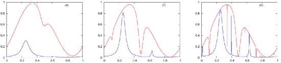
Figure 8.1: Invariant graphs for the $1$-parameter family $f_{\beta}(x,y)=(x+\rho,\arctan(\alpha y)-2\beta-\gamma(\sin(2\pi x)+1))$ where $\rho$ is the golden mean, $\alpha=100$, $\gamma=1/2$, and (a) $\beta=0.265$, (b) $\beta=0.275$, (c) $\beta=0.2753743$.

For all $\beta\geq 0$, the curves $\gamma^{-}\equiv 0$ and $\gamma^{+}\equiv 2$ satisfy $f^{\pm 1}_{\beta*}\gamma^{\pm}\leq\gamma^{\pm}$. Conditions $(r3)$–$(r7)$ and $(d3)$–$(d6)$ are obviously verified. In order to check $(r1)$, respectively $(d1)$, note that for all sufficiently large $\alpha$ (say, $\alpha\geq 20$), the curve $\psi$ given by $\psi(\theta)=\frac{3}{4}-\frac{1}{2}\sin(2\pi(\theta-\rho))$ satisfies $f_{0*}\psi\geq\psi$. As argued in the proof of Theorem 4.1, this implies the existence of two $f_{0}$-invariant graphs (compare (4.4)), whereas the non-existence of $f_{\beta_{1}}$-invariant graphs in $\Gamma$ can be seen from the fact that $f_{1,0}(2)<0$. Consequently (8.1) satisfies all assumptions of (the analogue version of) Theorems 4.1 and 6.1, and we obtain the existence of a saddle-node bifurcation in $\Gamma$. Figure 8.1 shows the approach of the upper and lower invariant graph in $\Gamma$. In (c), $\beta=0.2753743$ is a good approximation of the bifurcation point and the picture gives an idea of the strange non-chaotic attractor-repeller pair that emerges.

For slightly larger parameters $\beta$, the invariant graphs in $\Gamma$ disappear. In this case, all trajectories converge to an attracting continuous invariant graph, in the region below $\mathbb{T}^{1}\times\{0\}$, which exists throughout the whole parameter range.

In order to construct an example with a more complex bifurcation pattern, in the sense discussed at the end of Sections 4 and 6, we need a base transformation that exhibits more complicated dynamics and, in particular, a multitude of invariant measures and minimal sets. Evidently, the canonical choice is to use a two-dimensional transformation, since this allows at the same time for the required complex behaviour and a graphical representation of the invariant graphs of the resulting three-dimensional system. Our choice is the map

(8.2) $$\textstyle\omega(\theta_{1},\theta_{2})\ =\ \left(\theta_{1}+\frac{1}{2}\sin\left(2\pi\left(\theta_{2}+\frac{1}{2}\sin(2\pi\theta_{1})\right)\right),\theta_{2}+\frac{1}{2}\sin(2\pi\theta_{1})\right)\ ,$$

which has been studied in its own right in the context of quantum dynamics [21, 22].

It is known that $\omega$ has both an uncountable number of invariant ergodic measures and of minimal sets (this is due to the fact that its rotation set has non-empty interior, see [23] for a discussion). For the illustration, it is particularly convenient that $\omega$ exhibits four (star-shaped) elliptic islands, centred around the points of two period-2 orbits $M_{1}=\left\{\left(\frac{1}{4},\frac{1}{4}\right),\left(\frac{3}{4},\frac{3}{4}\right)\right\}$ and $M_{2}=\left\{\left(\frac{1}{4},\frac{3}{4}\right),\left(\frac{3}{4},\frac{1}{4}\right)\right\}$ (see Figure 8.2(a)).

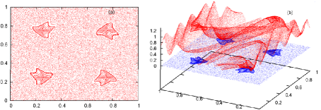
Figure 8.2: (a) Phase portrait of the map $\omega$ from (8.2). (b) The two invariant graphs at the bifurcation point $\beta_{c}\simeq 0.1855650809$ for the parametrised family $f_{\beta}(\theta,x)=(\omega(\theta),f_{\beta,\theta}(x))$ with $\omega$ from (8.2) and $f_{\beta,\theta}$ defined by (8.3).

As fibre maps, we choose

(8.3) $$\textstyle f_{\beta,\theta}(x)\ =\ \arctan(\alpha x)-2\beta-\gamma(\sin(2\pi\theta_{1})\sin(2\pi\theta_{2})+1)\ .$$

Note that for $\gamma>0$ the $\theta$-dependent term $-\gamma\sin(2\pi\theta_{1})\sin(2\pi\theta_{2})$ takes its global minimum exactly at the two points of the two-periodic orbit $M_{1}$. This implies that $M_{1}$ is the minimal set on which the first bifurcation occurs, that is, $\beta_{c}^{M_{1}}=\beta_{c}<\beta_{c}^{M}\ \forall\textrm{minimal sets }M\neq M_{1}$. Equivalently, $M_{1}$ is exactly the set of points on which the two invariant graphs touch at the bifurcation point. Furthermore, since $f_{\beta,\left(\frac{1}{4},\frac{1}{4}\right)}=f_{\beta,\left(\frac{3}{4},\frac{3}{4}\right)}$, the bifurcation pattern of $f_{\beta|M_{1}}$ is the same as the one of the one-dimensional family

$$g_{\beta}(x)\ =\ f_{\beta,\left(\frac{1}{4},\frac{1}{4}\right)}(x)\ =\ \arctan(\alpha x)-2\beta-2\gamma\ .$$

This allows to determine the precise bifurcation point, namely

(8.4) $$\beta_{c}\ =\ \frac{1}{2}\arctan(\sqrt{\alpha-1})-\frac{\sqrt{\alpha-1}}{2\alpha}-\gamma\ .$$

For $a=100$ and $\gamma=1/2$ we obtain $\beta_{c}\simeq 0.1855650809$.

Figure 8.2(b) shows the two invariant graphs in $\Gamma=\mathbb{T}^{2}\times[0,2]$ at this bifurcation point. The validity of the assumptions of Theorems 4.1 and 6.1 is checked in a similar way as in the previous example. The picture becomes clearer in Figure 8.3  where the restriction of the two invariant graphs over a neighbourhood of $\left(\frac{1}{4},\frac{1}{4}\right)$ is plotted, slightly before the bifurcation point in (a) and at the bifurcation point in (b).

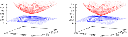
Figure 8.3: Closer view of the two invariant graphs over the islands ‘centred’ at the period $2$ point $(1/4,1/4)$. (a) $\beta=\beta_{c}-0.005$, (b) $\beta=\beta_{c}$.

Similarly to the previous example, there exists a third invariant graph below $\mathbb{T}^{2}\times\{0\}$, which is continuous and attracting and persists throughout the whole parameter range. Once the bifurcation has taken place over a minimal set $M$, this graph attracts all trajectories in $M\times[-5,2]$. Consequently, the upper bounding graph $\varphi^{+}_{M}$ ‘drops down’ from above 0 to below at the bifurcation point $\beta_{c}^{M}$. This happens first for $M_{1}$, and subsequently for all the invariant circles in the elliptic island, starting in the middle and moving outwards (see Figure 8.4(a)–(c)). Note that in all pictures in Figure 8.4 only the upper bounding graph is plotted, for the sake of better visibility.

When the outer boundary of the two elliptic islands containing $M_{1}$ is reached, the complement of the elliptic islands (the chaotic region in the sense of [23]) drops in one go. Finally, the invariant circles over the remaining two elliptic islands drop down one by one, in reversed order, moving inwards from the outside (note that on $M_{2}$ the $\theta$-dependent term takes its global maximum).

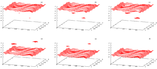
Figure 8.4: Invariant graphs for $f_{\beta}$ where $\alpha=100$, $\gamma=1/2$, and (a) $\beta=\beta_{c}+0.0005$, (b) $\beta=\beta_{c}+0.01$, (c) $\beta=\beta_{c}+0.0269$, (d) $\beta=\beta_{c}+0.02725$, (e) $\beta=\beta_{c}+0.485$, (f) $\beta=\beta_{c}+0.5$.

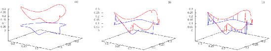
Figure 8.5: Closer view of two invariant circles above the island centred at the point $(1/4,1/4)$. Here, $\alpha=200$, $\gamma=1$, and (a) $\beta=\beta_{c}+0.0035$, (b) $\beta=\beta_{c}+0.03516$, (c) $\beta=\beta_{c}+0.035164103$. $\beta_{c}$ is again determined by (8.4). Note that $\beta_{c}$ is negative in this case. Hence, strictly speaking a reparametrisation would be necessary to meet the formal requirements of Theorem 6.1, but we omit the details.

Finally, in Figure 8.5, the bifurcation over one of the invariant circles of the elliptic island is shown. Although embedded in dimension two, the underlying dynamics are just those of an irrational rotation. Consequently, from a qualitative point of view, the situation is exactly the same as in the first example. Again, the non-uniform approach of the invariant circles can be observed, which is typical for the creation of strange non-chaotic attractors and repellers at the bifurcation point.

References

• [1] L. Arnold. Random Dynamical Systems. Springer, 1998.
• [2] R. Johnson, P. Kloeden, and R. Pavani. Two-step transition in non-autonomous bifurcations: an explanation. Stoch. Dyn., 2(1):67–92, 2002.
• [3] S. Novo, R. Obaya, and A.M. Sanz. Almost periodic and almost automorphic dynamics for scalar convex differential equations. Isr. J. Math., 144:157–189, 2004.
• [4] C. Núñez and R. Obaya. A non-autonomous bifurcation theory for deterministic scalar differential equations. Discrete Contin. Dyn. Syst., Ser. B, 9(3–4):701–730, 2007.
• [5] A.J. Homburg and T. Young. Hard bifurcations in dynamical systems with bounded random perturbations. Regul. Chaotic Dyn., 11(2):247–258, 2006.
• [6] H. Zmarrou and A.J. Homburg. Bifurcations of stationary measures of random diffeomorphisms. Ergodic Theory Dyn. Syst., 27(5):1651–1692, 2007.
• [7] H. Zmarrou and A.J. Homburg. Dynamics and bifurcations of random circle diffeomorphisms. Discrete Contin. Dyn. Syst., Ser. B, 10(2–3):719–731, 2008.
• [8] T. Jäger. The creation of strange non-chaotic attractors in non-smooth saddle-node bifurcations. Mem. Am. Math. Soc., 945:1–106, 2009.
• [9] T.Y. Nguyen, T.S. Doan, T. Jäger, and S. Siegmund. Saddle-node bifurcations in the quasiperiodically forced logistic map. Preprint, 2010.
• [10] G. Keller. A note on strange nonchaotic attractors. Fundam. Math., 151(2):139–148, 1996.
• [11] A.I. Alonso and R. Obaya. The structure ob the bounded trajectories set of a scalar convex differential equation. Proc. Roy. Soc. Edinburgh, 133(2):237–263, 2003.
• [12] J. Stark and R. Sturman. Semi-uniform ergodic theorems and applications to forced systems. Nonlinearity, 13(1):113–143, 2000.
• [13] P. Glendinning. Global attractors of pinched skew products. Dyn. Syst., 17:287–294, 2002.
• [14] J. Stark. Transitive sets for quasi-periodically forced monotone maps. Dyn. Syst., 18(4):351–364, 2003.
• [15] T. Jäger and J. Stark. Towards a classification for quasiperiodically forced circle homeomorphisms. J. Lond. Math. Soc., 73(3):727–744, 2006.
• [16] R. Fabbri, T. Jäger, R. Johnson, and G. Keller. A Sharkovskii-type theorem for minimally forced interval maps. Topol. Methods Nonlinear Anal., 26:163–188, 2005.
• [17] T. Jäger. Quasiperiodically forced interval maps with negative Schwarzian derivative. Nonlinearity 16(4):1239–1255, 2003.
• [18] A. Katok and B. Hasselblatt. Introduction to the Modern Theory of Dynamical Systems. Cambridge University Press, 1997.
• [19] J. Stark. Regularity of invariant graphs for forced systems. Ergodic Theory Dyn. Syst., 19(1):155–199, 1999.
• [20] C. Grebogi, E. Ott, S. Pelikan, and J.A. Yorke. Strange attractors that are not chaotic. Physica D, 13:261–268, 1984.
• [21] P. Leboeuf, J. Kurchan, M. Feingold and D.P. Arovas. Phase-space localization: topological aspects of quantum chaos. Phys. Rev. Lett., 65(25):3076–3079, 1990.
• [22] T. Geisel, R. Ketzmerick and G. Peschel. Metamorphosis of a Cantor spectrum due to classical chaos. Phys. Rev. Lett., 67(26):3635–3638, 1991.
• [23] T. Jäger. Elliptic stars in a chaotic night. Preprint 2010.