Incremental Refinement using a Gaussian
Test Channel

Abstract

The additive rate-distortion function (ARDF) was developed in order to universally bound the rate loss in the Wyner-Ziv problem, and has since then been instrumental in e.g., bounding the rate loss in successive refinements, universal quantization, and other multi-terminal source coding settings. The ARDF is defined as the minimum mutual information over an additive test channel followed by estimation. In the limit of high resolution, the ADRF coincides with the true RDF for many sources and fidelity criterions. In the other extreme, i.e., the limit of low resolutions, the behavior of the ARDF has not previously been rigorously addressed.

In this work, we consider the special case of quadratic distortion and where the noise in the test channel is Gaussian distributed. We first establish a link to the I-MMSE relation of Guo et al. and use this to show that for any source the slope of the ARDF near zero rate, converges to the slope of the Gaussian RDF near zero rate. We then consider the multiplicative rate loss of the ARDF, and show that for bursty sources it may be unbounded, contrary to the additive rate loss, which is upper bounded by 1/2 bit for all sources. We finally show that unconditional incremental refinement, i.e., where each refinement is encoded independently of the other refinements, is ARDF optimal in the limit of low resolution, independently of the source distribution. Our results also reveal under which conditions linear estimation is ARDF optimal in the low rate regime.

I Introduction

Shannon’s rate-distortion function (RDF) for a source $X$ and distortion measure $d(\cdot,\cdot)$ is given by

$$R(D)=\inf I(X;Y),$$ (1)

where the infimum is over all reconstructions $Y$ such that the expected distortion satisfies $\mathbb{E}[d(X,Y)]\leq D$. Even though (1) perhaps appears simple and innocent, it is well-known that it is generally very hard to explicitly compute. In fact, there exists only very few cases where (1) is known in closed-form, e.g., Gaussian sources and MSE, binary sources and Hamming distances etc. In the information theoretic literature, several methods have been proposed to approximate the RDF’s e.g., iterative numeric solutions, high-resolution source coding, and (universal) bounds. In the first case, the Arimoto-Blahut algorithm is able to numerically obtain the rate-distortion function for arbitrary finite input/output alphabet sources and single-letter distortion measures [1]. In the second case, for continuous alphabet sources, it was shown by Linder and Zamir that the Shannon lower bound (SLB) is asymptotically tight for norm-based distortion metrics [2]. Thus, at asymptotically high coding rates, the RDFs can be approximated by simple formulaes. In the third case, alternative RDFs, which are easier to compute and analyze, are used to bound the true RDFs. For example, at general resolution and for difference distortion measures, the SLB provides a lower bound to the true RDF for many sources. On the other hand, Zamir presented in [3] an additive RDF (ARDF), which consists of an additive test channel followed by estimation. The ARDF has been shown to be a convenient tool for upper bounding the rate loss in many source coding problems. In particular, it was shown in [3] that the additive rate loss in the Wyner-Ziv problem is at most 1/2 bit for all sources. Similarly, it was shown by Lastras and Berger in [4], that the additive rate loss in the successive refinement problem is at most 1/2 bit per stage. The ARDF has also been successfully applied to upper bound the rate loss in other multi-terminal problems, cf. [3, 5]. In the limit of high resolution, the ARDF coincides with the true RDF for many sources and fidelity criterions [2]. In the other extreme, i.e., in the limit of low resolutions, the behavior of the ARDF has not been rigorously addressed. There has, however, been a great interest in the counter part to low resolution source coding, i.e., communication at low SNR, e.g., ultra-wideband communication [6]. A motivating factor for considering the low SNR regime in communications, is that the absolute value of the slope of the capacity-cost function is large (and therefore small for the cost-capacity function), which indicates that one gets the most channel capacity per unit cost at low SNR, as was shown by Verdú [7]. Interestingly, Verdú also showed that for rate-distortion at low rates, the most cost effective operating point in terms of bits per unit distortion, is near zero rate [7]. This follows since the absolute value of the slope of the RDF is minimized when the distortion approaches its maximum.

In this paper, we are interested in analyzing the ARDF at low resolutions. We consider the special case of the ARDF where the test channel’s noise is Gaussian and the distortion measure is the MSE. We establish a link to the mutual information – minimum mean squared estimation (I-MMSE) relation of Guo et al. [8] and use this to show that for any source the slope of the ARDF near zero rate, converges to the slope of the Gaussian RDF near zero rate. We then consider the multiplicative rate loss of this ARDF and show that for bursty sources it may be unbounded. We also show that unconditional incremental refinement, i.e., where each refinement is encoded independently of the other refinements, is ARDF optimal in the limit of low resolution, independently of the source distribution. In particular, let an arbitrarily distributed source $X$ be encoded into $k$ representations $Y_{i}=\sqrt{\gamma}X+N_{i}$ where $\{N_{i}\},i=1,\dotsc,k,$ are mutually independent, Gaussian distributed, and independent of $X$. Then we show that $I(X;Y_{1},\dotsc,Y_{k})\approx\sum_{i}I(X;Y_{i})$ at low rates. Moreover, the joint reconstruction follows by simple linear estimation of $X$ from $\{Y_{1},\dotsc,Y_{k}\}$. If side information $Z$, where $Z$ is independent of $N_{i},i=1,\dotsc,k$, but arbitrarily jointly distributed with $X$, is available both at the encoder and decoder, we show that $I(X;Y_{1},\dotsc,Y_{k}|Z)\approx\sum_{i}I(X;Y_{i}|Z)$. In this case, however, the best conditional estimator $\mathbb{E}[X|Y_{1},\dotsc,Y_{k},Z]$ is generally not linear. We provide the exact conditions for ARDF optimality of linear estimation in the low rate regime.

II Background

In this section, we present two existing important concepts that we will be needing in the sequel, i.e., the additive RDF and the I-MMSE relation.

II-A The Additive Rate-Distortion Function

The additive (noise) RDF, as defined by Zamir in [3], describes the best rate-distortion performance achievable for any additive noise followed by optimum estimation, including the possibility of time sharing (convexification). In the current paper, we restrict attention to Gaussian noise, MMSE estimation (MSE distortion), and no time-sharing, so we take the “freedom” to use the notation additive RDF, $R_{X}^{\text{add}}(D)$, for this special case (i.e. no minimization over free parameters). Specifically, let $\mathrm{var}(X|Y)$ denote the minimum possible MSE in estimating $X$ from $Y$, i.e.,

$$\mathrm{var}(X|Y)\triangleq\mathbb{E}[(\mathbb{E}[X|Y]-X)^{2}].$$ (2)

Moreover, let the additive noise $N$ be zero-mean Gaussian distributed with variance $0<\theta<\infty$. Then,

$$R_{X}^{\text{add}}(D)=I(X;X+N),$$ (3)

where the noise variance $\theta$ is chosen such that $D=\mathrm{var}(X|X+N)$.

II-B The I-MMSE Relation

Using an incremental Gaussian channel, Guo et al. [8] was able to establish an explicit connection between information theory and estimation theory. For future reference, we include this result below:

Theorem 1 ([8]).

Let $N$ be zero-mean Gaussian of unit variance, independent of $X$, and let $X$ have an arbitrary distribution $P_{X}$ that satisfies $\mathbb{E}X^{2}<\infty$. Then

$$\frac{\mathrm{d}}{\mathrm{d}\gamma}I(X;\sqrt{\gamma}X+N)=\frac{\log_{2}(e)}{2}\mathrm{mmse}(\gamma),$$ (4)

where

$$\mathrm{mmse}(\gamma)=\mathbb{E}[(X-\mathbb{E}[X|\sqrt{\gamma}X+N])^{2}]=\mathrm{var}(X|\sqrt{\gamma}X+N).$$ (5)

III Incremental Refinements

III-A The Slope of the ARDF

We will show that the slope of $R_{X}^{\text{add}}(D)$ at $D=D_{\text{max}}$ for a source $X$ with variance $\sigma_{X}^{2}$ is independent of the distribution of $X$. In fact, the slope is identical to the slope of the RDF of a Gaussian source $X^{\prime}$ with variance $\sigma_{X^{\prime}}^{2}=\sigma_{X}^{2}$. This is interesting since the RDF of any zero-mean source $X$ with a variance $\mathrm{var}(X)=\sigma_{X}^{2}$ meets the Gaussian RDF at $D=D_{\text{max}}=\sigma_{X}^{2}$. Thus, since the Gaussian RDF can be obtained by linear estimation, it follows that $R_{X}^{\text{add}}(D)$ can also be obtained by linear estimation near $D_{\text{max}}$.

Lemma 1.

Let $Y=\sqrt{\gamma}X+N,$ where $N\small\raisebox{-1.13809pt}{\rotatebox{90.0}{$\models$}\,}X$, $X$ is arbitrarily distributed with variance $\sigma_{X}^{2}$ and $N$ is Gaussian distributed according to $\mathcal{N}(0,1)$. Moreover, let $R_{X}^{\text{add}}(D)$ be the additive RDF. Then

$$\lim_{D\to D_{\mathrm{max}}}\frac{\mathrm{d}}{\mathrm{d}D}R_{X}^{\text{add}}(D)=-\frac{\log_{2}(e)}{2\sigma_{X}^{2}},$$ (6)

irrespective of the distribution on $X$.

Remark 1.

Interestingly, it was shown by Marco and Neuhoff [9] that in the quadratic memoryless Gaussian case, the operational rate-distortion function of the scalar uniform quantizer (followed by entropy coding) has the same slope as (6). Thus, in this particular case, the optimal scalar quantizer is as good as any vector quantizer.

III-B Multiplicative Rate Loss in the Low Rate Regime

Recall that in e.g., the successive refinement problem, the additive rate loss is no more than 0.5 bits per stage. We will now show that the multiplicative rate loss may be unbounded.

Let $X$ be a Gaussian mixture source with a density $P_{X}(x)$ given by $P_{X}(x)=P_{0}\mathcal{N}(0,\sigma_{0}^{2})+P_{1}\mathcal{N}(0,\sigma_{1}^{2})$, where $P_{0}+P_{1}=1$. The variance $\sigma_{X}^{2}$ of $X$ is $\sigma_{X}^{2}=P_{0}\sigma_{0}^{2}+P_{1}\sigma_{1}^{2}$. The components contribution can be parametrized by $\lambda\in[0;1]$ as follows: $P_{0}\sigma_{0}^{2}=\lambda\sigma_{X}^{2},P_{1}\sigma_{1}^{2}=(1-\lambda)\sigma_{X}^{2}$. It will be convenient to let $\sigma_{X}^{2}=1$ and $\lambda=\frac{1}{2}$. Moreover, we shall assume that $\sigma_{1}^{2}>1>\sigma_{0}^{2}\geq\frac{1}{2}$. Notice that as $\sigma_{1}^{2}\to\infty$ we have that $P_{1}\to 0,P_{0}\to 1$, and $\sigma_{0}^{2}\to\frac{1}{2}$.

At this point, let $S=0$ with probability $P_{0}$ and $S=1$ with probability $P_{1}$, and let $S$ be an indicator of the two components, i.e., $X\sim\mathcal{N}(0,\sigma_{0}^{2})$, if $S=0$, and $X\sim\mathcal{N}(0,\sigma_{1}^{2})$, if $S=1$. The RDF, conditional on the indicator $S$, is given by

$$R_{X|S}(D)=\begin{cases}\frac{1}{2}\sum_{i\in\{0,1\}}P_{i}\log_{2}(\sigma_{i}^{2}/D),&\text{if $0<D\leq\sigma_{0}^{2}$},\\[14.22636pt] \displaystyle\frac{P_{1}}{2}\log_{2}\bigg{(}\frac{P_{1}\sigma_{1}^{2}}{D-P_{0}\sigma_{0}^{2}}\bigg{)},&\text{if $\sigma_{0}^{2}<D<1$}.\end{cases}$$

Thus, the slope of $R_{X|S}(D)$ w.r.t. $D$ is given by

$$\lim_{D\to\sigma_{X}^{2}}\frac{\mathrm{d}}{\mathrm{d}D}R_{X|S}(D) =-\frac{P_{1}}{4\ln(2)\sigma_{X}^{2}},$$ (7)

which tends to zero as $\sigma_{1}^{2}\to\infty$ and $P_{1}\to 0$. It follows from this fact and from Lemma 1 that the ratio of the slope of the conditional RDF and the slope of the ARDF grows unboundedly as $\sigma_{1}^{2}\to\infty$. Moreover, as $\sigma_{1}^{2}\to\infty$, $\sigma_{0}^{2}\to\frac{1}{2}$, which implies that it becomes increasingly easier for the uninformed encoder/decoder to guess the correct component of the source. Thus, the conditional RDF converges towards the true RDF $R_{X}(D)$, from which it follows that the ratio $\lim_{\sigma_{1}^{2}/\sigma_{0}^{2}\to\infty}\lim_{D\to\sigma_{X}^{2}}R_{X}^{\text{add}}(D)/R_{X}(D)\to\infty$.

III-C Unconditional Incremental Refinements

We will now show that unconditional incremental refinement, i.e., where each refinement is encoded independently of the other refinements, is ARDF optimal in the limit of low resolution, independently of the source distribution. This result is not only of theoretical value but is also useful in practice, since conditional source coding is generally more complicated than unconditional source coding, i.e., creating descriptions that are individually optimal and at the same time jointly optimal is a long standing problem in information theory, where it is known as the multiple descriptions problem [10].

Lemma 2.

Let $X$ be arbitrarily distributed with variance $\sigma_{X}^{2}$, and let $N_{i}\small\raisebox{-1.13809pt}{\rotatebox{90.0}{$\models$}\,}X,i=0,\dotsc,k-1,$ be a sequence of zero-mean mutually independent Gaussian sources each with variance $\sigma_{N}^{2}$. Then

$$I(X;X+N_{0},\dotsc,X+N_{k-1})=I(X;X+\frac{1}{\sqrt{k}}N_{0}).$$

Lemma 3.

Let $Y_{i}=\sqrt{\gamma}X+N_{i},i=0,\dotsc,k-1$, where $N_{i}\small\raisebox{-1.13809pt}{\rotatebox{90.0}{$\models$}\,}X,\forall i$. Moreover, let $X$ be arbitrarily distributed with variance $\sigma_{X}^{2}$ and let $N_{0},\dotsc,N_{k-1},$ be zero-mean unit-variance i.i.d. Gaussian distributed. Then

$$\lim_{\gamma\to 0}\frac{1}{\gamma}I(X;Y_{0},\dotsc,Y_{k-1}) =k\lim_{\gamma\to 0}\frac{1}{\gamma}I(X;\sqrt{\gamma}X+N_{0})$$

$$=\frac{k\log_{2}(e)}{2}\sigma_{X}^{2}$$

and

$$\lim_{\gamma\to 0}\frac{1}{\gamma}\bigg{[}\frac{1}{\mathrm{var}(X|Y_{1},\dotsc,Y_{k-1})}-\frac{1}{\sigma_{X}^{2}}\bigg{]}=k.$$ (8)

To illustrate the importance of Lemma 3, let us consider the situation of a zero-mean unit-variance memoryless Gaussian source $X$, which is to be encoded successively in $M$ stages. In stage $i$, $L$ descriptions $Y_{i,j},j=1,\dotsc,L$, are constructed unconditionally of each other. Thus, for the same coding rate (at each stage), the joint distortion $\mathrm{var}(X|Y_{1,1},\dotsc,Y_{1,L},\dotsc,Y_{i,1},\dotsc,Y_{i,L})$ in the $i$th stage is worse than if only a single joint description within each stage had been created. In fact, in the symmetric case where all individual descriptions within stage $i$ has the same distortion $d_{i}$ and rate $r_{i}$, it can be shown that the joint distortion $D_{i}$ of the $i$th stage is given by

$$D_{i}=\frac{d_{i}}{L-(L-1)d_{i}/D_{i-1}}$$ (9)

and the sum-rate at stage $i$ is given by

$$R_{i}=L\sum_{j=1}^{i}r_{i}=L\sum_{j=1}^{i}\frac{1}{2}\log_{2}(D_{j-1}/d_{j}),$$ (10)

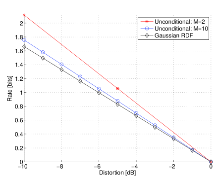
where $D_{0}=d_{0}=\sigma_{X}^{2}$. Since the Gaussian source is successively refinable, using conditional refinements will achieve the true RDF given by $R_{i}^{*}=\frac{1}{2}\log_{2}(1/D_{i})$, where $D_{i}$ is given by (9). On the other hand, the rate required when unconditional coding is used is given by (10). For comparison, we have illustrated the performance of unconditional and conditional coding when the source is encoded into $L=2$ descriptions per stage, for the case of of $M=2$ and $M=10$ increments (stages), respectively, see Fig. 1. In this example, $\sigma_{X}^{2}=1$ and $D_{M}=0.1$. Notice that when using smaller increments, i.e., when $M=10$ as compared to when $M=2$, the resulting rate loss due to using unconditional coding is significantly reduced.

Figure 1: Unconditional and conditional successive refinements in the quadratic Gaussian case.

III-D Unconditional Incremental Refinements (Side Information)

The case of additional side information available at the encoder and the decoder was not considered by Guo et al. in [8]. Below we generalize Theorem 1 to include side information:

Lemma 4.

Let $Y=\sqrt{\gamma}X+N$ where $N\sim\mathcal{N}(0,1)$ and $X$ is arbitrarily distributed, independent of $N$ and of variance $\sigma_{X}^{2}$. Let $Z$ be arbitrarily distributed and correlated with $X$ but independent of $N$. Then

$$\lim_{\gamma\to 0}\frac{1}{\gamma}I(X;Y|Z)=\frac{\log_{2}(e)}{2}\mathrm{var}(X|Z).$$ (11)

Corollary 1.

Let $Y_{i}=\sqrt{\gamma}X+N_{i},i=0,\dotsc,k-1$, where $N_{i}\small\raisebox{-1.13809pt}{\rotatebox{90.0}{$\models$}\,}X,\forall i,$ and $N_{0},\dotsc,N_{k-1}$. Let $X$ be arbitrarily distributed with variance $\sigma_{X}^{2}$ and let $N_{0},\dotsc,N_{k-1},$ be zero-mean unit-variance i.i.d. Gaussian distributed. Let $Z$ be arbitrarily distributed and correlated with $X$ but independent of $N_{i},\forall i$. Then

$$\lim_{\gamma\to 0}\frac{1}{\gamma}I(X;Y_{0},\dotsc,Y_{k-1}|Z) =\frac{k\log_{2}(e)}{2}\mathrm{var}(X|Z).$$

III-E Conditions for Optimality of Linear Estimation

It was recently shown by Akyol et al. [11], that for an arbitrarily distributed source $X$, contaminated by Gaussian noise $N$, the MMSE estimator of $X$ given $Y=\sqrt{\gamma}X+N$, converges in probability to a linear estimator, in the limit where $\gamma\to 0$. Contrary to this result, we show that the conditional MMSE estimator $\mathbb{E}[X|Y,Z]$ with side information $Z$, where $Z$ is independent of $N$ but is arbitrarily correlated with $X$ is generally not linear.

Lemma 5.

Let $Y=\sqrt{\gamma}X+N,$ where $N\small\raisebox{-1.13809pt}{\rotatebox{90.0}{$\models$}\,}X$, $X$ is arbitrarily distributed with variance $\sigma_{X}^{2}$ and $N$ is Gaussian distributed according to $\mathcal{N}(0,1)$. Moreover, let $Z$ be arbitrarily distributed, independent of $N$ but arbitrarily correlated with $X$. Then the conditional MMSE estimator $\mathbb{E}[X|Y,Z]$ is linear if and only if

$$\mathbb{E}[\mathrm{var}(X|Z=z)^{2}]=\mathrm{var}(X|Z)^{2},$$ (12)

where

$$\mathbb{E}[\mathrm{var}(X|Z=z)^{2}]\triangleq\mathbb{E}_{Z}[(\mathbb{E}_{X}[(\mathbb{E}_{X}[X|Z=z]-X)^{2}])^{2}]$$

and

$$\mathrm{var}(X|Z)^{2}\triangleq(\mathbb{E}_{X}[(\mathbb{E}_{X}[X|Z]-X)^{2}])^{2}.$$

In the case where $X,Z$ are jointly Gaussian, it is easy to show that (12) is satisfied and, thus, the MMSE estimator $\mathbb{E}[X|Y,Z]$ is trivially linear in both $Z$ and $N$.

References

- [1] R. E. Blahut, “Computation of channel capacity and rate-distortion function,” IEEE Trans. Inform. Theory, no. 4, pp. 460 – 473, July 1972.
- [2] T. Linder and R. Zamir, “On the asymptotic tightness of the Shannon lower bound,” IEEE Trans. Inform. Theory, vol. 40, no. 6, pp. 2026 – 2031, November 1994.
- [3] R. Zamir, “The rate loss in the Wyner-Ziv problem,” IEEE Trans. Inform. Theory, vol. 42, no. 6, pp. 2073 – 2084, November 1996.
- [4] L. Lastras and T. Berger, “All sources are nearly successively refinable,” IEEE Trans. Inform. Theory, vol. 47, no. 3, pp. 918 – 926, 2001.
- [5] R. Zamir and T. Berger, “Multiterminal source coding with high resolution,” IEEE Trans. Inform. Theory, vol. 45, no. 1, pp. 106 – 117, January 1999.
- [6] A. Lapidoth and I. E. Teletar, “On wide-band broadcast channels,” IEEE Trans. Inform. Theory, vol. 49, no. 12, pp. 3250 – 3258, December 2003.
- [7] S. Verdú, “On channel capacity per unit cost,” IEEE Trans. Inform. Theory, no. 5, pp. 1019 – 1030, September 1990.
- [8] D. Guo, S. Shamai, and S. Verdú, “Mutual information and minimum mean-square error in Gaussian channels,” IEEE Trans. Inform. Theory, vol. 51, pp. 1261 – 1282, April 2005.
- [9] D. Marco and D. L. Neuhoff, “Low-resolution scalar quantization for Gaussian sources and squared error,” IEEE Trans. Inform. Theory, vol. 52, no. 4, pp. 1689 – 1697, April 2006.
- [10] A. A. E. Gamal and T. M. Cover, “Achievable rates for multiple descriptions,” IEEE Trans. Inform. Theory, vol. IT-28, no. 6, pp. 851 – 857, Nov. 1982.
- [11] E. Akyol, K. Viswanatha, and K. Rose, “On conditions for linearity of optimal estimation,” in IEEE Information Theory Workshop, Dublin, 2010.