Abstract

A waveguide coincides with a strip having two narrows of diameter $\varepsilon$. Electron motion is described by the Helmholtz equation with Dirichlet boundary condition. The part of waveguide between the narrows plays the role of resonator and there can occur electron resonant tunneling. This phenomenon consists in the fact that, for an electron with energy $E$, the probability $T(E)$ to pass from one part of the waveguide to the other part through the resonator has a sharp peak at $E=E_{res}$, where $E_{res}$ denotes a ”resonant” energy. In the present paper, we compare the asymptotics of $E_{res}=E_{res}(\varepsilon)$ and $T(E)=T(E,\varepsilon)$ as $\varepsilon\to 0$ with the corresponding numerical results obtained by approximate computing the waveguide scattering matrix. We show that there exists a band of $\varepsilon$ where the asymptotics and numerical results are in close agreement. The numerical calculations become inefficient as $\varepsilon$ decreases; however, at such a condition the asymptotics remains reliable. On the other hand, the asymptotics gives way to the numerical method as $\varepsilon$ increases; in fact, for wide narrows the resonant tunneling vanishes by itself.

Though, in the present paper, we consider only a 2D waveguide, the applicability of the methods goes far beyond the above simplest model. In particular, the same approach will work for asymptotic and numerical analysis of resonant tunneling in 3D quantum waveguides.

1 Introduction

As an electron propagates in a quantum waveguide of variable cross-section, the waveguide narrows play the role of effective potential barriers for the longitudinal motion. The part of the waveguide between two narrows becomes a ”resonator” , and there can arise resonant tunneling. It consists of the fact that, for an electron with energy $E$, the probability $T(E)$ to pass from one part of the waveguide to the other through the resonator has a sharp peak at $E=E_{res}$, where $E_{res}$ denotes a resonant energy. There are prospects for building a new class of nanosize electronics elements (transistors, electron energy monochromators, key devices) based on the phenomenon of resonant tunneling. To analyze their operation, it is important to know $E_{res}$, the height of the resonant peak, the behavior of $T(E)$ for $E$ close to $E_{res}$, etc.

In [1], electron propagation was considered in a 3D waveguide with two cylindrical outlets to infinity and two narrows of small diameter $\varepsilon_{1}$ and $\varepsilon_{2}$. The electron motion was described by the Helmholtz equation with Dirichlet boundary condition, radiation condition, and a wave number $k$ between the first and the second thresholds. For the aforementioned characteristics of resonant tunneling, there were obtained asymptotics as $\varepsilon_{1},\varepsilon_{2}\to 0$. The asymptotic formulas provide mainly a qualitative picture. In the present paper, we show that, being supplemented by some computations, the asymptotics can tell a useful quantitative information as well. Though the paper continues the studies in [1], nevertheless it is practically self-contained; let us explain its goal in detail.

The asymptotic formulas in [1] include several unknown constant coefficients, which can be found by solving some boundary value problems independent of $\varepsilon_{1}$ and $\varepsilon_{2}$. Here, in a model situation, we calculate approximately such coefficients, which enables us to take the asymptotics as numerical values of resonant tunneling characteristics for sufficiently small $\varepsilon_{1}$ and $\varepsilon_{2}$. This leads to the question which $\varepsilon_{1}$, $\varepsilon_{2}$ could be considered as ”sufficiently small” ; in other words, where does the asymptotics work in a proper way? Though there is no universal answer for such a question, some examples give a grasp of what should be expected in analogous cases. To this end we calculate (also approximately) the scattering matrix and then compare the results obtained by the asymptotic and computational methods independently of one another. Generally, it can be predicted that numerical calculations will become inefficient as the narrow diameters decrease and the resonant peak turns out to be ”too sharp” ; however, at such a condition the asymptotics should become more reliable. On the other hand, the asymptotics will give way to the numerical method as the narrow diameters increase; in fact, for wide narrows the resonant tunneling would vanish by itself. We observe these phenomena and show that there exists a band of the diameters, where the asymptotic and numerical approaches give compatible results.

In the present paper, we consider a 2D waveguide that is a strip with two narrows of the same diameter $\varepsilon$ (see Fig. 2). For 2D waveguides, the asymptotics of resonant tunneling characteristics (as $\varepsilon\to 0$) are published here for the first time; however, we do not prove the formulas in the paper. The reader could obtain the needed proofs by modifying arguments in [1] related to a 3D situation. Nonetheless, we analyze the structure of asymptotics in order to explain what constants in the asymptotic formulas have to be calculated numerically and how to do that by solving some boundary value problems independent of $\varepsilon$.

The paper consists of five sections. The mathematical model of the waveguide and statement of the problem are given in section 2. The asymptotic formulas are presented in section 3. Then, in section 4, we list the constants to be calculated in the asymptotics, describe the boundary value problems needed for the purpose, and present the methods for solving the problems numerically. In the same section we also describe a method we have used for approximate computation of the waveguide scattering matrix. Finally, section 5 is devoted to comparing basic resonant tunneling characteristics obtained in two different ways, asymptotic and numerical, independent of one another.

Though in the present paper we considered only a 2D waveguide, the applicability of the methods goes far beyond the above simplest model. In particular, the same approach will work for comparison asymptotic and numerical analysis of resonant tunneling in 3D quantum waveguides.

2 Statement of the problem

To describe the domain $G(\varepsilon)$ in $\mathbb{R}^{2}$ occupied by the waveguide, we first introduce two auxiliary domains $G$ and $\Omega$ in $\mathbb{R}^{2}$. The domain $G$ is the strip

$$G=\mathbb{R}\times D=\{(x,y)\in\mathbb{R}^{2}:x\in\mathbb{R}=(-\infty,+\infty);y\in D=(-l/2,l/2)\}.$$

Let us define $\Omega$. Denote by $K$ a double cone with vertex at the origin $O$ that contains the $x$-axis and is symmetric about the coordinate axes. The set $K\cap S^{1}$, where $S^{1}$ is a unit circle, consists of two simple arcs. Assume that $\Omega$ contains the cone $K$ and a neighborhood of its vertex; moreover, outside a large disk (centered at the origin) $\Omega$ coincides with $K$. The boundary $\partial\Omega$ of $\Omega$ is supposed to be smooth (see Fig. 1).

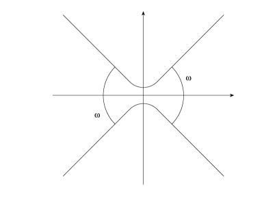
Figure 1: The set $\Omega$.

We now turn to the waveguide $G(\varepsilon)$. Denote by $\Omega(\varepsilon)$ the domain obtained from $\Omega$ by the contraction with center at $O$ and coefficient $\varepsilon$. In other words, $(x,y)\in\Omega(\varepsilon)$ if and only if $(x/\varepsilon,y/\varepsilon)\in\Omega$. Let $K_{j}$ and $\Omega_{j}(\varepsilon)$ stand for $K$ and $\Omega(\varepsilon)$ shifted by the vector $\mathbf{r}_{j}=(x_{j}^{0},0)$, $j=1,2$. We assume that $|x_{1}^{0}-x_{2}^{0}|$ is sufficiently large so the distance from $\partial K_{1}\cap\partial K_{2}$ to $G$ is positive. We put

$$G(\varepsilon)=G\cap\Omega_{1}(\varepsilon)\cap\Omega_{2}(\varepsilon)$$

(see Fig. 2).

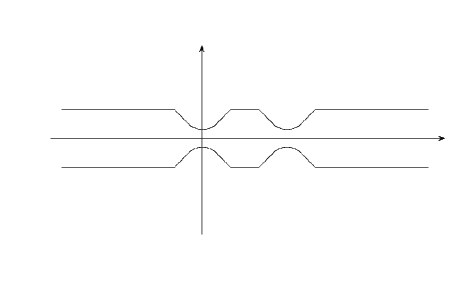
Figure 2: The waveguide $G(\varepsilon).$

The wave function of a free electron of energy $k^{2}$ satisfies the boundary value problem

$$\Delta u(x,y)+k^{2}u(x,y) = 0,\qquad(x,y)\in G(\varepsilon),$$ (2.1)

$$u(x,y) = 0,\qquad(x,y)\in\partial G(\varepsilon).$$

Moreover, $u$ is subject to radiation conditions at infinity. To formulate the conditions we need the problem

$$\Delta v(y)+\lambda^{2}v(y) = 0,\qquad y\in D,$$ (2.2)

$$v(-l/2)=v(l/2) = 0.$$

The eigenvalues $\lambda^{2}_{q}$ of this problem, where $q=1,2,\ldots$ are called the thresholds; they form the sequence $\lambda^{2}_{q}=(\pi q/l)^{2}$, $q=1,2,\ldots$. We suppose that $k^{2}$ in (2.1) is not a threshold. Given a real $k$, there exist finitely many linearly independent bounded wave functions. In the linear space spanned by such functions, a basis is formed by the wave functions subject to the radiation conditions

$$u_{m}(x,y) = \begin{cases}e^{i\nu_{m}x}\Psi_{m}(y)+\displaystyle\sum_{j=1}^{M}s_{mj}(k)\,e^{-i\nu_{j}x}\Psi_{j}(y)+O(e^{\delta x}),&x\rightarrow-\infty,\\ \displaystyle\sum_{j=1}^{M}s_{m,M+j}(k)\,e^{i\nu_{j}x}\Psi_{j}(y)+O(e^{-\delta x}),&x\rightarrow+\infty;\\ \end{cases}$$ (2.3)

$$u_{M+m}(x,y) = \begin{cases}\displaystyle\sum_{j=1}^{M}s_{M+m,j}(k)\,e^{-i\nu_{j}x}\Psi_{j}(y)+O(e^{\delta x}),&x\rightarrow-\infty,\\ e^{-i\nu_{m}x}\Psi_{m}(y)+\\ \hskip 34.14322pt+\displaystyle\sum_{j=1}^{M}s_{M+m,M+j}(k)\,e^{i\nu_{j}x}\Psi_{j}(y)+O(e^{-\delta x}),&x\rightarrow+\infty.\\ \end{cases}$$

Here $M$ is the number of the thresholds satisfying $\lambda^{2}<k^{2}$; $m=1,2,\ldots,M$; $\nu_{m}=\sqrt{k^{2}-\lambda^{2}_{m}}$; $\Psi_{m}$ is an eigenfunction of the problem (2.2) that corresponds to the eigenvalue $\lambda^{2}_{m}$ and is chosen so that

$$\Psi_{m}(y)=\left\{\begin{array}[]{ll}\sqrt{2/l\nu_{m}}\sin\lambda_{m}y,&\hbox{$m$ even,}\\ \sqrt{2/l\nu_{m}}\cos\lambda_{m}y,&\hbox{$m$ odd.}\\ \end{array}\right.$$ (2.4)

The function $U_{j}(x,y)=e^{i\nu_{j}x}\Psi_{j}(y),\qquad j=1,\ldots,M$, in the strip $G$ is a wave incoming from $-\infty$ and outgoing to $+\infty$, while $U_{M+j}(x,y)=e^{-i\nu_{j}x}\Psi_{j}(y),\qquad j=1,\ldots,M,$ is a wave going from $+\infty$ to $-\infty$. The scattering matrix

$$S=\|s_{mj}\|_{m,j=1,\ldots,2M}$$

is unitary. The values

$$R_{m}=\sum_{j=1}^{M}|s_{mj}|^{2},\qquad\,\,\,T_{m}=\sum_{j=1}^{M}|s_{m,\,M+j}|^{2}$$

are called the reflection and transition coefficients, relatively, for the wave $U_{m}$ incoming to $G(\varepsilon)$ from $-\infty$, $m=1,\dots,M$. (Similar definitions can be given for the wave $U_{M+m}$ coming from $+\infty$.)

In the present work we will discuss only the case $(\pi/l)^{2}<k^{2}<(2\pi/l)^{2}$, i.e., $k^{2}$ is between the first and the second thresholds. Then the scattering matrix is of size $2\times 2$. We consider only the scattering of the wave incoming from $-\infty$ and denote the reflection and transition coefficients as

$$R=R(k,\varepsilon)=|s_{11}(k,\varepsilon)|^{2},\qquad\,\,\,T=T(k,\varepsilon)=|s_{12}(k,\varepsilon)|^{2}.$$ (2.5)

The goal is to find a ”resonant” value $k_{r}=k_{r}(\varepsilon)$ of the parameter $k$ corresponding to the maximum of the transition coefficient, and to describe the behavior of $T(k,\varepsilon)$ for $k$ in a neighborhood of $k_{r}(\varepsilon)$ as $\varepsilon\to 0$.

3 Outline of the asymptotics

When deriving an asymptotics of a wave function (i.e. solution of problem (2.1)) as $\varepsilon\rightarrow 0$, we use the compound asymptotics method (the general theory of the method was exposed, e.g., in [2], [3]). To this end we introduce ”limit”  boundary value problems independent of the parameter $\varepsilon$. Put $G(0)=G\cap K_{1}\cap K_{2}$ (Fig. 3); thus, $G(0)$ consists of the three parts $G_{1}$, $G_{2}$, and $G_{3}$, where $G_{1}$ and $G_{3}$ are infinite domains while $G_{2}$ is a bounded resonator.

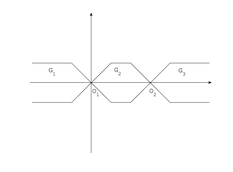
Figure 3: The set $G(0).$

The problems

$$\Delta v(x,y)+k^{2}v(x,y) = 0,\qquad(x,y)\in G_{j},$$ (3.1)

$$v(x,y) = 0,\qquad(x,y)\in\partial G_{j},$$

where $j=1,2,3$ and $\partial G_{j}$ is the boundary of $G_{j}$, are called the first kind limit problems. Solutions $v_{1}$ and $v_{3}$ are subject to some radiation conditions at infinity and all three functions $v_{1}$, $v_{2}$, $v_{3}$ satisfy some conditions at the corner points. All of the conditions will be formulated as required.

Let us turn to the domains $\Omega_{1}$ and $\Omega_{2}$ (see Fig. 1). Problems of the form

$$\Delta w(\xi_{j},\eta_{j}) = F(\xi_{j},\eta_{j})\qquad\hbox{in}\;\Omega_{j},$$ (3.2)

$$w(\xi_{j},\eta_{j}) = 0\qquad\qquad\quad\hbox{on}\;\partial\Omega_{j},$$

are called the second kind limit problems. We seek solutions of the problems satisfying

$$w(\xi_{j},\eta_{j})=O\left(\rho_{j}^{-3\pi/\omega_{j}}\right)\qquad\hbox{as}\;\rho_{j}\rightarrow\infty;$$

here $(\xi_{j},\eta_{j})$ are rectangular coordinates with origin at the vertex $O_{j}$ of $K_{j}$, $\rho_{j}$ being the distance from $(\xi_{j},\eta_{j})$ to $O_{j}$ and $\omega_{j}$ the opening of $K_{j}$, $j=1,2$.

In the waveguide $G(\varepsilon)$, we consider the scattering of the wave $U(x,y)=e^{i\nu_{1}x}\Psi_{1}(y)$ incoming from $-\infty$ (see (2.4)). The asymptotics of the wave function is the main technical result. Although rather cumbersome, it will lead to much more explicit characteristics of the process. The wave function admits the representation

$$u(x,y;\varepsilon)=\chi_{1,\,\varepsilon}(x,y)v_{1}(x,y;\varepsilon)+$$

$$+\Theta(r_{1})w_{1}(\varepsilon^{-1}x_{1},\varepsilon^{-1}y_{1};\varepsilon)+\chi_{2,\,\varepsilon}(x,y)v_{2}(x,y;\varepsilon)+$$ (3.3)

$$+\Theta(r_{2})w_{2}(\varepsilon^{-1}x_{2},\varepsilon^{-1}y_{2};\varepsilon)+\chi_{3,\,\varepsilon}(x,y)v_{3}(x,y;\varepsilon)+R(x,y;\varepsilon).$$

Let us explain the notation and the structure of this formula. When composing the formula, we first describe the behavior of the wave function to the right of the narrows, where the wave function can be approximated by a solution $v_{3}$ of the problem (3.1) in $G_{3}$. The solution is subject to the radiation condition

$$v_{3}(x,y;\varepsilon)\sim s_{12}(\varepsilon)e^{i\nu_{1}x}\Psi_{1}(y)\qquad\hbox{as}\;x\rightarrow+\infty,$$ (3.4)

the element $s_{12}(\varepsilon)$ of scattering matrix being yet unknown. Problem (3.1) does not contain $\varepsilon$, nevertheless $v_{3}$ depends on the parameter because of $s_{12}(\varepsilon)$. By $\chi_{3,\,\varepsilon}$ we denote a cut-off function defined by

$$\chi_{3,\,\varepsilon}(x,y)=\left(1-\Theta(r_{2}/\varepsilon)\right)\mathbf{1}_{G_{3}}(x,y),$$

where $r_{2}=\sqrt{x_{2}^{2}+y_{2}^{2}}$ and $(x_{2},y_{2})$ are the coordinates of a point $(x,y)$ in the system obtained by shifting the origin to the point $O_{2}$; $\mathbf{1}_{G_{3}}$ is the indicator of $G_{3}$ (equal to 1 in $G_{3}$ and to 0 outside $G_{3}$); $\Theta(\rho)$ is a smooth non-negative function on the half-axis $0\leqslant\rho<+\infty$ that equals 1 as $0\leqslant\rho\leqslant\delta$ and vanishes as $\rho\geqslant 2\delta$ ($\delta$ being a fixed small positive number). Thus $\chi_{3,\varepsilon}$ is defined on the whole waveguide $G(\varepsilon)$ as well as the function $\chi_{3,\,\varepsilon}v_{3}$ in (3).

Being substituted to (2.1), the function $\chi_{3,\,\varepsilon}v_{3}$ gives a discrepancy in the right-hand side of the Helmholtz equation; the discrepancy is supported near the second narrow (to the right of it). We compensate the principal part of the discrepancy by means of the second kind limit problem in the domain $\Omega_{2}$. Namely, the discrepancy is rewritten into coordinates $(\xi_{2},\eta_{2})$ in $\Omega_{2}$ and is taken as a right-hand side for the Laplace equation. The solution $w_{2}$ of the corresponding problem (3.2) has to be rewritten into coordinates $(x_{2},y_{2})$ and multiplied by a cut-off function. As a result, there arises the term $\Theta(r_{2})w_{2}(\varepsilon^{-1}x_{2},\varepsilon^{-1}y_{2};\varepsilon)$ in (3).

Now we substitute the sum of two obtained terms into (2.1). The principal part of the corresponding discrepancy is supported in $G_{2}$ near the second narrow. We compensate it by solving the problem (3.1) in $G_{2}$ and obtain the term $\chi_{2,\,\varepsilon}(x,y)v_{2}(x,y;\varepsilon)$ with

$$\chi_{2,\,\varepsilon}(x,y)=\left(1-\Theta(\varepsilon^{-1}r_{1})-\Theta(\varepsilon^{-1}r_{2})\right)\mathbf{1}_{G_{2}}(x,y).$$

Then in a similar way there arise

$$\Theta(r_{1})w_{1}(\varepsilon^{-1}x_{1},\varepsilon^{-1}y_{1};\varepsilon)\,\,{\rm and}\,\,\chi_{1,\,\varepsilon_{1}}(x,y)v_{1}(x,y;\varepsilon).$$

At the last step, we find the function $v_{1}$ that satisfies both the limit problem (3.1) in $G_{1}$ and the radiation condition

$$v_{1}(x,y;\varepsilon)\sim s_{12}(\varepsilon)\alpha(\varepsilon)e^{i\nu_{1}x}\Psi_{1}(y)+s_{12}(\varepsilon)\beta(\varepsilon)e^{-i\nu_{1}x}\Psi_{1}(y)$$

as $x\rightarrow-\infty$. The coefficients $\alpha$, $\beta$ and the entries $s_{11}$, $s_{12}$ of the scattering matrix turn out to be uniquely determined by a relation between $\alpha$ and $\beta$ that assures compensation of the principal part of the discrepancy arising in the problem in $G_{1}$, and by requirements

$$s_{12}(\varepsilon)\alpha(\varepsilon)=1,\quad s_{12}(\varepsilon)\beta(\varepsilon)=s_{11}(\varepsilon).$$

The remainder $R(x,y;\varepsilon)$ is small in comparison with the principal part of (3) as $\varepsilon\rightarrow 0$.

We specify (3) provided $k^{2}$ varies in an interval containing a unique simple eigenvalue $k^{2}_{0}$ of the problem (3.1) in $G_{2}$.

1. Introduce a special solution $\textbf{v}_{3}$ of the problem (3.1) in $G_{3}$ satisfying

   $$\textbf{v}_{3}(x,y)\sim(r_{2}^{-\pi/\omega}+ar_{2}^{\pi/\omega})\Phi(\varphi_{2})\qquad\hbox{as}\;r_{2}\rightarrow 0$$

   (here and below, $(r_{j},\varphi_{j})$ are polar coordinates with center at $O_{j}$, $j=1,2$; $\Phi(\varphi)=\cos(\pi\varphi/\omega)$), and

   $$\textbf{v}_{3}(x,y)\sim Ae^{i\nu_{1}x}\Psi_{1}(y)\qquad\hbox{as}\;x\rightarrow+\infty.$$

   These conditions define $\textbf{v}_{3}$ uniquely. The constants $a$, $A$ (depending on $k$ and on the geometry of $G_{3}$) have to be calculated. We have

   $$v_{3}(x,y;\varepsilon)=\frac{s_{12}(\varepsilon)}{A}\textbf{v}_{3}(x,y).$$

2. Consider a solution $w_{r}$ of the homogeneous problem (3.2) satisfying

   $$w_{r}(\xi,\eta)=\left\{\begin{array}[]{ll}(\rho^{\pi/\omega}+\alpha\rho^{-\pi/\omega})\Phi(\varphi)+O(\rho^{-3\pi/\omega}),&\hbox{as $\rho\rightarrow\infty$, $\xi>0$;}\\ \beta\rho^{-\pi/\omega}\Phi(\pi-\varphi)+O(\rho^{-3\pi/\omega}),&\hbox{as $\rho\rightarrow\infty$, $\xi<0$.}\\ \end{array}\right.$$ (3.5)

   The constants $\alpha$, $\beta$ (depending on $\Omega$) have to be calculated. One can prove that $\beta\neq 0$ (cf. [1], proof of Proposition 3.4). We put

   $$\textbf{w}^{-}(\xi,\eta) = \frac{1}{\beta}\left(w_{r}(\xi,\eta)-\zeta_{r}(\xi,\eta)(\rho^{\pi/\omega}+\alpha\rho^{-\pi/\omega})\Phi(\varphi)-\zeta_{l}(\xi,\eta)\beta\rho^{-\pi/\omega}\Phi(\pi-\varphi)\right),$$

   where $\zeta_{r}$ is a cut-off function equal to $1-\Theta$ as $\xi>0$ and 0 as $\xi<0$, $\zeta_{l}(\xi,\eta)=\zeta_{r}(-\xi,\eta)$. We also put

   $$\textbf{w}^{+}(\xi,\eta)=\beta\textbf{w}^{-}(-\xi,\eta)-\alpha\textbf{w}^{-}(\xi,\eta).$$

   Then

   $$w_{2}(\xi_{2},\eta_{2};\varepsilon)=\frac{s_{12}(\varepsilon)}{A}\left(\varepsilon^{-\pi/\omega}\textbf{w}^{-}(\xi_{2},\eta_{2})+a\varepsilon^{\pi/\omega}\textbf{w}^{+}(\xi_{2},\eta_{2})\right).$$

3. Remind that $k^{2}_{0}$ is a simple eigenvalue. Let $v_{0}$ be an eigenfunction corresponding to $k^{2}_{0}$ and normalized by $\int_{G_{2}}|v_{0}|^{2}dx\,dy=1$. We have

   $$v_{0}(x,y)\sim\left\{\begin{array}[]{ll}b_{1}r_{1}^{\pi/\omega}\Phi(\varphi_{1}),&\hbox{as $r_{1}\rightarrow 0$;}\\ b_{2}r_{2}^{\pi/\omega}\Phi(\pi-\varphi_{2}),&\hbox{as $r_{2}\rightarrow 0$.}\\ \end{array}\right.$$ (3.6)

   In what follows we assume that $b_{1}\neq 0$; such an assumption is fulfilled, for example, if $k^{2}_{0}$ is the first eigenvalue of problem (3.1). Since $G_{2}$ is invariant with respect to the transformation $(x,y)\mapsto(d-x,y)$, while $d=|x^{0}_{1}-x^{0}_{2}|$ is the distance between $O_{1}$ and $O_{2}$, one can prove that $q:=b_{2}/b_{1}=\pm 1$. Introduce special solutions $\textbf{v}_{21}$, $\textbf{v}_{22}$ of the problem (3.1) in $G_{2}$ satisfying

   $$\textbf{v}_{21}(x,y) \sim \left\{\begin{array}[]{ll}\left((k^{2}-k_{0}^{2})r_{1}^{-\pi/\omega}+c_{1}r_{1}^{\pi/\omega}\right)\Phi(\varphi_{1}),&\hbox{as $r_{1}\rightarrow 0$;}\\ c_{2}r_{2}^{\pi/\omega}\Phi(\pi-\varphi_{2}),&\hbox{as $r_{2}\rightarrow 0$,}\\ \end{array}\right.$$

   $$\textbf{v}_{22}(x,y) \sim \left\{\begin{array}[]{ll}\left(b_{2}r_{1}^{-\pi/\omega}+d_{1}r_{1}^{\pi/\omega}\right)\Phi(\varphi_{1}),&\hbox{as $r_{1}\rightarrow 0$;}\\ \left(-b_{1}r_{2}^{-\pi/\omega}+d_{2}r_{2}^{\pi/\omega}\right)\Phi(\pi-\varphi_{2}),&\hbox{as $r_{2}\rightarrow 0$.}\\ \end{array}\right.$$

   The coefficients $c_{1}$, $c_{2}$, $d_{1}$, $d_{2}$ depend on $k$ and on $G_{2}$. One can prove that $c_{j}(k_{0})=b_{1}b_{j}$. Then

   $$v_{2}(x,y;\varepsilon)=\frac{s_{12}(\varepsilon)}{b_{1}c_{2}}\bigl{(}(b_{1}\gamma(\varepsilon)-d_{2}\delta(\varepsilon))\textbf{v}_{21}(x,y)+c_{2}\delta(\varepsilon)\textbf{v}_{22}(x,y)\bigr{)},$$

   where

   $$\gamma(\varepsilon)=\frac{1}{A\beta}\left(\varepsilon^{-2\pi/\omega}-a\alpha\right),\qquad\delta(\varepsilon)=-\frac{1}{A\beta}\left(\alpha+a(\beta^{2}-\alpha^{2})\varepsilon^{2\pi/\omega}\right).$$ (3.9)

4. We have

   $$w_{1}(\xi_{1},\eta_{1};\varepsilon)=\dfrac{1}{|A|^{2}}\left((\overline{A}s_{11}(\varepsilon)+A)\varepsilon^{-\pi/\omega}\textbf{w}^{-}(\xi_{1},\eta_{1})+(a\overline{A}s_{11}(\varepsilon)+\overline{a}A)\varepsilon^{\pi/\omega}\textbf{w}^{+}(\xi_{1},\eta_{1})\right),$$

   where $s_{11}$ is defined by (3.10) below.

5. Introduce a special solution $\textbf{v}_{1}$ of the problem (3.1) in $G_{1}$ by $\textbf{v}_{1}(x_{1},y_{1})=\textbf{v}_{3}(d-x_{1},y_{1})$. Then

   $$v_{1}(x,y;\varepsilon)=\frac{s_{11}(\varepsilon)}{A}\textbf{v}_{1}(x,y)+\frac{1}{\overline{A}}\overline{\textbf{v}}_{1}(x,y),$$

   where

   $$s_{11}(\varepsilon) = (2ib_{1}c_{2})^{-1}\bigl{(}(k^{2}-k^{2}_{0})b_{1}|\gamma(\varepsilon)|^{2}-((k^{2}-k^{2}_{0})d_{2}-b_{2}c_{2})\overline{\gamma(\varepsilon)}\delta(\varepsilon)$$ (3.10)

   $$+b_{1}c_{1}\gamma(\varepsilon)\overline{\delta(\varepsilon)}-(c_{1}d_{2}-c_{2}d_{1})|\delta(\varepsilon)|^{2}\bigr{)}s_{12}(\varepsilon),$$

   $$s_{12}(\varepsilon) = 2ib_{1}c_{2}\bigl{(}-(k^{2}-k^{2}_{0})b_{1}\gamma(\varepsilon)^{2}+((k^{2}-k^{2}_{0})d_{2}-b_{1}c_{1}-b_{2}c_{2})\gamma(\varepsilon)\delta(\varepsilon)$$ (3.11)

   $$+(c_{1}d_{2}-c_{2}d_{1})\delta(\varepsilon)^{2}\bigr{)}^{-1},$$

   while $\gamma(\varepsilon)$, $\delta(\varepsilon)$ are defined by (3.9). One can verify that $|s_{11}|^{2}+|s_{12}|^{2}=1$ (cf. [1]).

Analysis of (3.11) shows that $T=T(k,\varepsilon)=|s_{12}|^{2}$ has a sharp peak at $k=k_{res}$,

$$k^{2}_{res}=k^{2}_{0}-2\alpha b_{1}^{2}\varepsilon^{2\pi/\omega}+O(\varepsilon^{2\pi/\omega+\tau}),$$ (3.12)

where $\tau=\min\{\pi/\omega,2-\sigma\}$, $\sigma$ being a small positive number. Suppose that $k$ varies in a small neighborhood $I$ of $k_{res}$, $I=\{k:|k-k_{res}|\leqslant c\varepsilon^{2\pi/\omega+p}\}$, $p>0$. Then (3.11) takes the form

$$s_{12}(k,\varepsilon)=\frac{q(A(k_{0})/|A(k_{0})|)^{2}}{1-iP\left(\dfrac{k^{2}-k^{2}_{res}}{\varepsilon^{4\pi/\omega}}\right)}(1+O(\varepsilon^{p})),$$

where $P=(2b_{1}^{2}\beta^{2}|A(k_{0})|^{2})^{-1}$. Hence,

$$T(k,\varepsilon)=\frac{1}{1+P^{2}\left(\dfrac{k^{2}-k^{2}_{res}}{\varepsilon^{4\pi/\omega}}\right)^{2}}(1+O(\varepsilon^{p})).$$ (3.13)

The width of the peak at its half-height (the so-called a resonator quality factor) is

$$\Upsilon(\varepsilon)=\frac{2}{P}\varepsilon^{4\pi/\omega}.$$ (3.14)

4 Problems and methods for numerical analysis

The principal parts of asymptotic formulas (3.12) – (3.14) for the main characteristics of resonant tunneling contain the constants $b_{1}$, $|A|$, $\alpha$, $\beta$. To find the constants we have to solve numerically several boundary value problems. In this section, we state the problems and describe a way to solve them. We also outline a method for computing the waveguide scattering matrix $S$.

To find $b_{1}$, we solve the spectral problem (3.1) in $G_{2}$ by FEM as usual. Let $V_{0}$ be an eigenfunction corresponding to $k_{0}^{2}$ and normalized by $\int_{G_{2}}|V_{0}(x,y)|^{2}\,dxdy=1$ . Then $b_{1}$ in (3.6) can be defined by

$$b_{1}=\varepsilon^{-\pi/\omega}\frac{V_{0}(\varepsilon,0)}{\Phi(0)}=\sqrt{\pi}\varepsilon^{-\pi/\omega}V_{0}(\varepsilon,0).$$

Let us calculate $|A|$. In order to avoid dealing with $\textbf{v}_{1}$, which increases at $O_{1}$, we introduce $\textbf{v}=(\textbf{v}_{1}-\overline{\textbf{v}}_{1})/A$,

$$\textbf{v}(x_{1},y_{1})=\left\{\begin{array}[]{ll}\textbf{a}r_{1}^{\pi/\omega}\Phi(\varphi_{1})&\hbox{as}\;r_{2}\rightarrow 0;\\ \left(e^{-i\nu_{1}x_{1}}+\dfrac{\overline{A}}{A}e^{i\nu_{1}x_{1}}\right)\Psi_{1}(y_{1})+O(e^{-\delta|x_{1}|})&\hbox{as}\;x_{1}\rightarrow-\infty,\\ \end{array}\right.$$ (4.1)

where $\textbf{a}=2i\hbox{Im}\,a/A$. According to Lemma 4.1 in [1], $\hbox{Im}\,a=|A|^{2}$, so $\textbf{a}=2i\overline{A}$. Thus, it suffices to calculate a. Denote the truncated domain $G_{1}\cap\{(x_{1},y_{1}):x_{1}>-R\}$ by $G_{1}^{R}$ and the artificial part of the boundary $\partial G_{1}^{R}\cap\{(x_{1},y_{1}):x_{1}=-R\}$ by $\Gamma^{R}$. Let $V$ be a solution of the problem

$$\begin{array}[]{rll}\Delta V(x_{1},y_{1})+k^{2}V(x_{1},y_{1})&=0,&(x_{1},y_{1})\in G_{1}^{R};\\ V(x_{1},y_{1})&=0,&(x_{1},y_{1})\in\partial G_{1}^{R}\backslash\Gamma^{R};\\ \partial_{n}V(x_{1},y_{1})+i\nu_{1}V(x_{1},y_{1})&=2i\nu_{1}e^{i\nu_{1}R}\Psi_{1}(y_{1}),&(x_{1},y_{1})\in\Gamma^{R}.\end{array}$$ (4.2)

We find $V$ with FEM and put

$$\textbf{a}=\sqrt{\pi}\varepsilon^{-\pi/\omega}V(-\varepsilon,0).$$

Pass to description of a boundary value problem for calculating $\alpha$, $\beta$ in (3.5). Denote $\Omega\cap\{(r,\varphi):r<R\}$ by $\Omega^{R}$ and $\partial\Omega\cap\{(r,\varphi):r=R\}$ by $\Gamma^{R}$. Consider the problem

$$\begin{array}[]{rll}\Delta w(\xi,\eta)&=0,&(\xi,\eta)\in\Omega^{R};\\ w(\xi,\eta)&=0,&(\xi,\eta)\in\partial\Omega^{R}\backslash\Gamma^{R};\\ \partial_{n}w(\xi,\eta)+\zeta w(\xi,\eta)&=g(\xi,\eta),&(\xi,\eta)\in\Gamma^{R}.\end{array}$$ (4.3)

If $w$ is a solution and $\zeta>0$, then

$$\|w;L_{2}(\Gamma^{R})\|\leqslant\zeta^{-1}\|g;L_{2}(\Gamma^{R})\|.$$ (4.4)

Indeed, substitute $u=v=w$ to the Green formula

$$(\triangle u,v)_{\Omega^{R}}=(\partial_{n}u,v)_{\partial\Omega^{R}}-(\nabla u,\nabla v)_{\Omega^{R}}$$

$$=(\partial_{n}u,v)_{\partial\Omega^{R}\setminus\Gamma^{R}}+(\partial_{n}u+\zeta u,v)_{\Gamma^{R}}-\zeta(u,v)_{\Gamma^{R}}-(\nabla u,\nabla v)_{\Omega^{R}}$$

and get

$$0=(g,w)_{\Gamma^{R}}-\zeta\|w;L_{2}(\Gamma^{R})\|^{2}-\|\nabla w;L_{2}(\Omega^{R})\|^{2}.$$

From this and the obvious chain of inequalities

$$\zeta\|w;L_{2}(\Gamma^{R})\|^{2}\leqslant\zeta\|w;L_{2}(\Gamma^{R})\|^{2}+\|\nabla w;L_{2}(\Omega^{R})\|^{2}=(g,w)_{\Gamma^{R}}\leqslant\|w;L_{2}(\Gamma^{R})\|\,\|g;L_{2}(\Gamma^{R})\|$$

we obtain (4.4). Denote the left part of $\Gamma^{R}$ by $\Gamma^{R}_{-}$ and the right part of $\Gamma^{R}$ by $\Gamma^{R}_{+}$. Let $W$ be the solution of (4.3) as $\zeta=\pi/\omega R$, $g|_{\Gamma^{R}_{-}}=0$, $g|_{\Gamma^{R}_{+}}=(2\pi/\omega)R^{(\pi/\omega)-1}\Phi(\varphi)$. Since the asymptotics (3.5) can be differentiated, $w_{r}-W$ satisfies (4.3) with $g=O(R^{-(3\pi/\omega)-1})$. According to (4.4),

$$\|w_{r}-W;L_{2}(\Gamma^{R})\|\leqslant c\frac{\omega R}{\pi}R^{-(3\pi/\omega)-1}=c^{\prime}R^{-3\pi/\omega}$$

as $R\rightarrow+\infty$. We find $W$ with FEM and take

$$\beta=\frac{W(-R,0)}{\Phi(0)}R^{\pi/\omega}=\sqrt{\pi}W(-R,0)R^{\pi/\omega}.$$

Obviously, $\|(w_{r}-R^{\pi/\omega}\Phi(\varphi))-(W-R^{\pi/\omega}\Phi(\varphi));L_{2}(\Gamma^{R})\|\leqslant c^{\prime}R^{-3\pi/\omega}$, therefore we put

$$\alpha=\frac{W(R,0)-R^{\pi/\omega}\Phi(0)}{\Phi(0)}R^{\pi/\omega}=\sqrt{\pi}W(R,0)R^{\pi/\omega}-R^{2\pi/\omega}.$$

Finally, we outline the method of calculating the scattering matrix. Introduce the notation

$$\begin{array}[]{rll}&G(\varepsilon,R)=G(\varepsilon)\cap\{(x,y):-R<x<d+R\},\\ &\Gamma^{R}_{1}=\partial G(\varepsilon,R)\cap\{(x,y):x=-R\},\quad\Gamma^{R}_{2}=\partial G(\varepsilon,R)\cap\{(x,y):x=d+R\}\end{array}$$

for large $R$. We search the row $(s_{m1},\ldots,s_{m,2M})$ of the scattering matrix $s=s(k)$ defined by (2.3), $m=1,\ldots,M$. As approximation to the row we take the minimizer of a quadratic functional. To construct such a functional we consider the problem

$$\Delta\mathcal{X}_{m}^{R}+k^{2}\mathcal{X}_{m}^{R} = 0\quad\hbox{in }G(\varepsilon,R),$$

$$\mathcal{X}_{m}^{R} = 0\quad\hbox{on }\partial G(\varepsilon,R)\setminus(\Gamma^{R}_{1}\cup\Gamma^{R}_{2}),$$

$$(\partial_{n}+i\zeta)\mathcal{X}_{m}^{R} = i(-\nu_{m}+\zeta)e^{-i\nu_{m}R}\Psi_{m}(y)+\displaystyle\sum_{j=1}^{M}a_{j}\,i(\nu_{j}+\zeta)e^{i\nu_{j}R}\Psi_{j}(y)\,\hbox{ on }\Gamma^{R}_{1},$$

$$(\partial_{n}+i\zeta)\mathcal{X}_{m}^{R} = \displaystyle\sum_{j=1}^{M}a_{M+j}\,i(\nu_{j}+\zeta)e^{i\nu_{j}(d+R)}\Psi_{j}(y)\,\hbox{ on }\Gamma^{R}_{2},$$ (4.5)

where $\zeta\in\mathbb{R}\setminus\{0\}$ is an arbitrary fixed number, and $a_{1},\ldots,a_{M}$ are complex numbers. The solution $u_{m}$ to the homogeneous problem (2.1) satisfies the first two equations (4). The asymptotics (2.3) can be differentiated so $u_{m}$ satisfies the last two equations in (4.5) up to an exponentially small discrepancy. As approximation for the row $(s_{m1},\ldots,s_{m,2M})$ we take the minimizer $a^{0}(R)=(a^{0}_{1}(R),\ldots,a^{0}_{2M}(R))$ of the functional

$$J_{m}^{R}(a_{1},\ldots,a_{2M}) = \|\mathcal{X}_{m}^{R}-e^{-i\nu_{m}R}\Psi_{m}-\sum\nolimits_{j=1}^{M}a_{j}e^{i\nu_{j}R}\Psi_{j};L_{2}(\Gamma^{R}_{1})\|^{2}$$ (4.6)

$$+ \|\mathcal{X}_{m}^{R}-\sum\nolimits_{j=1}^{M}a_{M+j}\,e^{i\nu_{j}(d+R)}\Psi_{j};L_{2}(\Gamma^{R}_{2})\|^{2},$$

where $\mathcal{X}_{m}^{R}$ is a solution to problem (4). As shown in [4], $a^{0}_{j}(R,k)\rightarrow s_{mj}(k)$ with exponential rate as $R\rightarrow\infty$ and $j=1,\ldots,2M$. To find the dependence of $\mathcal{X}_{m}^{R}$ on $a_{1},\ldots,a_{2M}$, we consider the problems

$$\Delta v_{j}^{\pm}+k^{2}v_{j}^{\pm} = 0\quad\hbox{in }G(\varepsilon,R),$$

$$v_{j}^{\pm} = 0\quad\hbox{on }\partial G(\varepsilon,R)\setminus(\Gamma^{R}_{1}\cup\Gamma^{R}_{2}),$$

$$(\partial_{n}+i\zeta)v_{j}^{\pm} = i(\mp\nu_{j}+\zeta)e^{\mp i\nu_{j}R}\Psi_{j}\quad\hbox{on }\Gamma^{R}_{1},$$

$$(\partial_{n}+i\zeta)v_{j}^{\pm} = 0\quad\hbox{on }\Gamma^{R}_{2};\qquad j=1,\ldots,M;$$ (4.7)

and

$$\Delta v_{j}^{\pm}+k^{2}v_{j}^{\pm} = 0\quad\hbox{in }G(\varepsilon,R),$$

$$v_{j}^{\pm} = 0\quad\hbox{on }\partial G(\varepsilon,R)\setminus(\Gamma^{R}_{1}\cup\Gamma^{R}_{2}),$$

$$(\partial_{n}+i\zeta)v_{j}^{\pm} = 0\quad\hbox{on }\Gamma^{R}_{1},$$

$$(\partial_{n}+i\zeta)v_{j}^{\pm} = i(\mp\nu_{j}+\zeta)e^{\mp i\nu_{j}(d+R)}\Psi_{j}\quad\hbox{on }\Gamma^{R}_{2};\qquad j=M+1,\ldots,2M.$$ (4.8)

Express $\mathcal{X}_{m}^{R}$ by means of the solutions $v_{j}^{\pm}=v_{j,R}^{\pm}$ to problems (4.7)–(4.8). We have $\mathcal{X}_{m}^{R}=v_{m,R}^{+}+\sum_{j}a_{j}v_{j,R}^{-}$. Let us introduce the $2M\times 2M$–matrices with entries

$$\begin{split}&\mathcal{E}^{R}_{mj}=\left((v_{m}^{-}-e^{i\nu_{m}R}\Psi_{m}),(v_{j}^{-}-e^{i\nu_{j}R}\Psi_{j})\right)_{\Gamma^{R}_{1}}+\left(v_{m}^{-},v_{j}^{-}\right)_{\Gamma^{R}_{2}},\\ &\mathcal{E}^{R}_{m,M+j}=\left((v_{m}^{-}-e^{i\nu_{m}R}\Psi_{m}),v_{M+j}^{-}\right)_{\Gamma^{R}_{1}}+\left(v_{m}^{-},(v_{M+j}^{-}-e^{i\nu_{j}(d+R)}\Psi_{j})\right)_{\Gamma^{R}_{2}},\\ &\mathcal{E}^{R}_{M+m,j}=\left(v_{M+m}^{-},(v_{j}^{-}-e^{i\nu_{j}R}\Psi_{j})\right)_{\Gamma^{R}_{1}}+\left((v_{M+m}^{-}-e^{i\nu_{m}(d+R)}\Psi_{m}),v_{j}^{-}\right)_{\Gamma^{R}_{2}},\\ &\mathcal{E}^{R}_{M+m,M+j}=\left(v_{M+m}^{-},v_{M+j}^{-}\right)_{\Gamma^{R}_{1}}+\left((v_{M+m}^{-}-e^{i\nu_{m}(d+R)}\Psi_{m}),(v_{M+j}^{-}-e^{i\nu_{j}(d+R)}\Psi_{j})\right)_{\Gamma^{R}_{2}};\end{split}$$

$$\begin{split}&\mathcal{F}^{R}_{mj}=\left((v_{m}^{+}-e^{-i\nu_{m}R}\Psi_{m}),(v_{j}^{-}-e^{i\nu_{j}R}\Psi_{j})\right)_{\Gamma^{R}_{1}}+\left(v_{m}^{+},v_{j}^{-}\right)_{\Gamma^{R}_{2}},\\ &\mathcal{F}^{R}_{m,M+j}=\left((v_{m}^{+}-e^{-i\nu_{m}R}\Psi_{m}),v_{M+j}^{-})\right)_{\Gamma^{R}_{1}}+\left(v_{m}^{+},(v_{M+j}^{-}-e^{i\nu_{j}(d+R)}\Psi_{j})\right)_{\Gamma^{R}_{2}},\\ &\mathcal{F}^{R}_{M+m,j}=\left(v_{M+m}^{+},(v_{j}^{-}-e^{i\nu_{j}R}\Psi_{j})\right)_{\Gamma^{R}_{1}}+\left((v_{M+m}^{+}-e^{-i\nu_{m}(d+R)}\Psi_{m}),v_{j}^{-}\right)_{\Gamma^{R}_{2}},\\ &\mathcal{F}^{R}_{M+m,M+j}=\left(v_{M+m}^{+},v_{M+j}^{-}\right)_{\Gamma^{R}_{1}}+\left((v_{M+m}^{+}-e^{-i\nu_{m}(d+R)}\Psi_{m}),(v_{M+j}^{-}-e^{i\nu_{j}(d+R)}\Psi_{j})\right)_{\Gamma^{R}_{2}},\end{split}$$

$j,m=1,\ldots,M$. We also put

$$\begin{split}&\mathcal{G}^{R}_{m}=\left((v_{m}^{+}-e^{-i\nu_{m}R}\Psi_{m}),(v_{m}^{+}-e^{-i\nu_{j}R}\Psi_{j})\right)_{\Gamma^{R}_{1}}+\left(v_{m}^{+},v_{m}^{+}\right)_{\Gamma^{R}_{2}},\\ &\mathcal{G}^{R}_{M+m}=\left(v_{M+m}^{+},v_{M+m}^{+}\right)_{\Gamma^{R}_{1}}+\left((v_{M+m}^{+}-e^{-i\nu_{m}(d+R)}\Psi_{m}),(v_{M+m}^{+}-e^{-i\nu_{j}(d+R)}\Psi_{j})\right)_{\Gamma^{R}_{2}},\end{split}$$

m=1,…,M. The functional (4.6) can be written in the form

$$J_{m}^{R}(a,k)=\langle a\mathcal{E}^{R}(k),a\rangle+2\mbox{Re}\,\langle\mathcal{F}^{R}_{m}(k),a\rangle+\mathcal{G}^{R}_{m}(k),$$

where $\mathcal{F}^{R}_{m}$ is the $m$-th row of the matrix $\mathcal{F}^{R}$ and $\langle\cdot,\cdot\rangle$ is the inner product on $\mathbb{C}^{M}$. The minimizer $a^{0}=a^{0}(R,k)$ (a row) satisfies $a^{0}\mathcal{E}^{R}+\mathcal{F}^{R}_{m}=0$. Recall that we are searching the $m$-th row of the scattering matrix as $m=1,\ldots,M$. Along the same arguments one can prove that the found minimizer for $m=M+1,\ldots,2M$ serves as approximation to the $m$-th row of the scattering matrix. Therefore, as approximation $s^{R}(k)$ for the scattering matrix $s(k)$ we take a solution to the equation $s^{R}\mathcal{E}^{R}+\mathcal{F}^{R}=0$.

When $M=1$, i.e. $k^{2}$ is between the first and the second thresholds, we take $\zeta=-\nu_{1}$. Then $v^{-}_{1}=v_{2}^{-}=0$, $\mathcal{E}^{R}=(1/\nu_{1})\hbox{Id}$, and $s^{R}=-\nu_{1}\mathcal{F}^{R}$.

5 Comparison of asymptotic and numerical results

Let us compare the asymptotics $k_{res,a}^{2}(\varepsilon)$ of resonant energy $k^{2}_{res}(\varepsilon)$ and the approximate value $k^{2}_{res,n}(\varepsilon)$ obtained by numerical method. Fig. 4 shows good agreement with the values for $0.1\leq\varepsilon\leq 0.5$. We have

$$|k^{2}_{res,a}(\varepsilon)-k^{2}_{res,n}(\varepsilon)|/k^{2}_{res,a}(\varepsilon)\leq 10^{-3}$$

for $0.1\leq\varepsilon\leq 0.3$ and only for $\varepsilon=0.5$ the ratio approaches $2.10^{-2}$. For $\varepsilon<0.1$ the numerical method is ill-conditioned.

Figure 4: Asymptotic description $k^{2}_{res,a}(\varepsilon)$ (solid curve) and numerical description $k^{2}_{res,n}(\varepsilon)$ (dashed curve) for resonant energy $k^{2}_{res}(\varepsilon)$.

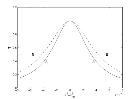
Figure 5: Transition coefficient for $\varepsilon=0.2$: asymptotic description $T_{a}(k^{2}-k^{2}_{res,a})$ (solid curve) and numerical description $T_{n}(k^{2}-k^{2}_{res,n})$ (dashed curve) for transition coefficient $T(k^{2}-k^{2}_{res})$. The width of resonant peak at height $h$: asymptotic $\Delta_{a}(h,\varepsilon)=AA$; numerical $\Delta_{n}(h,\varepsilon)=BB$.

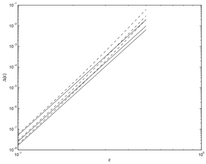
Figure 6: The width $\Delta(h,\varepsilon)$ of resonant peak for various $h$ (dashed line for numerical description, solid line for asymptotic description): line 1 for $h=0.2$; line 2 for $h=0.5$; line 3 for $h=0.7$.

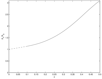
Figure 7: Ratio $\Delta_{n}(h,\varepsilon)/\Delta_{a}(h,\varepsilon)$ as function in $\varepsilon$. The ratio is independent of $h$ within the accuracy of the analysis.

The difference between the asymptotic and numerical values is more significant for larger $\varepsilon$ because the asymptotics becomes not reliable. However, as the numerical method shows, for $\varepsilon\geq 0.5$ the resonant peak turns out to be so wide that the resonant tunneling phenomenon dies out by itself.

The forms of ”asymptotic”  and ”numerical”  resonant peaks are almost the same (see Fig. 5). The difference between the peaks is quantitatively depicted in Fig. 6. Moreover, it turns out that the ratio of the width $\Delta_{n}(h,\varepsilon)$ of numerical peak at height $h$ to $\Delta_{a}(h,\varepsilon)$ of asymptotic peak is independent of $h$. The ratio as function in $\varepsilon$ is displayed in Fig. 7.

Note that for $\varepsilon=0.1$, i.e., at the left end of the band where the numerical and asymptotic results can be compared, the disparity of the results is more significant for the width of resonant peak than that for the resonant energy.

References

- [1] L. Baskin, P. Neittaanmäki, B. Plamenevskii, and O. Sarafanov, Asymptotic Theory of Resonant Tunneling in 3D Quantum Waveguides of Variable Cross-Section, SIAM J. Appl. Math., 70(2009), no. 5, pp. 1542–1566.
- [2] V.G.Maz’ya, S.A.Nazarov, and B.A.Plamenevskii, Asymptotic Theory of Elliptic Boundary Value Problems in Singularly Perturbed Domains, vol.1, 2, Birkhäser-Verlag, Basel, 2000.
- [3] V.A.Kozlov, V.G.Maz’ya, and A.Movchan, Asymptotic Analysis of Fields in Multi-Structures, Clarendon Press, New York, 1999.
- [4] B. A. Plamenevskii, O. V. Sarafanov, On a method for computing waveguide scattering matrices, St.Petersburg Math. J., 23 (2012), no.1.