Vortex liquids and the Ginzburg-Landau equation

Abstract.

We establish vortex dynamics for the time-dependent Ginzburg-Landau equation for asymptotically large numbers of vortices for the problem without a gauge field and either Dirichlet or Neumann boundary conditions. As our main tool, we establish quantitative bounds on several fundamental quantities, including the kinetic energy, that lead to explicit convergence rates. For dilute vortex liquids we prove that sequences of solutions converge to the hydrodynamic limit.

1. Introduction

Let $u:[0,\infty)\times\Omega\to\mathbb{C}$ satisfy the scaled Ginzburg-Landau equation

(1.1) $${1\over\left|\log\varepsilon\right|}\partial_{t}u=\Delta u+{1\over\varepsilon^{2}}u\left(1-|u|^{2}\right)$$

with either Dirichlet boundary conditions

(1.2) $$u =e^{in\theta+i\varphi_{\star}}\hbox{ on }\partial\Omega$$

with $\varphi_{\star}\in C^{2}$, $\int_{\partial\Omega}\partial_{\tau}\varphi_{\star}=0$, so $\deg(u;\partial\Omega)=n$, or Neumann boundary conditions

(1.3) $$\partial_{\nu}u =0\hbox{ on }\partial\Omega.$$

We take $\Omega$ to be a smooth, simply connected domain in $\mathbb{R}^{2}$ containing the origin. Equation (1.1) models the dynamic behavior of superconductors when the electromagnetic field potential is absent. When a gauge field is present, the corresponding Gorkov-Eliashberg equations

(1.4) $$\begin{split}\partial_{\Phi}u&=\nabla_{A}^{2}u+{1\over\varepsilon^{2}}u\left(1-|u|^{2}\right)\\ E&=-\operatorname{curl}\operatorname{curl}A+j_{A}(u),\end{split}$$

where $\partial_{\Phi}=\partial_{t}+i\Phi$, $E=\partial_{t}A+\nabla\Phi$, and $j_{A}(u)=\left(iu,\nabla_{A}u\right)$, provide a more complete model of superconductivity.

In order to describe the behavior of solutions of (1.1) with small $\varepsilon$ we define some fundamental quantities including:

energy density $$e_{\varepsilon}(u)={1\over 2}\left|\nabla u\right|^{2}+{1\over 4\varepsilon^{2}}\left(1-|u|^{2}\right)^{2}$$

supercurrent $$j(u)=\left(iu,\nabla u\right)$$

vorticity/Jacobian $$J(u)=\det\nabla u={1\over 2}\operatorname{curl}j(u).$$

Here $(\cdot,\cdot)$ denotes the real scalar product of two complex numbers, so $(a,b)=\frac{1}{2}(\bar{a}b+a\bar{b})$ for $a,b\in\mathbb{C}$. Solutions to equation (1.1) diffuse the Ginzburg-Landau energy

(1.5) $$E_{\varepsilon}(u)=\int_{\Omega}e_{\varepsilon}(u)$$

via the identity

(1.6) $$E_{\varepsilon}(u(t))+\int_{0}^{t}\int_{\Omega}{\left|\partial_{t}u\right|^{2}\over\left|\log\varepsilon\right|}=E_{\varepsilon}(u(0)).$$

1.1. Vortex dynamics and vortex liquids

A prominent feature of type II superconductivity is the presence of localized regions, called vortices, where superconductivity vanishes. In particular there exist some points $\{a_{j}\}_{j=1}^{n}$ in $\Omega$ where $|u(a_{j})|=0$. Furthermore, about each vortex the winding number of the phase is quantized; in particular

$${1\over 2\pi}\int_{\partial B_{r}(a_{j})}\tau\cdot j(u)\approx d\in\mathbb{Z}\backslash\{0\}.$$

In the vicinity of each vortex the Ginzburg-Landau energy $E_{\varepsilon}(u)$ blows up at the rate $\pi\left|\log\varepsilon\right|+O(1)$. Bethuel-Brezis-Hélein showed in [3] that minimizers of the Ginzburg-Landau energy (1.5) can be expanded further up to second order

(1.7) $$E_{\varepsilon}(u)=n\left(\pi\left|\log\varepsilon\right|+\gamma\right)+W(a)+o(1),$$

where $\gamma$ is a universal constant and

(1.8) $$W(a)=-\pi\sum_{i\neq j}\log|a_{i}-a_{j}|+\hbox{ boundary effects}$$

is a renormalized energy and the winding number about each vortex is one. We use the shorthand $a=(a_{1},...,a_{n})\in\Omega^{n}$ for a collection of $n$ points in $\Omega$ here.

This renormalized energy is precisely the bounded domain version of the Kirchhoff-Onsager functional that arises in two dimensional incompressible Euler equations and other settings. The renormalized energy will be discussed in more detail in Sections 2 and 3. From back-of-the-envelope calculations one finds that $J(u)$ is quantized and looks like a sum of integer-weighted delta functions; and so, for small $\varepsilon$ one finds that

$$J(u)\approx{e_{\varepsilon}(u)\over\left|\log\varepsilon\right|}\approx\pi\sum_{j=1}^{n}\delta_{a_{j}}$$

in the case when the winding number about each vortex equals one, and as $\varepsilon\to 0$, $u$ limits to

$$u_{\star}=\prod_{j=1}^{n}{x-a_{j}\over|x-a_{j}|}e^{i\psi_{\star}}$$

where $\psi_{\star}$ is $H^{1}(\Omega)$. This $u_{\star}$ is referred to as the canonical harmonic map when $\psi_{\star}$ is a harmonic function. This limiting behavior was established in many situations, see for example [3, 31, 40, 19, 20].

When dynamics (1.1) are turned on, these vortices move according to the gradient flow of the Kirchhoff-Onsager energy:

(1.9) $$\dot{a}_{j}=-{1\over\pi}\nabla_{a_{j}}W.$$

The $\left|\log\varepsilon\right|$ factor in front of (1.1) is the critical time scale on which vortices will move and can be thought of as the length of time it takes the unscaled time dependent Ginzburg-Landau equation to move an $O(\left|\log\varepsilon\right|)$ amount of energy an $O(1)$ distance. That vortices satisfy (1.9) in the limit was the subject of a formal asymptotic study by E [12]. Later, arguments of Lin [29] and Jerrard-Soner [21] provided rigorous justification of the limit. Both [29] and [21] assume that the number of vortices is uniformly bounded as $\varepsilon\to 0$. The limit equation (1.9) is the gradient flow of $W$ just as (1.1) is the (rescaled) gradient flow of the integrated energy density $\int_{\Omega}e_{\varepsilon}(u)$. The similarity in structure can also be seen by the energy dissipation identity

(1.10) $$W(a(t))+\pi\int_{0}^{t}\left|\dot{a}(s)\right|^{2}=W(a(0)).$$

This structure was exploited to give a more abstract proof of the motion law by Sandier-Serfaty [41] in their $\Gamma$-convergence of gradient flows framework.

In recent years there have been significant advances in understanding the dynamics of a finite numbers of vortices by Bethuel-Orlandi-Smets [4] on $\mathbb{R}^{2}$ and by Serfaty [46] on bounded domains. These results allow for much weaker initial conditions, handle collisions of plus/minus vortices, and describe the dynamical behavior of higher degree vortices.

On the other hand, the behavior of the time dependent Ginzburg-Landau equations with asymptotically large numbers of vortices has received mostly formal treatment. The question of how large numbers of vortices behave in superconductors is important from both experimental and numerical perspectives. In the former, typical superconductors contain many millions of vortices per sample [6, 14] so the large vortex problem is a fundamental feature of high $T_{C}$ superconducting devices. In the latter, point vortex methods provide a useful class of numerical algorithms for simulating challenging PDE’s, like vortex sheets; hence, (1.9) is a reasonable numerical approximation of the limiting mean field equation with vortex sheet initial data.

In [13] E looks at how the analogue of (1.9) on $\mathbb{R}^{2}$ behaves in a mean field sense as $n\to\infty$. Defining the vortex density function $\omega_{n}={1\over n}\sum_{j=1}^{n}\delta_{a_{j}(t)}$, the author shows that the limiting density, $\omega=\lim_{n\to\infty}\omega_{n}$, formally satisfies a weak PDE of the form

$$\partial_{{t}}\omega+\operatorname{div}(\omega v) =0$$

$$v =\nabla\left(\Delta^{-1}\right)\omega$$

after rescaling time $t$. Subsequently, this ODE limit on $\mathbb{R}^{2}$ was rigorously established by Lin-Zhang [32].

There are many similarities between this ODE limit problem and ODE limit problem arising from the point vortex method for the Euler equations. In the latter case it was shown by Schochet [44], and later by Liu-Xin [34], that the vortex density function for Euler point vortices on $\mathbb{R}^{2}$, which follow the Kirchhoff law

$$\dot{a}_{j}=-{1\over\pi}\nabla^{\perp}_{a_{j}}W(a),$$

limits to a weak Delort solution to the incompressible Euler equations on $\mathbb{R}^{2}$. Due to the similarities of the two problems, Lin-Zhang [32] used the approach of [34] to prove the associated hydrodynamic limit of the ODE (1.9) on $\mathbb{R}^{2}$.

The present work is the first to directly couple the Ginzburg-Landau equation to a mean field PDE. All previous works either prove a PDE to ODE limit for a finite number of vortices or pass from the ODE to the mean field PDE limit. Our quantitative results enable us to take the diagonal limit in a rigorous way.

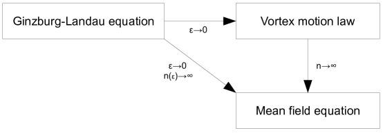
Figure 1. Limiting from the Ginzburg-Landau equation directly to the mean field equation

In order to make the direct connection between the Ginzburg-Landau equation and the limiting mean field equation, it is necessary to establish two steps. The first of which entails a proof that (1.1) can accept asymptotically large numbers of vortices for long-enough times. The second step involves coupling these Ginzburg-Landau solutions to an appropriate hydrodynamic limit of (1.9) on bounded domains.

1.2. Results

In the following we let

$$A\lesssim B\quad\hbox{ if }A\leq CB$$

for some $C$ that depends only on $\Omega$ and $\varphi_{\star}$. We tacitly assume that $\varepsilon$ is small enough that we can use estimates of the type $|\log\left|\log\varepsilon\right||\lesssim\left|\log\varepsilon\right|$.

We define the excess energy

$$D(a(t))=E_{\varepsilon}(u(t)-\left[n\left(\pi\left|\log\varepsilon\right|+\gamma\right)+W(a(t))\right],$$

where $\gamma$ and $W(a(t))$ are defined in (1.7) and (1.8); the excess energy will be used to control the deviation of the vortex path from the path defined by the ODE (1.9). We also define

$$\rho_{a}={1\over 4}\{\min_{j\neq k}\left|a_{j}-a_{k}\right|,\min_{j}\operatorname{dist}(a_{j},\partial\Omega)\}.$$

as a measure of how close vortices are to each other or the boundary. We choose a number $\rho_{\star}$ with $0<\rho_{\star}<\rho_{a(0)}$. This defines a time scale

$$\tau_{0}=\inf\left\{t>0\hbox{ such that }{\rho_{a(t)}}\leq\rho_{\star}\right\}>0$$

on which vortices will stay well-separated. For $\rho\leq\rho_{\star}$ we set

$$\Omega_{\rho}(a)=\Omega\backslash\cup_{j=1}^{n}B_{\rho}(a_{j}).$$

By $\Omega^{n*}$, we will denote the set of $a\in\Omega^{n}$ such that $a_{i}\neq a_{j}$ for $i\neq j$.

Finally, we introduce a weak topology related to the length of a minimal connection, see [5],

$$\|f\|_{\dot{W}^{-1,1}(\Omega)}=\sup_{\begin{subarray}{c}\left\|\nabla\phi\right\|_{L^{\infty}(\Omega)}\leq 1\\ \phi\in W_{0}^{1,\infty}(\Omega)\end{subarray}}\left|\int_{\Omega}\phi f\right|.$$

This norm provides a good scale-invariant measure of the distance of $J(u)$ and ${e_{\varepsilon}(u)\over\left|\log\varepsilon\right|}$ to a sum of delta functions. In particular if $|a_{j}-b_{j}|\leq\rho_{\star}$ for $j=1,\ldots,n$ then

$$\|\sum_{j}\delta_{a_{j}}-\sum_{j}\delta_{b_{j}}\|_{\dot{W}^{-1,1}(\Omega)}=\sum_{j}\left|a_{j}-b_{j}\right|.$$

We can now state our first theorem which supplies a long time existence result of the vortex motion law for asymptotically large numbers of vortices in the dilute regime.

Theorem 1.1.

Suppose $u$ solves (1.1) with either (1.2) or (1.3). Furthermore, let $n\leq{\left|\log\varepsilon\right|^{1\over 200}}$ and $\rho_{\star}\geq\left|\log\varepsilon\right|^{-{1\over 100}}$ and suppose $\|u_{\varepsilon_{n}}(0)\|_{L^{\infty}(\Omega)}\leq 1$,

(1.11) $$D(a(0)) \lesssim\left|\log\varepsilon\right|^{-{2\over 5}},$$

(1.12) $$\|J(u(0))-\pi\sum_{j=1}^{n}\delta_{a_{j}(0)}\|_{\dot{W}^{-1,1}(\Omega)} \lesssim\left|\log\varepsilon\right|^{-{1\over 3}}$$

then for all $0\leq t\leq\tau_{max}$ we have

(1.13) $$\|{e_{\varepsilon}(u)(t)\over\left|\log\varepsilon\right|}-\sum_{j=1}^{n}\pi\delta_{a_{j}(t)}\|_{\dot{W}^{-1,1}(\Omega)} \lesssim\left|\log\varepsilon\right|^{-{1\over 4}},$$

(1.14) $$\|J(u)(t)-\sum_{j=1}^{n}\pi\delta_{a_{j}(t)}\|_{\dot{W}^{-1,1}(\Omega)} \lesssim\left|\log\varepsilon\right|^{-{1\over 4}},$$

(1.15) $$\int_{\Omega_{\rho_{\star}}(a(t))}e_{\varepsilon}(|u(t)|)+{1\over 4}\left|{j(u(t))\over|u(t)|}-j(u_{\star}(t))\right|^{2} \lesssim\left|\log\varepsilon\right|^{-{1\over 5}},$$

(1.16) $$\|{j(u(t))\over|u(t)|}-j(u_{\star}(t))\|_{L^{4\over 3}(\Omega)} \lesssim\left|\log\varepsilon\right|^{-{1\over 10}}$$

where $j(u_{\star}(t))=j(u_{\star}(a(t)))$,

$$\tau_{max}=\min\left\{\tau_{0},C\sqrt{|\log\left|\log\varepsilon\right||{\rho_{\star}^{4}\over n^{3}}}\right\},$$

$a_{j}(t)$ solve (1.9), and $C=C(\Omega)$.

Theorem 1.1 can be extended to initial data having vortex degrees $d_{j}=\pm 1$ following the the approach in [23]. We also note from Lemma 14 of [23] one can easily construct maps $u_{\star}^{\varepsilon}(x;a)$ that satisfy the well-preparedness assumptions (1.11)–(1.12). Finally, in the case of a bounded number of vortices it is well known that the well-preparedness hypothesis is not very important, since one can show that data will become well-prepared almost instantaneously due to strong convergence estimates, see [29, 21, 4, 46], and we have no reason to expect a different behavior here.

Given the result above, we can prove that the sequence of solutions converge in a prescribed sense to the expected hydrodynamic limit. In this theorem we study only Dirichlet boundary conditions (1.2) since we need to have the vortex motion law hold for times of order $O(n^{-1})$, and in the Neumann case (1.3) vortices will migrate to the boundary too quickly.

What type of equations do we expect the vortex density to satisfy in the limit? Following E’s formal calculations [13] and adapting them to the bounded domain case with Dirichlet boundary conditions, we rescale time $\overline{t}={nt}$ and consider the limiting vortex density function $\omega=\lim_{n\to\infty}{1\over n}\sum_{j=1}^{n}\delta_{a_{j}(\overline{t})}$. We obtain the system

(1.17) $$\begin{split}\partial_{\overline{t}}\omega+\operatorname{div}(\omega v)&=0\\ v&=4\pi\nabla\left(\Delta^{-1}_{\mathcal{N}}\right)\omega\end{split}$$

where $\Delta^{-1}_{\mathcal{N}}:g\to w$ arises through the Poisson problem

(1.18) $$\begin{split}\Delta w&=g\hbox{ in }\Omega\\ \partial_{\nu}w&=\frac{1}{2\pi}\partial_{\tau}\theta\hbox{ on }\partial\Omega,\end{split}$$

and $\theta=\arg(x+iy)$. Note consistency requires $\int_{\Omega}g=1$ due to the Neumann boundary condition. To motivate a notion of an interior weak solution of (1.17) we follow Lin-Zhang [32]. If $\omega$ is a smooth solution to (1.17), we multiply by $\chi\in C_{0}^{\infty}([0,T]\times\Omega)$ and integrate by parts. Then, writing $t$ for $\overline{t}$ again,

$$-\int\int\partial_{t}\chi\omega-\frac{1}{4\pi}\int\int\partial_{x_{k}}\chi v_{k}\partial_{x_{j}}v_{j}=0,$$

where we used $\omega=\frac{1}{4\pi}\operatorname{div}v$ in the interior of $\Omega$. Performing integration by parts and using $\partial_{x_{1}}v_{2}-\partial_{x_{2}}v_{1}=0$, we obtain the identity

(1.19) $$\int\partial_{x_{k}}\chi v_{k}\partial_{x_{j}}v_{j}=-\int(\partial_{x_{1}}^{2}-\partial_{x_{2}}^{2})\chi(v_{1}^{2}-v_{2}^{2})-4\int\partial_{x_{1}x_{2}}\chi v_{1}v_{2},$$

and so we arrive at (1.20) below. We note that this definition is similar to the one introduced in [9, 36] for weak solutions to the 2D incompressible Euler equations except that the associated test functions are exchanged.

Definition 1.2.

We say $\omega$ is a generalized interior weak solution to (1.17) if for all $\chi\in C_{0}^{\infty}([0,T]\times\Omega)$

(1.20) $$-\int_{0}^{t}\int_{\Omega}\omega\partial_{t}\chi+\frac{1}{4\pi}\int_{0}^{t}\int_{\Omega}\left({\partial^{2}_{x_{1}}\chi-\partial^{2}_{x_{2}}\chi}\right)\left(v_{1}^{2}-v_{2}^{2}\right)+\frac{1}{\pi}\int_{0}^{t}\int_{\Omega}\partial_{x_{1}}\partial_{x_{2}}\chi\ v_{1}v_{2}=0$$

where

$$v_{j}(x)=4\pi\partial_{x_{j}}\Delta^{-1}_{\mathcal{N}}\omega=2\int\partial_{x_{j}}N(x,y)\omega(y)dy.$$

Here $N(x,y)$ is the Neumann function, which satisfies

$$\Delta N(\cdot,y) =2\pi\delta_{y}\quad\text{in $\Omega$}$$

$$\partial_{\nu}N(\cdot,y) =\partial_{\tau}\theta\quad\text{on $\partial\Omega$}.$$

We can now state our main result which shows that we can solve (1.17)-(1.18) with vortex sheet initial data via a subsequence of either solutions of (1.1) or (1.9) with appropriate data.

Theorem 1.3.

Assume that $\omega_{0}\in\mathcal{M}\cap\dot{H}^{-1}(\Omega)$ satisfies $\omega_{0}\geq 0$, $\int_{\Omega}\omega_{0}=1$, and $\operatorname{supp}(\omega_{0})\subset\{\operatorname{dist}(x,\partial\Omega)\geq C_{0}>0\}$ for some constant $C_{0}$. Then there exists a sequence of initial data $u_{\varepsilon_{n}}(0)$ with $n=|\log|\log|\log\varepsilon_{n}|||^{1\over 4}$ number of vortices that satisfies the hypotheses for Theorem 1.1 such that ${1\over n}{e_{\varepsilon_{n}}(u_{\varepsilon_{n}}(0))\over\pi|\log\varepsilon_{n}|}\to\omega_{0}$ in $\mathcal{M}$ as $\varepsilon_{n}\to 0$. Such initial data generates a sequence of solutions $u_{\varepsilon_{n}}(t)$ of (1.1) with boundary condition (1.2) for times up to $T=|\log|\log\varepsilon_{n}||^{1\over 7}$.

Setting $\overline{t}=nt$ and letting $\omega_{\varepsilon_{n}}(\overline{t})={1\over n}{e_{\varepsilon_{n}}(u_{\varepsilon_{n}}(\overline{t}))\over\pi|\log\varepsilon_{n}|}$ then for a subsequence

$$\omega_{\varepsilon_{n}}\to\omega\hbox{ in }\mathcal{M}(\Omega\times[0,\infty))$$

where $\omega$ is a generalized interior weak solution, defined above, to

(1.21) $$\begin{split}\partial_{\overline{t}}\omega+\operatorname{div}\left(v\omega\right)&=0\\ v&=4\pi\nabla\left(\Delta^{-1}_{\mathcal{N}}\right)\omega\end{split}$$

Finally, $v(\overline{t})\in L^{2}_{loc}(\Omega)$. Here $\Delta^{-1}_{\mathcal{N}}f=w$ if

(1.22) $$\begin{split}\Delta w&=f\hbox{ in }\Omega\\ \partial_{\nu}w&=\frac{1}{2\pi}\partial_{\tau}\theta\hbox{ on }\partial\Omega\end{split}$$

where $\theta=\arg(x+iy)$ and $\int_{\Omega}f=1$.

The convergence to the hydrodynamic limit holds true for a more general class of initial data similar to those we construct in Theorem 1.3. This yields the following result on the limit from the parabolic Ginzburg-Landau equation to the mean field equation:

Theorem 1.4.

Let $u_{\varepsilon_{n}}(0)$ be a sequence of initial data to the Ginzburg-Landau equation (1.1) with Dirichlet boundary conditions (1.2) with $||u_{\varepsilon_{n}}(0)||_{L^{\infty}(\Omega)}\leq 1$ and satisfies the following hypotheses:

(1.23) $$\left\|J(u_{\varepsilon_{n}}(0))-\sum_{j=1}^{n}\pi\delta_{a_{j}(0)}\right\|_{\dot{W}^{-1,1}(\Omega)} \lesssim\left|\log\varepsilon_{n}\right|^{-{1\over 3}}$$

(1.24) $$D(a(0)) \lesssim\left|\log\varepsilon_{n}\right|^{-{2\over 5}}$$

(1.25) $$n \leq\left|\log|\log\left|\log\varepsilon_{n}\right||\right|^{1\over 4}$$

with $a(0)\in\Omega^{n}$ satisfying the following:

(1.26) $$\rho_{a(0)} \geq\left|\log|\log\left|\log\varepsilon_{n}\right||\right|^{-{1\over 3}}$$

(1.27) $$-{1\over n^{2}}\sum_{j\neq k}N_{n}(a_{j}(0),a_{k}(0)) \lesssim 1,$$

where $N_{n}(\cdot,\cdot)$ is defined in Section 3 and is closely related to $N(\cdot,\cdot)$. Setting $\overline{t}=nt$ and letting $\omega_{\varepsilon_{n}}(\overline{t})={1\over n}{e_{\varepsilon_{n}}(u_{\varepsilon_{n}}(\overline{t}))\over\pi|\log\varepsilon_{n}|}$ then for a subsequence

$$\omega_{\varepsilon_{n}}\to\omega\hbox{ in }\mathcal{M}(\Omega\times[0,\infty)).$$

where $\omega(\overline{t})$ is a generalized interior weak solution to (1.21) for $\overline{t}\in(0,\infty)$. If $v=4\pi\nabla\left(\Delta^{-1}_{\mathcal{N}}\right)\omega$, defined by $\eqref{definitionNeumannLaplaceOp}$, then $v(\overline{t})\in L^{2}_{loc}(\Omega)$.

The assumptions of Theorem 1.4 may look rather demanding; nevertheless, such data exist per the construction in the proof of Theorem 1.3. Furthermore, we expect that fairly generic data corresponding to a collection of degree $1$ vortices will satisfy such assumptions after a short time since the parabolic Ginzburg-Landau equation quickly dissipates not only the Ginzburg-Landau energy and the renormalized energy, but also the excess energy, compare [4, 46].

1.3. Discussion

The issue of whether the weak solution satisfies the correct boundary condition is a deep and difficult question. Since vorticity can (and should) concentrate on the boundary, it is difficult to acquire the necessary regularity to ensure the boundary conditions are achieved in the classical weak sense. Some recent progress has been made in [17] by establishing boundary-coupled weak solutions of the two dimensional incompressible Euler equations in exterior domains.

To make a fully consistent limit it would be interesting to study the question of uniqueness of the limiting mean field equation (1.21). In [32] the authors establish uniqueness for initial data in $L^{\infty}$ with compact support for the problem in $\mathbb{R}^{2}$. A similar study of regular solutions would be natural for (1.21)-(1.22) too.

From formal considerations of (1.21) the vortex density function satisfies $\partial_{t}\omega+v\cdot\nabla\omega=-4\pi\omega^{2}$, so along the trajectory of the induced velocity one sees that the density function should decay like $t^{-1}$. For smooth initial data on $\mathbb{R}^{2}$ Lin-Zhang [32] proved this fact, which implies that the vorticity spreads out quickly from a compact set. This behavior implies that we expect most vortices to be pushed out to the boundary in a similar fashion. This conforms to the picture presented in Sandier-Soret [43] for global minimizers of the functional $E_{\varepsilon}(u)$ on bounded domains, constrained to the boundary condition of the type $u=e^{in\theta}$ and $n\to\infty$. Sandier-Soret show that vortices accumulate close to the boundary of the domain as $n$ grows asymptotically large. Taken together, we should view Theorem 1.3 as a mean field description of the vortex density for times in the mesoscale in the interior of the domain.

The dilute density of the vortex liquid results from two issues. The first is that we use energy comparison and a Gronwall inequality to pin the vortex positions to the ODE (1.9). This results in an upper bound $\tau_{max}\lesssim\sqrt{{\rho_{\star}^{4}\over n^{3}}|\log\left|\log\varepsilon\right||}$ in Theorem 1.1. Integrating methods of [46] and/or [4] should improve some of these bounds. The second issue arises from the poor bounds on the intervortex distance for the ODE (1.9). Better knowledge of how the ODE behaves should improve the vortex density allowed here.

Although (1.1) provides a fertile ground to test the mathematics of the Gorkov-Eliashberg equations, the more physical problem entails looking at the hydrodynamic limit of (1.4). For the Gorkov-Eliashberg equations (1.4), corresponding proofs of the vortex motion law are due to the second author [49] for $O(1)$ fields and Sandier-Serfaty [41] for larger fields, following the formal asymptotic work of [38]. Formally, it was shown by Chapman-Rubinstein-Schatzman [7] that the hydrodynamic limit of the associated ODE arising from the vortex motion law of (1.4) converges to a weak solution of

(1.28) $$\begin{split}\partial_{{t}}\omega+\operatorname{div}(\omega v)&=0\\ v&=\nabla\left(\Delta-\mathbb{I}\right)^{-1}\omega.\end{split}$$

There has been a lot of recent progress on the limiting equations for the vortex densities (1.28). Ambrosio-Serfaty [1] and Ambrosio-Mainini-Serfaty [2] study them as a metric gradient flow in the space of measures, with the Wasserstein distance as the natural metric. However, they do not obtain the convergence. Even when it becomes possible to carry out the program outlined in the survey of Serfaty [47] and to directly obtain the Wasserstein gradient flow studied in [1, 2] from the Gorkov-Eliashberg equation by a $\Gamma$-convergence of gradient flows type result, we believe that our approach will still be useful. For one, it provides quantitative bounds that are useful in type II superconductors without going to the $\varepsilon\to 0$ limit of “extreme” type II superconductivity. More importantly, as our approach does not rely on the gradient flow structure, it can be adapted to yield results for more general situations, such as the mixed flows studied in [26] and [37] for the ungauged problem and in [27] and [48] for the gauged problem. Such motion laws have physical importance, as they can be used to explain the sign-change in the Hall effect of type II superconductors, see [11], [24]. Similarly, we expect that our approach can be adapted also to the Hamiltonian Ginzburg-Landau wave system, where results for the PDE to ODE limit for finitely many vortices have been found in [18] and [30], and the ODE to mean field PDE limit has been studied in [33].

1.4. Method

We finish the introduction with an outline of the arguments in the paper. The general scheme of the paper is to deduce the vortex motion law for the time dependent Ginzburg-Landau equations by carefully considering certain differential identities, in particular the time evolution of the energy density.

Our proof is based on the following differential identities, which hold for smooth solutions of (1.1):

(1.29) mass identity $$\left[{1\over\left|\log\varepsilon\right|}\partial_{t}-\Delta-{2\over\varepsilon^{2}}|u|^{2}\right]\left(|u|^{2}-1\right)=2\left|\nabla u\right|^{2}$$

(1.30) supercurrent identity $${1\over\left|\log\varepsilon\right|}\left(iu,\partial_{t}u\right)=\text{div}j(u)$$

(1.31) energy identity $$\partial_{t}e_{\varepsilon}(u)=\text{div}\left(\partial_{t}u,\nabla u\right)-{\left|\partial_{t}u\right|^{2}\over\left|\log\varepsilon\right|}.$$

For fixed $\varepsilon$ regularity follows from standard parabolic theory. We remark that (1.29) can be used to show that $0\leq|u|\leq 1$; (1.30) will be used to show that $j(u)$ is nearly divergence-free in a time-averaged sense.

The identity (1.31) is crucial in obtaining a lower bound for the kinetic energy. Using (1.1) once more, we can also deduce from (1.31)

(1.32) $$\frac{1}{\left|\log\varepsilon\right|}\partial_{t}e_{\varepsilon}(u)=\mathrm{div}\ \mathrm{div}\left(\nabla u\otimes\nabla u-\frac{1}{2}e_{\varepsilon}(u)\mathrm{id}\right)-\frac{|\partial_{t}u|^{2}}{\left|\log\varepsilon\right|^{2}},$$

which is the primary tool to establish the vortex motion law.

Passing to the limit $\varepsilon\to 0$ in (1.32) and controlling the growth of the energy excess would yield a proof of the motion law for bounded numbers of vortices if the initial energy excess is $o(1)$ as $\varepsilon\to 0$. This method is not as powerful as the elliptic PDE approach of Serfaty [45, 46] or the parabolic PDE approach of Bethuel-Orlandi-Smets [4], but it provides a way to avoid using convergence properties in the proof, and we can use quantitative estimates in every step. Passing to the limit $\varepsilon\to 0$ for bounded $n$, our results are weaker than those in the literature, but our explicit bounds provide rates of convergence.

Our approach of using differential identities and explicit estimates follows the program of the second author and R. Jerrard [23] for the Gross-Pitaevsky equation $i\partial_{t}u=\Delta u+{1\over\varepsilon^{2}}u\left(1-|u|^{2}\right)$. Surprisingly, implementing this approach for (1.1) is more challenging and requires several new estimates.

One such additional difficulty is that the arguments of all previous vortex motion law proofs for (1.1) use a limiting kinetic energy lower bound, which has so far only been available for a bounded number of vortices. In Theorem 5.1, one of our central results, we provide such a bound for a large number of vortices. This type of estimate is not needed for the Gross-Pitaevsky equation since one has conservation of energy for both the PDE and ODE in that case.

We give an overview of the contents of the rest of the paper.

In Section 2, we recall some known results on the renormalized energy. Lemma 2.1 connects the gradient of the renormalized energy to the canonical harmonic map $u_{\star}$, and Proposition 2.3 quantifies how close $u$ and $u_{\star}$ are based on the excess energy.

In Section 3, we give some detailed results for the renormalized energy in the Dirichlet case, following Sandier-Soret [43]. These estimates are used to show that vortices stay away both from each other and the boundary for sufficiently long times to pass to the hydrodynamic limit under certain conditions.

In Section 4, we discuss localization estimates for the Jacobian and energy density. For the Jacobian, results of [23] yield points $\xi_{j}$ such that $\|J(u)-\pi\sum\delta_{\xi_{j}}\|_{{{\dot{W}}^{-1,1}}}$ is small in a precisely quantified way. We provide a new estimate on the localization of the Ginzburg-Landau energy density to the same set of delta functions of the type

$$\left\|{e_{\varepsilon}(u)\over\left|\log\varepsilon\right|}-\sum_{j=1}^{n}\pi\delta_{\xi_{j}}\right\|_{\dot{W}^{-1,1}(\Omega)}\lesssim{1\over\left|\log\varepsilon\right|}\left[W(a)+nD(a)\right].$$

The estimate presented here is a refined (i.e. $\varepsilon$-rate dependent) version of an estimate found in Colliander-Jerrard [8]. Therefore, in order to localize the vortices to a high resolution, we need good estimates on the excess energy, $D(a(t))$.

Since the localization and gamma stability error estimates depend explicitly on the excess energy, it is necessary to understand how the excess energy evolves in time. By the energy dissipation identities (1.6) and (1.10) we see that

(1.33) $$D(a(t))=D(a(0))+\pi\int_{0}^{t}{\left|\dot{a}\right|^{2}}-\int_{0}^{t}\int_{\Omega}{\left|\partial_{t}u\right|^{2}\over\left|\log\varepsilon\right|};$$

consequently, $D(a(t))$ can be controlled by well-preparedness of the initial data and a lower bound on the kinetic energy. This lower bound is presented in Section 5 as Theorem 5.1:

$$\int_{0}^{t}\int_{\Omega}{\left|\partial_{t}u\right|^{2}\over\left|\log\varepsilon\right|}-\pi\int_{0}^{t}{\left|\dot{a}\right|^{2}}\geq-\mathbf{error},$$

where $\mathbf{error}$ depends explicitly on $\varepsilon$, the number of vortices, the minimal vortex distance, the time scale and the localization error. This result provides a purely quantitative approach to the kinetic energy lower bounds that are found in [30, 18, 41], each of which rely on compactness properties to get a lower bound. To establish this result we make quantitative the kinetic energy estimate of [30], who used the differential identity for the energy density, along with a limiting result on the equipartitioning of potential energy. Here we make use of an optimal quantitative equipartitioning result in [28] that identifies how close in $L^{1}$ the tensor $\nabla u\otimes\nabla u$ is to the diagonal matrix $\frac{1}{2}|\nabla u|^{2}\mathrm{id}$. Placing this equipartitioning result into the differential identity for the Ginzburg-Landau energy $e_{\varepsilon}(u)$, applying a test function

$$\sum\chi(x-a_{j}(t))\dot{a}_{j}(t)\cdot(x-a_{j}(t)),\ \hbox{ $\chi$ a smooth cutoff function},$$

and integrating over $\Omega$ yields the lower bound.

After these preparations, we prove Theorem 1.1 in Section 6. The main task is to understand how close the points $\xi_{j}(t)$, found by the localization estimates, are to the points $a_{j}(t)$ given by the ODE. To this end, we introduce a quantity $\eta(t)$ which serves as a differentiable replacement for $\pi\sum_{j}|\xi_{j}(t)-a_{j}(t)|$.

In Subsection 6.1, we define various small quantities that serve as error bounds in our estimates, and several time intervals on which good estimates hold; in particular, we show that $\eta$ really controls everything we need.

It therefore suffices to control the growth of $\eta$ via a Gronwall argument. We estimate $\dot{\eta}$ in Subsection 6.2, relying on the energy evolution (1.32). The resulting simple bound of the type $|\dot{\eta}|\lesssim A_{\varepsilon}\sqrt{\eta}+o(1)_{\varepsilon}$ is not sufficient to apply the Gronwall inequality globally, but yields a reasonable short time result. The culprit for the $\sqrt{\eta}$ is a certain supercurrent estimate that is difficult to improve at a fixed time.

Subsection 6.3 provides the necessary improvements by averaging over a short timescale, $\dot{\left<\eta\right>}\lesssim\widetilde{A}_{\varepsilon}\left<\eta\right>+o(1)_{\varepsilon}$. This technique, taken from [23], makes use of (1.30) to obtain a quantitative bound on how far $j(u)$ is from being divergence free. Using a Hodge decomposition of $\frac{j(u)}{|u|}-j(u_{\star})$ and the fact that $j(u_{\star})$ is divergence free while $\operatorname{curl}(j(u)-j(u_{\star})$ is controlled, we can bound time averages of terms of the type $\int_{\Omega_{\rho}}\zeta\left({j(u)\over|u|}-j(u_{\star})\right)$ for some prescribed function $\zeta$. As in [23], this part is fairly technical, but the differences from the Gross-Pitaevsky case are significant enough that we feel it is necessary to include these details.

The proof of Theorem 1.1 is finished in Subsection 6.4, where we show via a continuity argument that $J(u)$ is localized near the $a(t)$ for long times. In particular, we obtain the vortex motion law.

In the final Section 7, we consider the hydrodynamic limit and prove Theorems 1.3 and 1.4. In the first part of the section, we prove a hydrodynamic limit of the vortex ODE’s for bounded domains which is analogous to the results of [44, 34] for the Euler point vortex method on $\mathbb{R}^{2}$ and the gradient flow version of [32] on $\mathbb{R}^{2}$ for bounded domains. The proof requires a careful expansion of the time dependent behavior of ${1\over n}\sum_{j=1}^{n}\delta_{a_{j}(t)}$ integrated against a test function with compact support. Implementing the strategy of [34, 32] and using estimates on the Neumann function, we prove the convergence and the local velocity bound.

To complete the proof of Theorem 1.3, we show that nonnegative vortex sheet initial data with compact support can be approximated by a sequence of a sum of degree-one vortices that satisfy the conditions of our class of initial data. This improves on the construction in [32], which uses vortex blobs with arbitrary vorticities. Finally, due to Theorem 1.1, the quantity $\omega_{n}(t)={1\over n}{e_{\varepsilon}(u(t))\over\pi\left|\log\varepsilon\right|}$ converges to the same limit as the vortex density function ${1\over n}\sum_{j=1}^{n}\delta_{a_{j}(t)}$.

2. The renormalized energy

In this section we recall some results on the renormalized energy and the canonical harmonic map.

Recall from [3] the canonical harmonic map $u_{\star}={u_{\star}(\alpha)}$ which satisfies the following Hodge system

$${\operatorname{div}j(u_{\star})=0\qquad\operatorname{curl}j(u_{\star})=2\pi\sum_{j=1}^{n}\delta_{\alpha_{j}}}$$

with either

$$j(u_{\star})\cdot\tau=n\partial_{\tau}\theta+{\partial_{\tau}\varphi_{\star}}$$

on $\partial\Omega$ or

$$j(u_{\star})\cdot\nu=0$$

on $\partial\Omega$. There exists a $G$ with $\nabla^{\perp}G=j(u_{\star})$, where $G(x)=G(x;\alpha)$ is defined by the following Poisson equation

(2.1) $$\Delta G=2\pi\sum_{j=1}^{n}\delta_{\alpha_{j}}\hbox{ in }\Omega$$

with either

$$\partial_{\nu}G=n\partial_{\tau}\theta+{\partial_{\tau}\varphi_{\star}}\hbox{ on }\partial\Omega$$

or

$$G=0\hbox{ on }\partial\Omega.$$

The renormalized energy is then defined, recalling $\Omega_{\rho}(\alpha)=\Omega\setminus\cup_{j=1}^{n}B_{\rho}(\alpha_{j})$, as

$${W(\alpha)}=\lim_{\rho\to 0}\left(\int_{\Omega_{\rho}(\alpha)}{1\over 2}\left|\nabla u_{\star}\right|^{2}-\pi n\log{1\over\rho}\right).$$

We also define the approximate energy as

$${W_{\varepsilon}(\alpha)=W(\alpha)}+n\left(\pi\left|\log\varepsilon\right|+\gamma\right)$$

where

$$\gamma=\lim_{\varepsilon\to 0}\left(\inf_{u\in H^{1}(B_{1};\mathbb{C}),u(z)=z\text{ on $\partial B_{1}$}}E_{\varepsilon}(u)-\pi\left|\log\varepsilon\right|\right)$$

is the constant from [3, Lemma IX.1]. Finally, the excess energy is defined as

(2.2) $${D(u;\alpha)=E_{\varepsilon}(u)-W_{\varepsilon}(\alpha).}$$

We usually simplify this to $D(\alpha)$ when the context is unambiguous.

We also define the excess energy in the ball $B_{\sigma}(\alpha_{j})$ to be

$$D_{B_{\sigma}(\alpha_{j})}=\int_{B_{\sigma}(\alpha_{j})}e_{\varepsilon}(u)-\left(\pi\log{\sigma\over\varepsilon}+\gamma\right).$$

We will use the following characterization of the gradient of the renormalized energy.

Lemma 2.1 (Lin [29], Jerrard-Soner [21], Jerrard [18]).

Let $\alpha\in\Omega^{n*}$ then the canonical harmonic map $u_{\star}=u_{\star}(\cdot;\alpha)$ and the renormalized energy $W(\alpha)$ satisfy

$$\int\partial_{x_{k}x_{m}}\zeta\left[\left(j(u_{\star})\right)_{m}\left(j(u_{\star})\right)_{k}-{1\over 2}\delta_{km}\left|j(u_{\star})\right|^{2}\right]=-\sum_{j=1}^{n}\partial_{k}\zeta(\alpha_{j})\left(\nabla_{\alpha_{j}}W(\alpha)\right)_{k}$$

where $\zeta\in C^{2}(\Omega)$ and $\nabla^{2}\zeta$ has support in an annular neighborhood of the $\alpha_{j}$’s.

Next we list estimates on the canonical harmonic map and renormalized energy and their derivatives.

Lemma 2.2.

There exists a constant $C$ depending only on $\Omega$ such that for every bounded, open $\Omega\subset\mathbb{R}^{2}$, $\alpha\in\Omega^{n*}$, the renormalized energy $W(\alpha)$, canonical harmonic map $u_{\star}(\cdot,;\alpha)$ and its potential $G(\cdot;\alpha)$ as defined in (2.1) satisfy

(2.3) $$\|j(u_{\star})\|_{L^{\infty}(\Omega_{r}(\alpha))}\ =\ \|\nabla G\|_{L^{\infty}(\Omega_{r}(\alpha))}\ \leq\ \frac{2n}{r}$$

for all $r\leq\rho_{\alpha}$, and

(2.4) $$|\nabla_{i}W(\alpha)|\leq\frac{Cn}{\rho_{\alpha}},\quad\quad|\nabla_{i}\nabla_{j}W(\alpha)|\leq\frac{Cn}{\rho_{\alpha}^{2}}$$

for every $i,j\in\{1,\ldots,n\}$.

We also have the upper bound

(2.5) $$W(\alpha)\leq C(n^{3}+\frac{n^{2}}{\rho^{2}_{\alpha}}).$$

Finally, let $\alpha=(\alpha_{1},\ldots,\alpha_{n})$ and $\alpha^{\prime}=(\alpha_{1}^{\prime},\ldots,\alpha_{n}^{\prime})$ with $\alpha,\alpha^{\prime}\in\Omega^{n*}$. Let $\Omega_{r}(\alpha,\alpha^{\prime})=\Omega\backslash\left(\cup_{j=1}^{n}B_{r}(\alpha_{j})\cup B_{r}(\alpha_{j}^{\prime})\right)$, then

(2.6) $$\left\|j(u_{\star})(\alpha)-j(u_{\star})(\alpha^{\prime})\right\|_{L^{\infty}(\Omega_{r}(\alpha,\alpha^{\prime}))}\leq{1\over r^{2}}\sum_{j=1}^{n}\left|\alpha_{j}-\alpha_{j}^{\prime}\right|$$

for all $r\leq\min\{\rho_{\alpha},\rho_{\alpha^{\prime}}\}$, and additionally, for $1<p<2$,

(2.7) $$\|j(u_{\star}(\alpha))-j(u_{\star}(\alpha^{\prime}))\|_{L^{p}}\leq(\pi\sum|\alpha_{i}-\alpha_{i}^{\prime}|)^{\frac{2}{p}-1}(2n\pi)^{2-\frac{2}{p}}.$$

Proof.

The Neumann boundary condition results are proved in Lemma 10, Lemma 11, and Lemma 13 of [23]; we note a typo in the statement of estimate (2.5) in [23]. Corresponding results for the Dirichlet boundary condition can be established by using similar arguments. Further estimates in the Dirichlet case are discussed in Section 3. ∎

Finally, we will need the following quantitative coercivity or $\Gamma$-stability result for the renormalized energy:

Proposition 2.3 (Jerrard-Spirn, Theorem 2 of [23]).

Let $\Omega$ be a bounded, open simply connected subset of $\mathbb{R}^{2}$ with $C^{1}$ boundary. Then there exist constants $C$, $K_{\star}$ depending only on $\Omega$ such that for any $u\in H^{1}(\Omega;\mathbb{C})$, if there exist $n\geq 0$, finite, with $\alpha=(\alpha_{1},\ldots,\alpha_{n})\in\Omega^{n*}$ such that

$$\left\|J(u)-\sum_{j=1}^{n}\pi\delta_{\alpha_{j}}\right\|_{\dot{W}^{-1,1}}\leq s_{\varepsilon}\qquad\hbox{ for some }s_{\varepsilon}\in[\varepsilon\sqrt{\log(\rho_{\alpha}/\varepsilon)},{\rho_{\alpha}/K_{\star}}],$$

and if $4s_{\varepsilon}\leq\sigma^{*}=\sqrt{{\rho_{\alpha}\over n^{3}}\left(s_{\varepsilon}+\varepsilon E_{\varepsilon}(u)\right)}\leq{\rho_{\alpha}\over K_{\star}}$ then

(2.8) $$\int_{\Omega_{\sigma^{*}}(\alpha)}e_{\varepsilon}(|u|)+{1\over 4}\left|{j(u)\over|u|}-j(u_{\star}(\alpha))\right|^{2}\leq D(\alpha)+C\sqrt{{n^{5}\over\rho_{\alpha}}\left({s_{\varepsilon}}+{\varepsilon}E_{\varepsilon}(u)\right)}.$$

Finally,

$$\left\|j(u)-j(u_{\star}(\alpha))\right\|_{L^{4\over 3}}\leq C\sqrt{D(\alpha)}+{\mathbf{error}}$$

and

$$\mathbf{error} \leq C\varepsilon^{1\over 2}E_{\varepsilon}(u)^{3\over 4}$$

$$\quad+Cn\left(s_{\varepsilon}+\varepsilon E_{\varepsilon}(u)\right)^{1\over 4}\left[\left({n\over\rho_{\alpha}}\right)^{1\over 4}+\rho_{\alpha}^{1\over 4}\left(1+\sqrt{E_{\varepsilon}(u)\over n^{3}}\right)\right].$$

3. Estimates for the Dirichlet case

In this section we provide estimates on the Neumann functions that comprise the renormalized energy in the Dirichlet case. These estimates will be used both to generate long-lived solutions of (1.1) with asymptotically many vortices and to provide kernel estimates for the hydrodynamic limit theorem.

We follow the approach of Sandier-Soret [43] to define the renormalized energy in terms of Neumann functions. In particular let $N_{n}(x,y)$ denote the Neumann function which satisfies the following equation

$$\begin{split}\Delta N_{n}(\cdot,y)&=2\pi\delta_{y}\hbox{ in }\Omega\\ \partial_{\nu}N_{n}(\cdot,y)&=\partial_{\tau}\theta+{1\over n}\partial_{\tau}\varphi_{\star}\hbox{ on }\partial\Omega\\ \int_{\partial\Omega}N_{n}(\cdot,y)(\partial_{\tau}\theta+{1\over n}\partial_{\tau}\varphi_{\star})&=0\end{split}$$

and the limiting Neumann function $N(x,y)=N_{\infty}(x,y)$ which satisfies the following equation

$$\begin{split}\Delta N(\cdot,y)&=2\pi\delta_{y}\hbox{ in }\Omega\\ \partial_{\nu}N(\cdot,y)&=\partial_{\tau}\theta\hbox{ on }\partial\Omega\\ \int_{\partial\Omega}N(\cdot,y)\partial_{\tau}\theta&=0.\end{split}$$

We also define $H_{n}(x,y)=N_{n}(x,y)-\log|x-y|$ and $H(x,y)=N(x,y)-\log|x-y|$ to be the harmonic pieces of the Neumann functions $N_{n}(x,y)$ and $N(x,y)$, respectively. Then

(3.1) $$W(a_{1},\ldots,a_{n})=-\pi\sum_{j\neq k}N_{n}(a_{j},a_{k})-\pi\sum_{j=1}^{n}H_{n}(a_{j},a_{j}),$$

see [3, 43].

We state the following useful set of estimates:

Lemma 3.1 (Sandier-Soret [43]).

The Neumann function $N_{n}(x,y)$ satisfies for $1\leq n\leq\infty$ the estimates

1. $N_{n}(x,y)=N_{n}(y,x)$

2. $N_{n}(x,y)=\log|x-y|+H_{n}(x,y)$ where $H_{n}(x,y)$ is continuous on $\Omega\times\overline{\Omega}\cup\overline{\Omega}\times\Omega$.

3. $N_{n}(x,y)=2\log|x-y|+\widetilde{H}_{n}(x,y)$ where $\widetilde{H}_{n}$ is continuous on $\partial\Omega\times\overline{\Omega}\cup\overline{\Omega}\times\partial\Omega$.

In the proof of Lemma 3.1 the authors generate $H_{n}(x,y)$ in steps. When $\Omega=B_{1}$ and $\partial_{\nu}N(\cdot,y)=1$ then $H(x,y)=\widehat{H}(x,y)$, where $\widehat{H}$ can be explicitly computed:

(3.2) $$\widehat{H}(x,y)=\log|1-x\overline{y}|.$$

For nontrivial $\partial_{\nu}N_{n}(\cdot,y)=f_{n}=\partial_{\tau}\theta+{1\over n}\partial_{\tau}\varphi_{\star}$ one finds $\widehat{H}_{n}$ satisfies $\widehat{H}_{f_{n}}(x,y)=\widehat{H}(x,y)+P(x)+Q(y)$ where $P(x)$ and $Q(y)$ are harmonic in $B_{1}$ and bounded and continuous up to the boundary. Finally, for simply-connected domain $\Omega$ let $w(z)$ denote the conformal mapping of $\Omega$ into $B_{1}$. Then one finds

(3.3) $$H_{n}(x,y)=\widehat{H}_{\widehat{f_{n}}}(w(x),w(y))$$

where $\widehat{f_{n}}(x)$ is defined as $\widehat{f_{n}}(w(z))=f_{n}(z)/|w^{\prime}(z)|$. We note again that in our case $\widehat{f_{n}}(x)=\partial_{\tau}\theta+{1\over n}\partial_{\tau}\varphi_{\star}$.

Using (3.1) and Lemma 3.1 we prove the following lemma that provides a lower bound on the intervortex distance as a function of the renormalized energy.

Lemma 3.2.

Let $W(a)$ be the renormalized energy for the Dirichlet case, then

$$\rho_{a} \geq e^{-{\frac{1}{\pi}W(a)}-Cn^{2}}$$

for some constant $C$ that depends only on $\Omega$ and $\varphi_{\star}$.

Proof.

Since the domain is bounded we have from (2) and (3) of the Sandier-Soret lemma

$${\frac{1}{\pi}W(a)} =-\sum_{j\neq k}N_{n}(a_{j},a_{k})-\sum_{j}H_{n}(a_{j},a_{j})$$

$$\geq\log[\min\{\min_{j\neq k}\{|a_{j}-a_{k}|\},\min_{j}\{\operatorname{dist}(a_{j},\partial\Omega)\}\}]^{-1}-Cn^{2}$$

$$\geq\log\rho^{-1}_{a}-Cn^{2},$$

where $C$ depends on $\varphi_{\star}$ and $\Omega$. Therefore,

$$\rho_{a}=e^{\log\rho_{a}}\geq e^{-{\frac{1}{\pi}W(a)}-Cn^{2}}.$$

∎

The following proposition gives a class of data where a good bound on the minimal intervortex distance holds for all time.

Proposition 3.3.

Assume that $a_{j}(t)$ are solutions to

$$\dot{a}_{j}=-{1\over\pi}\nabla_{a_{j}}W(a)$$

with the renormalized energy $W$ arising from the Dirichlet boundary condition (1.2). If $\rho_{a(0)}\geq\left|\log|\log\left|\log\varepsilon\right||\right|^{-{1\over 3}}$ and $n\leq\left|\log|\log\left|\log\varepsilon\right||\right|^{1\over 4}$ then the $a_{j}(t)$ satisfy

$${\rho_{a(t)}\geq\frac{1}{C}|\log\left|\log\varepsilon\right||^{-{1\over 10}}}$$

for all $t$.

Proof.

From our assumptions on $\rho_{a(0)}$ and $n$ we have

$$W(a(0))\leq C{n^{2}\over\rho_{a(0)}}\leq C|\log|\log\left|\log\varepsilon\right|||^{5\over 6}.$$

Since $W(a(t))\leq W(a(0))$ then from Lemma 3.2 we see that

$$\rho^{-1}_{a(t)} \leq Ce^{{\frac{1}{\pi}}W(a(t))+Cn^{2}}\leq Ce^{{\frac{1}{\pi}}W(a(0))+Cn^{2}}$$

$$\leq Ce^{C|\log|\log\left|\log\varepsilon\right|||^{{5\over 6}}}\leq Ce^{{1\over 10}|\log|\log\left|\log\varepsilon\right|||}$$

for all time. ∎

We note that for this class of initial data and setting $\rho_{\star}=|\log|\left|\log\varepsilon\right|||^{-{1\over 6}}$ so $\rho_{a(t)}\geq\rho_{\star}$, the quantity $T=C\sqrt{|\log\left|\log\varepsilon\right||{\rho_{\star}^{4}\over n^{3}}}$ that appears in the assumptions of Theorem 1.1 satisfies $T\gtrsim\frac{1}{n}$, since

$$C\sqrt{|\log\left|\log\varepsilon\right||{\rho_{\star}^{4}\over n^{3}}}\geq C{|\log\left|\log\varepsilon\right||^{1\over 6}\over|\log|\log\left|\log\varepsilon\right|||^{3\over 4}}\geq|\log\left|\log\varepsilon\right||^{1\over 7}\gtrsim\frac{1}{n},$$

so the time rescaling in Theorem 1.3 makes sense.

4. Localization results

In this section we discuss quantitative estimates that show how well the fundamental quantities $J(u)$ and $\frac{e_{\varepsilon}(u)}{\left|\log\varepsilon\right|}$ are approximated by sums of point masses. For $J(u)$, these results were shown in [22, 23]; for the energy, they are new.

Proposition 4.1 (Jerrard-Spirn, Theorem 3 of [23]).

Let $\Omega$ be a bounded, open, simply connected subset of $\mathbb{R}^{2}$ with $C^{1}$ boundary. Then there exist constants $C>0$ and $C_{\star}\geq 2$, with $C_{\star}=\max\{K_{\star},{1\over 4}\operatorname{diam}(\Omega)\}$ and $K_{\star}$ is the constant from Proposition 2.3, such that the following property holds.

For any $u\in H^{1}(\Omega;\mathbb{C})$, if there exist $n\geq 0$, $\alpha=\left(\alpha_{1},\ldots,\alpha_{n}\right)\in\Omega^{n*}$ such that

$$\left\|J(u)-\sum_{j=1}^{n}\pi\delta_{\alpha_{j}}\right\|_{\dot{W}^{-1,1}}\leq\frac{\rho_{\alpha}}{8C_{\star}n^{5}},$$

and if in addition $E_{\varepsilon}(u)\geq 1$ and

(4.1) $$\left[\frac{n^{5}}{\rho_{\alpha}}E_{\varepsilon}(u)+\frac{n^{10}}{\rho_{\alpha}^{2}}\sqrt{E_{\varepsilon}(u)}\right]\leq\frac{1}{\varepsilon},$$

then there exist $(\xi_{1},\ldots,\xi_{n})\in\Omega^{n*}$ such that $|\xi_{i}-\alpha_{i}|\leq\frac{\rho_{\alpha}}{2C_{\star}n^{4}}$ for all $i$, and

$$\left\|J(u)-\sum_{j=1}^{n}\pi\delta_{\xi_{j}}\right\|_{\dot{W}^{-1,1}}$$

$$\hskip 50.00008pt\leq\ C\ \varepsilon\left[n(C+D(\alpha))^{2}e^{\frac{1}{\pi}D(\alpha)}+(C+D(\alpha))\frac{n^{5}}{\rho_{\alpha}}+{E_{\varepsilon}(u)}\right].$$

We now state a result that clarifies the convergence of ${e_{\varepsilon}(u)\over\left|\log\varepsilon\right|}$ to a set of delta functions.

Theorem 4.2.

Let $u$ satisfy the same hypotheses as Proposition 4.1, then the $\{\xi_{j}\}_{j=1}^{n}$ found in Proposition 4.1 satisfy

(4.2) $$\left\|{e_{\varepsilon}(u)\over\left|\log\varepsilon\right|}-\pi\sum_{i=1}^{n}\delta_{\xi_{i}}\right\|_{\dot{W}^{-1,1}}$$

$$\hskip 50.00008pt\leq\ {C\over\left|\log\varepsilon\right|}\left[n(D(\alpha)+\log{n^{4}\over\rho_{\alpha}}+C)+{W(\alpha)}\right].$$

To prove Theorem 4.2, we make precise (and quantitative) an argument found in [8]. The first step is a moment estimate on the Ginzburg-Landau energy about the vortex core.

Lemma 4.3.

If $\|J(u)-\pi\delta_{0}\|_{\dot{W}^{-1,1}(B_{r})}\leq{r\over 4}$ and $\left|\int_{B_{r}}e_{\varepsilon}(u)-\pi\ln{r\over\varepsilon}\right|=K_{0}$ then there exists $\xi\in B_{r/2}(0)$ and a constant $C$, independent of $K_{0}$ and $u$, such that

(4.3) $$\int_{B_{r}}|x-\xi|{e_{\varepsilon}(u)}\leq{rC(K_{0}+1)}.$$

Proof.

By Theorem 1.2’ of [22] then there exists $\xi\in B_{r/2}(0)$ such that for any $\tau<r-|\xi|$ and $\varepsilon\leq\sigma<\tau$,

(4.4) $$\int_{B_{\tau}(\xi)\backslash B_{\sigma}(\xi)}e_{\varepsilon}(u)\geq\pi\ln{\tau\over\sigma}-K_{0}-C.$$

From (4.4) we see that

(4.5) $$\int_{B_{\tau}(\xi)\backslash B_{\varepsilon}(\xi)}e_{\varepsilon}(u)\geq\pi\ln{\tau\over\varepsilon}-K_{0}-C,$$

so from (4.5) and the assumption on the energy

$$\begin{split}\int_{B_{\varepsilon}(\xi)}e_{\varepsilon}(u)+\int_{B_{r}(0)\backslash B_{\tau}(\xi)}e_{\varepsilon}(u)&\leq\pi\ln{r\over\varepsilon}+K_{0}-\pi\ln{\tau\over\varepsilon}+K_{0}+C\\ &\leq\pi\ln{r\over\tau}+CK_{0}+C.\end{split}$$

Now we look at the energy in the annular set $B_{2^{-j}}\backslash B_{2^{-(j+1)}}(\xi)\subset B_{r}\backslash B_{\varepsilon}(\xi)$. In particular

$$\int_{B_{2^{-j}}\backslash B_{2^{-(j+1)}}(\xi)}e_{\varepsilon}(u) =\int_{B_{r}}e_{\varepsilon}(u)-\int_{B_{r}\backslash B_{2^{-j}}(\xi)}e_{\varepsilon}(u)-\int_{B_{2^{-(j+1)}}(\xi)}e_{\varepsilon}(u)$$

$$\leq\pi\ln{r\over\varepsilon}+K_{0}-\pi\ln{r\over 2^{-j}}+C(K_{0}+1)-\pi\ln{2^{-(j+1)}\over\varepsilon}+C(K_{0}+1)$$

$$=\pi\ln{2}+2C(K_{0}+1)=C(K_{0}+1).$$

Next we prove the claim. If we let $2^{-M_{\varepsilon}}={r\over 2}$ and $2^{-N_{\varepsilon}}=\varepsilon$ then

$$\int_{B_{r}}|x-\xi|e_{\varepsilon}(u) =\int_{B_{\varepsilon}}|x-\xi|e_{\varepsilon}(u)+\int_{B_{r}\backslash B_{r/2}(\xi)}|x-\xi|e_{\varepsilon}(u)$$

$$\quad+\sum_{j=M_{\varepsilon}}^{N_{\varepsilon}}\int_{B_{2^{-j}}\backslash B_{2^{-(j+1)}}(\xi)}|x-\xi|e_{\varepsilon}(u)$$

$$\leq r\pi\ln{r\over r/2}C(K_{0}+1)+\sum_{j=M_{\varepsilon}}^{N_{\varepsilon}}2^{-j}C(K_{0})$$

$$\leq rC(K_{0}+1)$$

since $\sum_{j=M_{\varepsilon}}^{N_{\varepsilon}}2^{-j}\leq r$.

∎

In order to establish the proof of the theorem, we use the following local energy lower bound:

Lemma 4.4 (Jerrard-Spirn, Theorem 1.3 of [22]).

There exists an absolute constant $C>0$ such that if $u\in H^{1}(B_{\sigma})$ satisfies

$$\left\|J(u)-\pi\delta_{0}\right\|_{\dot{W}^{-1,1}(B_{\sigma})}\leq{\sigma\over 4}$$

then

$$0\leq D_{B_{\sigma}}+C{\varepsilon\over\sigma}\sqrt{\log{\sigma\over\varepsilon}}+{C\over\sigma}\left\|J(u)-\pi\delta_{0}\right\|_{\dot{W}^{-1,1}(B_{\sigma})}.$$

We now present the

Proof of Theorem 4.2.

From the proof of Proposition 4.1 in [23], $C_{\star}$ satisfies ${\rho_{\alpha}\over C_{\star}}\leq{1\over 2}$. Then choosing $\sigma={\rho_{\alpha}\over 2C_{\star}n^{4}}$ we find that

(4.6) $$4\|J(u)-\sum\pi\delta_{\alpha_{j}}\|_{\dot{W}^{-1,1}}\leq{\rho_{\alpha}\over 2C_{\star}n^{5}}={\sigma\over n}\leq\sigma\leq{\rho_{\alpha}\over nK_{\star}},$$

where $K_{\star}$ is the constant from Proposition 2.3. Therefore (4.6) implies that

(4.7) $$\|J(u)-\pi\delta_{\alpha_{j}}\|_{\dot{W}^{-1,1}(B_{\sigma}(\alpha_{j}))}\leq{\sigma\over 4}.$$

1. Given the choice of $\sigma$ we claim that the following bounds hold

(4.8) $$-{C\over n} \leq D_{B_{\sigma}(\alpha_{j})}\leq D(\alpha)+C$$

(4.9) $$\int_{\Omega_{\sigma}}e_{\varepsilon}(u) \leq\pi n\log{1\over\sigma}+D(\alpha)+{W(\alpha)}+C.$$

In order to prove (4.8) we note that (4.1), (4.6), (4.7) and Lemma 4.4 imply

$$0 \leq{D_{B_{\sigma}(\alpha_{j})}+C{\varepsilon\over\sigma}\sqrt{\log{\sigma\over\varepsilon}}+{C\over\sigma}\left\|J(u)-\pi\delta_{\alpha_{j}}\right\|_{\dot{W}^{-1,1}(B_{\sigma}(\alpha_{j}))}}$$

$$\leq{D_{B_{\sigma}(\alpha_{j})}+C\varepsilon{n^{5}\over\rho_{\alpha}}\left|\log\varepsilon\right|+{C\over n}\leq D_{B_{\sigma}(\alpha_{j})}+{C\over n}.}$$

To prove the upper bound we use the following inequality that can be found in the proof of Theorem 3 in [23].

$$\begin{split}D(\alpha)&=\int_{\Omega_{\sigma}(\alpha)}[e_{\varepsilon}(u)-e_{\varepsilon}(u_{\star})]+\sum_{j=1}^{n}D_{B_{\sigma}(\alpha_{i})}+O(({n\sigma\over\rho_{\alpha}})^{2})\\ &\geq\int_{\Omega_{\sigma}(\alpha)}e_{\varepsilon}(|u|)+{1\over 4}\left|{j(u)\over|u|}-j(u_{\star})\right|^{2}+\sum_{j=1}^{n}D_{B_{\sigma}(\alpha_{i})}-C\end{split}$$

since $\sigma={\rho_{\alpha}\over 2C_{\star}n^{4}}\leq{\rho_{\alpha}\over n}$. Thus $\sum_{i=1}^{n}D_{B_{\sigma}(\alpha_{i})}\leq D(\alpha)+C$, and hence

(4.10) $$D_{B_{\sigma}(\alpha_{i})}\leq D(\alpha)+C,$$

since $D_{B_{\sigma}(\alpha_{j})}\geq-{C\over n}$ for each $j\in\{1,\ldots,n\}$. This finishes the proof of (4.8).

For (4.9) we again write $D(\alpha)=\int_{\Omega_{\sigma}}e_{\varepsilon}(u)-e_{\varepsilon}(u_{\star})+\sum D_{B_{\sigma}(\alpha_{i})}+O(({n\sigma\over\rho_{\alpha}})^{2})$ and use Lemma 12 of [23] to estimate

$$\int_{\Omega_{\sigma}}e_{\varepsilon}(u) =D(\alpha)-\sum D_{B_{\sigma}(\alpha_{i})}+\int_{\Omega_{\sigma}}e_{\varepsilon}(u_{\star})+O(({n\sigma\over\rho_{\alpha}})^{2})$$

$$=D(\alpha)-\sum D_{B_{\sigma}(\alpha_{i})}+O(({n\sigma\over\rho_{\alpha}})^{2})+\pi n\log{1\over\sigma}+{W(\alpha)}+O({n^{3}\sigma^{2}\over\rho_{\alpha}^{2}})$$

$$\leq\pi n\log{1\over\sigma}+D(\alpha)+{W(\alpha)}+C$$

where we again use that $\sigma={\rho_{\alpha}\over 2{C_{\star}}n^{4}}$.

2. From Lemma 4.3, (4.8), and (4.7) there exists a $\xi_{j}$ in $B_{\sigma/2}(\alpha_{j})$ for each $j=\{1,\ldots,n\}$ such that

(4.11) $$\int_{B_{\sigma}(\alpha_{j})}|x-\xi_{j}|{e_{\varepsilon}(u)}\leq C\sigma\left(D(\alpha)+C\right).$$

Next we choose an arbitrary $\phi\in W_{0}^{1,\infty}(\Omega)$, then

$$\left|\int_{\Omega}\phi\left({e_{\varepsilon}(u)\over\left|\log\varepsilon\right|}-\pi\sum\delta_{\xi_{j}}\right)\right| \leq\left|\int_{\Omega_{\sigma}}\phi{e_{\varepsilon}(u)\over\left|\log\varepsilon\right|}\right|+\sum_{j=1}^{n}\left|\int_{B_{\sigma}(\alpha_{j})}\phi\left({e_{\varepsilon}(u)\over\left|\log\varepsilon\right|}-\pi\delta_{\xi_{j}}\right)\right|$$

$$=A+B.$$

We first handle $A$. Since $\left\|\phi\right\|_{L^{\infty}(\Omega)}\leq\operatorname{diam}(\Omega)$, then from (4.9)

(4.12) $$\left|\int_{\Omega_{\sigma}}\phi(x){e_{\varepsilon}(u)\over\left|\log\varepsilon\right|}\right| \leq{\operatorname{diam}(\Omega)\over\left|\log\varepsilon\right|}\left[\pi n\log{1\over\sigma}+D(\alpha)+{W(\alpha)}+C\right].$$

Next we estimate $B$. Without loss of generality assume $\alpha_{j}=0$ and $\xi_{j}=\xi$ and again choosing $x_{0}\in\partial\Omega$, then

$$\left|\int_{B_{\sigma}}\phi\left({e_{\varepsilon}(u)\over\left|\log\varepsilon\right|}-\pi\delta_{\xi}\right)\right| \leq\left|\int_{B_{\sigma}}\left(\phi(x)-\phi(\xi)\right){e_{\varepsilon}(u)\over\left|\log\varepsilon\right|}\right|+\left|\phi(\xi)\right|\left|\int_{B_{\sigma}}{e_{\varepsilon}(u)\over\left|\log\varepsilon\right|}-\pi\delta_{\xi}\right|$$

$$\leq\left|\int_{B_{\sigma}}|x-\xi|{e_{\varepsilon}(u)\over\left|\log\varepsilon\right|}\right|+{\operatorname{diam}(\Omega)}\left|\int_{B_{\sigma}}{e_{\varepsilon}(u)\over\left|\log\varepsilon\right|}-\pi\delta_{\xi}\right|$$

$$=B_{1}+B_{2}.$$

From (4.11) we have

$$B_{1}\leq{C\over\left|\log\varepsilon\right|}\sigma\left(D(\alpha)+C\right).$$

Whereas, $\left|\int_{B_{\sigma}}{e_{\varepsilon}(u)}-\pi\left|\log\varepsilon\right|\right|\leq\pi\log{1\over\sigma}+D_{B_{\sigma}}+\gamma$ implies

$$B_{2}\leq{\operatorname{diam}(\Omega)\over\left|\log\varepsilon\right|}\left[\log{1\over\sigma}+D(\alpha)+C\right].$$

Since $\sigma={\rho_{\alpha}\over K_{2}n^{4}}\leq 1$ then

$$B_{1}+B_{2}\leq{C\over\left|\log\varepsilon\right|}\left[\log{K_{2}n^{4}\over\rho_{\alpha}}+D(\alpha)+C\right].$$

Combining with the bound (4.12) on $A$ with the bounds on $B$ yields

$$\left|\int_{\Omega}\phi\left({e_{\varepsilon}(u)\over\left|\log\varepsilon\right|}-\sum\pi\delta_{\xi_{j}}\right)\right| \leq{C\over\left|\log\varepsilon\right|}\left[n(D(\alpha)+\log{n^{4}\over\rho_{\alpha}}+C)+{W(\alpha)}\right],$$

and (4.2) follows.

∎

5. Quantitative bounds on the kinetic energy

We now present a kinetic energy bound for fixed $\varepsilon$. Similar bounds with errors of the form $o_{\varepsilon}(1)$ can be found in [18, 30, 42]. Our method of proof is inspired by the choice of test function found in the proof of Theorem 3 in [25].

Theorem 5.1.

Let $u(t)$ be a smooth solution to (1.1) and $a(t)$ a solution to (1.9) on $[0,T]$ for some $T\gtrsim 1$ with $\rho_{a(t)}\geq\rho_{\star}$ for all $0\leq t\leq T$ and assume

(5.1) $$\begin{split}&\left\|J(u(t))-\sum_{j=1}^{n}\pi\delta_{a_{j}(t)}\right\|_{\dot{W}^{-1,1}}\leq\frac{\rho_{\star}}{8C_{\star}n^{5}},\\ &D(a(t))\leq 1,\ \ \hbox{ and }\ {n^{14}\over\rho_{\star}^{4}}\leq\left|\log\varepsilon\right|\end{split}$$

with $C_{\star}$ the constant from Proposition 4.1. Then there exists $\xi(t)=(\xi_{1}(t),\ldots,\xi_{n}(t))$ such that

(5.2) $$\begin{split}\left\|{e_{\varepsilon}(u(t))\over\left|\log\varepsilon\right|}-\sum_{j=1}^{n}\pi\delta_{\xi_{j}(t)}\right\|_{\dot{W}^{-1,1}}&\lesssim{n^{2}\over\rho_{\star}^{2}\left|\log\varepsilon\right|},\end{split}$$

and for any $0\leq t_{1}<t_{2}\leq T$

(5.3) $$\pi\int_{t_{1}}^{t_{2}}\sum_{j=1}^{n}|\dot{a}_{j}|^{2}\leq\int_{t_{1}}^{t_{2}}\int_{\Omega}{|\partial_{t}u|^{2}\over\left|\log\varepsilon\right|}\quad+C\mathcal{A}_{\varepsilon}\left[\sup_{t\in[t_{1},t_{2}]}\sum_{j}\left|\xi_{j}(t)-a_{j}(t)\right|+{1\over\left|\log\varepsilon\right|^{1\over 2}}\right],$$

where

$$\begin{split}\mathcal{A}_{\varepsilon}&:={n^{3}T\over\rho_{\star}^{3}}\end{split}$$

and $C$ depends only on $\Omega$ and $\varphi_{\star}$.

Furthermore, if $D(a(0))\lesssim{n^{3}T\over\rho_{\star}^{3}\left|\log\varepsilon\right|^{1\over 2}}$, then

(5.4) $$D(\xi(t))\lesssim\mathcal{A}_{\varepsilon}\left[\sup_{s\in[0,t]}\sum_{j=1}^{n}|\xi_{j}(s)-a_{j}(s)|+\left|\log\varepsilon\right|^{-{1\over 2}}\right],$$

and

(5.5) $$\int_{\Omega_{\rho_{\star}}(\xi)}e_{\varepsilon}(|u|)+\left|{j(u)\over|u|}-j(u_{\star})(\xi(t))\right|^{2} \lesssim\mathcal{A}_{\varepsilon}\left[\sup_{s\in[0,t]}\sum_{j=1}^{n}|\xi_{j}(s)-a_{j}(s)|+\left|\log\varepsilon\right|^{-{1\over 2}}\right],$$

(5.6) $$\left\|j(u)-j(u_{\star}(\xi,t))\right\|_{L^{4\over 3}} \lesssim\sqrt{\mathcal{A}_{\varepsilon}\left[\sup_{s\in[0,t]}\sum_{j=1}^{n}|\xi_{j}(s)-a_{j}(s)|+\left|\log\varepsilon\right|^{-{1\over 2}}\right]}.$$

We prove a slightly stronger fact that the kinetic energy, localized at the vortex balls, is bounded below by the ODE kinetic energy, see (5.17) below.

A similar theorem was proved in [28] for a single vortex that stays an $O(1)$ distance from the boundary for an $O(1)$ time. Here we prove a much more explicit estimate. The major tool to establishing a finite-$\varepsilon$ bound on the kinetic energy is the following optimal result on the equipartitioning of Ginzburg-Landau energy, which improves related results in [30] and [42].

Proposition 5.2 (Kurzke-Spirn [28]).

Suppose $\left\|J(u)-\pi\delta_{0}\right\|_{\dot{W}^{-1,1}(B_{\sigma})}\leq{\sigma\over 4}$ and $\int_{B_{\sigma}}e_{\varepsilon}(u)\leq\pi\log{\sigma\over\varepsilon}+K_{0}$ then

(5.7) $$\left|{1\over 2}\int_{B_{\sigma}}\begin{pmatrix}\left|\partial_{x_{1}}u\right|^{2}&\left(\partial_{x_{1}}u,\partial_{x_{2}}u\right)\\ \left(\partial_{x_{1}}u,\partial_{x_{2}}u\right)&\left|\partial_{x_{2}}u\right|^{2}\end{pmatrix}-\begin{pmatrix}{\pi\over 2}\log{\sigma\over\varepsilon}&0\\ 0&{\pi\over 2}\log{\sigma\over\varepsilon}\end{pmatrix}\right|\leq\sqrt{K_{1}\log{\sigma\over\varepsilon}}$$

where $K_{1}=C(C+K_{0})e^{K_{0}/\pi}$ and $C$ is a universal constant.

We apply this equipartitioning result to the evolution identity for the energy and deduce a rate of convergence for the kinetic energy.

Proof of Theorem 5.1.

To prove this estimate we first use the hypotheses to extract better vortex positions. We then use the differential identity (1.31) along with a special test function to prove the kinetic energy bounds.

1. We first prove a pair of crude bounds that enable us to use Theorem 4.2 in the previous section. From (2.5) we find that $|W(a(t))|\leq C\left(n^{3}+{n^{2}\over\rho^{2}_{\star}}\right)$. Therefore, for any $0\leq t\leq T$ we have $E_{\varepsilon}(u(t))=D_{\varepsilon}(t)+W_{\varepsilon}(a(t))\lesssim 1+n^{3}+{n^{2}\over\rho_{\star}^{2}}+n\left|\log\varepsilon\right|$. From (LABEL:kineticenergyassumptions) we have the very crude bounds $n,\rho_{\star}^{-1}\lesssim\left|\log\varepsilon\right|$; and hence, $E_{\varepsilon}(u(t))\lesssim\left|\log\varepsilon\right|^{4}$. As $n\geq 1$, we may additionally assume $E_{\varepsilon}(u(t))\geq 1$ for all times. We easily see that

(5.8) $${n^{5}\over\rho_{\alpha}}E_{\varepsilon}(u(t))+{n^{10}\over\rho_{\alpha}^{2}}\sqrt{E_{\varepsilon}(u(t))}\lesssim\left|\log\varepsilon\right|^{13}\leq{1\over\varepsilon}.$$

Set

$$\sigma={\rho_{\star}\over 2C_{\star}n^{4}},$$

then by (LABEL:kineticenergyassumptions) and (5.8) and for each $t_{1}\leq t\leq t_{2}$ we can use Proposition 4.1 and Theorem 4.2. In particular, for each $t_{1}\leq t\leq t_{2}$ there exists a $\xi(t)=(\xi_{1}(t),\ldots,\xi_{n}(t))$ such that (5.2) holds with $|\xi_{j}-a_{j}|\leq\sigma$ for each $j=1,\ldots,n$. By (4.6), $B_{2\sigma}(a_{j}(s))\cap B_{2\sigma}(a_{k}(s))=\emptyset$ for all $s\in[0,t]$ unless $j=k$, and $B_{2\sigma}(a_{j}(s))\cap\partial\Omega=\emptyset$ for all $j$.

Next we prove an estimate on the kinetic energy. Conservation of energy implies

$$\int_{0}^{t}\int_{\Omega}{\left|\partial_{t}u\right|^{2}\over\left|\log\varepsilon\right|} =E_{\varepsilon}(u_{0})-E_{\varepsilon}(u(t))=D(a(0))+W_{\varepsilon}(a_{0})-W_{\varepsilon}(a(t))-D(a(t))$$

$$=D(a(0))+W(a_{0})-W(a(t))-D(a(t)).$$

By a similar argument as above and using $n\lesssim\rho_{\star}^{-2}$, we find that

(5.9) $$\int_{0}^{t}\int_{\Omega}{\left|\partial_{t}u\right|^{2}\over{\pi\left|\log\varepsilon\right|}}\lesssim{n^{2}\over\rho^{2}_{\star}}.$$

2. We now make the following claim. Let $\chi\in C^{\infty}_{c}(\mathbb{R}^{2})$ be a function such that $\chi\geq 0$, $\chi\equiv 1$ on $B_{\sigma}(0)$, $\chi\equiv 0$ in $\mathbb{R}^{2}\setminus B_{2\sigma}(0)$ and $|D^{k}\chi|\leq C\sigma^{-k}$ for $k=1,2$ for some constant $C$, then

(5.10) $$\begin{split}&\left|{1\over\left|\log\varepsilon\right|}\int_{t_{1}}^{t_{2}}\int_{\Omega}\sum_{j=1}^{n}\chi(x-a_{j}(t))\ \dot{a}_{j}(t)\cdot(\partial_{t}u,\nabla u)+\pi\int_{t_{1}}^{t_{2}}\sum_{j=1}^{n}|\dot{a}_{j}(t)|^{2}\right|\\ &\lesssim{n^{3}T\over\rho_{\star}^{3}}\sup_{t\in[t_{1},t_{2}]}\sum_{j=1}^{n}\left|\xi_{j}(t)-a_{j}(t)\right|+{n^{10}T\over\rho_{\star}^{5}\left|\log\varepsilon\right|}+{n^{3}T\over\rho^{3}_{\star}\left|\log\varepsilon\right|^{1\over 2}}.\end{split}$$

For any test function $\phi\in C^{2}([0,T]\times\overline{\Omega})$ with compact support in $\Omega$ and any $0\leq t_{1}\leq t_{2}\leq T$ we have

(5.11) $$\begin{split}&\int_{t_{1}}^{t_{2}}\int_{\Omega}\partial_{t}\left(\phi{e_{\varepsilon}(u)\over\left|\log\varepsilon\right|}\right)-\int_{t_{1}}^{t_{2}}\int_{\Omega}(\partial_{t}\phi){e_{\varepsilon}(u)\over\left|\log\varepsilon\right|}\\ &=-\frac{1}{\left|\log\varepsilon\right|}\int_{t_{1}}^{t_{2}}\int_{\Omega}\phi{|\partial_{t}u|^{2}\over\left|\log\varepsilon\right|}-{1\over\left|\log\varepsilon\right|}\int_{t_{1}}^{t_{2}}\int_{\Omega}\nabla\phi\cdot(\partial_{t}u,\nabla u),\end{split}$$

as is easily seen by multiplying (1.31) by ${\frac{1}{\left|\log\varepsilon\right|}}$ and integrating by parts.

We now follow [25] and set

$$\phi(t,x)=\sum_{j=1}^{n}\chi(x-a_{j}(t))\ \dot{a}_{j}(t)\cdot(x-a_{j}(t)).$$

Then we calculate, dropping the $t$-dependence of $a$,

$$\nabla\phi(t,x) =\sum_{j=1}^{n}(\dot{a}_{j}\cdot(x-a_{j}))\nabla\chi(x-a_{j})+\dot{a}_{j}\ \chi(x-a_{j}),$$

$$\partial_{t}\phi(t,x) =\sum_{j=1}^{n}-\dot{a}_{j}\cdot\nabla\chi(x-a_{j})\ \dot{a}_{j}\cdot(x-a_{j})$$

$$\quad+\chi(x-a_{j})\left(\ddot{a}_{j}\cdot(x-a_{j})-\dot{a}_{j}\cdot\dot{a}_{j}\right),$$

$$\nabla\partial_{t}\phi(t,x) =\sum_{j=1}^{n}-\dot{a}_{j}\cdot\nabla^{2}\chi(x-a_{j})\ \dot{a}_{j}\cdot(x-a_{j})-\dot{a}_{j}\cdot\nabla\chi(x-a_{j})\ \dot{a}_{j}$$

$$\quad+\nabla\chi(x-a_{j})\left(\ddot{a}_{j}\cdot(x-a_{j})-|\dot{a}_{j}|^{2}\right)+\chi(x-a_{j})\ \ddot{a}_{j}.$$

We first note that $\dot{a}_{j}=-{1\over\pi}\nabla_{a_{j}}W$ which implies $\ddot{a}_{j}={1\over\pi^{2}}\nabla_{a_{k}}W\nabla_{a_{j},a_{k}}W$. Therefore,

$$\sup_{j}\left\|\dot{a}_{j}\right\|_{L^{\infty}_{T}} \lesssim{n\over\rho_{\star}},$$

$$\sup_{j}\left\|\ddot{a}_{j}\right\|_{L^{\infty}_{T}} \lesssim{n^{3}\over\rho^{3}_{\star}},$$

and these estimates imply the following bounds

$$\left\|\phi\right\|_{L^{\infty}_{T}L^{\infty}_{\Omega}} \lesssim{n\sigma}\sup_{j}\left\|\dot{a}_{j}\right\|_{L^{\infty}_{T}}\lesssim{1\over n^{2}},$$

$$\left\|\nabla\phi\right\|_{L^{\infty}_{T}L^{\infty}_{\Omega}} \lesssim n\sup_{j}\left\|\dot{a}_{j}\right\|_{L^{\infty}_{T}}\lesssim{n^{2}\over\rho_{\star}},$$

$$\left\|\nabla\partial_{t}\phi\right\|_{L^{\infty}_{T}L^{\infty}_{\Omega}} \lesssim{n\over\sigma}\sup_{j}\left\|\dot{a}_{j}\right\|^{2}_{L^{\infty}_{T}}+n\sup_{j}\left\|\ddot{a}_{j}\right\|_{L^{\infty}_{T}}\lesssim{n^{7}\over\rho_{\star}^{3}}.$$

Now we analyze the terms in (LABEL:eq:withphi) one by one. We have by (5.2)

$$\left|\int_{t_{1}}^{t_{2}}\int_{\Omega}\partial_{t}\left(\phi{e_{\varepsilon}(u)\over\left|\log\varepsilon\right|}\right)-\left[\int_{\Omega}\phi(t_{2},\cdot)\left(\pi\sum\delta_{\xi_{j}(t_{2})}\right)-\phi(t_{1},\cdot)\left(\pi\sum\delta_{\xi_{j}(t_{1})}\right)\right]\right|$$

$$\leq 2\sup_{t\in[t_{1},t_{2}]}\left|\int_{\Omega}\phi(t,\cdot)\left({e_{\varepsilon}(u(t,\cdot))\over\left|\log\varepsilon\right|}-\pi\sum\delta_{\xi_{j}(t)}\right)\right|$$

$$\lesssim\left\|\nabla\phi\right\|_{L^{\infty}_{T}L^{\infty}_{\Omega}}\sup_{t\in[t_{1},t_{2}]}\left\|{e_{\varepsilon}(u(t))\over\left|\log\varepsilon\right|}-\pi\sum_{j=1}^{n}\delta_{\xi_{j}(t)}\right\|_{{\dot{W}}^{-1,1}}\lesssim{n^{4}\over\rho_{\star}^{3}\left|\log\varepsilon\right|}.$$

On the other hand

$$\left|\sum_{j=1}^{n}\dot{a}_{j}(t_{2})\cdot\left(\xi_{j}(t_{2})-a_{j}(t_{2})\right)-\dot{a}_{j}(t_{1})\cdot\left(\xi_{j}(t_{1})-a_{j}(t_{1})\right)\right|$$

$$\lesssim{n\over\rho_{\star}}\sup_{t\in[t_{1},t_{2}]}\sum_{j=1}^{n}\left|\xi_{j}(t)-a_{j}(t)\right|.$$

Therefore,

(5.12) $$\left|\int_{t_{1}}^{t_{2}}\int_{\Omega}\partial_{t}\left(\phi{e_{\varepsilon}(u)\over\left|\log\varepsilon\right|}\right)\right|\lesssim{n\over\rho_{\star}}\sup_{t\in[t_{1},t_{2}]}\sum_{j=1}^{n}\left|\xi_{j}(t)-a_{j}(t)\right|+{n^{4}\over\rho^{3}_{\star}\left|\log\varepsilon\right|}.$$

For the second term on the left-hand side of (LABEL:eq:withphi),

$$\left|\int_{t_{1}}^{t_{2}}\int_{\Omega}\partial_{t}\phi{e_{\varepsilon}(u)\over\left|\log\varepsilon\right|}-\int_{t_{1}}^{t_{2}}\int_{\Omega}\partial_{t}\phi\sum_{j=1}^{n}\pi\delta_{\xi(t)}\right|$$

$$\leq T\left\|\nabla\partial_{t}\phi\right\|_{L^{\infty}_{T}L^{\infty}_{\Omega}}\sup_{t\in[t_{1},t_{2}]}\left\|{e_{\varepsilon}(u(t,\cdot))\over\left|\log\varepsilon\right|}-\sum_{j=1}^{n}\pi\delta_{\xi(t)}\right\|_{{\dot{W}}^{-1,1}}\lesssim{n^{10}T\over\rho_{\star}^{5}\left|\log\varepsilon\right|}$$

and

$$\left|\int_{t_{1}}^{t_{2}}\int_{\Omega}\partial_{t}\phi\sum_{j=1}^{n}\pi\delta_{\xi_{j}}+\pi\sum_{j=1}^{n}\int_{t_{1}}^{t_{2}}|\dot{a}_{j}|^{2}\right|=\pi\left|\sum_{j=1}^{n}\int_{t_{1}}^{t_{2}}\ddot{a}_{j}\cdot(\xi_{j}-a_{j})\right|$$

$$\lesssim{n^{3}T\over\rho_{\star}^{3}}\sup_{t\in[t_{1},t_{2}]}\sum_{j=1}^{n}\left|\xi_{j}(t)-a_{j}(t)\right|.$$

Thus

(5.13) $$\begin{split}&\left|\int_{t_{1}}^{t_{2}}\int_{\Omega}\partial_{t}\phi{e_{\varepsilon}(u)\over\left|\log\varepsilon\right|}+\pi\sum_{j=1}^{n}\int_{t_{1}}^{t_{2}}|\dot{a}_{j}|^{2}\right|\\ &\lesssim{n^{3}T\over\rho_{\star}^{3}}\sup_{t\in[t_{1},t_{2}]}\sum_{j=1}^{n}\left|\xi_{j}(t)-a_{j}(t)\right|+{n^{10}T\over\rho_{\star}^{5}\left|\log\varepsilon\right|}.\end{split}$$

Note that the previous equality contains the second term of the left-hand side of (5.10).

For the first term on the right-hand side of (LABEL:eq:withphi) we use (5.9) and get

(5.14) $$\frac{1}{\left|\log\varepsilon\right|}\int_{t_{1}}^{t_{2}}\int_{\Omega}\phi{|\partial_{t}u|^{2}\over\left|\log\varepsilon\right|}\lesssim\left\|\phi\right\|_{L_{T}^{\infty}}{n^{2}\over\left|\log\varepsilon\right|\rho^{2}_{\star}}\lesssim{1\over\rho_{\star}^{2}\left|\log\varepsilon\right|}.$$

Finally, for the second term on the right-hand side of (LABEL:eq:withphi) we have

(5.15) $$\begin{split}&{\frac{1}{\left|\log\varepsilon\right|}}\int_{t_{1}}^{t_{2}}\int_{\Omega}\nabla\phi\cdot(\partial_{t}u,\nabla u)\\ &\qquad=\sum_{j=1}^{n}{\frac{1}{\left|\log\varepsilon\right|}}\int_{t_{1}}^{t_{2}}\int_{B_{2\sigma(a_{j}(t))}}\nabla\chi(x-a_{j})\cdot(\partial_{t}u,\nabla u)\dot{a}_{j}\cdot(x-a_{j})\\ &\qquad\quad+\sum_{j=1}^{n}{\frac{1}{\left|\log\varepsilon\right|}}\int_{t_{1}}^{t_{2}}\int_{\Omega}\chi(x-a_{j})\dot{a}_{j}\cdot(\partial_{t}u,\nabla u).\end{split}$$

We note that the second term on the right-hand side of (5.15) is precisely the first term on the left-hand side of (5.10). We estimate the other term. Using the Cauchy-Schwarz inequality

$$\sum_{j=1}^{n}{\frac{1}{\left|\log\varepsilon\right|}}\left|\int_{t_{1}}^{t_{2}}{\int_{B_{2\sigma(a_{j}(t))}}}\nabla\chi(x-a_{j})\cdot(\partial_{t}u,\nabla u)\ \dot{a}_{j}\cdot(x-a_{j})\right|$$

$$\leq{\sigma\over\left|\log\varepsilon\right|^{1\over 2}}\sup_{j}\left\|\dot{a}_{j}\right\|_{L^{\infty}_{T}}\left\|\nabla\chi(x-a_{j})\right\|_{L^{\infty}_{T}L^{\infty}_{\Omega}}$$

$$\qquad\sum_{j=1}^{n}\left(\int_{t_{1}}^{t_{2}}\int_{B_{2\sigma}(a_{j}(t))\setminus B_{\sigma}(a_{j}(t))}{|\partial_{t}u|^{2}\over\left|\log\varepsilon\right|}\right)^{1\over 2}\left(\int_{t_{1}}^{t_{2}}\int_{B_{2\sigma}(a_{j}(t))\setminus B_{\sigma}(a_{j}(t))}{|\nabla u|^{2}}\right)^{1\over 2}$$

$$\lesssim{n\over\rho_{\star}\left|\log\varepsilon\right|^{1\over 2}}\left[\int_{t_{1}}^{t_{2}}\int_{\Omega}{|\partial_{t}u|^{2}\over\left|\log\varepsilon\right|}+\int_{t_{1}}^{t_{2}}\int_{\Omega_{\sigma}(a_{j}(t))}{|\nabla u|^{2}}\right]$$

$$\lesssim{n\over\rho_{\star}\left|\log\varepsilon\right|^{1\over 2}}\left[{n^{2}\over\rho^{2}_{\star}}+{n^{2}\over\rho^{2}_{\star}}|t_{2}-t_{1}|\right]\lesssim{n^{3}T\over\rho^{3}_{\star}\left|\log\varepsilon\right|^{1\over 2}}.$$

3. We now study the momentum term on the left hand side of (5.10). From Cauchy-Schwarz

$${\frac{1}{\left|\log\varepsilon\right|}}\int_{t_{1}}^{t_{2}}\int_{\Omega}\sum_{j=1}^{n}\chi(x-a_{j})\ \dot{a}_{j}\cdot(\partial_{t}u,\nabla u)\\ \leq\left({\frac{1}{\left|\log\varepsilon\right|}}\int_{t_{1}}^{t_{2}}\int_{\Omega}\sum_{j=1}^{n}\chi(x-a_{j})|\partial_{t}u|^{2}\right)^{1\over 2}\left({\frac{1}{\left|\log\varepsilon\right|}}\int_{t_{1}}^{t_{2}}\int_{\Omega}\sum_{j=1}^{n}\chi(x-a_{j})(\dot{a}_{j}\otimes\dot{a}_{j}):(\nabla u\otimes\nabla u)\right)^{1\over 2},$$

where $(b\otimes b)_{ij}=b_{i}b_{j}$ for $b\in\mathbb{R}^{2}$ and $\left(\nabla u\otimes\nabla u\right)_{ij}=\left(\partial_{i}u,\partial_{j}u\right)$ for $u\in\mathbb{C}$. For any $\dot{a}_{j}\in\mathbb{R}^{2}$ and $\chi$ as above, we claim that

(5.16) $$\begin{split}&\left|{\frac{1}{\left|\log\varepsilon\right|}}\int_{t_{1}}^{t_{2}}\int_{\Omega}\sum_{j=1}^{n}\chi(x-a_{j})(\dot{a}_{j}\otimes\dot{a}_{j}):(\nabla u\otimes\nabla u)-\int_{t_{1}}^{t_{2}}\sum_{j=1}^{n}\pi|\dot{a}_{j}|^{2}\right|\\ &\lesssim{n^{3}T\over\rho_{\star}^{2}\left|\log\varepsilon\right|^{1\over 2}}.\end{split}$$

Indeed for any time $t_{1}\leq t\leq t_{2}$ we find:

$$\left|{1\over\left|\log\varepsilon\right|}\int_{\Omega}\sum_{j=1}^{n}\chi(x-a_{j})\dot{a}_{j}\otimes\dot{a}_{j}:\nabla u\otimes\nabla u-\sum_{j=1}^{n}\pi\left|\dot{a}_{j}\right|^{2}\right|$$

$$\leq\left|\int_{\Omega}\sum_{j=1}^{n}\chi(x-a_{j})\dot{a}_{j}\otimes\dot{a}_{j}:{\nabla u\otimes\nabla u\over\left|\log\varepsilon\right|}\right.$$

$$\qquad\left.-\sum_{j=1}^{n}\int_{B_{\sigma}(\xi_{j}(t))}|\dot{a}_{j}^{x}|^{2}{|\partial_{x}u|^{2}\over\log{\sigma\over\varepsilon}}+|\dot{a}_{j}^{y}|^{2}{|\partial_{y}u|^{2}\over\log{\sigma\over\varepsilon}}\right|$$

$$\quad+\sum_{j=1}^{n}\left|\left(\int_{B_{\sigma}(\xi_{j}(t))}|\dot{a}_{j}^{x}|^{2}{|\partial_{x}u|^{2}\over\log{\sigma\over\varepsilon}}+|\dot{a}_{j}^{y}|^{2}{|\partial_{y}u|^{2}\over\log{\sigma\over\varepsilon}}\right)-\pi\left|\dot{a}_{j}\right|^{2}\right|$$

$$=I_{1}+I_{2}.$$

First we analyze $I_{1}$. From (4.10) and $D(a(t))\leq 1$ then Proposition 5.2 is applicable with $K_{0}\lesssim 1$ since $|\int_{B_{\sigma}(\alpha_{j})}e_{\varepsilon}(u)-\pi\log{\sigma\over\varepsilon}|\leq D_{B_{\sigma}(\alpha_{j})}+\gamma$. Choosing $\sigma=\rho_{\star}\gg\varepsilon$, then (5.7) implies

$$I_{1} \leq{2\over\left|\log\varepsilon\right|}\sum_{j=1}^{n}\int_{B_{2\sigma}(a_{j})}\chi(x-a_{j})\left|\dot{a}_{j}^{x}\dot{a}_{j}^{y}\left(\partial_{x}u,\partial_{y}u\right)\right|$$

$$\quad+\sum_{j=1}^{n}\int_{B_{2\sigma}(a_{j})\backslash B_{\sigma}(\xi_{j})}\chi(x-a_{j})\left[{|\dot{a}_{j}^{x}|^{2}|\partial_{x}u|^{2}\over\left|\log\varepsilon\right|}+{|\dot{a}_{j}^{y}|^{2}|\partial_{y}u|^{2}\over\left|\log\varepsilon\right|}\right]$$

$$\quad+\left|1-{\log{1\over\varepsilon}\over\log{\sigma\over\varepsilon}}\right|\sum_{j=1}^{n}\int_{B_{\sigma}(\xi_{j})}\left[{|\dot{a}_{j}^{x}|^{2}|\partial_{x}u|^{2}\over\left|\log\varepsilon\right|}+{|\dot{a}_{j}^{y}|^{2}|\partial_{y}u|^{2}\over\left|\log\varepsilon\right|}\right]$$

$$\lesssim{n\over\left|\log\varepsilon\right|}\sup_{j}\left\|\dot{a}_{j}\right\|^{2}_{L^{\infty}_{T}}\sqrt{\log{\sigma\over\varepsilon}}+{\sup_{j}\left\|\dot{a}_{j}\right\|^{2}_{L^{\infty}_{T}}\over\left|\log\varepsilon\right|}\int_{t_{1}}^{t_{2}}\int_{\Omega_{\sigma}(a(t))}{\left|\nabla u\right|^{2}}$$

$$\quad+{\log{1\over\sigma}\over\left|\log\varepsilon\right|}\sup_{j}\left\|\dot{a}_{j}\right\|^{2}_{L^{\infty}_{T}}\sum_{j=1}^{n}\int_{B_{\sigma}(\xi_{j})}{\left|\nabla u\right|^{2}\over\log{\sigma\over\varepsilon}}$$

$$\lesssim\left[{n^{3}\over\rho_{\star}^{2}\left|\log\varepsilon\right|^{1\over 2}}+{n^{4}\over\rho^{4}_{\star}\left|\log\varepsilon\right|}+{n^{3}\log{1\over\sigma}\over\rho_{\star}^{2}\left|\log\varepsilon\right|}\right].$$

Next we look at $I_{2}$. Again from (4.10) and (5.7) and since $\sigma\gg\varepsilon$,

$$I_{2} \lesssim\sum_{j=1}^{n}|\dot{a}_{j}|^{2}\left(\log{\sigma\over\varepsilon}\right)^{-{1\over 2}}\lesssim{n^{3}\over\rho_{\star}^{2}\left|\log\varepsilon\right|^{1\over 2}}.$$

Comparing the terms from $I_{1}$ and $I_{2}$ results in estimate (5.16). Finally, we combine (LABEL:eq:withphi) with (5.12)-(5.16) which yields (5.10).

4. Using (5.10) and assumptions (LABEL:kineticenergyassumptions) we have

$$\left|\pi\int_{t_{1}}^{t_{2}}\sum_{j=1}^{n}\left|\dot{a}_{j}\right|^{2}-F_{1}\right|\leq\left(\int_{t_{1}}^{t_{2}}\int_{\Omega}\sum_{j=1}^{n}\chi(x-a_{j}){|\partial_{t}u|^{2}\over\left|\log\varepsilon\right|}\right)^{1\over 2}\left(\pi\int_{t_{1}}^{t_{2}}\sum_{j=1}^{n}|\dot{a}_{j}|^{2}+F_{2}\right)^{1\over 2}$$

where

$$F_{1} =C{n^{3}T\over\rho_{\star}^{3}\left|\log\varepsilon\right|^{1\over 2}}+C{n^{3}T\over\rho_{\star}^{3}}\sup_{s\in[t_{1},t_{2}]}\sum_{j}^{n}\left|\xi_{j}(s)-a_{j}(s)\right|$$

$$F_{2} =C{n^{3}T\over\rho_{\star}^{2}\left|\log\varepsilon\right|^{1\over 2}}.$$

We square the previous inequality, obtaining by division

$$\frac{\left(\pi\int_{t_{1}}^{t_{2}}\sum_{j=1}^{n}|\dot{a}_{j}|^{2}-F_{1}\right)^{2}}{\pi\int_{t_{1}}^{t_{2}}\sum_{j=1}^{n}|\dot{a}_{j}|^{2}+F_{2}}\leq{\frac{1}{\left|\log\varepsilon\right|}}\int_{t_{1}}^{t_{2}}\int_{\Omega}\sum_{j=1}^{n}\chi(x-a_{j})|\partial_{t}u|^{2}.$$

Setting $K=\pi\int_{t_{1}}^{t_{2}}\sum_{j=1}^{n}|\dot{a}_{j}|^{2}$, we have using

$$\frac{(K-F_{1})^{2}}{K+F_{2}}=K+F_{2}-2(F_{1}+F_{2})+\frac{(F_{1}+F_{2})^{2}}{K+F_{2}}\geq K-F_{1}-2F_{2}$$

that

(5.17) $${\frac{1}{\left|\log\varepsilon\right|}}\int_{t_{1}}^{t_{2}}\int_{\Omega}\sum_{j=1}^{n}\chi(x-a_{j})|\partial_{t}u|^{2}\geq\pi\int_{t_{1}}^{t_{2}}\sum_{j=1}^{n}|\dot{a}_{j}|^{2}-CF_{1}-CF_{2},$$

and so (5.3) follows, since $F_{1}\gtrsim F_{2}$.

5. We next will show that $u(t)$ is well-approximated in certain ways by the canonical harmonic map $u_{\star}(t):=u_{\star}(\cdot;\xi(t))$ for $t\leq t_{2}$. To do this, we need to estimate the surplus energy $D(\xi(t))$ with respect to the points $\xi(t)$ found in Step 1 above. Assuming $D(a(0))\leq{n^{3}T\over\rho_{\star}^{3}\left|\log\varepsilon\right|^{1\over 2}}$ then by (1.33) and (5.3) we have

$$D(\xi(t)) =D(a(t))+W(a(t),d)-W(\xi(t),d)$$

$$\lesssim\mathcal{A}_{\varepsilon}\left[{\sup_{s\in[0,t]}\sum_{j=1}^{n}\left|\xi_{j}(s)-a_{j}(s)\right|}+{\left|\log\varepsilon\right|^{-{1\over 2}}}\right]$$

$$\quad+\left({\sup_{s\in[0,t]}\sum_{j=1}^{n}|\xi_{j}(s)-a_{j}(s)|}\right)\ (\sup_{j}\sup_{|y-a(t)|\leq|\xi(t)-a(t)|}|\nabla_{y_{j}}W(y)|)$$

where $\mathcal{A}_{\varepsilon}={n^{3}T\over\rho_{\star}^{3}}$. If $y\in\Omega^{n}$ is such that $|y-a(t)|\leq|\xi(t)-a(t)|$, so $\rho_{y}\geq\frac{1}{2}{\rho_{a(t)}}$ and

(5.18) $$D(\xi(t))\leq C\mathcal{A}_{\varepsilon}\left[\sup_{s\in[0,t]}\sum_{j=1}^{n}|\xi_{j}(s)-a_{j}(s)|+\left|\log\varepsilon\right|^{-{1\over 2}}\right].$$

which implies (5.4). Furthermore, we have

$$\int_{\Omega_{\rho_{\star}}(\xi(t))}e_{\varepsilon}(|u(t)|)+\frac{1}{4}\left|{j(u(t))\over|u(t)|}-j(u_{\star}(t))\right|^{2}$$

$$\leq C\mathcal{A}_{\varepsilon}\left[\sup_{s\in[0,t]}\sum_{j=1}^{n}|\xi_{j}(s)-a_{j}(s)|+\left|\log\varepsilon\right|^{-{1\over 2}}\right]+C\left(\frac{n^{5}}{\rho_{\star}}(\varepsilon{n^{5}\over\rho_{\star}}+\varepsilon E_{\varepsilon}(u))\right)^{1\over 2}$$

$$\leq C\mathcal{A}_{\varepsilon}\left[\sup_{s\in[0,t]}\sum_{j=1}^{n}|\xi_{j}(s)-a_{j}(s)|+\left|\log\varepsilon\right|^{-{1\over 2}}\right]$$

for all $t\in[0,t_{2}]$, where we used Proposition 2.3 and (5.18) in the first inequality. Estimate (5.6) follows from (5.5) by directly following the argument in Step 3 of the proof of Theorem 2 in [23].

∎

6. Proof of Theorem 1.1

To prove Theorem 1.1, we will use the energy identity (1.32) to connect PDE and ODE dynamics. To control the errors, we apply the Gronwall inequality and continuity arguments that show the theorem is true for longer and longer times. In order to apply Gronwall’s inequality, we use time averaging to obtain improved estimates.

6.1. Assumptions and initial estimates

We recall the following assumptions:

(6.1) number of vortices $$n\leq\left|\log\varepsilon\right|^{1\over 200}$$

(6.2) minimal intervortex distance $$\rho_{\star}\geq\left|\log\varepsilon\right|^{-{1\over 100}}$$

(6.3) total time scale $${T\leq|\log\left|\log\varepsilon\right||}$$

(6.4) initial excess energy $$D(a(0))\leq\left|\log\varepsilon\right|^{-{2\over 5}}.$$

Note the time scale, $T$, serves as a coarse bound for the eventual time frame for which we have the vortex motion law and will be used to simplify calculations. Additionally, we need the following small quantities:

(6.5) time averaging scale $$\delta_{\varepsilon}=\left|\log\varepsilon\right|^{-{1\over 4}}$$

(6.6) resolution of vortex location $$\mathcal{D}_{\varepsilon}=\left|\log\varepsilon\right|^{-{1\over 4}}$$

and the following composites:

(6.7) $$\begin{split}\hbox{ Jacobian localization error }\qquad&s_{\varepsilon}:=C\varepsilon\left[\frac{n^{5}}{\rho_{\star}}+{E_{\varepsilon}(u_{0})}\right],\\ \hbox{ energy localization error }\qquad&t_{\varepsilon}:={C\over\left|\log\varepsilon\right|}\left[n\log{n^{4}\over\rho_{\star}}+W(a(0))\right].\end{split}$$

Since the energy is concentrating at the points $\xi_{j}(t)$ and the ODE gives us vortex positions $a_{j}(t)$, our main objective is to estimate and control $\sum_{j}|\xi_{j}(t)-a_{j}(t)|$. This is a challenging quantity to work with directly, so following [23], we define a similar quantity that is differentiable and has very similar properties. We set

(6.8) $$\eta(t):=\sum_{j=1}^{n}|\eta_{j}(t)|:=\sum_{j=1}^{n}\left|\int_{\Omega}{e_{\varepsilon}(u)\over\left|\log\varepsilon\right|}\,\Phi_{j}\right|$$

where

$$\Phi_{j}(x,t)=\varphi(x-a_{j}(t)),\quad\quad\varphi(x)=x\chi_{\rho_{\star}}(x)$$

and $\chi_{\rho_{\star}}(x)=\chi(\frac{x}{\rho_{\star}})$ for a fixed $\chi\in C^{\infty}_{0}(\mathbb{R}^{2})$ satisfying $\chi(x)=\left\{\begin{array}[]{ll}1&\hbox{for }|x|\leq 1\\ 0&\hbox{for }|x|\geq 2\end{array}\right..$ The $\Phi_{j}$’s are supported on $B_{2\rho_{\star}}(a_{j}(t))$, so that $\left\{\operatorname{supp}\Phi_{j}(x,t)\right\}$ are pairwise disjoint when $\rho_{a(t)}\geq\rho_{\star}$ and in particular for all $0\leq t\leq\tau_{1}$. Note that in [23], the definition is essentially the same, but uses the Jacobian instead of the energy density.

We recall and define a series of time intervals on which our function $u$ is well-behaved in different senses.

$$\tau_{0} =\inf\left\{t>0\hbox{ such that }{\rho_{a(t)}}\leq\rho_{\star}\right\}$$

$$\tau_{max} =\min\left\{\tau_{0},C\sqrt{\log\left|\log\varepsilon\right|{\rho_{\star}^{4}\over n^{3}}}\right\}$$

(6.9) $$\tau_{1} =\sup_{t}\left\{0\leq t\leq\tau_{max}\hbox{ such that }\|J(u(s))-\sum_{i=1}^{n}\pi\delta_{a_{i}(s)}\|_{\dot{W}^{-1,1}}\leq{\mathcal{D}_{\varepsilon}}\right.$$

$$\qquad\qquad\hbox{ and }D(a(s))\leq 1\hbox{ for all }0\leq s\leq t\Big{\}}$$

$$\tau_{2} =\sup_{t}\left\{0\leq t\leq\tau_{1}\hbox{ such that }\eta(s)\leq{1\over 2}\mathcal{D}_{\varepsilon}\hbox{ for all }0\leq s\leq t\right\}.$$

In Subsection 6.4, we will show that $\tau_{1}=\tau_{2}=\tau_{max}$.

The definition of $\tau_{1}$ implies that

(6.10) $$\rho_{a(t)}\geq\rho_{\star}\geq\left|\log\varepsilon\right|^{-{1\over 100}}\hbox{ and }\|J(u(t))-\sum_{i=1}^{n}\pi d_{i}\delta_{a_{i}(t)}\|_{\dot{W}^{-1,1}}\leq{\mathcal{D}_{\varepsilon}}$$

for all $t\in[0,\tau_{1}]$. From (6.1) and (6.10) we have

$$\|J(u(t))-\sum\pi\delta_{a_{i}(t)}\|_{\dot{W}^{-1,1}}\leq\left|\log\varepsilon\right|^{-{1\over 4}}\leq{1\over 8C_{\star}}\left|\log\varepsilon\right|^{-{7\over 200}}\leq{\rho_{a(t)}\over 8C_{\star}n^{5}},$$

where $C_{\star}$ is the constant found in Proposition 4.1. Therefore, Proposition 4.1 and Theorem 4.2 hold, so there exist $\xi(t)=(\xi_{1}(t),\ldots,\xi_{n}(t))\in\Omega^{n*}$ such that $|\xi_{i}-a_{i}|\leq\frac{\rho_{a(t)}}{4}$ for all $i$, and

(6.11) $$\begin{split}&\|J(u)(s)-\sum_{i=1}^{n}\pi\delta_{\xi_{i}(s)}\|_{\dot{W}^{-1,1}}\leq s_{\varepsilon}\\ &\|{e_{\varepsilon}(u)(s)\over\left|\log\varepsilon\right|}-\sum_{i=1}^{n}\pi\delta_{\xi_{i}(s)}\|_{\dot{W}^{-1,1}}\leq t_{\varepsilon}.\end{split}$$

Given our assumptions and composite quantities, we collect a few useful estimates.

Lemma 6.1.

Assuming (6.1)-(6.4) then for $0\leq t\leq\tau_{1}$

(6.12) $$W(a(t)) \lesssim\left|\log\varepsilon\right|^{3\over 100},$$

(6.13) $$E_{\varepsilon}(u(t)) \lesssim\left|\log\varepsilon\right|^{1+{1\over 200}},$$

(6.14) $$s_{\varepsilon} \lesssim\varepsilon^{9\over 10},$$

(6.15) $$t_{\varepsilon} \lesssim\left|\log\varepsilon\right|^{-{97\over 100}},$$

and for all $0\leq s\leq t\leq\tau_{1}$

(6.16) $$\int_{s}^{t}\int_{\Omega}{\left|\partial_{t}u\right|^{2}\over\left|\log\varepsilon\right|}\lesssim 1+\left|\log\varepsilon\right|^{7\over 200}|t-s|.$$

Proof.

By (2.5), since $\rho_{a(t)}\geq\rho_{\star}$ then (6.12) follows from (6.1) and (6.2). Next note that

$$E(u(t)) =W_{\varepsilon}(a(t))+D(a(t))=n\left(\pi\left|\log\varepsilon\right|+\gamma\right)+W(a(t))+D(a(t))$$

$$\lesssim\left|\log\varepsilon\right|^{1+{1\over 200}}$$

from (6.1), (6.12), and the fact that $D(a(t))\leq 1$ for $0\leq t\leq\tau_{1}$. As a result (6.14) and (6.15) follow from (6.1), (6.2), (6.12), and (6.13).

Finally, (6.16) follows from (1.6) and (1.10):

$$\int_{s}^{t}\int_{\Omega}{\left|\partial_{t}u\right|^{2}\over\left|\log\varepsilon\right|}=D(a(s))-D(a(t))+\int_{s}^{t}|\dot{a}|^{2}\lesssim 1+|t-s|{n^{3}\over\rho_{\star}^{2}}$$

by the hypotheses on $W(a)$. ∎

We now show that $\eta$ is a good measure for $\sum_{j}|\xi_{j}-a_{j}|$ and similar quantities.

Lemma 6.2.

If $0\leq t\leq\tau_{1}$ then

(6.17) $$\left|\eta(t)-\sum_{i=1}^{n}\pi|\xi_{i}(t)-a_{i}(t)|\right| \lesssim t_{\varepsilon},$$

(6.18) $$\left|\eta(t)-\|{e_{\varepsilon}(u(t))\over\left|\log\varepsilon\right|}-\sum_{i=1}^{n}\pi\delta_{a_{i}(t)}\|_{\dot{W}^{-1,1}}\right| \lesssim t_{\varepsilon},$$

(6.19) $$\left|\eta(t)-\|J(u(t))-\sum_{i=1}^{n}\pi\delta_{a_{i}(t)}\|_{\dot{W}^{-1,1}}\right| \lesssim t_{\varepsilon},$$

and

(6.20) $$\eta(t)\leq 2\mathcal{D}_{\varepsilon}.$$

Proof.

First note that in view of the definition of $\tau_{1}$, and

(6.21) $$\begin{split}\pi\sum_{j}|\xi_{j}(t)-a_{j}(t)|&=\|\sum_{i=1}^{n}\pi(\delta_{\xi_{i}(t)}-\delta_{a_{i}(t)})\|_{\dot{W}^{-1,1}}\\ &\lesssim\left|\log\varepsilon\right|^{-{1\over 4}}+t_{\varepsilon}\ \leq\ {\rho_{\star}\over 4}\end{split}$$

when $\varepsilon$ is sufficiently small, for all $t\in[0,\tau_{1}]$. From the definition of $\Phi_{j}$ it follows that $\xi_{j}(t)-a_{j}(t)=\Phi_{j}(\xi_{j}(t),t)$ for all such $t$. Therefore, there exists a unit vector $v_{j}(t)$ such that $|\xi_{j}(t)-a_{j}(t)|=v_{j}\cdot\left(2\Phi_{j}(\xi_{j}(t))\right)$; hence,

$$\pi\sum_{j}|\xi_{j}(t)-a_{j}(t)|$$

$$=\int\left(\pi\sum\delta_{\xi_{i}(t)}\right)\left(\sum v_{j}\cdot\Phi_{j}(t)\right)\,$$

$$\leq\eta(t)+\int\left(\pi\sum\delta_{\xi_{i}(t)}-{e_{\varepsilon}(u(t))\over\left|\log\varepsilon\right|}\right)\left(\sum v_{j}\cdot\Phi_{j}(t)\right)\,$$

$$\leq\eta(t)+\left\|{e_{\varepsilon}(u(t))\over\left|\log\varepsilon\right|}-\pi\sum\delta_{\xi_{i}(t)}\right\|_{\dot{W}^{-1,1}}\ \|\sum_{j}v_{j}\cdot\Phi_{j}(t)\|_{W^{1,\infty}}$$

$$\leq\eta(t)+Ct_{\varepsilon}\mbox{ for all }t\in[0,\tau_{1}].$$

A similar argument shows that for such $t$,

$$\eta(t)\leq\pi\sum|\xi_{i}(t)-a_{i}(t)|+Ct_{\varepsilon}.$$

which proves (6.17).

Again following the argument in [23] we use the triangle inequality and the $\dot{W}^{-1,1}$ norm to get

$$\|{e_{\varepsilon}(u(t))\over\left|\log\varepsilon\right|}-\sum_{i=1}^{n}\pi\delta_{a_{i}(t)}\|_{\dot{W}^{-1,1}}$$

$$\hskip 10.00002pt\leq\ \|{e_{\varepsilon}(u(t))\over\left|\log\varepsilon\right|}-\sum_{i=1}^{n}\pi\delta_{\xi_{i}(t)}\|_{\dot{W}^{-1,1}}\ +\ \|\sum_{i=1}^{n}\pi(\delta_{\xi_{i}(t)}-\delta_{a_{i}(t)})\|_{\dot{W}^{-1,1}}$$

$$\hskip 10.00002pt\leq\ t_{\varepsilon}+\pi\sum|\xi_{i}(t)-a_{i}(t)|\leq\ Ct_{\varepsilon}+2\eta(t)$$

for all $t\in[0,\tau_{1}]$. In the same way one finds that

$$\eta(t)\leq Ct_{\varepsilon}+\|{e_{\varepsilon}(u(t))\over\left|\log\varepsilon\right|}-\sum_{i=1}^{n}\pi\delta_{a_{i}(t)}\|_{\dot{W}^{-1,1}}$$

for all $t\in[0,\tau_{1}]$, which proves (6.18). A similar argument establishes (6.19). Finally, by the triangle inequality, (6.9), and (6.19) we arrive at (6.20) since $t_{\varepsilon}\ll\mathcal{D}_{\varepsilon}$. ∎

6.2. Growth of the position error

In the following, we show that $|\dot{\eta}|\lesssim A_{\varepsilon}\sqrt{\eta}+{B}_{\varepsilon}$ for $B_{\varepsilon}\ll 1$, which is not in itself sufficient to prove $\eta\ll 1$ for long times.

Proposition 6.3.

For $t\in[0,\tau_{1}]$

(6.22) $$|\dot{\eta}(t)| \lesssim{\mathcal{A}_{\varepsilon}\over\rho_{\star}}\left(\sup_{s\in[0,t]}\eta(s)+{\left|\log\varepsilon\right|^{-{1\over 2}}}\right)+2\int\partial^{2}_{x_{k}x_{\ell}}\Phi_{j}\left({j(u)\over|u|}-j(u_{\star})\right)_{k}\left(j(u_{\star})\right)_{\ell}$$

$$\quad-\int\partial^{2}_{x_{k}x_{k}}\Phi_{j}\left({j(u)\over|u|}-j(u_{\star})\right)_{\ell}\left(j(u_{\star})\right)_{\ell}+\int{\left|\partial_{t}u(t)\right|^{2}\over\left|\log\varepsilon\right|^{2}}$$

(6.23) $$\lesssim{\mathcal{A}_{\varepsilon}\over\rho_{\star}}\left(\sup_{s\in[0,t]}\eta(s)+\left|\log\varepsilon\right|^{-{1\over 2}}\right)+{n^{3\over 2}\mathcal{A}_{\varepsilon}^{1\over 2}\over\rho_{\star}}\sqrt{\sup_{s\in[0,t]}\eta(s)+\left|\log\varepsilon\right|^{-{1\over 2}}}$$

$$\qquad+\int{\left|\partial_{t}u(t)\right|^{2}\over\left|\log\varepsilon\right|^{2}}$$

where

$$\mathcal{A}_{\varepsilon} :={n^{3}T\over\rho_{\star}^{3}}\lesssim\left|\log\varepsilon\right|^{{9\over 200}}|\log\left|\log\varepsilon\right||$$

is the constant defined in Theorem 5.1.

To prove Proposition 6.3 we first compute the time derivative of $\eta(t)$.

Lemma 6.4.

Let $u$ be a solution to (1.1). Then for $0\leq t\leq\tau_{1}$ and $j=1,\ldots,n$

(6.24) $$\dot{\eta}_{j}=T_{j,1}+T_{j,2}+T_{j,3}+T_{j,4}+T_{j,5}+T_{j,6}+T_{j,7}$$

where

$$T_{j,1} =\nabla\varphi(\xi_{j}-a_{j})\cdot\left(\nabla_{j}W(\xi)-\nabla_{j}W(a)\right)$$

$$T_{j,2} =-\int\left({e_{\varepsilon}(u)\over\left|\log\varepsilon\right|}-\sum_{i=1}^{n}\pi\delta_{\xi_{i}}\right)\left(-\nabla_{j}W(a)\right)\cdot\nabla\varphi(x-a_{j})$$

$$T_{j,3} =\int\partial^{2}_{x_{k}x_{\ell}}\Phi_{j}\left(\partial_{x_{\ell}}|u|,\partial_{x_{k}}|u|\right)-\partial^{2}_{x_{\ell}x_{\ell}}\Phi_{j}\ e_{\varepsilon}(|u|)$$

$$T_{j,4} =\int\partial^{2}_{x_{k}x_{\ell}}\Phi_{j}\left[\left({j(u)\over|u|}-j(u_{\star})\right)_{\ell}\left({j(u)\over|u|}-j(u_{\star})\right)_{k}-{\delta_{k\ell}\over 2}\left|{j(u)\over|u|}-j(u_{\star})\right|^{2}\right]$$

$$T_{j,5} =2\int\partial^{2}_{x_{k}x_{\ell}}\Phi_{j}\left({j(u)\over|u|}-j(u_{\star})\right)_{k}\left(j(u_{\star})\right)_{\ell}$$

$$T_{j,6} =-\int\partial^{2}_{x_{k}x_{k}}\Phi_{j}\left({j(u)\over|u|}-j(u_{\star})\right)_{\ell}\left(j(u_{\star})\right)_{\ell}$$

$$T_{j,7} =-\int\Phi_{j}{\left|\partial_{t}u\right|^{2}\over\left|\log\varepsilon\right|^{2}}$$

and $j(u_{\star})=j(u_{\star}(\xi,d))$.

Proof.

Differentiating $\eta_{j}$, we obtain

$${d\over dt}\eta_{j}=\int{e_{\varepsilon}(u)\over\left|\log\varepsilon\right|}{d\over dt}\Phi_{j}+\int\Phi_{j}{d\over dt}{e_{\varepsilon}(u)\over\left|\log\varepsilon\right|}$$

Since ${d\over dt}\Phi_{j}(x,t)={d\over dt}\varphi(x-a_{j})=(-\dot{a}_{j})\cdot\nabla\varphi(x-a_{j})$, we can use the ODE and the fact that $\Phi_{j}(\xi_{i}(t))=0$ for $i\neq j$ to write

$$\int{e_{\varepsilon}(u)\over\left|\log\varepsilon\right|}{d\over dt}\Phi_{j} =\int{e_{\varepsilon}(u)\over\left|\log\varepsilon\right|}(-\dot{a}_{j})\cdot\nabla\varphi(x-a_{j})$$

$$={1\over\pi}\nabla_{j}W(a)\cdot\nabla\varphi(\xi_{j}-a_{j})$$

$$\quad+{1\over\pi}\int\left({e_{\varepsilon}(u)\over\left|\log\varepsilon\right|}-\sum_{i=1}^{n}\pi\delta_{\xi_{i}}\right)\left(-\nabla_{j}W(a)\right)\cdot\nabla\varphi(x-a_{j})$$

Next from the evolution identity for the energy (1.32), the representation $\nabla u=\left(\nabla|u|+i{j(u)\over|u|}\right){u\over|u|}$, and $A^{2}-B^{2}=|A-B|^{2}+2(A-B)\cdot B$ we find

$$\int\Phi_{j}{d\over dt}{e_{\varepsilon}(u)\over\left|\log\varepsilon\right|} =\int\partial^{2}_{x_{k}x_{\ell}}\Phi_{j}\left[\left(\partial_{x_{\ell}}u,\partial_{x_{k}}u\right)-{\delta_{k\ell}\over 2}\left|\nabla u\right|^{2}\right]-\partial^{2}_{x_{\ell}x_{\ell}}\Phi_{j}{\left(1-|u|^{2}\right)^{2}\over 4\varepsilon^{2}}$$

$$\quad-\int\Phi_{j}{\left|\partial_{t}u\right|^{2}\over\left|\log\varepsilon\right|^{2}}$$

$$=\int\partial^{2}_{x_{k}x_{\ell}}\Phi_{j}\left(\partial_{x_{\ell}}|u|,\partial_{x_{k}}|u|\right)-\partial^{2}_{x_{\ell}x_{\ell}}\Phi_{j}e_{\varepsilon}(|u|)-\int\Phi_{j}{\left|\partial_{t}u\right|^{2}\over\left|\log\varepsilon\right|^{2}}$$

$$\quad+\int\partial^{2}_{x_{k}x_{\ell}}\Phi_{j}\left[\left({j(u)\over|u|}-j(u_{\star})\right)_{\ell}\left({j(u)\over|u|}-j(u_{\star})\right)_{k}-{\delta_{k\ell}\over 2}\left|{j(u)\over|u|}-j(u_{\star})\right|^{2}\right]$$

$$\quad+\int\partial^{2}_{x_{k}x_{\ell}}\Phi_{j}\left({j(u)\over|u|}-j(u_{\star})\right)_{\ell}\left(j(u_{\star})\right)_{k}$$

$$\quad+\int\partial^{2}_{x_{k}x_{\ell}}\Phi_{j}\left({j(u)\over|u|}-j(u_{\star})\right)_{k}\left(j(u_{\star})\right)_{\ell}$$

$$\quad-\int\partial^{2}_{x_{\ell}x_{\ell}}\Phi_{j}\left({j(u)\over|u|}-j(u_{\star})\right)_{\ell}\left(j(u_{\star})\right)_{\ell}$$

$$-\quad{\sum_{k=1}^{n}\partial_{x_{k}}\Phi_{j}(\xi_{j})\left(\nabla_{\xi_{j}}W(\xi)\right)_{k}},$$

where we have used Lemma 2.1 to write $\nabla W$ by means of $j(u_{\star})$.

∎

We estimate $\dot{\eta}$ by separately considering the contributions from the different terms isolated in Lemma 6.4, leading to the

Proof of Proposition 6.3.

Note from Lemma 6.4 and the definition (6.8) of $\eta$ that

$$\dot{\eta}=T_{1}+\cdots+T_{7},\quad\mbox{ where }T_{k}=\sum_{j=1}^{n}\frac{\eta_{j}}{|\eta_{j}|}\cdot T_{j,k}.$$

We estimate these terms in turn.

First, note that $\partial_{k}\varphi_{\ell}(\xi_{j}-a_{j})=\delta_{k\ell}$ for $0\leq t\leq\tau_{1}$, by the definition of $\phi$ and (6.21). Thus, in view of (6.17),

$$|T_{1}|\leq\sum_{j}|T_{j,1}|\leq C(\eta+t_{\varepsilon})\sum_{j}|\nabla_{j}W(\xi)-\nabla_{j}W(a)|.$$

And arguing as in the proof of (2.6) we see that

$$|\nabla_{j}W(\xi)-\nabla_{j}W(a)| \leq\sum_{k=1}^{n}|\xi_{k}(t)-a_{k}(t)|(\sup_{k}\sup_{|y-a(t)|\leq|\xi(t)-a(t)|}|\nabla_{k}\nabla_{j}W(y)|)$$

$$\leq(\eta(t)+Ct_{\varepsilon})C\frac{n}{\rho_{\star}^{2}},$$

using (6.17) again, as well as bounds on $\nabla^{2}W$ from (2.4). Thus

(6.25) $$|T_{1}|\leq C\frac{n^{2}}{\rho_{\star}^{2}}{(\eta(t)+Ct_{\varepsilon}).}$$

Next,

$$\left|T_{2}\right| =\left|\int\left({e_{\varepsilon}(u)\over\left|\log\varepsilon\right|}-\sum_{i=1}^{n}\pi\delta_{\xi_{i}}\right)\left(\sum_{j}\nabla_{j}W(a)\cdot\nabla(\Phi_{j}\cdot\frac{\eta_{j}}{|\eta_{j}|})\right)\right|$$

$$\leq\left\|{e_{\varepsilon}(u)\over\left|\log\varepsilon\right|}-\sum_{i}\pi\delta_{\xi_{i}}\right\|_{\dot{W}^{-1,1}}\left\|\nabla\sum_{j}\nabla_{j}W(a)\cdot\nabla(\Phi_{j}\cdot\frac{\eta_{j}}{|\eta_{j}|})\right\|_{L^{\infty}}.$$

Since the $\Phi_{j}$’s have disjoint support

$$\left\|\nabla\sum_{j}\nabla_{j}W(a)\cdot\nabla(\Phi_{j}\cdot\frac{\eta_{j}}{|\eta_{j}|})\right\|_{L^{\infty}}\leq\sup_{j}|\nabla_{j}W(a)|\ \|\nabla^{2}\Phi_{j}\|_{\infty}\leq C\frac{n}{\rho_{\star}^{2}}.$$

We conclude from (6.11) and the above that

(6.26) $$|T_{2}|\leq Ct_{\varepsilon}{n\over\rho_{\star}^{2}}.$$

Continuing, we use the fact that $\nabla^{2}\Phi_{j}$ vanishes in $B_{\rho_{\star}}(a_{j})$, together with Theorem 5.1, to find that

(6.27) $$\begin{split}\left|T_{3}\right|&\leq\left\|\sum_{j}\frac{\eta_{j}}{|\eta_{j}|}\cdot\nabla^{2}\Phi_{j}\right\|_{L^{\infty}}\int_{\Omega_{\rho_{\star}}(a)}\left|\nabla|u|\right|^{2}\\ &\lesssim{\mathcal{A}_{\varepsilon}\over\rho_{\star}}\left[\sup_{s\in[0,t]}\eta(s)+\left|\log\varepsilon\right|^{-{1\over 2}}\right].\end{split}$$

Exactly the same considerations show that

(6.28) $$\left|T_{4}\right|\lesssim{\mathcal{A}_{\varepsilon}\over\rho_{\star}}\left[\sup_{s\in[0,t]}\eta(s)+\left|\log\varepsilon\right|^{-{1\over 2}}\right].$$

Next,

$$\left|T_{5}\right|\leq\left\|\sum_{j}\frac{\eta_{j}}{|\eta_{j}|}\cdot\nabla^{2}\Phi_{j}\right\|_{L^{\infty}}\ \left\|\frac{j(u)}{|u|}-j(u_{\star})\right\|_{L^{2}(\Omega_{\rho_{\star}})}\|j(u_{\star})\|_{L^{2}(\cup_{j}\mbox{\scriptsize{supp}}\nabla^{2}\Phi_{j})}.$$

Using (2.3), one can easily check that $\|j(u_{\star})\|_{L^{2}(\cup_{j}\mbox{\scriptsize{supp}}\nabla^{2}\Phi_{j})}\leq\frac{Cn}{\rho_{\star}}(Cn\rho_{\star}^{2})^{1\over 2}$, and hence we conclude that

(6.29) $$\begin{split}\left|T_{5}\right|&\lesssim\frac{n^{3\over 2}\mathcal{A}_{\varepsilon}^{1\over 2}}{\rho_{\star}}\sqrt{\sup_{s\in[0,t]}\eta(s)+\left|\log\varepsilon\right|^{-{1\over 2}}}.\end{split}$$

Exactly the same argument shows that $\left|T_{6}\right|\lesssim\frac{n^{3\over 2}\mathcal{A}_{\varepsilon}^{1\over 2}}{\rho_{\star}}\sqrt{\sup_{s\in[0,t]}\eta(s)+\left|\log\varepsilon\right|^{-{1\over 2}}}$. Finally, since $|\Phi_{j}(x)|=|x-a_{j}||\chi({x-a_{j}\over\rho_{\star}})|\leq 2\rho_{\star}$, then

(6.30) $$|T_{7}|\lesssim\int_{\Omega}{|\partial_{t}u|^{2}\over\left|\log\varepsilon\right|^{2}}.$$

Combining (6.25)-(6.30) yields (6.22) and (6.23).

∎

The result of Proposition 6.3 is not good enough to get any very strong result from Gronwall’s inequality, but it still implies useful bounds that allow us to compare $\eta$ to its time averages.

We define the time average of a function $h$ as

$$\left<h\right>_{\delta_{\varepsilon}}(t)={1\over{\delta_{\varepsilon}}}\int_{t-{\delta_{\varepsilon}}}^{t}h(s)$$

for any $t\geq\delta_{\varepsilon}$.

Corollary 6.5.

We have for all $0\leq s\leq t\leq\tau_{2}$

(6.31) $$\left|\eta(t)-\eta(s)\right|\lesssim|t-s|\left|\log\varepsilon\right|^{-{17\over 200}}|\log\left|\log\varepsilon\right||^{1\over 2}+\left|\log\varepsilon\right|^{-{97\over 100}}|\log\left|\log\varepsilon\right||.$$

Furthermore, if $0\leq t-\delta_{\varepsilon}\leq s\leq t\leq\tau_{2}$ then

(6.32) $$|\eta(s)-\left<\eta(t)\right>_{\delta_{\varepsilon}}|\lesssim\left|\log\varepsilon\right|^{-{67\over 200}}|\log\left|\log\varepsilon\right||^{1\over 2}.$$

Proof.

From Proposition 6.3 we have that

$$\left|\dot{\eta}(t)\right| \lesssim{{n^{3\over 2}\mathcal{A}_{\varepsilon}^{1\over 2}\over\rho_{\star}}\sqrt{\mathcal{D}_{\varepsilon}+\left|\log\varepsilon\right|^{-{1\over 2}}}}+\int{|\partial_{t}u|^{2}\over\left|\log\varepsilon\right|^{2}}$$

$$\lesssim\left|\log\varepsilon\right|^{-{17\over 200}}|\log\left|\log\varepsilon\right||^{1\over 2}+\int{|\partial_{t}u|^{2}\over\left|\log\varepsilon\right|^{2}}.$$

Therefore, for any $0\leq s\leq t\leq\tau_{2}$ we have

$$\left|\eta(t)-\eta(s)\right| \lesssim|t-s|\left|\log\varepsilon\right|^{-{17\over 200}}|\log\left|\log\varepsilon\right||^{1\over 2}+\int_{s}^{t}\int{|\partial_{t}u|^{2}\over\left|\log\varepsilon\right|^{2}},$$

and by (6.16) estimate (6.31) follows. Bound (6.32) follows from a similar argument. ∎

6.3. Improved supercurrent bounds by time averaging

In this subsection we prove estimates of $T_{1}-T_{7}$ after averaging in time. As in [23], a simple bound using Cauchy-Schwarz and the Gamma convergence estimates only results in bounds on $T_{5}$ and $T_{6}$ that involve $\sqrt{|\eta|}$. To remedy this problem, we follow the idea of [23] and directly establish bounds on $j(u)-j(u_{\star})$ via Hodge decomposition and time-averaging. Our result is

Proposition 6.6.

Suppose $\tau_{2}>\delta_{\varepsilon}$ then for all $t\in[\delta_{\varepsilon},\tau_{2}]$ and $j\in\{1,\ldots,7\}$

(6.33) $$|\left<T_{j}\right>_{\delta_{\varepsilon}}(t)|\lesssim{n^{3}T\over\rho^{4}_{\star}}\sup_{s\in[\delta_{\varepsilon},t]}\left<\eta\right>_{\delta_{\varepsilon}}(s)+\left|\log\varepsilon\right|^{-{3\over 10}}.$$

Proof.

We first consider $T_{1}$–$T_{4}$ and $T_{7}$ since we can directly use (6.25)–(6.28), (6.30) of Proposition 6.3.

1. Since $\eta$ is continuous, we have for some $c\in[\delta_{\varepsilon},t]$,

$${\mathcal{A}_{\varepsilon}\over\rho_{\star}}\sup_{s\in[\delta_{\varepsilon},t]}\eta(s) ={n^{3}T\over\rho^{4}_{\star}}\eta(c)$$

$$\lesssim{n^{3}T\over\rho^{4}_{\star}}\left[\left<\eta\right>_{\delta_{\varepsilon}}(c)+C\left|\log\varepsilon\right|^{-{67\over 200}}|\log\left|\log\varepsilon\right||^{1\over 2}\right]$$

$$\lesssim{n^{3}T\over\rho^{4}_{\star}}\left[\sup_{s\in[\delta_{\varepsilon},t]}\left<\eta\right>_{\delta_{\varepsilon}}(s)+C\left|\log\varepsilon\right|^{-{67\over 200}}|\log\left|\log\varepsilon\right||^{1\over 2}\right]$$

and since ${n^{3}T\over\rho^{4}_{\star}}\left|\log\varepsilon\right|^{-{67\over 200}}|\log\left|\log\varepsilon\right||^{1\over 2}\leq\left|\log\varepsilon\right|^{-{3\over 10}}$, the result follows.

Next, we can estimate $\left<T_{7}\right>_{\delta_{\varepsilon}}$ by (5.9) since

$$\left<\int{|\partial_{t}u|^{2}\over\left|\log\varepsilon\right|^{2}}\right>_{\delta_{\varepsilon}} {1\over\delta_{\varepsilon}\left|\log\varepsilon\right|}\int_{0}^{t}\int{\left|\partial_{t}u\right|^{2}\over\left|\log\varepsilon\right|}\lesssim{n^{2}\over\rho_{\star}^{2}\delta_{\varepsilon}\left|\log\varepsilon\right|}$$

$$\lesssim\left|\log\varepsilon\right|^{-{3\over 10}}.$$

2. Now we turn to the challenging $T_{5}$ and $T_{6}$ terms. For simplicity we write

$$T_{5}=\int_{\Omega}\zeta_{k}\left({j(u)\over|u|}-j(u_{\star})\right)_{k}$$

where

(6.34) $$\zeta_{k}:=\sum_{j}\partial_{x_{k}x_{m}}(\frac{\eta_{j}}{|\eta_{j}|}\cdot\Phi_{j})\ j_{m}(u_{\star}),\quad\quad k=1,2,$$

and $j_{m}$ denotes the $m$ component of $j(u_{\star})$, $m=1,2$. Here $u_{\star}(x,t)=u_{\star}(x;\xi(t))$ as usual.

From the definitions and (2.3) one finds $|\zeta|\leq C\frac{n}{\rho_{\star}^{2}}$, and $|\operatorname{supp}\zeta|\leq Cn\rho_{\star}^{2}$. It follows that

(6.35) $$\|\zeta\|_{L^{q}(\Omega)}\lesssim{n^{1+\frac{1}{q}}}{\rho_{\star}^{\frac{2}{q}-2}}$$

for $1\leq q\leq\infty$.

The following proof is quite similar to the proof found in Proposition 1 in [23]; however, we include it since the bounds are different, due to a different differential identity for $\operatorname{div}j(u(t))$. We perform a Hodge decomposition

(6.36) $$j(u)-j(u_{\star})=\nabla f_{1}+\nabla^{\perp}f_{2}$$

with boundary conditions either

(6.37) $$f_{1}=0\hbox{ and }\partial_{\nu}f_{2}=0\hbox{ on }\partial\Omega,$$

or

(6.38) $$\partial_{\nu}f_{1}=0\hbox{ and }f_{2}=0\hbox{ on }\partial\Omega,$$

depending whether we are dealing with Dirichlet or Neumann boundary conditions. And so we examine

$$\Delta f_{1} =\operatorname{div}j(u)$$

$$-\Delta f_{2} =2\left[J(u)-\sum\pi\delta_{\xi_{j}}\right]$$

with (6.37) or (6.38).

Since $\nabla f_{1}$ is small only after time-averaging, we write our estimate as

$$\left<T_{5}\right>_{\delta_{\varepsilon}} =\left<\int\zeta\cdot\frac{j(u)}{|u|}({1-|u|})\right>_{\delta_{\varepsilon}}+\left<\int\zeta\cdot\operatorname{curl}f_{2}\ \right>_{\delta_{\varepsilon}}+\left<\int\zeta\cdot\nabla f_{1}\ \right>_{\delta_{\varepsilon}}$$

$$=\left<\int\zeta\cdot\frac{j(u)}{|u|}({1-|u|})\right>_{\delta_{\varepsilon}}+\left<\int\zeta\cdot\operatorname{curl}f_{2}\ \right>_{\delta_{\varepsilon}}\ +\ \left<\int\left<\zeta\right>_{\delta_{\varepsilon}}\cdot\left<\nabla f_{1}\right>_{\delta_{\varepsilon}}\right>_{\delta_{\varepsilon}}$$

$$\quad+\left<\int\left(\zeta-\left<\zeta\right>_{\delta_{\varepsilon}}\right)\cdot\left(\nabla f_{1}-\left<\nabla f_{1}\right>_{\delta_{\varepsilon}}\right)\right>_{\delta_{\varepsilon}}$$

$$=A_{1}+A_{2}+A_{3}+A_{4}.$$

The first term is estimated by the Cauchy-Schwarz inequality,

(6.39) $$|A_{1}|\leq\|\zeta\|_{L^{\infty}}\ \left\|\frac{j(u)}{|u|}\right\|_{L^{2}}\|(1-|u|^{2})\|_{L^{2}}\leq C\frac{n}{\rho_{\star}^{2}}\varepsilon E_{\varepsilon}(u)\lesssim\left|\log\varepsilon\right|^{-{1\over 3}}.$$

3. Next we claim that

(6.40) $$|A_{2}|\ \leq C{s_{\varepsilon}}^{3\over 5}\left[n^{6\over 5}\ \rho_{\star}^{-{8\over 5}}(E_{\varepsilon}(u)+n\pi)^{2\over 5}\right]\ \lesssim\left|\log\varepsilon\right|^{-{1\over 3}}.$$

From the Hodge decomposition and standard elliptic estimates [39] we have

$$\|\operatorname{curl}f_{2}\|_{L^{p}(\Omega)}\leq\|f_{2}\|_{W^{1,p}(\Omega)}\ \leq C{s_{\varepsilon}}^{\frac{2}{p}-1}(E_{\varepsilon}(u)+n)^{2-\frac{2}{p}}$$

for $1\leq p<2$, with a constant depending on $p$. Taking $\frac{1}{q}=1-\frac{1}{p}$ in (6.35) for $p\in[1,2)$ to be selected, we conclude that

$$|A_{2}|\leq\|\zeta\|_{L^{q}}\|\operatorname{curl}f_{2}\|_{L^{p}}\leq C{n^{2-\frac{1}{p}}}\ {\rho_{\star}^{-\frac{2}{p}}}\ {s_{\varepsilon}}^{\frac{2}{p}-1}\ (E_{\varepsilon}(u)+n\pi)^{2-\frac{2}{p}}.$$

Choosing $p=\frac{5}{4}$, we arrive at (6.40).

4. Next, we estimate $A_{3}$, and here we fundamentally use the time-averaging to control $\nabla f_{1}$.

$$\left\|\Delta\left<f_{1}\right>_{\delta_{\varepsilon}}\right\|^{2}_{L^{2}} =\left\|\operatorname{div}\left<j(u)-j(u_{\star})\right>_{\delta_{\varepsilon}}\right\|^{2}_{L^{2}}=\left\|\left<\operatorname{div}j(u)\right>_{\delta_{\varepsilon}}\right\|^{2}_{L^{2}}$$

$$=\left\|{1\over\delta_{\varepsilon}}\int_{t-\delta_{\varepsilon}}^{t}{(iu,\partial_{t}u)\over\left|\log\varepsilon\right|}\right\|^{2}_{L^{2}}$$

$$\leq\int_{\Omega}{1\over\delta_{\varepsilon}\left|\log\varepsilon\right|}\int_{t-\delta_{\varepsilon}}^{t}{\left|\partial_{t}u\right|^{2}\over\left|\log\varepsilon\right|}\lesssim{1\over\delta_{\varepsilon}\left|\log\varepsilon\right|}{n^{2}\over\rho^{2}_{\star}}.$$

By standard elliptic estimates

$$\left\|\left<f_{1}\right>_{\delta_{\varepsilon}}\right\|_{H^{2}}\lesssim\left\|\Delta\left<f_{1}\right>_{\delta_{\varepsilon}}\right\|_{L^{2}}\lesssim{n\over\delta_{\varepsilon}^{1\over 2}\rho_{\star}\left|\log\varepsilon\right|^{1\over 2}}.$$

Combining with (6.1), (6.2), (6.5) yields

$$\left|\int\left<\zeta\right>_{\delta_{\varepsilon}}\cdot\left<\nabla f_{1}\right>_{\delta_{\varepsilon}}\right| \leq\left\|\left<\zeta\right>_{\delta_{\varepsilon}}\right\|_{L^{4\over 3}}\left\|\left<\nabla f_{1}\right>_{\delta_{\varepsilon}}\right\|_{L^{4}}$$

$$\leq C\left<\left\|\zeta\right\|_{L^{4\over 3}}\right>_{\delta_{\varepsilon}}\left\|\left<\nabla f_{1}\right>_{\delta_{\varepsilon}}\right\|_{H^{1}}$$

$$\lesssim{n^{11\over 4}\over\delta_{\varepsilon}^{1\over 2}\rho_{\star}^{3\over 2}\left|\log\varepsilon\right|^{1\over 2}}\lesssim\left|\log\varepsilon\right|^{-{277\over 800}};$$

hence,

(6.41) $$\left|A_{3}\right|\lesssim\left|\log\varepsilon\right|^{-{1\over 3}}.$$

5. Finally, we consider the challenging term $A_{4}$, and we again following the strategy of [23]. The idea is to take advantage of the fact that $\delta_{\varepsilon}$ is small to show that $\zeta$ is close to $\left<\zeta\right>_{\delta_{\varepsilon}}$, and similarly $\nabla f_{1}$ and $\left<\nabla f_{1}\right>_{\delta_{\varepsilon}}$. First we have

$$|A_{4}| \leq\sup_{s\in[t-\delta_{\varepsilon},t]}\ \|\zeta(s)-\left<\zeta\right>_{\delta_{\varepsilon}}\|_{L^{4}}\sup_{s\in[t-\delta_{\varepsilon},t]}\ \|\nabla(f_{1}(s)-\left<f_{1}\right>_{\delta_{\varepsilon}})\|_{L^{4\over 3}}$$

(6.42) $$\leq\sup_{s,s^{\prime}\in[t-\delta_{\varepsilon},t]}\ \|\zeta(s)-\zeta(s^{\prime})\|_{L^{4}}\sup_{s,s^{\prime}\in[t-\delta_{\varepsilon},t]}\ \|\nabla(f_{1}(s)-f_{1}(s^{\prime}))\|_{L^{4\over 3}}.$$

In estimating the quantities in (6.42), we will use that for $s,s^{\prime}\in[t-\delta_{\varepsilon},t]$ with $t\in[\delta_{\varepsilon},\tau_{1}]$,

(6.43) $$|a_{j}(s)-a_{j}(s^{\prime})|\lesssim\frac{n}{\rho_{\star}}\delta_{\varepsilon},$$

which follows from (1.9). Note that (6.43) and (2.4) imply that $|\dot{a}_{j}|\lesssim\frac{n}{\rho_{\star}}$. From (6.43) and (6.17), (6.20) it follows that for $s,s^{\prime}$ as above,

(6.44) $$\sum_{j=1}^{n}\left|\xi_{j}(s)-\xi_{j}(s^{\prime})\right|\ \leq C\frac{n^{2}}{\rho_{\star}}\delta_{\varepsilon}+\eta(s)+\eta(s^{\prime})+Ct_{\varepsilon}\lesssim{n^{2}\over\rho_{\star}}\delta_{\varepsilon}+\mathcal{D}_{\varepsilon}.$$

5a. We estimate $\|\nabla(f_{1}(s)-f_{1}(s^{\prime}))\|_{L^{4\over 3}}$. Assume that $s,s^{\prime}\in[t-\delta_{\varepsilon},t]$ for $t\in[\delta_{\varepsilon},\tau_{1}]$. By elliptic regularity, (6.36), and either (6.37) or (6.38) we find that,

$$\|\nabla(f_{1}(s)-f_{1}(s^{\prime}))\|_{L^{4\over 3}} \leq C\|\Delta(f_{1}(s)-f_{1}(s^{\prime}))\|_{\dot{W}^{-1,{4\over 3}}}$$

$$=\ \|\nabla\cdot[j(u)(s)-j(u)(s^{\prime})]\|_{\dot{W}^{-1,{4\over 3}}}$$

(6.45) $$\leq\|j(u)(s)-j(u)(s^{\prime}))\|_{L^{4\over 3}}.$$

Using the triangle inequality and (5.6), it follows that

$$\|j(u)(s)-j(u)(s^{\prime}))\|_{L^{4\over 3}} \lesssim\sqrt{\mathcal{A}_{\varepsilon}\left(\sup_{r\in[\delta,s]}\eta(r)+\left|\log\varepsilon\right|^{-{1\over 2}}\right)}+\|j(u_{\star})(s)-j(u_{\star})(s^{\prime}))\|_{L^{4\over 3}}$$

$$\lesssim\left|\log\varepsilon\right|^{-{41\over 400}}|\log\left|\log\varepsilon\right||^{1\over 2}+\|j(u_{\star})(s)-j(u_{\star})(s^{\prime}))\|_{L^{4\over 3}}.$$

The last term on the right-hand side can be estimated by combining (2.7) and (6.44), and we get

$$\|j(u_{\star})(s)-j(u_{\star})(s^{\prime}))\|_{L^{4\over 3}} \lesssim n^{1\over 2}\left(\delta_{\varepsilon}{n^{2}\over\rho_{\star}}+\mathcal{D}_{\varepsilon}\right)^{1\over 2}$$

$$\lesssim{n^{3\over 2}\over\rho_{\star}^{1\over 2}}\delta_{\varepsilon}^{1\over 2}+n^{1\over 2}\mathcal{D}^{1\over 2}_{\varepsilon}\lesssim\left|\log\varepsilon\right|^{-{9\over 80}}.$$

The rest of the terms on the right-hand side of (6.45) are smaller using the bounds on $n,\rho_{\star}$. Therefore, we find that

(6.46) $$\|\nabla(f_{1}(s)-f_{1}(s^{\prime}))\|_{L^{4\over 3}}\lesssim\left|\log\varepsilon\right|^{-{41\over 400}}|\log\left|\log\varepsilon\right||^{1\over 2}.$$

5b. We estimate $\|\zeta(s)-\zeta(s^{\prime})\|_{L^{4}}$. Assume that $0\leq t-\delta_{\varepsilon}\leq s,s^{\prime}\leq t\leq\tau_{1}$. In order to find a time-Lipschitz bound on $\zeta$, we have from the definition (6.34) that

$$\zeta_{k}(s)-\zeta_{k}(s^{\prime}) =\sum_{j}\partial_{x_{k}x_{m}}(\frac{\eta_{j}}{|\eta_{j}|}\cdot\Phi_{j})(s)\ j_{m}(u_{\star})(s)$$

$$\quad-\sum_{j}\partial_{x_{k}x_{m}}(\frac{\eta_{j}}{|\eta_{j}|}\cdot\Phi_{j})(s^{\prime})\ j_{m}(u_{\star})(s^{\prime})$$

$$=\sum_{j}\partial_{x_{k}x_{m}}\left[\frac{\eta_{j}}{|\eta_{j}|}\cdot(\Phi_{j}(s)-\Phi_{j}(s^{\prime}))\right]\ j_{m}(u_{\star})(s)$$

$$\quad+\sum_{j}\partial_{x_{k}x_{m}}(\frac{\eta_{j}}{|\eta_{j}|}\cdot\Phi_{j})(s^{\prime})\ \left[j_{m}(u_{\star})(s)-j_{m}(u_{\star})(s^{\prime})\right]$$

$$=Z_{1}+Z_{2}.$$

First consider $Z_{1}$. From the definitions,

$$\left\|\partial_{x_{k}x_{m}}\left[\frac{\eta_{j}}{|\eta_{j}|}\cdot(\Phi_{j}(s)-\Phi_{j}(s^{\prime}))\right]\ \right\|_{L^{\infty}} \leq\left\|\partial_{x_{k}x_{m}}[\varphi(x-a_{j}(s))-\varphi(x-a_{j}(s^{\prime}))]\right\|_{L^{\infty}}$$

$$\leq C\left\|\partial_{x_{k}x_{m}x_{n}}\varphi\right\|_{L^{\infty}}\left|a_{j}(s)-a_{j}(s^{\prime})\right|\lesssim{n\over\rho_{\star}^{3}}\delta_{\varepsilon}$$

using (6.43).

As in [23] we claim that

(6.47) $$\mbox{supp}\,\nabla^{2}\Phi_{j}(s)\cup\mbox{supp}\,\nabla^{2}\Phi_{j}(s^{\prime})\subset B_{3\rho_{\star}}(\xi_{j}(s))\setminus B_{\frac{1}{2}\rho_{\star}}(\xi_{j}(s))$$

for all $\varepsilon$ sufficiently small. This follows from (6.43), (6.44), and (6.17). In particular the distances separating $a_{i}(s),a_{i}(s^{\prime}),\xi_{i}(s),\xi_{i}(s^{\prime})$ are significantly smaller than $\rho_{\star}$.

The support condition (6.47) implies that $|j(u_{\star})(\xi(s))|\leq{Cn\over\rho_{\star}}$ on the support of $Z_{1}$. Since the support of $Z_{1}$ has measure bounded by $Cn\rho_{\star}^{2}$, we conclude that

(6.48) $$\left\|Z_{1}\right\|_{L^{4}}\leq{Cn^{2}\over\rho_{\star}^{4}}\left(Cn\rho_{\star}^{2}\right)^{1\over 4}\delta_{\varepsilon}\lesssim\frac{n^{9\over 4}}{\rho_{\star}^{7\over 2}}\delta_{\varepsilon}\lesssim\left|\log\varepsilon\right|^{-{163\over 800}}.$$

Finally we consider $Z_{2}$. Since $\left\|\sum_{j}\partial_{x_{l}x_{m}}\Phi_{j}\right\|_{L^{\infty}}\lesssim{1\over\rho_{\star}}$, and using that $\mbox{supp}\,Z_{2}$ has measure at most $Cn\rho_{\star}^{2}$, we use Hölder’s inequality to estimate

$$\left\|Z_{2}\right\|_{L^{4}}\leq\frac{C}{\rho_{\star}}\left\|j(u_{\star})(s)-j(u_{\star})(s^{\prime})\right\|_{L^{\infty}(\cup_{j}\mbox{\scriptsize{supp}}\nabla^{2}\Phi_{j}(s^{\prime}))}(Cn\rho_{\star}^{2})^{1\over 4}.$$

It then follows that supp$\,\cup_{j}\nabla^{2}\Phi_{j}(s^{\prime})\subset\Omega_{\rho_{\star}/2}(\xi(s))\cap\Omega_{\rho_{\star}/2}(\xi(s^{\prime}))$. We therefore use (2.6) to find that

$$\left\|j(u_{\star})(s)-j(u_{\star})(s^{\prime})\right\|_{L^{\infty}(\cup_{j}\mbox{\scriptsize{supp}}\nabla^{2}\Phi_{j}(s^{\prime}))}\leq{C\over\rho^{2}_{\star}}\sum_{j=1}^{n}\left|\xi_{j}(s)-\xi_{j}(s^{\prime})\right|.$$

Consequently, (6.44) and (6.32) imply that

$$\left\|Z_{2}\right\|_{L^{4}} \leq C({n\over\rho_{\star}^{2}})^{5\over 4}(\frac{n^{2}}{\rho_{\star}}\delta_{\varepsilon}+\eta(s)+\eta(s^{\prime})+Ct_{\varepsilon})$$

$$\lesssim{n^{5\over 4}\over\rho^{5\over 2}_{\star}}\sup_{\delta\leq s\leq t}\left<\eta(t)\right>_{\delta_{\varepsilon}}+{n^{5\over 4}\over\rho_{\star}^{5\over 2}}\left[{n^{2}\over\rho_{\star}}\delta_{\varepsilon}+\delta_{\varepsilon}{n^{3\over 2}\over\rho_{\star}}\sqrt{\mathcal{A}_{\varepsilon}(\mathcal{D}_{\varepsilon}+\left|\log\varepsilon\right|^{-{1\over 2}})}+t_{\varepsilon}\right]$$

(6.49) $$\lesssim{n^{3}T\over\rho_{\star}^{4}}\sup_{\delta\leq s\leq t}\left<\eta(t)\right>_{\delta_{\varepsilon}}+\left|\log\varepsilon\right|^{-{159\over 800}}|\log\left|\log\varepsilon\right||^{1\over 2}.$$

Combining (6.48) and (6.49) yields

(6.50) $$\left\|\zeta(s)-\zeta(s^{\prime})\right\|_{L^{4}}\leq C\frac{n^{3}T}{\rho_{\star}^{4}}\sup\left<\eta(t)\right>+{C\left|\log\varepsilon\right|^{-{159\over 800}}|\log\left|\log\varepsilon\right||^{1\over 2}.}$$

6. Finally we combine the above with (6.42), (6.46), and (6.50) to deduce that

(6.51) $$|A_{4}|\lesssim{n^{3}T\over\rho_{\star}^{4}}\sup\left<\eta(t)\right>+\left|\log\varepsilon\right|^{-{3\over 10}}.$$

Combining (6.39), (6.40), (6.41), and (6.51) yields the bounds on $\left<T_{5}\right>_{\delta_{\varepsilon}}$ and $\left<T_{6}\right>_{\delta_{\varepsilon}}$, and this finishes the proof of Proposition 6.6. ∎

6.4. Continuity arguments

We now complete the proof of our Theorem 1.1.

Proof of Theorem 1.1.

Recall $\tau_{max}=\min\{\tau_{0},C\sqrt{|\log\left|\log\varepsilon\right||{\rho_{\star}^{4}\over n^{3}}}\}$ denotes the claimed longest possible time interval for which we can pin the vortices to the $a_{j}(t)$’s. The main point of the proof will be to show that all relevant estimates hold up to time $\tau_{max}$ by a combination of continuity arguments for the Jacobian and a Gronwall estimate on $\left<\eta\right>_{\delta_{\varepsilon}}$. If $\tau_{2}=\tau_{1}=\tau_{max}$ then Theorem 1.1 follows directly. We assume this statement does not hold and the following is a proof by contradiction in several parts.

1. We first claim for any $T>0$ that the solution operator to (1.1) is continuous from $[0,T]\to\dot{H^{1}}$, in particular

(6.52) $$\|\nabla u(t)-\nabla u(s)\|_{L^{2}}\leq C_{\varepsilon}\ o(|t-s|)$$

for $0\leq s\leq t\leq T$, where $C_{\varepsilon}$ depends on $\varepsilon$ and $T$ but is independent of $t,s$. It is standard theory (see for instance [15] Section 5.9, Theorem 4) that if $u\in L^{2}(0,T;H^{2}(\Omega;\mathbb{C}))$ and $\partial_{t}u\in L^{2}(0,T;L^{2}(\Omega;\mathbb{C}))$ then $u\in C^{0}([0,T];H^{1}(\Omega;\mathbb{C}))$, which implies (6.52). These conditions are true for solutions of (1.1) since by the gradient flow property,

$$\int_{0}^{T}\int_{\Omega}|\partial_{t}u|^{2}\leq CE_{\varepsilon}(u(0))\leq C_{\varepsilon}$$

and from (1.29) and the initial conditions one finds $\|u(t)\|_{L^{\infty}}\leq 1$ due to the maximum principle; hence,

$$\int_{0}^{T}\int_{\Omega}|\Delta u|^{2} \leq C\int_{0}^{T}\int_{\Omega}|\partial_{t}u|^{2}+C\int_{0}^{T}\int_{\Omega}{1\over\varepsilon^{2}}|u|^{2}{(1-|u|^{2})^{2}\over\varepsilon^{2}}$$

$$\leq CE_{\varepsilon}(u(0))+C_{\varepsilon}T\|u(t)\|^{2}_{L^{\infty}}E_{\varepsilon}(u_{0})\leq C_{\varepsilon},$$

where $C_{\varepsilon}$ depends on $T$ and $\varepsilon$.

2. Since $J(u)=\det\nabla u=-\nabla^{\perp}u_{1}\cdot\nabla u_{2}$, where $u=u_{1}+iu_{2}$, then for any $0\leq s\leq t\leq T$

$$\left\|J(u)(t)-J(u)(s)\right\|_{\dot{W}^{-1,1}} =\sup_{\|\phi\|_{W^{1,\infty}_{0}}\leq 1}\left|\int\phi\left(J(u)(t)-J(u)(s)\right)\right|$$

$$\leq C\left\|\nabla u(t)-\nabla u(s)\right\|_{L^{2}}\left\|\nabla u(t)+\nabla u(s)\right\|_{L^{2}}$$

(6.53) $$\leq C_{\varepsilon}\ o(|t-s|)$$

from (6.52), where $C_{\varepsilon}$ depends on $\varepsilon$ and $T$.

3. We claim that $0\leq\tau_{2}<\tau_{1}\leq\tau_{max}$. Suppose this claim fails, then by the definitions of $\tau_{1},\tau_{2}$ and our assumption, $0\leq\tau_{2}=\tau_{1}<\tau_{max}$. By maximality of $\tau$, we have

(6.54) $$D(a(\tau_{1}))\leq 1$$

and

(6.55) $$\left\|J(u)(\tau_{1})-\sum_{j=1}^{n}\delta_{a_{j}(\tau_{1})}\right\|_{\dot{W}^{-1,1}}\leq\mathcal{D}_{\varepsilon}.$$

Consider first (6.54). Since $\tau_{2}=\tau_{1}$ then $\eta(\tau_{1})\leq{1\over 2}\mathcal{D}_{\varepsilon}={1\over 2}\left|\log\varepsilon\right|^{-{1\over 4}}$, then (5.4) implies $D(a(\tau_{1}))\leq\mathcal{A}_{\varepsilon}\left[\sup_{s\in[0,\tau_{2}]}\eta(s)+\left|\log\varepsilon\right|^{-{1\over 2}}\right]\leq{1\over 2}$. We now claim that there exists a $\mu_{0}$ such that for all $\tau_{1}\leq\tilde{t}\leq\tau_{1}+\mu_{0}$ then $D(a(\tilde{t}))\leq 1$. In particular, by (1.9) and (2.4)

$$D(a(\tilde{t})) =D(a(\tau_{1}))+\int_{\tau_{1}}^{\tilde{t}}\left|\dot{a}\right|^{2}-\int_{\tau_{1}}^{\tilde{t}}\int_{\Omega}{\left|\partial_{t}u\right|^{2}\over\pi\left|\log\varepsilon\right|}\leq{1\over 2}+C\mu_{0}{n^{3}\over\rho_{\star}^{2}}\leq 1$$

for $\mu_{0}$ small enough.

Next consider (6.55). Again $\eta(\tau_{1})\leq{1\over 2}\mathcal{D}_{\varepsilon}$ and so by Lemma 6.2 we have

$$\|J(u)(\tau_{1})-\pi\sum\delta_{a_{j}(\tau_{1})}\|_{\dot{W}^{-1,1}}\leq{1\over 2}\left|\log\varepsilon\right|^{-{1\over 4}}+Ct_{\varepsilon}\leq{5\over 8}\left|\log\varepsilon\right|^{-{1\over 4}}$$

for $\varepsilon$ small enough. By (6.53) there exists a $\mu_{1}>0$ such that for all $\tau_{1}\leq\tilde{t}\leq\tau_{1}+\mu_{1}$

$$\|J(u)(\tilde{t})-J(u)(\tau_{1})\|_{\dot{W}^{-1,1}}\leq C(E_{\varepsilon}(u_{0}))\ o(\mu_{1})\leq{1\over 8}\left|\log\varepsilon\right|^{-{1\over 4}}$$

for $\mu_{1}$ small enough. Furthermore, there exists $\mu_{2}$ such that for $\tau_{1}\leq\tilde{t}\leq\tau_{1}+\mu_{2}$

$$\|\pi\sum\delta_{a_{j}(\tilde{t})}-\pi\sum\delta_{a_{j}(\tau_{1})}\|_{\dot{W}^{-1,1}} \leq C\sum\left|a_{j}(\tilde{t})-a_{j}(\tau_{1})\right|\leq C\mu_{2}\sum\left|\nabla_{a_{j}}W\right|$$

$$\leq C{n^{2}\over\rho_{\star}}\mu_{2}\leq{1\over 8}\left|\log\varepsilon\right|^{-{1\over 4}}$$

for $\mu_{2}$ small enough, where we used (2.4) in the third inequality. Therefore, for $\mu=\min\{\mu_{0},\mu_{1},\mu_{2}\}>0$ and all $\tau_{1}\leq\tilde{t}\leq\tau_{1}+\mu$ we have

$$\left\|J(u)(\tilde{t})-\sum\pi\delta_{a_{j}(\tilde{t})}\right\|_{\dot{W}^{-1,1}} \leq\|J(u)(\tilde{t})-J(u)(\tau_{1})\|_{\dot{W}^{-1,1}}$$

$$\quad+\|\pi\sum\delta_{a_{j}(\tilde{t})}-\pi\sum\delta_{a_{j}(\tau_{1})}\|_{\dot{W}^{-1,1}}$$

$$\quad+\|J(u)(\tau_{1})-\sum\delta_{a_{j}(\tau_{1})}\|_{\dot{W}^{-1,1}}$$

$$\leq{7\over 8}\left|\log\varepsilon\right|^{-{1\over 4}}\leq\mathcal{D}_{\varepsilon},$$

and $D(a(\tilde{t}))\leq 1$. As $\mu>0$, this contradicts the maximality of $\tau_{1}$.

4. We claim that if $\tau_{2}\leq\left|\log\varepsilon\right|^{-{1\over 4}}$ then $\tau_{2}$ cannot be maximal. First, using (6.31) and $\eta(0)\leq{1\over 8}\mathcal{D}_{\varepsilon}$, we have for all $0\leq t\leq\tau_{2}$

$$\begin{split}\eta(t)&\leq{1\over 8}\mathcal{D}_{\varepsilon}+tC\left|\log\varepsilon\right|^{-{7\over 80}}|\log\left|\log\varepsilon\right||^{1\over 2}\\ &\leq{1\over 8}\mathcal{D}_{\varepsilon}+\tau_{2}C\left|\log\varepsilon\right|^{-{7\over 80}}|\log\left|\log\varepsilon\right||^{1\over 2}\leq{1\over 8}\mathcal{D}_{\varepsilon}+{1\over 8}\mathcal{D}_{\varepsilon},\end{split}$$

and so $\eta(\tau_{2})\leq{1\over 4}\mathcal{D}_{\varepsilon}$. Next, we use (6.23), Young’s Inequality, and Lemma 6.7 below with $x(t)=\eta(t)$, $A=\left|\log\varepsilon\right|^{3\over 10}$, $B=\left|\log\varepsilon\right|^{-{2\over 5}}$, and $G(t)=\int_{\Omega}{|\partial_{t}u|^{2}\over\left|\log\varepsilon\right|^{2}}$ to get for all $\tau_{2}\leq t\leq\tau_{2}+\tilde{\mu}$

(6.56) $$\eta(t)\leq\exp\left(\tilde{\mu}\left|\log\varepsilon\right|^{3\over 10}\right)\left[\eta(\tau_{2})+\left|\log\varepsilon\right|^{-{2\over 5}}\right]\leq{1\over 4}\mathcal{D}_{\varepsilon}$$

for $0<\tilde{\mu}<\tau_{1}-\tau_{2}$ small enough. This contradicts the maximality of $\tau_{2}$.

5. Using Step 4, we have $\tau_{1}>\tau_{2}\geq\delta_{\varepsilon}$.

6. We now show that the assumption $\tau_{2}<\tau_{max}$ leads to a contradiction. By Step 4 and Step 5 we see that $\tau_{2}>\delta_{\varepsilon}$ with $\sup_{0\leq s\leq\delta_{\varepsilon}}\eta(s)\leq{1\over 4}\mathcal{D}_{\varepsilon}$; therefore, $\left<\eta\right>_{\delta_{\varepsilon}}(\delta_{\varepsilon})\leq{1\over 4}\mathcal{D}_{\varepsilon}$. From (6.33) in Proposition 6.6 we have the differential inequality for the averaged $\left<\eta\right>_{\delta_{\varepsilon}}$,

$${d\over dt}\left<\eta\right>_{\delta_{\varepsilon}}\leq|\left<T_{j}\right>_{\delta_{\varepsilon}}(t)|\lesssim{n^{3}\over\rho^{4}_{\star}}\sup_{s\in[\delta_{\varepsilon},t]}\left<\eta\right>_{\delta_{\varepsilon}}(s)+\left|\log\varepsilon\right|^{-{3\over 10}}.$$

for all $\delta_{\varepsilon}\leq t\leq\tau_{2}$. Using the Gronwall argument from Lemma 6.7 below with $x(t)=\left<\eta\right>_{\delta_{\varepsilon}}$, $A={n^{3}\over\rho^{4}_{\star}}$, $B=\left|\log\varepsilon\right|^{-{3\over 10}}$, and $G(t)=0$, we find

$$\left<\eta(t)\right>_{\delta_{\varepsilon}}\leq\left(\left<\eta(\delta_{\varepsilon})\right>_{\delta_{\varepsilon}}+\left|\log\varepsilon\right|^{-{3\over 10}}{\rho_{\star}^{4}\over n^{3}\tau_{max}}\right)\exp\left[{n^{3}\tau_{max}(t-\delta_{\varepsilon})\over\rho_{\star}^{4}}\right]\leq{3\over 8}\mathcal{D}_{\varepsilon}$$

for all $\delta_{\varepsilon}\leq t\leq\tau_{2}$. In particular, $\eta(\tau_{2})\leq\left<\eta\right>_{\delta_{\varepsilon}}(\tau_{2})+|\eta(\tau_{2})-\left<\eta\right>_{\delta_{\varepsilon}}(\tau_{2})|\leq{4\over 9}\mathcal{D}_{\varepsilon}$. Repeating the argument in Step 4 and using (6.56), we see that the estimate necessary for $\tau_{2}$ also holds at $\tau_{2}+\widehat{\mu}$ for some $\widehat{\mu}<\tau_{1}-\tau_{2}$, contradicting the maximality of $\tau_{2}$.

7. From Step 3 and Step 6 we see that $\tau_{2}=\tau_{1}=\tau_{max}$, which proves (1.13) and (1.14).

8. Finally, we prove (1.15) and (1.16). Since $\Omega_{\rho_{\star}}(a(t))\subset\Omega_{\sigma_{\star}}(\xi(t))$ then $\int_{\Omega_{\rho_{\star}}(a(t))}e_{\varepsilon}(|u(t)|)+{1\over 4}|{j(u(t))\over|u(t)|}-j(u_{\star}(a(t))|^{2}\leq\int_{\Omega_{\rho_{\star}}(a(t))}e_{\varepsilon}(|u(t)|)+{1\over 2}|{j(u(t))\over|u(t)|}-j(u_{\star}(\xi(t))|^{2}+\int_{\Omega_{\rho_{\star}}(a(t))}{1\over 2}|j(u_{\star}(\xi(t))-j(u_{\star}(a(t))|^{2}$. From (2.6) we find $\int_{\Omega_{\rho_{\star}}(a(t))}|j(u_{\star}(\xi(t))-j(u_{\star}(a(t))|^{2}\lesssim\left|\log\varepsilon\right|^{-{1\over 5}}$. Bound (1.16) follows from a similar estimate, using (2.7) instead. ∎

We conclude with the following Gronwall estimate used at the end of the proof of Theorem 1.1.

Lemma 6.7.

Suppose $A,B$ are positive constants and $G(t)\geq 0$ is integrable, and suppose

$${d\over dt}x(t)\leq A\,\sup_{s\in[0,t]}x(s)+B+G(t)$$

then for any $0\leq r\leq t$

$$x(t)\leq e^{A(t-r)}\left[x(r)+{B\over A}+\int_{r}^{t}G(s)\right].$$

Proof.

Let $m(t)=\sup_{s\in[0,t]}x(s)$ then $\dot{m}(t)\leq\max\{\dot{x}(t),0\}$ since the maximum can increase only if $x$ increases. On the one hand, if $\dot{m}(t)\leq\dot{x}(t)$ then $\dot{m}(t)\leq\dot{x}(t)\leq Am(t)+B+G(t)$. On the other hand, if $\dot{m}(t)\leq 0$ then $\dot{m}(t)\leq Am(t)+B+G(t)$. The estimate follows.

∎

7. Hydrodynamic limit

In this section we will prove Theorem 1.3 in two steps. First, we show that under good assumptions on the initial data, the ODE vortex cloud converges to a solution of the mean field equation.

Then we show that these assumptions on the initial data and those of Theorem 1.1 can be simultaneously fulfilled for a suitably chosen sequence $n\to\infty$, and then we can relate the rescaled energy densities ${e_{\varepsilon_{n}}(u_{\varepsilon_{n}}(t))\over n\pi|\log\varepsilon_{n}|}$ to the mean field equation.

Proposition 7.1 (Convergence of ODE to mean field PDE).

Consider a sequence of initial data $\{a_{j}(0)\}_{j=1}^{n}$, and assume

$$-{1\over n^{2}}\sum_{j\neq k}N_{n}(a_{j}(0),a_{k}(0))\lesssim 1$$

for every $n$. Let $a_{j}(t)$ solve (1.9), with $W(a)$ in the Dirichlet case. Setting $\omega_{n}(t)={1\over n}\sum_{j=1}^{n}\delta_{a_{j}(t)}$ then in the rescaled time $\overline{t}=nt$, we find $\omega_{n}(\overline{t})\to\omega(\overline{t})$ in $\mathcal{M}$ for all $\overline{t}$ and $\omega$ is a generalized interior weak solution (as defined in (1.20)) to

$$\partial_{\overline{t}}\omega+\operatorname{div}\left(4\pi\nabla\left(\Delta_{\mathcal{N}}^{-1}\omega\right)\omega\right)=0$$

with $\omega_{0}=\lim\omega_{n}(0)$. Finally, we have $v\in L^{2}_{loc}(\Omega)$ where $v=4\pi\nabla\Delta^{-1}_{\mathcal{N}}(\omega)$.

We first show that the vortex density function $\omega_{n}(\overline{t})$ satisfies an equation very close to (1.20). Recall from [3, Theorem VIII.3] that

$$-\nabla_{a_{j}}W(a)=2\pi\nabla S_{n}^{j}(a_{j})$$

where $S_{n}^{j}(x)=\sum_{k=1}^{n}N_{n}(x,a_{k})-\log|x-a_{j}|$ so

$$\nabla S_{n}^{j}(x) =\sum_{k\neq j}^{n}\nabla N_{n}(x,a_{k})+\left[\nabla N_{n}(x,a_{j})-{x-a_{j}\over|x-a_{j}|^{2}}\right]$$

$$=\sum_{k\neq j}^{n}\nabla N_{n}(x,a_{k})+\nabla H_{n}(x,a_{j}).$$

For any test function $\chi\in C_{0}^{\infty}(\Omega)$ and with $\omega_{n}={1\over n}\sum_{j=1}^{n}\delta_{a_{j}(t)}$ we have

$${1\over n}\partial_{t}\int\chi\omega_{n}(t) ={1\over n^{2}}\partial_{t}\sum_{j=1}^{n}\chi(a_{j})={1\over n^{2}}\sum_{j=1}^{n}\partial_{\ell}\chi(a_{j})\left[\dot{a}_{j}\right]_{\ell}$$

$$=-\frac{1}{\pi n^{2}}\sum_{j=1}^{n}\partial_{\ell}\chi(a_{j})\left[\nabla_{a_{j}}W(a)\right]_{\ell}=\frac{2}{n^{2}}\sum_{j=1}^{n}\partial_{\ell}\chi(a_{j}){\partial_{\ell}S_{n}^{j}}(a_{j})$$

$$={2\over n^{2}}\sum_{j=1}^{n}\int\partial_{\ell}\chi(x)\partial_{\ell}S_{n}^{j}(x)\delta_{a_{j}}(x).$$

Using $2\pi\delta_{a_{k}}=\Delta N_{n}(\cdot,a_{k})$ and the above identity for $\nabla S_{n}^{j}$ yields

$${1\over n}\partial_{t}\int\chi\omega_{n}(t) ={1\over\pi}{1\over n^{2}}\sum_{j=1}^{n}\int\partial_{\ell}\chi(x)\left[\sum_{k\neq j}\partial_{\ell}N_{n}(x,a_{k})+\partial_{\ell}H_{n}(x,a_{j})\right]\partial_{m}\partial_{m}N_{n}(x,a_{j})dx$$

$$={1\over\pi}{\int\int\int_{y\neq z}}\partial_{\ell}\chi(x)\partial_{\ell}N_{n}(x,y)\partial_{m}\partial_{m}N_{n}(x,z)\omega_{n}(y)\omega_{n}(z)dydzdx$$

$$\quad+{1\over\pi}{1\over n}\int\int\partial_{\ell}\chi(x)\partial_{\ell}H_{n}(x,y)\partial_{m}\partial_{m}N_{n}(x,y)\omega_{n}(y)dydx$$

$$=A_{n}+B_{n}.$$

Following [34] we define the matrix-valued function $\mathcal{K}(n,y,z;\eta)$

(7.1) $$\mathcal{K}_{jk}(n,y,z,\eta)=\int_{\Omega}\eta(x)\partial_{x_{j}}N_{n}(x,y)\partial_{x_{k}}N_{n}(x,z)dx,$$

and after a short calculation using symmetry and (1.19), one can rewrite $A_{n}$ and $B_{n}$ as

$$\begin{split}A_{n}&=-\frac{1}{\pi}\int\int\int_{y\neq z}\left(\mathcal{K}_{11}-\mathcal{K}_{22}\right)\left(n,y,z,\left(\partial_{x_{1}}^{2}-\partial_{x_{2}}^{2}\right)\chi\right)\omega_{n}(y)\omega_{n}(z)dydzdx\\ &\quad-\frac{4}{\pi}\int\int\int_{y\neq z}\mathcal{K}_{12}\left(n,y,z,\partial_{x_{1}}\partial_{x_{2}}\chi\right)\omega_{n}(y)\omega_{n}(z)dydzdx=:A_{n}^{1}+A_{n}^{2}\\ B_{n}&={1\over n\pi}\int\int\partial_{m}\partial_{m}\left(\partial_{\ell}\chi\ \partial_{\ell}H_{n}(x,y)\right)N_{n}(x,y)\omega_{n}(y)dydx.\end{split}$$

We will show that as $n\to\infty$, $B_{n}$ converges to zero and $A^{j}_{n}$’s converge to the form of the generalized weak solution. However, in order to complete the proof, we prove two technical lemmas on the $\mathcal{K}_{jk}$ and the vorticity maximal function (defined below).

Lemma 7.2.

The matrix functions $\mathcal{K}_{jk}(n,y,z,\eta)$ defined in (7.1) satisfy the following estimates for $y,z\in\Omega$ and $\eta\in C^{\infty}_{0}(\Omega)$:

(7.2) $$\left|\left(\mathcal{K}_{11}-\mathcal{K}_{22}\right)\left(n,y,z,\eta\right)\right|\leq C$$

(7.3) $$\left|\mathcal{K}_{12}\left(n,y,z,\eta\right)\right|\leq C$$

(7.4) $$\left|\mathcal{K}_{11}\left(n,y,z,\eta\right)\right|+\left|\mathcal{K}_{22}\left(n,y,z,\eta\right)\right|\leq 2\log|y-z|+C$$

where $C$ depends only on $\eta$, $\varphi_{\star}$, and $\Omega$. Finally, we have the bound

(7.5) $$\left|\nabla^{k}_{x}H_{n}(x,y)\right|\leq{C\over\operatorname{dist}(y,\partial\Omega)^{k}}$$

where $C$ depends on $k$, $\varphi_{\star}$, and $\Omega$.

Proof.

These estimates are similar to ones found in Delort [9] and Evans-Müller [16] for the associated Green’s function on $\mathbb{R}^{2}$; therefore, we only sketch the proof of (7.3) following the argument of [16]. The proofs of (7.2) and (7.4) can be established by similar adjustments of arguments in [16].

To prove (7.3) one needs to examine the behavior of the gradient of $H_{n}(x,p)=N_{n}(x,p)-\log|x-p|$ defined via (3.2) and (3.3). Since the test function $\eta$ has compact support away from the boundary, it follows that $\partial_{x_{j}}H_{n}(x,\cdot)$ is bounded for all $x$ on the support of $\eta$ (as are higher derivatives of $H_{n}(x,\cdot)$), as in the proof of Lemma 3.1. We can now write

$$\left|\mathcal{K}_{12}\right| =\left|\int\eta(x)\left[{(x-y)_{1}\over|x-y|^{2}}+\partial_{x_{1}}H_{n}(x,y)\right]\left[{(x-z)_{2}\over|x-z|^{2}}+\partial_{x_{2}}H_{n}(x,z)\right]dx\right|$$

$$\leq\left|\int\eta(x)\left[{(x-y)_{1}\over|x-y|^{2}}{(x-z)_{2}\over|x-z|^{2}}\right]\right|+\left|\int\eta(x)\left[{(x-y)_{1}\over|x-y|^{2}}\partial_{x_{2}}H_{n}(x,z)\right]\right|$$

$$\quad+\left|\int\eta(x)\left[\partial_{x_{1}}H_{n}(x,z){(x-y)_{2}\over|x-y|^{2}}\right]\right|+\left|\int\eta(x)\left[\partial_{x_{1}}H_{n}(x,z)\partial_{x_{2}}H_{n}(x,z)\right]\right|$$

$$=I_{1}+I_{2}+I_{3}+I_{4}$$

Using the support of $\eta$ and the explicit estimates in the proof of Theorem 1.1 of [16], it follows that $I_{1}\leq C$. $I_{4}\leq C$ due to the uniform bounds on $\nabla_{x}H_{n}(x,\cdot)$ for $x$ having compact support away from the boundary, where $C$ depends on the distance of the support to the boundary. Finally, we consider the the bound on $I_{2}$ and $I_{3}$, which can be handled by identical bounds. Due to the uniform bound on $\nabla_{x}H_{n}(x,\cdot)$ away from the boundary, we have

$$I_{2} =\left|\int\eta(x)\left[{(x-y)_{1}\over|x-y|^{2}}\partial_{x_{2}}H_{n}(x,z)\right]\right|\lesssim\int_{\operatorname{supp}(\eta)}{1\over|x-y|}dx$$

$$\lesssim\int_{0}^{\operatorname{diam}(\Omega)}dr\lesssim 1.$$

Combining the estimates yields (7.3). ∎

Define for any Radon measure $\mu$ the maximal vorticity function $M_{r}(\mu)$ of DiPerna-Majda [10]

$$M_{r}(\mu)=\sup_{x\in\Omega,0<t\leq T}\int_{B_{r}(x)\cap\Omega}|\mu(y,t)|dy$$

for $0<r\leq{1\over 2}$. As in [35, 34, 32] we prove a decay estimate on $M_{r}(\omega_{n})$ below in order to pass to the limit in the main term $A_{n}$.

Lemma 7.3.

Suppose $\{a_{j}(t)\}_{j=1}^{n}$ arise from the hypotheses of Proposition 7.1, then we can bound

$$M_{r}(\omega_{n}(t))\lesssim{1\over\sqrt{|\log r|}}+{1\over\sqrt{n}}$$

for all $n$ and all $r\leq 1$. Furthermore,

$$M_{r}(\omega)\lesssim{1\over\sqrt{|\log r|}}.$$

Proof.

Following the structure of the argument in [34] we have for some positive integer $k_{x}\leq n$,

$$|\log r|M^{2}_{r}(\omega_{n}(t)) =|\log r|\left[{1\over n}\#\{a_{j}(t)\in B_{r}(x)\cap\Omega\}\right]^{2}$$

$$=|\log r|{k_{x}(k_{x}-1)\over n^{2}}+|\log r|{k_{x}\over n^{2}}$$

$$\lesssim\left[{1\over n^{2}}\sum_{|a_{j}-a_{k}|\leq r}\left[-N_{n}(a_{j},a_{k})+C\right]\right]+{|\log r|\over n}M_{r}(\omega_{n})$$

$$\lesssim 1+{|\log r|\over n}M_{r}(\omega_{n})$$

where we used Lemma 3.1 and $\sum_{j\neq k}1\leq n^{2}$. Since $M_{r}(\omega_{n})\leq 1$ the bound follows.

For the bound on $M_{r}(\omega)$ we have for $\chi\in C^{\infty}$ where $\chi=1$ on $B_{r}(x)$ and $\chi=0$ on $\mathbb{R}^{2}\backslash B_{2r}(x)$, $x$ is chosen where $\int_{B_{r}(x)\cap\Omega}\omega(t)$ is maximal, then

$$M_{r}(\omega)\leq\int\chi\omega=\lim_{n\to\infty}\int\chi\omega_{n}\leq\lim_{n\to\infty}M_{2r}(\omega_{n})\lesssim{1\over\sqrt{|\log r|}}.$$

∎

Proof of Proposition 7.1.

We now examine the convergence behavior of $A^{j}_{n}$ and $B_{n}$. From Lemma 7.2 one can follow the arguments of [44, 34] to establish the convergence of $A^{j}_{n}$. Looking at $A_{n}^{1}$ and taking $\chi\in C_{0}^{\infty}(\Omega)$ and setting $\eta=\left(\partial_{x_{1}}^{2}-\partial_{x_{2}}^{2}\right)\chi$, we have

$$A^{1}_{n} =-\frac{1}{\pi}\int\int\int_{\{|y-z|\geq r\}\cap\Omega}\left(\mathcal{K}_{11}-\mathcal{K}_{22}\right)\left(n,y,z,\eta\right)\omega_{n}(y)\omega_{n}(z)dydzdx$$

$$\quad-\frac{1}{\pi}\int\int\int_{\{0<|y-z|<r\}\cap\Omega}\left(\mathcal{K}_{11}-\mathcal{K}_{22}\right)\left(n,y,z,\eta\right)\omega_{n}(y)\omega_{n}(z)dydzdx.$$

Since $\left(\mathcal{K}_{11}-\mathcal{K}_{22}\right)\left(n,y,z,\eta\right)$ is continuous in each variable and bounded in the first region then that term converges to

$$-\frac{1}{\pi}\int\int\int_{\{|y-z|\geq r\}\cap\Omega}\left(\mathcal{K}_{11}-\mathcal{K}_{22}\right)\left(\infty,y,z,\eta\right)\omega(y)\omega(z)dydzdx.$$

On the other hand in the second region we have

$$\left|\frac{1}{\pi}\int\int\int_{\{0<|y-z|<r\}\cap\Omega}\left(\mathcal{K}_{11}-\mathcal{K}_{22}\right)\left(n,y,z,\eta\right)\omega(y)\omega(z)dydzdx\right|$$

$$\leq C\int\int_{\{0<|y-z|<r\}\cap\Omega}\omega_{n}(y)\omega_{n}(z)dydz$$

$$\lesssim\left\|\omega_{n}\right\|_{\mathcal{M}(\Omega)}\int_{\{|z|<r\}\cap\Omega}\omega_{n}(z)dz$$

$$\lesssim M_{r}(\omega_{n})$$

and by Lemma 7.3 the term goes to zero as $n\to\infty$ and $r\to 0$. This implies $A_{n}^{1}\to A^{1}$. The convergence of $A_{n}^{2}$ is much easier since the kernal is continuous on the entire domain.

Next, we show that $B_{n}\to 0$, and here we crucially use the compact support of the our test function $\chi$. $B_{n}$ consists of three terms, depending on where the derivatives hit. We consider the worst case in which all derivatives hit $H_{n}$. Using (7.5) we get

$${1\over n\pi}\left|\int\int\partial_{\ell}\chi\partial_{m}\partial_{m}\partial_{\ell}H_{n}(x,y)N_{n}(x,y)\omega_{n}(y)dydx\right|$$

$$\lesssim{1\over n}\left\|\omega_{n}\right\|_{\mathcal{M}}\to 0$$

as $n\to\infty$. The rest of the terms of $B_{n}$ are estimated in a similar fashion.

Finally, we can prove the estimate on the kinetic energy in the fashion of Liu-Xin [34]. As in [34] one can use the decay of $M_{r}(\omega)\to 0$ to prove that

(7.6) $$-\int\int_{\{|y-z|\leq r\}\cap\Omega}\log|y-z|\omega(y)\omega(z)dydz\lesssim 1.$$

Then for $K$ a compact set in $\Omega$ take a nonnegative test function $\chi\in C_{0}^{\infty}(\Omega)$ with $\chi=1$ on $K$. Then

$$\int_{K}v^{2} \leq\int\chi v^{2}=4\int\int\left(\mathcal{K}_{11}+\mathcal{K}_{22}\right)\omega(y)\omega(z)dydz$$

$$=4\int\int_{\{|y-z|<r\}\cap\Omega}\left(\mathcal{K}_{11}+\mathcal{K}_{22}\right)\omega(y)\omega(z)dydz$$

$$\quad+4\int\int_{\{|y-z|\geq r\}\cap\Omega}\left(\mathcal{K}_{11}+\mathcal{K}_{22}\right)\omega(y)\omega(z)dydz$$

$$=A+B.$$

Since $B$ is away from the singularity, then we see immediately that $B$ is bounded. The bound on $A$ follows from (7.4) and (7.6).

∎

We are now in position to establish the hydrodynamic limit. The primary task is to approximate the initial data in a suitable way by quantized vortices that satisfy a good energy bound. Then we can use Proposition 7.1.

Proof of Theorem 1.3.

We first approximate initial data for $0\leq\omega_{0}\in\mathcal{M}\cap\dot{H}^{-1}(\Omega)$ in a suitable way so that we can use both Theorem 1.1 and Proposition 7.1.

1. Assume $\operatorname{supp}\omega_{0}\subset\widetilde{\Omega}$ with $\operatorname{dist}(\widetilde{\Omega},\partial\Omega)\geq C>0$. We then cover our set $\Omega$ with nonoverlapping squares $\{Q_{j}\}$, where

$${Q_{j}}\equiv j^{\prime}\hbox{th square of side-length }h,$$

so there exist $O(h^{-2})$ squares $Q_{j}$ that cover $\Omega$. We then set

(7.7) $$h=n^{-{1\over 4}}$$

so $h^{-2}\ll n$. We now define

$$\omega_{0}^{n}=\sum_{Q_{j}}{\omega_{0,j}^{n}}$$

where the $\omega_{0,j}^{n}$ are set below. Next, set

$$\widetilde{n}^{h}_{j}={n\over 2\pi}\int_{Q_{j}}\omega_{0}$$

and ${n_{j}}=\lfloor\widetilde{n}^{h}_{j}\rfloor$, then $|{n_{j}}-\widetilde{n}^{h}_{j}|<1$ and

(7.8) $$\left|\sum_{j}{n_{j}}-n\right|\lesssim h^{-2}=n^{1\over 2}.$$

Since $\omega_{0}$ has compact support, then for all $h\leq h_{0}=h_{0}(\Omega)$ small enough, if $Q_{k}\cap\partial\Omega\neq\varnothing$ then $n_{j}=0$. If we set $\widehat{n}=\sum_{j}n_{j}$ then

$$n-Cn^{1\over 2}\leq\widehat{n}\leq n$$

so $\widehat{n}\to\infty$ in the same rate as $n\to\infty$. We can then use $\widehat{n}$ instead of $n$ in the discussion below; however, we relabel $\widehat{n}$ as $n$ for simplicity.

Next, we slice $Q_{j}$ into $n_{j}$ thin rectangles of equal width. They will be aligned vertically and horizontally in alternating sequence, see Figure 2.

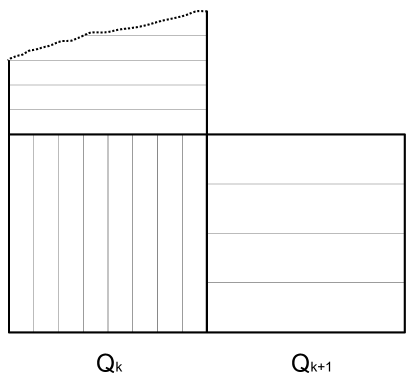
Figure 2. Construction of the rectangles in the $Q_{k}$’s

In the center of each of these subrectangles we label points $\{a_{0,j}^{1},\ldots,a_{0,j}^{{n_{j}}}\}$, so the distance between neighboring points is ${h\over n_{j}}$. Finally, we let

$$\omega_{0,j}^{n}={1\over n}\sum_{k=1}^{{n_{j}}}\delta_{a_{0,j}^{k}}$$

where the $a_{0,j}^{k}$ are defined above. In the worst-case scenario all vortices are located in a single cell with intervortex distance $O({h\over n})\approx n^{-{5\over 4}}$, and we will need to check that this conforms to the correct bound on $\rho_{a(0)}$.

We claim that $\omega_{0}^{n}\to\omega_{0}$ in $\mathcal{M}(\Omega)$. Let $f_{U}$ denote the average of $f$ on $U$. Then for $\chi\in C_{0}^{0}(\Omega)$, $\left|\int_{\Omega}\chi\left(\omega_{0}^{n}-\omega_{0}\right)\right|\leq\sum_{Q_{j}}\left|\int_{Q_{j}}(\chi-\chi_{Q_{j}})(\omega^{n}_{0}-\omega_{0})\right|+\sum_{Q_{j}}\left|\chi_{Q_{j}}\right|\left|\int_{Q_{j}}\omega_{0}^{n}-\omega_{0}\right|\to 0$ as $n\to\infty$ from (7.7), (7.8), and the continuity of $\chi$. Therefore, $\omega_{n}^{0}\to\omega_{0}$ in $\mathcal{M}(\Omega)$.

2. Finally, we claim that

(7.9) $$-{1\over n^{2}}\sum_{a_{0,i}^{j}\neq a_{0,k}^{\ell}}N_{n}(a_{0,i}^{j},a_{0,k}^{\ell})\lesssim 1.$$

Since the support of $\omega_{0}$ lies in a compact set away from the boundary, then

$$\min\{\operatorname{dist}(a_{0,j}^{k},\partial\Omega)\}\geq C>0$$

uniformly in $n$. Hence, we have $|H_{n}(a_{0,j}^{k},a_{0,i}^{\ell})|\leq C$ uniformly in $n$. In particular, to establish (7.9) it is sufficient to prove

$$-{1\over n^{2}}\sum_{a_{0,i}^{j}\neq a_{0,k}^{\ell}}\log|a_{0,i}^{j}-a_{0,k}^{\ell}|\lesssim 1.$$

We subdivide the sum into those vortex interactions arising from the same $Q_{j}$’s and those that arise from differing $Q_{k}$’s,

$$-{1\over n^{2}}\sum_{a_{0,i}^{j}\neq a_{0,k}^{\ell}}\log|a_{0,i}^{j}-a_{0,k}^{\ell}| =-{1\over n^{2}}\sum_{j}\sum_{k\neq\ell}\log|a_{0,j}^{k}-a_{0,j}^{\ell}|-{1\over n^{2}}\sum_{j\neq k}\sum_{i,\ell}\log|a_{0,j}^{i}-a_{0,k}^{\ell}|$$

$$=A+B$$

We now consider the sum $A$. Concentrating on a single $Q_{j}$, assume without loss of generality that the subrectangles are vertical and $a_{0,j}^{1}$ is located at the origin. Then the vortices in this square are located along the $x$-axis with $x$ values at $\{0,\Delta,2\Delta,\ldots,(n_{j}-1)\Delta\}$, where $\Delta={h\over n_{j}}$. Summing over the log interactions yields

$$-\sum_{k\neq\ell}\log|a_{0,j}^{k}-a_{0,j}^{\ell}| =-\left[(n_{j}-1)\log|\Delta|+(n_{j}-2)\log|2\Delta|+\cdots+\log|(n_{j}-1)\Delta|\right]$$

$$\leq{n_{j}(n_{j}-1)\over 2}\log\Delta^{-1}\leq{n^{2}_{j}\over 2}\log h^{-1}+{n_{j}^{2}\over 2}\log n$$

$$\leq 3n_{j}^{2}\log h^{-1},$$

since $\log h^{-1}={1\over 4}\log n$. Now summing over the $j$’s yields and using that ${n_{j}\over n}\leq{1\over 2\pi}\int_{Q_{j}}\omega_{0}$, we get

$$A =-{1\over n^{2}}\sum_{j}\sum_{k\neq\ell}\log|a_{0,j}^{k}-a_{0,j}^{\ell}|\lesssim{1\over n^{2}}\sum_{j}n_{j}^{2}\log h^{-1}$$

$$\lesssim\sum_{j}\log h^{-1}\int_{Q_{j}}\omega_{0}(y)\int_{Q_{j}}\omega_{0}(z)$$

$$\lesssim-\sum_{j}\int_{Q_{j}}\int_{Q_{j}}\omega_{0}(y)\log|y-z|\omega_{0}(z)dydz$$

Next we bound $B$. Let $p_{j}$ denote the center of the square $Q_{j}$. Due to the alternating alignment of the subrectangles in Figure 2, we see that $\left|\log|a_{0,j}^{i}-a_{0,k}^{\ell}|-\log|p_{j}-p_{k}|\right|\leq C$, even for neighboring squares. Therefore,

$$B =-{1\over n^{2}}\sum_{j\neq k}\sum_{i,\ell}\log|a_{0,j}^{i}-a_{0,k}^{\ell}|$$

$$=-{1\over n^{2}}\sum_{j\neq k}\sum_{i=1}^{n_{j}}\sum_{\ell=1}^{n_{k}}\log|a_{0,j}^{i}-a_{0,k}^{\ell}|$$

$$\leq C-{C\over n^{2}}\sum_{j\neq k}\sum_{i=1}^{n_{j}}\sum_{\ell=1}^{n_{k}}\log|p_{i}-p_{k}|=C-{C\over n^{2}}\sum_{j\neq k}{n_{j}}{n_{k}}\log|p_{i}-p_{k}|$$

$$\lesssim 1-\sum_{j\neq k}\log|p_{i}-p_{k}|\int_{Q_{j}}\omega_{0}(y)\int_{Q_{k}}\omega_{0}(z)$$

$$\lesssim 1-\sum_{j\neq k}\int_{Q_{j}}\int_{Q_{k}}\omega_{0}(y)\log|y-z|\omega_{0}(z)dydz$$

Combining $A$ and $B$ together we find

$$A+B \lesssim 1-\int_{\Omega}\int_{\Omega}\omega_{0}(y)\log|y-z|\omega_{0}(z)dydz$$

$$\lesssim 1+\left\|\omega_{0}\right\|_{\dot{H}^{-1}(\Omega)}\left\|\mu_{\operatorname{supp}(\omega_{0})}(y)\int\log|y-z|\omega_{0}(z)\right\|_{H^{1}(\Omega)}$$

$$\lesssim 1+\left\|\omega_{0}\right\|^{2}_{\dot{H}^{-1}}\lesssim 1,$$

where $\mu_{Q}$ is the characteristic function on $Q$.

3. Now we complete the proof of the hydrodynamic limit. Set $\varepsilon_{n}$ such that $n=|\log|\log|\log\varepsilon_{n}|||^{1\over 4}$ and

$$\tilde{\omega}_{n}(t)={1\over n}{e_{\varepsilon_{n}}(u_{\varepsilon_{n}}(t))\over\pi|\log\varepsilon_{n}|}.$$

Given the initial measure $\omega_{0}$, we build our initial data $u_{\varepsilon_{n}}(0)$ with vortices at $\{a_{0,j}^{k}\}$ as generated above, and satisfying the hypotheses of Theorem 1.1. Such data can be constructed following Lemma 14 of [23]. Then since the energy is decreasing in time and using (6.13), we obtain for a subsequence that $\tilde{\omega}_{n}\to\tilde{\omega}$ in $\mathcal{M}(\Omega\times[0,\infty))$. Furthermore, the intervortex distance is no worse than

$$\rho_{a(0)}\geq C{h\over n}\geq Cn^{-{3\over 2}}\geq C\left|\log\left|\log\left|\log\varepsilon_{n}\right|\right|\right|^{-{3\over 8}}\geq\left|\log\left|\log\left|\log\varepsilon_{n}\right|\right|\right|^{-{1\over 3}};$$

therefore, both $n$ and $\rho_{a(0)}$ satisfy the requirements of Proposition 3.3.

From Proposition 7.1 we obtain that $\omega_{n}=\frac{1}{n}\sum\delta_{a_{j}(t)}$ converges to some $\omega$ that is an interior weak solution of (1.21). By Theorem 1.1, we see that $\omega_{n}-\tilde{\omega}_{n}\to 0$ in distribution, and so $\tilde{\omega}=\omega$ also solves (1.21).

∎

Proof of Theorem 1.4.

The proof of Theorem 1.4 follows along the same lines as the proof of Theorem 1.3. In particular we use assumptions (1.23)-(1.26) in order to satisfy the hypotheses of Theorem 1.1. Next, assumptions (1.25)-(1.26) ensure the long-time existence of the vortex dynamics via Proposition 3.3. Finally, assumption (1.27) allows us to use the ODE to PDE result, Proposition 7.1. The proof follows.

∎

References

- [1] Ambrosio, L., Serfaty, S. A gradient flow approach to an evolution problem arising in superconductivity. Comm. Pure Appl. Math. 61, 11 (2008), 1495–1539.
- [2] Ambrosio, L., Mainini, E., Serfaty, S. Gradient flow of the Chapman-Rubinstein-Schatzman model for signed vortices. Ann. IHP, Analyse nonlinéaire. 28, 2 (2011), 217–246.
- [3] Bethuel, F., Brezis, H., Hélein, F.: Ginzburg-Landau Vortices. Progress in Nonlinear Differential Equations and their Applications, 13. Birkhäuser, Boston, 1994
- [4] Bethuel, F., Orlandi, G., Smets, D.: Collisions and phase-vortex interactions in dissipative Ginzburg-Landau dynamics. Duke Math. J. 130, 523–614 (2005)
- [5] Brezis, H., Coron, J.-M., Lieb, E.: Harmonic maps with defects. Comm. Math. Phys. 107, 649-705 (1986)
- [6] Chapman, S. J. A Hierarchy of Models for Type-II Superconductors SIAM Review 42 (2000), 555–598.
- [7] Chapman, S. J., Rubinstein, J., Schatzman, M. A mean-field model of superconducting vortices. European J. Appl. Math. 7 (1996), 97–111.
- [8] Colliander, J.E., Jerrard, R.L.: Ginzburg-Landau vortices: weak stability and Schrödinger equation dynamics. J. Anal. Math. 77, 129–205 (1999)
- [9] Delort, J.-M., Existence de nappes de tourbillon en dimension deux, J. Amer. Math. Soc., 4 (1991), 553–586.
- [10] DiPerna, R. J.,; Majda, A. J., Concentrations in regularizations for 2-D incompressible flow, Comm. Pure Appl. Math. 40, (1987), 301–345.
- [11] Dorsey, A. T. Vortex motion and the Hall effect in type-II superconductors: A time-dependent Ginzburg-Landau theory approach. Phys. Rev. B 46, 13 (Oct 1992), 8376–8392.
- [12] E, W.: Dynamics of vortices in Ginzburg-Landau theories with applications to superconductivity. Phys. D 77, 383–404 (1994)
- [13] E, W. Dynamics of vortex liquids in Ginzburg-Landau theories with applications to superconductivity, Phys. Rev. B 50, (1994), 1126–1135.
- [14] Essmann, U.; Träuble, H. The flux-line arrangement in the ”intermediate state” of type II superconductors” Physics Letters 27A (1968), 156–157.
- [15] Evans, L. C. Partial differential equations. Graduate Studies in Mathematics, 19. American Mathematical Society, Providence, RI, 1998.
- [16] Evans, L. C.; Müller, S. Hardy spaces and the two-dimensional Euler equations with nonnegative vorticity. J. Amer. Math. Soc. 7 (1994), no. 1, 199–219.
- [17] Lopes Filho, M. C., Nussenzveig Lopes, H. J., Xin, Z. Existence of vortex sheets with reflection symmetry in two space dimensions. Arch. Ration. Mech. Anal. 158 (2001), no. 3, 235–257.
- [18] Jerrard, R.L.: Vortex dynamics for the Ginzburg–Landau wave equation. Calc. Var. Partial Differential Equations 9, 683–688 (1999)
- [19] Jerrard, R. L. Lower bounds for generalized Ginzburg-Landau functionals, SIAM J. Math. Anal. 30 (1999), 721–746.
- [20] Jerrard, R.L., Soner, H.M.: The Jacobian and the Ginzburg-Landau energy. Calc. Var. Partial Differential Equations 14, 151–191 (2002)
- [21] Jerrard, R.L., Soner, H.M.: Dynamics of Ginzburg–Landau vortices. Arch. Rational Mech. Anal. 142, 99–125 (1998)
- [22] Jerrard, R.L., Spirn, D.: Refined Jacobian estimates for Ginzburg-Landau functionals. Indiana Univ. Math. Jour. 56, 135–186 (2007)
- [23] Jerrard, R.L., Spirn, D.: Refined Jacobian estimates and Gross-Pitaevsky vortex dynamics Arch. Ration. Mech. Anal. (2008)
- [24] Kopnin, N. B., Ivlev, B. I., and Kalatsky, V. A. The flux-flow hall effect in type ii superconductors. an explanation of the sign reversal. Journal of Low Temperature Physics 90, 1 (01 1993), 1–13.
- [25] Kurzke, M., Melcher, C., Moser, R.: Vortex motion for the Landau-Lifshitz-Gilbert equation with spin transfer torque. SIAM J. Math. Anal. 43, 1099–1121.
- [26] Kurzke, M., Melcher, C., Moser, R., and Spirn, D. Dynamics for Ginzburg-Landau vortices under a mixed flow. Indiana Univ. Math. J. 58, 6 (2009), 2597–2621.
- [27] Kurzke, M., Spirn, D. -stability and vortex motion in type II superconductors. Communications in Partial Differential Equations 36, 2 (2011), 256 – 292.
- [28] Kurzke, M., Spirn, D.: Quantitative equipartition of the Ginzburg-Landau energy with applications. Indiana U. J. Math. 59, 6 (2010), 2077–2092.
- [29] Lin, F.-H.: Some dynamical properties of Ginzburg-Landau vortices. Comm. Pure Appl. Math. 49, 323–359 (1996)
- [30] Lin, F.-H.: Vortex dynamics for the nonlinear wave equation. Comm. Pure Appl. Math.52, 737–761 (1999)
- [31] Lin, F.H.; Lin, T.C. Minimax solutions of the Ginzburg-Landau equations. Selecta Math. 3 (1997), 99–113.
- [32] Lin, F. H.; Zhang, P. On the hydrodynamic limit of Ginzburg-Landau vortices. Discrete Contin. Dynamic Systems 6 (2000), no. 1, 121–142.
- [33] Lin, F.; Zhang, P. On the hydrodynamic limit of Ginzburg-Landau wave vortices. Comm. Pure Appl. Math. 55, 7 (2002), 831–856.
- [34] Liu, J.G.; Xin, Z. Convergence of the point vortex method for 2-D vortex sheet. Math. Comp. 70 (2001), 595–606.
- [35] Liu, J.G.; Xin, Z. Convergence of Vortex Methods for Weak Solutions to the 2-D Euler Equations with Vortex Sheet Data. Comm. Pure Appl. Math. 48 (1995), 611–628.
- [36] Majda, A.J. Remarks on weak solutions for vortex sheets with a distinguished sign. Indiana Univ. Math. J. 42 (1993), 921–939.
- [37] Miot, E. Dynamics of vortices for the complex Ginzburg-Landau equation. Anal. PDE 2, 2 (2009), 159–186.
- [38] Peres, L.; Rubinstein, J., Vortex dynamics in Ginzburg-Landau models, Phys. D, 64 (1993), 299–309.
- [39] Roitberg, Y.: Elliptic Boundary Value Problems in the Space of Distributions. Mathematics and its Applications, 498. Kluwer Academic Publications, Dordrecht, 1999
- [40] Sandier, E. Lower bounds for the energy of unit vector fields and applications. J. Funct. Anal. 152 (1998), 379–403.
- [41] Sandier, E., Serfaty, S.: Gamma-convergence of gradient flows with applications to Ginzburg-Landau. Comm. Pure Appl. Math. 57, 1627–1672 (2004)
- [42] Sandier, E., Serfaty, S. Product Estimates for Ginzburg-Landau and corollaries. J. Funct. Anal. 211 (2004), no. 1, 219–244.
- [43] Sandier, E., Soret, M. -Valued Harmonic Maps with High Topological Degree: Asymptotic Behavior of the Singular Set. Potential Anal. 13 (2000), 169–184.
- [44] Schochet, S., The point vortex method for periodic weak solutions of the 2D Euler equations, Comm. Pure Appl. Math., 49 (1996) 911–965.
- [45] Serfaty, S. Vortex collisions and energy-dissipation rates in the Ginzburg-Landau heat flow, part I: Study of the perturbed Ginzburg-Landau equation, Journal Eur. Math Society , 9, No 2, (2007), 177–217.
- [46] Serfaty, S. Vortex collisions and energy-dissipation rates in the Ginzburg-Landau heat flow. II. The dynamics. J. Eur. Math. Soc. (JEMS) 9 (2007), no. 3, 383–426.
- [47] Serfaty, S. Gamma-convergence of gradient flows on Hilbert and metric spaces and applications, Discrete Contin. Dyn. Syst. Ser. A 31, 4 (2011), 1427–1451.
- [48] Serfaty, S., Tice, I. Ginzburg-Landau vortex dynamics with pinning and strong applied currents. Arch. Rat. Mech. Anal. 201 (2011), 413–464.
- [49] Spirn, D. Vortex dynamics of the full time-dependent Ginzburg-Landau model. Comm. Pure Appl. Math. 55 (2002), 537–581.