Fault-tolerant Algorithms for Tick-Generation in Asynchronous Logic:
Robust Pulse Generation Fault-tolerant Algorithms for Tick-Generation in Asynchronous Logic: Robust Pulse Generation

Abstract

Today’s hardware technology presents a new challenge in designing robust systems. Deep submicron VLSI technology introduced transient and permanent faults that were never considered in low-level system designs in the past. Still, robustness of that part of the system is crucial and needs to be guaranteed for any successful product. Distributed systems, on the other hand, have been dealing with similar issues for decades. However, neither the basic abstractions nor the complexity of contemporary fault-tolerant distributed algorithms match the peculiarities of hardware implementations.

This paper is intended to be part of an attempt striving to overcome this gap between theory and practice for the clock synchronization problem. Solving this task sufficiently well will allow to build a very robust high-precision clocking system for hardware designs like systems-on-chips in critical applications. As our first building block, we describe and prove correct a novel Byzantine fault-tolerant self-stabilizing pulse synchronization protocol, which can be implemented using standard asynchronous digital logic. Despite the strict limitations introduced by hardware designs, it offers optimal resilience and smaller complexity than all existing protocols.

1 Introduction & Related Work

With today’s deep submicron technology running at GHz clock speeds [20], disseminating the high-speed clock throughout a very large scale integrated (VLSI) circuit, with negligible skew, is difficult and costly [2, 3, 12, 24, 29]. Systems-on-chip are hence increasingly designed globally asynchronous locally synchronous (GALS) [4], where different parts of the chip use different local clock signals. Two main types of clocking schemes for GALS systems exist, namely, (i) those where the local clock signals are unrelated, and (ii) multi-synchronous ones that provide a certain degree of synchrony between local clock signals [30, 34].

GALS systems clocked by type (i) permanently bear the risk of metastable upsets when conveying information from one clock domain to another. To explain the issue, consider a physical implementation of a bistable storage element, like a register cell, which can be accessed by read and write operations concurrently. It can be shown that two operations (like two writes with different values) occurring very closely to each other can cause the storage cell to attain neither of its two stable states for an unbounded time [23], and thereby, during an unbounded time afterwards, successive reads may return none of the stable states. Although the probability of a single upset is very small, one has to take into account that every bit of transmitted information across clock domains is a candidate for an upset. Elaborate synchronizers [8, 21, 28] are the only means for achieving an acceptably low probability for metastable upsets here.

This problem can be circumvented in clocking schemes of type (ii): Common synchrony properties offered by multi-synchronous clocking systems are:

• bounded skew, i.e., bounded maximum time between the occurence of any two matching clock transitions of any two local clock signals. Thereby, in classic clock synchronization, two clock transitions are matching iff they are both the $k^{\text{th}}$, $k\geq 1$, clock transition of a local clock.

• bounded accuracy, i.e., bounded minimum and maximum time between the occurence of any two successive clock transitions of any local clock signal.

Type (ii) clocking schemes are particularly beneficial from a designer’s point of view, since they combine the convenient local synchrony of a GALS system with a global time base across the whole chip. It has been shown in [27] that these properties indeed facilitate metastability-free high-speed communication across clock domains.

The decreasing structure sizes of deep submicron technology also resulted in an increased likelihood of chip components failing during operation: Reduced voltage swing and smaller critical charges make circuits more susceptible to ionized particle hits, crosstalk, and electromagnetic interference [5, 18]. Fault-tolerance hence becomes an increasingly pressing issue in chip design. Unfortunately, faulty components may behave non-benign in many ways. They may perform signal transitions at arbitrary times and even convey inconsistent information to their successor components if their outgoing communication channels are affected by a failure. This forces to model faulty components as unrestricted, i.e., Byzantine, if a high fault coverage is to be guaranteed.

The darts fault-tolerant clock generation approach [15, 17] developed by some of the authors of this paper is a Byzantine fault-tolerant multi-synchronous clocking scheme. darts comprises a set of modules, each of which generates a local clock signal for a single clock domain. The darts modules (nodes) are synchronized to each other to within a few clock cycles. This is achieved by exchanging binary clock signals only, via single wires. The basic idea behind darts is to employ a simple fault-tolerant distributed algorithm [35]—based on Srikanth & Toueg’s consistent broadcasting primitive [31]—implemented in asynchronous digital logic. An important property of the darts clocking scheme is that it guarantees that no metastable upsets occur during fault-free executions. For executions with faults, metastable upsets cannot be ruled out: Since Byzantine faulty components are allowed to issue unrelated read and write accesses by definition, the same arguments as for clocking schemes of type (i) apply. However, in [13], it was shown that by proper chip design the probability of a Byzantine component leading to a metastable upset of darts can be made arbitrarily small.

Although both theoretical analysis and experimental evaluation revealed many attractive additional features of darts, like guaranteed startup, automatic adaption to current operating conditions, etc., there is room for improvement. The most obvious drawback of darts is its inability to support late joining and restarting of nodes, and, more generally, its lack of self-stabilization properties. If, for some reasons, more than a third of the darts nodes ever become faulty, the system cannot be guaranteed to resume normal operation even if all failures cease. Even worse, simple transient faults such as radiation- or crosstalk-induced additional (or omitted) clock ticks accumulate over time to arbitrarily large skews in an otherwise benign execution.

Byzantine-tolerant self-stabilization, on the other hand, is the major strength of a number of protocols [1, 6, 9, 19, 22] primarily devised for distributed systems. Of particular interest in the above context is the work on self-stabilizing pulse synchronization, where the purpose is to generate well-separated anonymous pulses that are synchronized at all correct nodes. This facilitates self-stabilizing clock synchronization, as agreement on a time window permits to simulate a synchronous protocol in a bounded-delay system. Beyond optimal (i.e., $\lceil n/3\rceil-1$, c.f. [26]) resilience, an attractive feature of these protocols is a small stabilization time [1, 6, 19, 22], which is crucial for applications with stringent availability requirements. In particular, [1] synchronizes clocks in expected constant time in a synchronous system. Given any pulse synchronization protocol stabilizing in a bounded-delay system in expected time $T$, this implies an expected $(T+\mathcal{O}(1))$-stabilizing clock synchronization protocol.

Nonetheless, it remains open whether a (with respect to the number of nodes $n$) sublinear convergence time can be achieved: While the classical consensus lower bound of $f+1$ rounds for synchronous, deterministic algorithms in a system with $f<n/3$ faults [11] proves that exact agreement on a clock value requires at least $f+1\in\Omega(n)$ deterministic rounds, one has to face the fact that only approximate agreement on the current time is achievable in a bounded-delay system anyway. However, no non-trivial lower bounds on approximate deterministic synchronization or the exact problem with randomization are known by now.

Note that existing synchronization algorithms, in particular those that do not rely on pulse synchronization, have deficiencies rendering them unsuitable in our context. For example, they have exponential convergence time [9], require the relative drift of the nodes’ local clocks to be very small [7, 22], provide larger skew only [22] or make use of linear-sized messages [6]. Furthermore, standard models used by the distributed systems community do not account for metastability, resulting in the same to be true for the existing solutions.

It is hence natural to explore ways of combining and extending the above lines of research. The present paper is the first step towards this goal.

Detailed contributions. We describe and prove correct the novel FATAL pulse synchronization protocol, which facilitates a direct implementation in standard asynchronous digital logic. It self-stabilizes within $\mathcal{O}(n)$ time with probability $1-2^{n-f}$, in the presence of up to $\lceil n/3\rceil-1$ Byzantine faulty nodes, and is metastability-free by construction after stabilization in failure-free runs. While executing the protocol, non-faulty nodes broadcast a constant number of bits in constant time. In terms of distributed message complexity, this implies that stabilization is achieved after broadcasting $\mathcal{O}(n)$ messages of size $\mathcal{O}(1)$, improving by factor $\Omega(n)$ on the number of bits transmitted by previous algorithms. The protocol can sustain large relative clock drifts of more than $10\%$, which is crucial if the local clock sources are simple ring oscillators (uncompensated ring oscillators suffer from clock drifts of up to $9\%$ [32]). If the number of faults is not overwhelming, i.e., a majority of at least $n-f$ nodes continues to execute the protocol in an orderly fashion, recovering nodes and late joiners (re)synchronize in constant time. This property is highly desirable in practical systems, in particular in combination with Byzantine fault-tolerance: Even if nodes randomly experience transient faults on a regular basis, quick recovery ensures that the mean time until failure of the system as a whole is substantially increased. All this is achieved against a powerful adversary that, at time $t$, knows the whole history of the system up to time $t+\varepsilon$ (where $\varepsilon>0$ is infinitesimally small) and does not need to choose the set of faulty nodes in advance. Apart from bounded drifts and communication delays, our solution solely requires that receivers can unambiguously identify the sender of a message, which is a property that arises naturally in hardware designs.

We also describe how the pulse synchronization protocol can be implemented using asynchronous digital logic. Moreover, we sketch how the pulse synchronization protocol will be integrated with darts clocks to build a high-precision self-stabilizing clocking system for multi-synchronous GALS. The basic idea of our integration is to let the pulse synchronization protocol non-intrusively monitor the operation of darts clocks and to recover darts clocks that run abnormally. Like the original darts, the joint system is metastability-free in failure-free runs after stabilization. During stabilization, the fact that nodes merely undergo a constant number of state transitions in constant time ensures a very small probability of metastable upsets.

2 Model

Our formal framework will be tied to the peculiarities of hardware designs, which consist of modules that continuously compute their output signals based on their input signals. Following [14, 16], we define (the trace of) a signal to be a timed event trace over a finite alphabet $\mathbb{S}$ of possible signal states: Formally, signal $\sigma\subseteq\mathbb{S}\times\mathbb{R}_{0}^{+}$. All times and time intervals refer to a global reference time taken from $\mathbb{R}_{0}^{+}$, that is, signals describe the system’s behaviour from time 0 on. The elements of $\sigma$ are called events, and for each event $(s,t)$ we call $s$ the state of event $(s,t)$ and $t$ the time of event $(s,t)$. In general, a signal $\sigma$ is required to fulfill the following conditions: (i) for each time interval $[t^{-},t^{+}]\subseteq\mathbb{R}_{0}^{+}$ of finite length, the number of events in $\sigma$ with times within $[t^{-},t^{+}]$ is finite, (ii) from $(s,t)\in\sigma$ and $(s^{\prime},t)\in\sigma$ follows that $s=s^{\prime}$, and (iii) there exists an event at time $0$ in $\sigma$.

Note that our definition allows for events $(s,t)$ and $(s,t^{\prime})\in\sigma$, where $t<t^{\prime}$, without having an event $(s^{\prime},t^{\prime\prime})\in\sigma$ with $s^{\prime}\neq s$ and $t<t^{\prime\prime}<t^{\prime}$. In this case, we call event $(s,t^{\prime})$ idempotent. Two signals $\sigma$ and $\sigma^{\prime}$ are equivalent, iff they differ in idempotent events only. We identify all signals of an equivalence class, as they describe the same physical signal. Each equivalence class $[\sigma]$ of signals contains a unique signal $\sigma_{0}$ having no idempotent events. We say that signal $\sigma$ switches to $s$ at time $t$ iff event $(s,t)\in\sigma_{0}$.

The state of signal $\sigma$ at time $t\in\mathbb{R}_{0}^{+}$, denoted by $\sigma(t)$, is given by the state of the event with the maximum time not greater than $t$. Because of (i), (ii) and (iii), $\sigma(t)$ is well defined for each time $t\in\mathbb{R}_{0}^{+}$. Note that $\sigma$’s state function in fact depends on $[\sigma]$ only, i.e., we may add or remove idempotent events at will without changing the state function.

Distributed System

On the topmost level of abstraction, we see the system as a set of $V=\{1,\ldots,n\}$ physically remote nodes that communicate by means of channels. In the context of a VLSI circuit, “physically remote” actually refers to quite small distances (centimeters or even less). However, at gigahertz frequencies, a local state transition will not be observed remotely within a time that is negligible compared to clock speeds. We stress this point, since it is crucial that different clocks (and their attached logic) are not too close to each other, as otherwise they might fail due to the same event such as a particle hit. This would render it pointless to devise a system that is resilient to a certain fraction of the nodes failing.

Each node $i$ comprises a number of input ports, namely $S_{i,j}$ for each node $j$, an output port $S_{i}$, and a set of local ports, introduced later on. An execution of the distributed system assigns to each port of each node a signal. For convenience of notation, for any port $p$, we refer to the signal assigned to port $p$ simply by signal $p$. We say that node $i$ is in state $s$ at time $t$ iff $S_{i}(t)=s$. We further say that node $i$ switches to state $s$ at time $t$ iff signal $S_{i}$ switches to $s$ at time $t$.

Nodes exchange their states via the channels between them: for each pair of nodes $i,j$, output port $S_{i}$ is connected to input port $S_{j,i}$ by a FIFO channel from $i$ to $j$. Note that this includes a channel from $i$ to $i$ itself. Intuitively, $S_{i}$ being connected to $S_{j,i}$ by a (non-faulty) channel means that $S_{j,i}(\cdot)$ should mimic $S_{i}(\cdot)$, however, with a slight delay accounting for the time it takes the signal to propagate. In contrast to an asynchronous system, this delay is bounded by the maximum delay $d>0$.

Formally we define: The channel from node $i$ to $j$ is said to be correct during $[t^{-},t^{+}]$ iff there exists a function $\tau_{i,j}:\mathbb{R}_{0}^{+}\to\mathbb{R}_{0}^{+}$, called the channel’s delay function, such that: (i) $\tau_{i,j}$ is continuous and strictly increasing, (ii) $\forall t\in[t^{-},t^{+}]:0\leq\tau_{i,j}(t)-t<d$, and (iii) for each $t\in[t^{-},t^{+}]$, $(s,\tau_{i,j}(t))\in S_{j,i}\Leftrightarrow(s,t)\in S_{i}$. We say that node $i$ observes node $j$ in state $s$ at time $t$ if $S_{i,j}(t)=s$.

Clocks and Timeouts

Nodes are never aware of the current reference time and we also do not require the reference time to resemble Newtonian “real” time. Rather we allow for physical clocks that run arbitrarily fast or slow, as long as their speeds are close to each other in comparison. One may hence think of the reference time as progressing at the speed of the currently slowest correct clock. In this framework, nodes essentially make use of bounded clocks with bounded drift.

Formally, clock rates are within $[1,\vartheta]$ (with respect to reference time), where $\vartheta>1$ is constant and $\vartheta-1$ is the (maximum) clock drift. A clock $C$ is a continuous, strictly increasing function $C:\mathbb{R}^{+}_{0}\to\mathbb{R}^{+}_{0}$ mapping reference time to some local time. Clock $C$ is said to be correct during $[t^{-},t^{+}]\subseteq\mathbb{R}^{+}_{0}$ iff we have for any $t,t^{\prime}\in[t^{-},t^{+}]$, $t<t^{\prime}$, that $t^{\prime}-t\leq C(t^{\prime})-C(t)\leq\vartheta(t^{\prime}-t)$. Each node comprises a set of clocks assigned to it, which allow the node to estimate the progress of reference time.

Instead of directly accessing the value of their clocks, nodes have access to so-called timeout ports of watchdog timers. A timeout is a triple $(T,s,C)$, where $T\in\mathbb{R}^{+}$ is a duration, $s\in\mathbb{S}$ is a state, and $C$ is a clock, say of node $i$. Each timeout $(T,s,C)$ has a corresponding timeout port $\operatorname{Time}_{T,s,C}$, being part of node $i$’s local ports. Signal $\operatorname{Time}_{T,s,C}$ is Boolean, that is, its possible states are from the set $\{0,1\}$. We say that timeout $(T,s,C)$ is correct during $[t^{-},t^{+}]\subseteq\mathbb{R}^{+}_{0}$ iff clock $C$ is correct during $[t^{-},t^{+}]$ and the following holds:

1. For each time $t_{s}\in[t^{-},t^{+}]$ when node $i$ switches to state $s$, there is a time $t\in[t_{s},\tau_{i,i}(t_{s})]$ such that $(T,s,C)$ is reset, i.e., $(0,t)\in\operatorname{Time}_{T,s,C}$. This is a one-to-one correspondence, i.e., $(T,s,C)$ is not reset at any other times.

2. For a time $t\in[t^{-},t^{+}]$, denote by $t_{0}$ the supremum of all times from $[t^{-},t]$ when $(T,s,C)$ is reset. Then it holds that $(1,t)\in\operatorname{Time}_{T,s,C}$ iff $C(t)-C(t_{0})=T$. Again, this is a one-to-one correspondence.

We say that timeout $(T,s,C)$ expires at time $t$ iff $\operatorname{Time}_{T,s,C}$ switches to $1$ at time $t$, and it is expired at time $t$ iff $\operatorname{Time}_{T,s,C}(t)=1$. For notational convenience, we will omit the clock $C$ and simply write $(T,s)$ for both the timeout and its signal.

A randomized timeout is a triple $({\cal D},s,C)$, where ${\cal D}$ is a bounded random distribution on $\mathbb{R}^{+}_{0}$, $s\in\mathbb{S}$ is a state, and $C$ is a clock. Its corresponding timeout port $\operatorname{Time}_{{\cal D},s,C}$ behaves very similar to the one of an ordinary timeout, except that whenever it is reset, the local time that passes until it expires next—provided that it is not reset again before that happens—follows the distribution $\cal D$. Formally, $({\cal D},s,C)$ is correct during $[t^{-},t^{+}]\subseteq\mathbb{R}^{+}_{0}$, if $C$ is correct during $[t^{-},t^{+}]$ and the following holds:

1. For each time $t_{s}\in[t^{-},t^{+}]$ when node $i$ switches to state $s$, there is a time $t\in[t_{s},\tau_{i,i}(t_{s})]$ such that $({\cal D},s,C)$ is reset, i.e., $(0,t)\in\operatorname{Time}_{{\cal D},s,C}$. This is a one-to-one correspondence, i.e., $({\cal D},s,C)$ is not reset at any other times.

2. For a time $t\in[t^{-},t^{+}]$, denote by $t_{0}$ the supremum of all times from $[t^{-},t]$ when $({\cal D},s,C)$ is reset. Let $\mu:\mathbb{R}_{0}^{+}\to\mathbb{R}_{0}^{+}$ denote the density of $\cal D$. Then $(1,t)\in\operatorname{Time}_{{\cal D},s,C}$ “with probability $\mu(C(t)-C(t_{0}))$” and we require that the probability of $(1,t)\in\operatorname{Time}_{{\cal D},s,C}$—conditional to $t_{0}$ and $C$ on $[t_{0},t]$ being given—is independent of the system’s state at times smaller than $t$. More precisely, if superscript $\cal E$ identifies variables in execution $\cal E$ and $t_{0}^{\prime}$ is the infimum of all times from $(t_{0},t^{+}]$ when node $i$ switches to state $s$, then we demand for any $[\tau^{-},\tau^{+}]\subseteq[t_{0},t_{0}^{\prime}]$ that

   $$P\left[\exists t^{\prime}\in[\tau^{-},\tau^{+}]:(1,t^{\prime})\in\operatorname{Time}_{{\cal D},s,C}\,\Big{|}\,t_{0}^{\cal E}=t_{0}\wedge C\big{|}_{[t_{0},t^{\prime}]}^{\cal E}=C\big{|}_{[t_{0},t^{\prime}]}\right]=\int_{\tau^{-}}^{\tau^{+}}\mu(C(\tau)-C(t_{0}))~{}d\tau,$$

   independently of ${\cal E}\big{|}_{[0,\tau^{-})}$.

We will apply the same notational conventions to randomized timeouts as we do for regular timeouts.

Note that, strictly speaking, this definition does not induce a random variable describing the time $t^{\prime}\in[t_{0},t_{0}^{\prime})$ satisfying that $(1,t^{\prime})\in\operatorname{Time}_{{\cal D},s,C}$. However, for the state of the timeout port, we get the meaningful statement that for any $t^{\prime}\in[t_{0},t_{0}^{\prime})$,

$$P[\operatorname{Time}_{{\cal D},s,C}\mbox{ switches to $1$ during }[t_{0},t^{\prime}]]=\int_{t_{0}}^{t^{\prime}}\mu(C(t^{\prime})-C(t_{0}))~{}d\tau.$$

The reason for phrasing the definition in the above more cumbersome way is that we want to guarantee that an adversary knowing the full present state of the system and memorizing its whole history cannot reliably predict when the timeout will expire.

We remark that these definitions allow for different timeouts to be driven by the same clock, implying that an adversary may derive some information on the state of a randomized timeout before it expires from the node’s behaviour, even if it cannot directly access the values of the clock driving the timeout. This is crucial for implementability, as it might be very difficult to guarantee that the behaviour of a dedicated clock that drives a randomized timeout is indeed independent of the execution of the algorithm.

Memory Flags

Besides timeout and randomized timeout ports, another kind of node $i$’s local ports are memory flags. For each state $s\in\mathbb{S}$ and each node $j\in V$, $\operatorname{Mem}_{i,j,s}$ is a local port of node $i$. It is used to memorize whether node $i$ has observed node $j$ in state $s$ since the last reset of the flag. We say that node $i$ memorizes node $j$ in state $s$ at time $t$ if $\operatorname{Mem}_{i,j,s}(t)=1$. Formally, we require that signal $\operatorname{Mem}_{i,j,s}$ switches to $1$ at time $t$ iff node $i$ observes node $j$ in state $s$ at time $t$ and $\operatorname{Mem}_{i,j,s}$ is not already in state $1$. The times $t$ when $\operatorname{Mem}_{i,j,s}$ is reset, i.e., $(0,t)\in\operatorname{Mem}_{i,j,s}$, are specified by node $i$’s state machine, which is introduced next.

State Machine

It remains to specify how nodes switch states and when they reset memory flags. We do this by means of state machines that may attain states from the finite alphabet $\mathbb{S}$. A node’s state machine is specified by (i) the set $\mathbb{S}$, (ii) a function $tr$, called the transition function, from ${\cal T}\subseteq\mathbb{S}^{2}$ to the set of Boolean predicates on the alphabet consisting of expressions “$p=s$” (used for expressing guards), where $p$ is from the node’s input and local ports and $s$ is from the set of possible states of signal $p$, and (iii) a function $re$, called the reset function, from $\cal T$ to the power set of the node’s memory flags.

Intuitively, the transition function specifies the conditions (guards) under which a node switches states, and the reset function determines which memory flags to reset upon the state change. Formally, let $P$ be a predicate on node $i$’s input and local ports. We define $P$ holds at time $t$ by structural induction: If $P$ is equal to $p=s$, where $p$ is one of node $i$’s input and local ports and $s$ is one of the states signal $p$ can obtain, then $P$ holds at time $t$ iff $p(t)=s$. Otherwise, if $P$ is of the form $\neg P_{1}$, $P_{1}\wedge P_{2}$, or $P_{1}\vee P_{2}$, we define $P$ holds at time $t$ in the straightforward manner.

We say node $i$ follows its state machine during $[t^{-},t^{+}]$ iff the following holds: Assume node $i$ observes itself in state $s\in\mathbb{S}$ at time $t\in[t^{-},t^{+}]$, i.e., $S_{i,i}(t)=s$. Then, for each $(s,s^{\prime})\in\cal T$, both:

1. Node $i$ switches to state $s^{\prime}$ at time $t$ iff $tr(s,s^{\prime})$ holds at time $t$ and $i$ is not already in state $s^{\prime}$.

2. Node $i$ resets memory flag $m$ at some time in the interval $[t,\tau_{i,i}(t)]$ iff $m\in re(s,s^{\prime})$ and $i$ switches from state $s$ to state $s^{\prime}$ at time $t$. This correspondence is one-to-one.

A node is defined to be non-faulty during $[t^{-},t^{+}]$ iff during $[t^{-},t^{+}]$ all its timeouts and randomized timeouts are correct and it follows its state machine. If it employs multiple state machines (see below), it needs to follow all of them.

In contrast, a faulty node may change states arbitrarily. Note that while a faulty node may be forced to send consistent output state signals to all other nodes if its channels remain correct, there is no way to guarantee that this still holds true if channels are faulty.

Metastability

In our discrete system model, the effect of metastability is captured by the lacking capability of state machines to instantaneously take on new states: Node $i$ decides on state transitions based on the delayed status of port $S_{i,i}$ instead of its “true” current state $S_{i}$. This non-zero delay from $S_{i}$ to $S_{i,i}$ bears the potential for metastability, as a successful state transition can only be guaranteed if after a transition guard from some state $s$ to some state $s^{\prime}$ becomes true, all other transition guards from $s$ to $s^{\prime\prime}\neq s^{\prime}$ remain false during this delay at least.

This is exemplified in the following scenario: Assume node $i$ is in state $s$ at some time $t$. However, since it switched to $s$ only very recently, it still observes itself in state $s^{\prime}\neq s$ at time $t$ via $S_{i,i}$. Given that there is a transition $(s^{\prime},s^{\prime\prime})$ in $\cal T$, $s^{\prime\prime}\neq s$, whose condition is fulfilled at time $t$, it will switch to state $s^{\prime\prime}$ at time $t$ (although state $s$ has not even stabilized yet). That is, due to the discrepancy between $S_{i,i}$ and $S_{i}$, node $i$ switches from state $s$ to state $s^{\prime\prime}$ at time $t$ even if $(s,s^{\prime\prime})$ is not in ${\cal T}$ at all. In a physical chip design, this premature change of state might even result in inconsistent operations on the local memory, up to the point where it cannot be properly described in terms of $\mathbb{S}$, and thus in terms of our discrete model, anymore. Even worse, the state of $i$ is part of the local memory and the node’s state signal may attain an undefined value that is propagated to other nodes and their memory. While avoiding the latter is the task of the input ports of a non-faulty node, our goal is to prevent this erroneous behaviour in situations where input ports attain legitimate values only.

Therefore, we define node $i$ to be metastability-free, if the situation described above does not occur.

Definition 2.1 (Metastability-Freedom).

Node $i\in V$ is called metastability-free during $[t^{-},t^{+}]$, iff for each time $t\in[t^{-},t^{+}]$ when $i$ switches to some state $s\in\mathbb{S}$, it holds that $\tau_{i,i}(t)<t^{\prime}$, where $t^{\prime}$ is the infimum of all times in $(t,t^{+}]$ when $i$ switches to some state $s^{\prime}\in\mathbb{S}$.

Multiple State Machines

In some situations the previous definitions are too stringent, as there might be different “components” of a node’s state machine that act concurrently and independently, mostly relying on signals from disjoint input ports or orthogonal components of a signal. We model this by permitting that nodes run several state machines in parallel. All these state machines share the input and local ports of the respective node and are required to have disjoint state spaces. If node $i$ runs state machines $M_{1},\ldots,M_{k}$, node $i$’s output signal is the product of the output signals of the individual machines. Formally we define: Each of the state machines $M_{j}$, $1\leq j\leq k$, has an additional own output port $s_{j}$. The state of node $i$’s output port $S_{i}$ at any time $t$ is given by $S_{i}(t):=(s_{1}(t),\ldots,s_{k}(t))$, where the signals of ports $s_{1},\ldots,s_{k}$ are definied analogously to the signals of the output ports of state machines in the single state machine case, each. Note that by this definition, the only (local) means for node $i$’s state machines to interact with each other is by reading the delayed state signal $S_{i,i}$.

We say that node $i$’s state machine $M_{j}$ is in state $s$ at time $t$ iff $s_{j}(t)=s$, where $S_{i}(t)=(s_{1}(t),\ldots,s_{k}(t))$, and that node $i$’s state machine $M_{j}$ switches to state $s$ at time $t$ iff signal $s_{j}$ switches to $s$ at time $t$. Since the state spaces of the machines $M_{j}$ are disjoint, we will omit the phrase “state machine $M_{j}$” from the notation, i.e., we write “node $i$ is in state $s$” or “node $i$ switched to state $s$”, respectively.

Recall that the various state machines of node $i$ are as loosely coupled as remote nodes, namely via the delayed status signal on channel $S_{i,i}$ only. Therefore, it makes sense to consider them independently also when it comes to metastability.

Definition 2.2 (Metastability-Freedom (Multiple State Machines)).

State machine $M$ of node $i\in V$ is called metastability-free during $[t^{-},t^{+}]$, iff for each time $t\in[t^{-},t^{+}]$ when $M$ switches to some state $s\in\mathbb{S}$, it holds that $\tau_{i,i}(t)<t^{\prime}$, where $t^{\prime}$ is the infimum of all times in $(t,t^{+}]$ when $M$ switches to some state $s^{\prime}\in\mathbb{S}$.

Note that by this definition the different state machines may switch states concurrently without suffering from metastability. It is even possible that some state machine suffers metastability, while another is not affected by this at all.

Problem Statement

The purpose of the pulse synchronization protocol is that nodes generate synchronized, well-separated pulses by switching to a distinguished state accept. Self-stabilization requires that they start to do so within bounded time, for any possible initial state. However, as our protocol makes use of randomization, there are executions where this does not happen at all; instead, we will show that the protocol stabilizes with probability one in finite time. To give a precise meaning to this statement, we need to define appropriate probability spaces.

Definition 2.3 (Adversarial Spaces).

Denote for $i\in V$ by ${\cal C}_{i}=\{C_{i,k}\,|\,k\in\{1,\ldots,c_{i}\}\}$ the set of clocks of node $i$. An adversarial space is a probabilistic space that is defined by subsets of nodes and channels $W\subseteq V$ and $E\subseteq V\times V$, a time interval $[t^{-},t^{+}]$, a protocol ${\cal P}$ (nodes’ ports, state machines, etc.) as previously defined, sets of clock and delay functions ${\cal C}=\bigcup_{i\in V}{\cal C}_{i}$ and $\Theta=\{\tau_{i,j}:\mathbb{R}^{+}_{0}\to\mathbb{R}^{+}_{0}\,|\,(i,j)\in V^{2}\}$, an initial state ${\cal E}_{0}$ of all ports, and an adversarial function ${\cal A}$. Here ${\cal A}$ is a function that maps a partial execution ${\cal E}|_{[0,t]}$ until time $t$ (i.e., all ports’ values until time $t$), $W$, $E$, $[t^{-},t^{+}]$, ${\cal P}$, ${\cal C}$, and $\Theta$ to the states of all faulty ports during the time interval $(t,t^{\prime}]$, where $t^{\prime}$ is the infimum of all times greater than $t$ when a non-faulty node or channel switches states.

The adversarial space ${\cal AS}(W,E,[t^{-},t^{+}],{\cal P},{\cal C},\Theta,{\cal E}_{0},{\cal A})$ is now defined on the set of all executions ${\cal E}$ satisfying that $(i)$ the initial state of all ports is given by ${\cal E}|_{[0,0]}={\cal E}_{0}$, $(ii)$ for all $i\in V$ and $k\in\{1,\ldots,c_{i}\}:$ $C_{i,k}^{\cal E}=C_{i,k}$, $(iii)$ for all $(i,j)\in V^{2}$, $\tau_{i,j}^{\cal E}=\tau_{i,j}$, $(iv)$ nodes in $W$ are non-faulty during $[t^{-},t^{+}]$ with respect to the protocol ${\cal P}$, $(v)$ all channels in $E$ are correct during $[t^{-},t^{+}]$, and $(vi)$ given ${\cal E}|_{[0,t]}$ for any time $t$, ${\cal E}|_{(t,t^{\prime}]}$ is given by ${\cal A}$, where $t^{\prime}$ is the infimum of times greater than $t$ when a non-faulty node switches states. Thus, except for when randomized timeouts expire, ${\cal E}$ is fully predetermined by the parameters of ${\cal AS}$. The probability measure on ${\cal AS}$ is induced by the random distributions of the randomized timeouts specified by ${\cal P}$.

To avoid confusion, observe that if the clock functions and delays do not follow the model constraints during $[t^{-},t^{+}]$, the respective adversarial space is empty and thus of no concern. This cumbersome definition provides the means to formalize a notion of stabilization that accounts for worst-case drifts and delays and an adversary that knows the full state of the system up to the current time.

We are now in the position to formally state the pulse synchronization problem in our framework. Intuitively, the goal is that after transient faults cease, nodes should with probability one eventually start to issue well-separated, synchronized pulses by switching to a dedicated state accept. Thus, as the initial state of the system is arbitrary, specifying an algorithm is equivalent to defining the state machines that run at each node, one of which has a state accept.

Definition 2.4 (Self-Stabilizing Pulse Synchronization).

Given a set of nodes $W\subseteq V$ and a set $E\subseteq V\times V$ of channels, we say that protocol ${\cal P}$ is a $(W,E)$-stabilizing pulse synchronization protocol with skew $\Sigma$ and accuracy bounds $T^{-},T^{+}$ that stabilizes within time $T$ with probability $p$ iff the following holds. Choose any time interval $[t^{-},t^{+}]\supseteq[t^{-},t^{-}+T+\Sigma]$ and any adversarial space ${\cal AS}(W,E,[t^{-},t^{+}],{\cal P},\cdot,\cdot,\cdot,\cdot)$ (i.e., ${\cal C}$, $\Theta$, ${\cal E}_{0}$, and ${\cal A}$ are arbitrary). Then executions from ${\cal AS}$ satisfy with probability at least $p$ that there exists a time $t_{s}\in[t^{-},t^{-}+T]$ so that, denoting by $t_{i}(k)$ the time when node $i$ switches to a distinguished state accept for the $k^{\text{th}}$ time after $t_{s}$ ($t_{i}(k)=\infty$ if no such time exists), $(i)$ $t_{i}(1)\in(t_{s},t_{s}+\Sigma)$, $(ii)$ $|t_{i}(k)-t_{j}(k)|\leq\Sigma$ if $\max\{t_{i}(k),t_{j}(k)\}\leq t^{+}$, and $(iii)$ $T^{-}\leq|t_{i}(k+1)-t_{i}(k)|\leq T^{+}$ if $t_{i}(k)+T^{+}\leq t^{+}$.

Note that the fact that ${\cal A}$ is a deterministic function and, more generally, that we consider each space ${\cal AS}$ individually, is no restriction: As ${\cal P}$ succeeds for any adversarial space with probability at least $p$ in achieving stabilization, the same holds true for randomized adversarial strategies ${\cal A}$ and worst-case drifts and delays.

3 The FATAL Pulse Synchronization Protocol

In this section, we present our self-stabilizing pulse generation algorithm. In order to be suitable for implementation in hardware, it needs to utilize very simple rules only. It is stated in terms of a state machine as introduced in the previous section.

Since the ultimate goal of the pulse generation algorithm is to stabilize a system of darts clocks, we introduce an additional port $\text{\mbox{\sc{darts}}}_{i}$, for each node $i$, which is driven by node $i$’s darts instance. As for other state signals, its output raises flag $\operatorname{Mem}_{i,\mbox{\sc{darts}}}$, to which for simplicity we refer to as $\mbox{\sc{darts}}_{i}$ as well. Note that the darts signals are of no concern to the liveliness or stabilization of the pulse algorithm itself; rather, it is a control signal from the darts component that helps in adjusting the frequency of pulses to the speed of the darts clocks once the system as a whole (including the darts component) is stable. The pulse algorithm will stabilize independently of the darts signal, and the darts component will stabilize once the pulse component did so. Therefore we can partition the algorithm’s analysis into two parts. When proving the correctness of the algorithm in [sec:analysis]Section 4, we assume that for each node $i$, $\text{\mbox{\sc{darts}}}_{i}$ is arbitrary. In [sec:coupling]Section 7, we will outline how the pulse algorithm and darts interact.

3.1 Basic Cycle

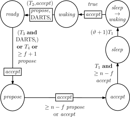
Figure 1: Basic cycle of node $i$ once the algorithm has stabilized.

The full algorithm makes use of a rather involved interplay between conditions on timeouts, states, and thresholds to converge to a safe state despite a limited number of faulty components. As our approach is thus difficult to present in bulk, we break it down into pieces. Moreover, to facilitate giving intuition about the key ideas of the algorithm, in this section we assume that there are $f<n/3$ faulty nodes, and the remaining $n-f$ nodes are non-faulty within $[0,\infty)$ (where of course the time $0$ is unknown to the nodes). We further assume that channels between non-faulty nodes (including loopback channels) are correct within $[0,\infty)$. We start by presenting the basic cycle that is repeated every pulse once a safe configuration is reached (see [fig:main_simple]Figure 1).

We employ graphical representations of the state machine of each node $i\in V$. States are represented by circles containing their names, while transition $(s,s^{\prime})\in\cal T$ is depicted as an arrow from $s$ to $s^{\prime}$. The guard $tr(s,s^{\prime})$ is written as a label next to the arrow, and the reset function’s value $re(s,s^{\prime})$ is depicted in a rectangular box on the arrow. To keep labels more simple we make use of some abbreviations. We write $T$ instead of $(T,s)$ if $s$ is the state which node $i$ leaves if the condition involving $(T,s)$ is satisfied. Threshold conditions like “ $\geq f+1$ $s$ ”, where $s\in\mathbb{S}$, abbreviate Boolean predicates that reach over all of node $i$’s memory flags $\operatorname{Mem}_{i,j,s}$, where $j\in V$, and are defined in a straightforward manner. If in such an expression we connect two states by “or”, e.g., “ $\geq n-f$ $s$ or $s^{\prime}$ ” for $s,s^{\prime}\in\mathbb{S}$, the summation considers flags of both types $s$ and $s^{\prime}$. Thus, such an expression is equivalent to $\sum_{j\in V}\max\{\operatorname{Mem}_{i,j,s},\operatorname{Mem}_{i,j,s^{\prime}}\}\geq f+1$. For any state $s\in\mathbb{S}$, the condition $S_{i,j}=s$, (respectively, $\neg(S_{i,j}=s)$) is written in short as “$j$ in $s$” (respectively, “$j$ not in $s$”). If $j=i$, we simply write “(not) in $s$”. We write “true” instead of a condition that is always true (like e.g. “(in $s$) or (not in $s$)” for an arbitrary state $s\in\mathbb{S}$). Finally, $re(\cdot,\cdot)$ always requires to reset all memory flags of certain types, hence we write e.g. propose if all flags $\operatorname{Mem}_{i,j,\emph{propose}}$ are to be reset.

We now briefly introduce the basic flow of the algorithm once it stabilizes, i.e., once all $n-f$ non-faulty nodes are well-synchronized. Recall that the remaining up to $f<n/3$ faulty nodes may produce arbitrary signals on their outgoing channels. A pulse is locally triggered by switching to state accept. Thus, assume that at some time all non-faulty nodes switch to state accept within a time window of $2d$, i.e., a valid pulse is generated. Supposing that $T_{1}\geq 3\vartheta d$, these nodes will observe, and thus memorize, each other and themselves in state accept before $T_{1}$ expires. This makes timeout $T_{1}$ the critical condition for switching to state sleep. From state sleep, they will switch to states $\emph{sleep}\rightarrow\emph{waking}$, waking, and finally ready, where the timeout $(T_{2},\emph{accept})$ is determining the time this takes, as it is considerably larger than $\vartheta(\vartheta+2)T_{1}$. The intermediate states serve the purpose of achieving stabilization, hence we leave them out for the moment. Note that upon switching to state ready, nodes reset their propose flags and $\mbox{\sc{darts}}_{i}$. Thus, they essentially ignore these signals between the most recent time they switched to propose before switching to accept and the subsequent time when they switch to ready. This ensures that nodes do not take into account outdated information for the decision when to switch to state propose. Hence, it is guaranteed that the first node switching from state ready to state propose again does so because $T_{4}$ expired or because $T_{3}$ expired and its darts memory flag is true. Due to the constraint $\min\{T_{3},T_{4}\}\geq\vartheta(T_{2}+4d)$, we are sure that all non-faulty nodes observe themselves in state ready before the first one switches to propose. Hence, no node deletes information about nodes that switch to propose  again after the previous pulse. The first non-faulty node that switches to state accept again cannot do so before it memorizes at least $n-f$ nodes in state propose, as the accept flags are reset upon switching to state propose. Therefore, at this time at least $n-2f\geq f+1$ non-faulty nodes are in state propose. Hence, the rule that nodes switch to propose if they memorize $f+1$ nodes in states propose will take effect, i.e., the remaining non-faulty nodes in state ready  switch to propose after less than $d$ time. Another $d$ time later all non-faulty nodes in state propose will have become aware of this and switch to state accept  as well, as the threshold of $n-f$ nodes in states propose or accept is reached. Thus the cycle is complete and the reasoning can be repeated inductively.

Clearly, for this line of argumentation to be valid, the algorithm could be simpler than stated in [fig:main_simple]Figure 1. We already mentioned that the motivation of having three intermediate states between accept and ready is to facilitate stabilization. Similarly, there is no need to make use of the accept  flags in the basic cycle at all; in fact, it adversely affects the constraints the timeouts need to satisfy for the above reasoning to be valid. However, the accept flags are much better suited for diagnostic purposes than the propose  flags, since nodes are expected to switch to accept in a small time window and remain in state accept for a small period of time only (for all our results, it is sufficient if $T_{1}=4\vartheta d$). Moreover, two different timeout conditions for switching from ready to propose are unnecessary for correct operation of the pulse synchronization routine. As discussed before, they are introduced in order to allow for a seamless coupling to the darts system. We elaborate on this in [sec:coupling]Section 7.

3.2 Main Algorithm

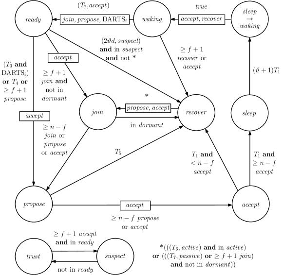
Figure 2: Overview of the core routine of node $i$’s self-stabilizing pulse algorithm.

We proceed by describing the main routine of the pulse algorithm in full. Alongside the main routine, several other state machines run concurrently and provide additional information to be used during recovery.

The main routine is graphically presented in [fig:main]Figure 2, together with a very simple second component whose sole purpose is to simplify the otherwise overloaded description of the main routine. Except for the states recover and join and additional resets of memory flags, the main routine is identical to the basic cycle. The purpose of the two additional states is the following: Nodes switch to state recover once they detect that something is wrong, that is, non-faulty nodes do not execute the basic cycle as outlined in [sec:basic_cycle]Section 3.1. This way, non-faulty nodes will not continue to confuse others by sending for example state signals propose or accept despite clearly being out-of-sync. There are various consistency checks that nodes perform during each execution of the basic cycle. The first one is that in order to switch from state accept to state sleep, non-faulty nodes need to memorize at least $n-f$ nodes in state accept. If this does not happen within $T_{1}$ time after switching to state accept, by the arguments given in [sec:basic_cycle]Section 3.1, they could not have entered state accept within $2d$ of each other. Therefore, something must be wrong and it is feasible to switch to state recover. Next, whenever a non-faulty node is in state waking, there should be no non-faulty nodes in states accept or recover. Considering that the node resets its accept and recover flags upon switching to waking, it should not memorize $f+1$ or more nodes in states accept or recover at a time when it observes itself in state waking. If it does, however, it again switches to state recover. Similarly, when in state ready, nodes expect others not to be in state accept for more than a short period of time, as a non-faulty node switching to accept should imply that every non-faulty node switches to propose and then to accept shortly thereafter. This is expressed by the second state machine comprising two states only. If a node is in state ready and memorizes $f+1$ nodes in state accept, it switches to suspect. Subsequently, if it remains in state ready until a timeout of $2\vartheta d$ expires, it will switch to state recover. Last but not least, during a synchronized execution of the basic cycle, no non-faulty node may be in state propose for more than a certain amount of time before switching to state accept. Therefore, nodes will switch from propose to recover when timeout $T_{5}$ expires.

Nodes can join the basic cycle again via the second new state, called join. Since the Byzantine nodes may “play nice” towards $n-2f$ or more nodes still executing the basic cycle, making them believe that system operation continues as usual, it must be possible to join the basic cycle again without having a majority of nodes in state recover. On the other hand, it is crucial that this happens in a sufficiently well-synchronized manner, as otherwise nodes could drop out again because the various checks of consistency detect an erroneous execution of the basic cycle.

In part, this issue is solved by an additional agreement step. In order to enter the basic cycle again, nodes need to memorize $n-f$ nodes in states join (the respective nodes detected an inconsistency), propose (these nodes continued to execute the basic cycle), or accept (there are executions where nodes reset their propose flags because of switching to join when other nodes already switched to accept). Since there are thresholds of $f+1$ nodes memorized in state join both for leaving state recover and switching from ready to join, all nodes will follow the first one switching from join to propose quickly, just as with the switch from propose to accept in an ordinary execution of the basic cycle. However, it is decisive that all nodes are in states that permit to participate in this agreement step in order to guarantee success of this approach.

As a result, still a certain degree of synchronization needs to be established beforehand, both among nodes that still execute the basic cycle and those that do not. For instance, if at the point in time when a majority of nodes and channels become non-faulty, some nodes already memorize nodes in join that are not, they may switch to state join and subsequently propose prematurely, causing others to have inconsistent memory flags as well. Again, Byzantine faults may sustain this amiss configuration of the system indefinitely.

So why did we put so much effort in “shifting” the focus to this part of the algorithm? The key advantage is that nodes outside the basic cycle may take into account less reliable information for stabilization purposes. They may take the risk of metastable upsets (as we know it is impossible to avoid these during the stabilization process, anyway) and make use of randomization.

In fact, to make the above scheme work, it is sufficient that all non-faulty nodes agree on a so called resynchronization point (formally defined later on), that is, a point in time at which nodes reset the memory flags for states join and $\emph{sleep}\rightarrow\emph{waking}$ as well as certain timeouts, while guaranteeing that no node is in these states close to the respective reset times. Except for state $\emph{sleep}\rightarrow\emph{waking}$, all of these timeouts, memory flags, etc. are not part of the basic cycle at all, thus nodes may enforce consistent values for them when they agree on such a resynchronization point.

Conveniently, the use of randomization also ensures that it is quite unlikely that nodes are in state $\emph{sleep}\rightarrow\emph{waking}$ close to a resynchronization point, as the consistency check of having to memorize $n-f$ nodes in state accept in order to switch to state sleep guarantees that the time windows during which non-faulty nodes may switch to sleep make up a small fraction of all times only.

Consequently, the remaining components of the algorithm deal with agreeing on resynchronization points and utilizing this information in an appropriate way to ensure stabilization of the main routine. We describe this connection to the main routine first. It is done by another, quite simple state machine, which runs in parallel alongside the core routine. It is depicted in [fig:extended]Figure 3.

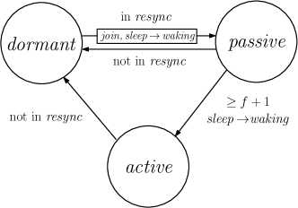
Figure 3: Extension of node $i$’s core routine.

Its purpose is to reset memory flags in a consistent way and to determine when a node is permitted to switch to join. In general, a resynchronization point (locally observed by switching to state resync, which is introduced later) triggers the reset of the join and $\emph{sleep}\rightarrow\emph{waking}$ flags. If there are still nodes executing the basic cycle, a node may become aware of it by observing $f+1$ nodes in state $\emph{sleep}\rightarrow\emph{waking}$ at some time. In this case it switches from the state passive, which it entered at the point in time when it locally observed the resynchronization point, to the state active, which enables an earlier transition to state join. This is expressed by the rather involved transition rule $tr(\emph{recover},\emph{join})$: $T_{6}$ is much smaller than $T_{7}$, but $T_{6}$ is of no concern until the node switches to state active and resets $T_{6}$.

It remains to explain how nodes agree on resynchronization points.

3.3 Resynchronization Algorithm

The resynchronization routine is specified in [fig:resync]Figure 4 as well. It is a lower layer that the core routine uses for stabilization purposes only. It provides some synchronization that is very similar to that of a pulse, except that such “weak pulses” occur at random times, and may be generated inconsistently after the algorithm as a whole has stabilized. Since the main routine operates independently of the resynchronization routine once the system has stabilized, we can afford the weaker guarantees of the routine: If it succeeds in generating a “good” resynchronization point merely once, the main routine will stabilize deterministically.

Definition 3.1 (Resynchronization Points).

Given $W\subseteq V$, time $t$ is a $W$-resynchronization point iff each node in $W$ switches to state $\emph{supp}\rightarrow\emph{resync}$ in the time interval $(t,t+2d)$.

Definition 3.2 (Good Resynchronization Points).

A $W$-resynchronization point is called good if no node from $W$ switches to state sleep during $(t-(\vartheta+3)T_{1},t)$ and no node is in state join during $[t-T_{1}-d,t+4d)$.

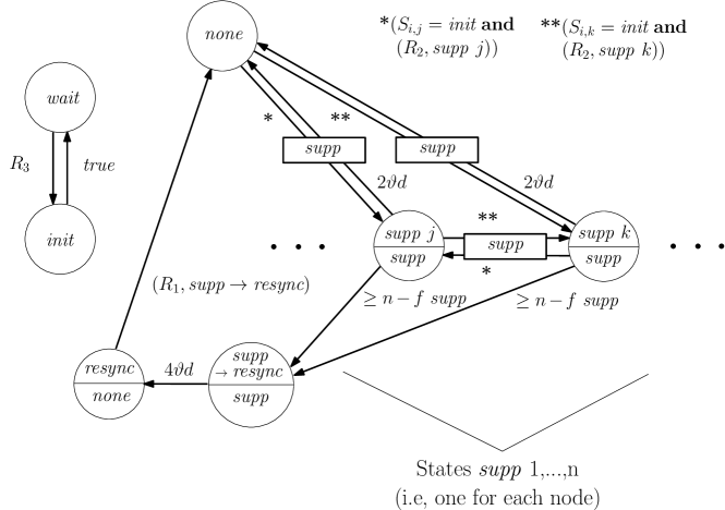
Figure 4: Resynchronization algorithm, comprising two state machines executed in parallel at node $i$.

In order to clarify that despite having a linear number of states ($\emph{supp}_{1},\ldots,\emph{supp}_{n}$), this part of the algorithm can be implemented using $2$-bit communication channels between state machines only, we generalize our description of state machines as follows. If a state is depicted as a circle separated into an upper and a lower part, the upper part denotes the local state, while the lower part indicates the signal state to which it is mapped. A node’s memory flags then store the respective signal states only, i.e., remote nodes do not distinguish between states that share the same signal. Clearly, such a machine can be simulated by a machine as introduced in the model section. The advantage is that such a mapping can be used to reduce the number of transmitted state bits; for the resynchronization routine given in [fig:resync]Figure 4, we merely need two bits (init/wait and none/supp) instead of $\lceil\log(n+3)\rceil+1$ bits.

The basic idea behind the resynchronization algorithm is the following: Every now and then, nodes will try to initiate agreement on a resynchronization point. This is the purpose of the small state machine on the left in [fig:resync]Figure 4. Recalling that the transition condition “true” simply means that the node switches to state wait again as soon as it observes itself in state init, it is easy to see that it does nothing else than creating an init signal as soon as $R_{3}$ expires and resetting $R_{3}$ again as quickly as possible. As the time when a node switches to init is determined by the randomized timeout $R_{3}$ distributed over a large interval (cf. Equality (11)) only, it is impossible to predict when it will expire, even with full knowledge of the execution up to the current point in time. Note that the complete independence of this part of node $i$’s state from the remaining protocol implies that faulty nodes are not able to influence the respective times by any means.

Consider now the state machine displayed on the right of [fig:resync]Figure 4. To understand how the routine is intended to work, assume that at the time $t$ when a non-faulty node $i$ switches to state init, all non-faulty nodes are not in any of the states $\emph{supp}\rightarrow\emph{resync}$, resync, or supp $i$, and at all non-faulty nodes the timeout $(R_{2},\emph{supp}~{}i)$ has expired. Then, no matter what the signals from faulty nodes or on faulty channels are, all non-faulty nodes will be in one of the states supp $j$, $j\in V$, or $\emph{supp}\rightarrow\emph{resync}$ at time $t+d$. Hence, they will observe each other (and themselves) in one of these states at some time smaller than $t+2d$. These statements follow from the various timeout conditions of at least $2\vartheta d$ and the fact that observing node $i$ in state init will make nodes switch to state supp $i$ if in none or supp $j$, $j\neq i$. Hence, all of them will switch to state $\emph{supp}\rightarrow\emph{resync}$ during $(t,t+2d)$, i.e., $t$ is a resynchronization point. Since $t$ follows a random distribution that is independent of the remaining algorithm and, as mentioned earlier, most of the times nodes cannot switch to state sleep and it is easy to deal with the condition on join states, there is a large probability that $t$ is a good resynchronization point. Note that timeout $R_{1}$ makes sure that no non-faulty node will switch to $\emph{supp}\rightarrow\emph{resync}$ again anytime soon, leaving sufficient time for the main routine to stabilize.

The scenario we just described relies on the fact that at time $t$ no node is in state $\emph{supp}\rightarrow\emph{resync}$ or state resync. We will choose $R_{2}\gg R_{1}$, implying that $R_{2}+3d$ time after a node switched to state init all nodes have “forgotten” about this, i.e., $(R_{2},\emph{supp}~{}i)$ is expired and they switched back to state none  (unless other init signals interfered). Thus, in the absence of Byzantine faults, the above requirement is easily achieved with a large probability by choosing $R_{3}$ as a uniform distribution over some interval $[R_{2}+3d,R_{2}+\Theta(nR_{1})]$: Other nodes will switch to init $\mathcal{O}(n)$ times during this interval, each time “blocking” other nodes for at most $\mathcal{O}(R_{1})$ time. If the random choice picks any other point in time during this interval, a resynchronization point occurs. Even if the clock speed of the clock driving $R_{3}$ is manipulated in a worst-case manner (affecting the density of the probability distribution with respect to real time by a factor of at most $\vartheta$), we can just increase the size of the interval to account for this.

However, what happens if only some of the nodes receive an init signal due to faulty channels or nodes? If the same holds for some of the subsequent supp signals, it might happen that only a fraction of the nodes reaches the threshold for switching to state $\emph{supp}\rightarrow\emph{resync}$, resulting in an inconsistent reset of flags and timeouts across the system. Until the respective nodes switch to state none again, they will not support a resynchronization point again, i.e., about $R_{1}$ time is “lost”. This issue is the reason for the agreement step and the timeouts $(R_{2},\emph{supp}~{}j)$. In order for any node to switch to state $\emph{supp}\rightarrow\emph{resync}$, there must be at least $n-2f\geq f+1$ non-faulty nodes supporting this. Hence, all of these nodes recently switched to a state supp $j$ for some $j\in V$, resetting $(R_{2},\emph{supp}~{}j)$. Until these timeouts expire, $f+1\in\Omega(n)$ non-faulty nodes will ignore init signals on the respective channels. Since there are $\mathcal{O}(n^{2})$ channels, it is possible to choose $R_{2}\in\mathcal{O}(nR_{1})$ such that this may happen at most $\mathcal{O}(n)$ times in $\mathcal{O}(n)$ time. Playing with constants, we can pick $R_{3}\in\mathcal{O}(n)$ maintaining that still a constant fraction of the times are “good” in the sense that $R_{3}$ expiring at a non-faulty node will result in a good resynchronization point.

3.4 Timeout Constraints

[cond:timeout_bounds]Condition 3.3 summarizes the constraints we require on the timeouts for the core routine and the resynchronization algorithm to act and interact as intended.

Condition 3.3 (Timeout Constraints).

Define

$$\lambda:=\sqrt{\frac{25\vartheta-9}{25\vartheta}}\in\left(\frac{4}{5},1\right),$$ (1)

$\Delta_{g}:=(\vartheta+3)T_{1}$, $\Delta_{s}:=T_{2}/\vartheta-2T_{1}-d$, $\delta_{s}:=2T_{1}+3d$, and $\tilde{\delta}_{s}:=(\vartheta+2-1/\vartheta)T_{1}+4d$. The timeouts need to satisfy the constraints

$$T_{1} \geq \vartheta 4d$$ (2)

$$T_{2} \geq \vartheta\max\left\{T_{1}+\Delta_{g}-(4\vartheta^{2}+16\vartheta+5)d,\left(3\vartheta+1-\frac{1}{\vartheta}\right)T_{1}+T_{5}\right\}$$ (3)

$$T_{3} \geq \max\left\{(\vartheta-1)T_{2}+\vartheta(2T_{1}+(2\vartheta+4)d),(2\vartheta^{2}+3\vartheta-1)T_{1}-T_{2}+\vartheta(T_{6}+5d)\right\}$$ (4)

$$T_{4} \geq T_{3}$$ (5)

$$T_{5} \geq \max\left\{\vartheta(T_{4}+7d)-T_{3}+(\vartheta-1)T_{2},(\vartheta^{2}+\vartheta-2)T_{1}+\vartheta(T_{2}+T_{4}+9d)-T_{6}\right\}$$ (6)

$$T_{6} \geq \vartheta\left(\tilde{\delta}_{s}-\left(1-\frac{1}{\vartheta}\right)T_{1}+T_{2}+2d\right)>\vartheta\Delta_{s}$$ (7)

$$T_{7} \geq \vartheta(T_{2}+T_{4}+T_{5}+\Delta_{s}+\tilde{\delta}_{s}-\Delta_{g}+d)+T_{6}-4d$$ (8)

$$R_{1} \geq \vartheta\max\left\{T_{7}+(4\vartheta+8)d,\left(2\vartheta+4-\frac{3}{\vartheta}\right)T_{1}+2T_{4}+T_{5}-\Delta_{s}-\Delta_{g}+17d\right\}$$ (9)

$$R_{2} \geq \frac{2\vartheta(R_{1}+(\vartheta+2)T_{1}+T_{2}/\vartheta+(8\vartheta+9)d)(n-f)}{1-\lambda}$$ (10)

$$R_{3} = \mbox{uniformly distributed random variable on }\left[\vartheta(R_{2}+3d),\vartheta(R_{2}+3d)+8(1-\lambda)R_{2}\right]$$ (11)

$$\lambda \leq \frac{\Delta_{s}-\Delta_{g}-\delta_{s}}{\Delta_{s}}.$$ (12)

We need to show for which values of $\vartheta$ this system can be solved. Furthermore, we would like to allow for the largest possible drift of DARTS clocks, which necessitates to maximize the ratio $(T_{2}+T_{4})/(\vartheta(T_{2}+T_{3}+4d))$, that is, the minimal gap between pulses provided that the states of the darts signals are zero divided by the maximal time it takes nodes to observe themselves in state ready with $T_{3}$ expired after a pulse (as then they will respond to $\mbox{\sc{darts}}_{i}$ switching to one).

Lemma 3.4.

Define $\vartheta_{\max}\approx 1.247$ as the positive solution of $2\vartheta+1=\vartheta^{3}+\vartheta^{2}$. Given that $\vartheta<\vartheta_{\max}$, [cond:timeout_bounds]Condition 3.3 can be satisfied with $T_{1},\ldots,T_{7},R_{1}\in\mathcal{O}(1)$ and $R_{2}\in\mathcal{O}(n)$. The ratio

$$\frac{(T_{2}+T_{4})/\vartheta}{T_{2}+T_{3}+4d}$$

can be made larger than any constant smaller than

$$\frac{\vartheta^{3}+2\vartheta+1}{2\vartheta^{4}+\vartheta^{3}}.$$

Proof.

First, we identify several redundant inequalities in the system. We have that

$$\left(2\vartheta+2-\frac{1}{\vartheta}\right)T_{1}+T_{5} \stackrel{{\scriptstyle\eqref{eq:T_5}}}{{>}} 3\vartheta T_{1}+T_{2}+T_{4}-T_{6}$$

$$\stackrel{{\scriptstyle(\ref{eq:T_3},\ref{eq:T_4})}}{{>}} 7\vartheta T_{1}$$

$$> T_{1}+\Delta_{g}-(4\vartheta^{2}+16\vartheta+5)d,$$

i.e., the left term in the maximum in [eq:T_2]Inequality (3) is redundant. The same holds true for the left terms in the maxima in [eq:T_3]Inequality (4) and [eq:T_5]Inequality (6), since

$$(2\vartheta^{2}+3\vartheta-1)T_{1}-T_{2}+\vartheta(T_{6}+5d) \stackrel{{\scriptstyle\eqref{eq:T_6}}}{{>}} 3\vartheta T_{1}+(\vartheta-1)T_{2}+4d$$

$$\stackrel{{\scriptstyle\eqref{eq:T_1}}}{{>}} (\vartheta-1)T_{2}+\vartheta(2T_{1}+(2\vartheta+4)d)$$

and

$$\vartheta(T_{4}+7d)-T_{3}+(\vartheta-1)T_{2} \stackrel{{\scriptstyle\eqref{eq:T_3}}}{{<}} \vartheta(T_{2}+T_{4}-T_{6}+7d)$$

$$< (\vartheta^{2}+\vartheta-2)T_{1}+\vartheta(T_{2}+T_{4}+9d)-T_{6}.$$

Finally, we can eliminate the right term in the maximum in [eq:R_1]Inequality (9) from the system, as

$$T_{7}+(4\vartheta+8)d \stackrel{{\scriptstyle\eqref{eq:T_7}}}{{>}} T_{2}+T_{4}+T_{5}+T_{6}+2\tilde{\delta}_{s}-\Delta_{g}+13d$$

$$\stackrel{{\scriptstyle\eqref{eq:T_2}}}{{>}} \left(2\vartheta+4-\frac{3}{\vartheta}\right)T_{1}+T_{4}+2T_{5}+T_{6}-\Delta_{g}+17d$$

$$\stackrel{{\scriptstyle\eqref{eq:T_5}}}{{>}} \left(2\vartheta+4-\frac{3}{\vartheta}\right)T_{1}+T_{2}+2T_{4}+T_{5}-\Delta_{g}+17d.$$

Next, it is not difficult to see that the right hand sides of all inequalities are strictly increasing in $T_{1}$ (except for [eq:lambda]Inequality (12), whose right hand side decreases with $T_{1}$), implying that w.l.o.g. we may set $T_{1}:=4\vartheta d$. Similarly, we demand that [eq:T_7]Inequality (8), [eq:R_1]Inequality (9), and [eq:R_2]Inequality (10) are satisfied with equality, i.e.,

$$T_{7} = \vartheta(T_{2}+T_{4}+T_{5})+T_{6}-(4\vartheta^{2}+4)d$$

$$R_{1} = \vartheta T_{7}+(4\vartheta^{2}+8\vartheta)d$$

$$R_{2} = \frac{2\vartheta(R_{1}+T_{2}/\vartheta+(4\vartheta^{2}+16\vartheta+9)d)(n-f)}{1-\lambda}$$

$$R_{3} = \mbox{uniformly distributed random variable on }\left[\vartheta(R_{2}+3d),\vartheta(R_{2}+3d)+8(1-\lambda)R_{2}\right].$$

We set $T_{4}:=\alpha T_{3}$ for a parameter

$$\alpha\in\left[1,\frac{2\vartheta+1}{\vartheta^{3}+\vartheta^{2}}\right),$$

implying that [eq:T_4]Inequality (5) holds by definition. The remaining simpler system is as follows.

$$T_{2} \geq (8\vartheta^{3}+8\vartheta^{2}-4\vartheta)d+\vartheta T_{5}$$ (13)

$$T_{3} \geq (8\vartheta^{3}+12\vartheta^{2}+\vartheta)d-T_{2}+\vartheta T_{6}$$ (14)

$$T_{5} \geq (4\vartheta^{3}+4\vartheta^{2}+\vartheta)d+\vartheta(T_{2}+\alpha T_{3})-T_{6}$$ (15)

$$T_{6} \geq (4\vartheta^{2}+6\vartheta-4)d+T_{2}$$ (16)

$$\sqrt{\frac{25\vartheta-9}{25\vartheta}} \leq \frac{T_{2}/\vartheta-(4\vartheta^{2}+28\vartheta+4)d}{T_{2}/\vartheta-(8\vartheta+1)d}.$$

Note the above equalities do not affect this system and can be resolved iteratively once the other variables are fixed. We observe that the right hand side of [eq:T_2_simple]Inequality (13) is increasing in $T_{5}$, the right hand side of [eq:T_5_simple]Inequality (15) is increasing in $T_{3}$, and neither $T_{3}$ nor $T_{5}$ are present in any further inequalities. Hence, we rule that [eq:T_3_simple]Inequality (14) and [eq:T_5_simple]Inequality (15) shall be satisfied with equality, i.e.,

$$T_{3} = (8\vartheta^{3}+12\vartheta^{2}+\vartheta)d-T_{2}+\vartheta T_{6}$$

$$T_{5} = (\alpha(8\vartheta^{4}+12\vartheta^{3}+\vartheta^{2})+(4\vartheta^{3}+4\vartheta^{2}+\vartheta))d-(\vartheta\alpha-1)T_{2}+(\vartheta^{2}\alpha-1)T_{6}$$

and arrive at the subsystem

$$T_{2} \geq \frac{(\alpha(8\vartheta^{5}+12\vartheta^{4}+\vartheta^{3})+(4\vartheta^{4}+12\vartheta^{3}+9\vartheta^{2}-4\vartheta))d+(\vartheta^{3}\alpha-\vartheta)T_{6}}{1+\vartheta-\vartheta^{2}\alpha}$$ (17)

$$T_{6} \geq (4\vartheta^{2}+6\vartheta-4)d+T_{2}$$

$$T_{2} \geq \frac{(4\vartheta^{3}+20\vartheta^{2}+3\vartheta)d}{1-\sqrt{(25\vartheta-9)/(25\vartheta)}},$$

where we used that $1+\vartheta-\vartheta^{2}\alpha>0$. Now we can see that [eq:T_2_simpler]Inequality (17) is also increasing in $T_{6}$, set

$$T_{6}:=(4\vartheta^{2}+6\vartheta-4)d+T_{2},$$

and obtain

$$T_{2} \geq \frac{(\alpha(12\vartheta^{5}+18\vartheta^{4}-3\vartheta^{3})+(4\vartheta^{4}+8\vartheta^{3}+3\vartheta^{2}))d}{1+2\vartheta-(\vartheta^{3}+\vartheta^{2})\alpha}$$ (18)

$$T_{2} \geq \frac{25(1+\sqrt{(25\vartheta-9)/(25\vartheta)})(4\vartheta^{4}+20\vartheta^{3}+3\vartheta^{2})d}{9},$$ (19)

exploiting that $1+2\vartheta-(\vartheta^{3}+\vartheta^{2})\alpha>0$.

Since $\alpha$ and thus $\vartheta$ are constantly bounded (and we treat $d$ as constant as well), we have a feasible solution for $T_{2}\in\mathcal{O}(1)$ (considering asymptotic with respect to $n$). Resolving the equalities we derived for the other variables, we see that $T_{1},\ldots,T_{7},R_{1}\in\mathcal{O}(1)$ and $R_{2}\in\mathcal{O}(n)$ as claimed.

It remains to determine the maximal ratio $(T_{2}+T_{4})/(\vartheta(T_{2}+T_{3}+4d))=(T_{2}+\alpha T_{3})/(\vartheta(T_{2}+T_{3}+4d))$ we can ensure. Obviously, for any value of $\alpha$, fixing either $T_{2}$ or $T_{3}$ implies that we want to minimize $T_{2}$ or maximize $T_{3}$, respectively. Have a look at Inequalities (13)–(16) again. The solution we constructed minimized $T_{3}$ and subsequently $T_{2}$, parametrized by feasible values of $\alpha$. Increase now $T_{3}$ by $x\in\mathbb{R}^{+}$ in [eq:T_3_simple]Inequality (14). Consequently, we may increase $T_{6}$ in [eq:T_6_simple]Inequality (16) by $x/\vartheta$ compared to our previous solution (where we minimized all inequalities). Hence, we need to increase $T_{5}$ by $(\vartheta\alpha-1/\vartheta)x$ according to [eq:T_5_simple]Inequality (15), and finally $T_{2}$ by $\vartheta(\vartheta\alpha-1/\vartheta)x$. Thus, for any feasible $\alpha$ and any $\varepsilon>0$, we can achieve that $T_{2}\leq(\vartheta^{2}\alpha-1+\varepsilon)T_{3}$ if we just choose $x$ large enough. We conclude that we can get arbitrarily close to the ratio

$$\frac{(\alpha+(\vartheta^{2}\alpha-1))T_{3}}{\vartheta(1+(\vartheta^{2}\alpha-1))T_{3}}=\frac{\vartheta^{2}\alpha+\alpha-1}{\vartheta^{3}\alpha}.$$

Inserting the supremum of admissible values for $\alpha$, this expression becomes

$$\frac{(2\vartheta+1)(\vartheta^{2}+1)-(\vartheta^{3}+\vartheta^{2})}{\vartheta^{3}(2\vartheta+1)}=\frac{\vartheta^{3}+2\vartheta+1}{2\vartheta^{4}+\vartheta^{3}}.$$

This shows the last claim of the lemma, concluding the proof. ∎

4 Analysis

In this section we derive skew bounds $\Sigma$, as well as accuracy bounds $T^{-},T^{+}$, such that the presented protocol is a $(W,E)$-stabilizing pulse synchronization protocol, for proper choices of the set of nodes $W$ and the set of channels $E$, with skew $\Sigma$ and accuracy bounds $T^{-},T^{+}$ that stabilizes within time $T(k)\in\mathcal{O}(kn)$ with probability $1-1/2^{k(n-f)}$, for any $k\in\mathbb{N}$.

To start our analysis, we need to define the basic requirements for stabilization. Essentially, we need that a majority of nodes is non-faulty and the channels between them are correct. However, the first part of the stabilization process is simply that nodes “forget” about past events that are captured by their timeouts. Therefore, we demand that these nodes indeed have been non-faulty for a time period that is sufficiently large to ensure that all timeouts have been reset at least once after the considered set of nodes became non-faulty.

Definition 4.1 (Coherent States).

The subset of nodes $W\subseteq V$ is called coherent during the time interval $[t^{-},t^{+}]$, iff during $[t^{-}-(\vartheta(R_{2}+3d)+8(1-\lambda)R_{2})-d,t^{+}]$ all nodes $i\in W$ are non-faulty, and all channels $S_{i,j}$, $i,j\in W$, are correct.

We will show that if a coherent set of at least $n-f$ nodes fires a pulse, i.e., switches to accept in a tight synchrony, this set will generate pulses deterministically and with controlled frequency, as long the set remains coherent. This motivates the following definitions.

Definition 4.2 (Stabilization Points).

We call $t$ a $W$-stabilization point (quasi-stabilization point) iff all nodes $i\in W$ switch to accept during $[t,t+2d)$ $([t,t+3d))$.

Throughout this section, we assume the set of coherent nodes $W$ with $|W|\geq n-f$ to be fixed and consider all nodes in and channels originating from $V\setminus W$ as (potentially) faulty. As all our statements refer to nodes in $W$, we will typically omit the word “non-faulty” when referring to the behaviour or states of nodes in $W$, and “all nodes” is short for “all nodes in $W$”. Note, however, that we will still clearly distinguish between channels originating at faulty and non-faulty nodes, respectively, to nodes in $W$.

As a first step, we observe that at times when $W$ is coherent, indeed all nodes reset their timeouts, basing the respective state transition on proper perception of nodes in $W$.

Lemma 4.3.

If the system is coherent during the time interval $[t^{-},t^{+}]$, any (randomized) timeout $(T,s)$ of any node $i\in W$ expiring at a time $t\in[t^{-},t^{+}]$ has been reset at least once since time $t^{-}-(\vartheta(R_{2}+3d)+8(1-\lambda)R_{2})$. If $t^{\prime}$ denotes the time when such a reset occurred, for any $j\in W$ it holds that $S_{i,j}(t^{\prime})=S_{j}(\tau_{j,i}^{-1}(t^{\prime}))$, i.e., at time $t^{\prime}$, $i$ observes $j$ in a state $j$ attained when it was non-faulty.

Proof.

According to [cond:timeout_bounds]Condition 3.3, the largest possible value of any (randomized) timeout is $\vartheta(R_{2}+3d)+8(1-\lambda)R_{2}$. Hence, any timeout that is in state $1$ at a time smaller than $t^{-}-(\vartheta(R_{2}+3d)+8(1-\lambda)R_{2})$ expires before time $t_{1}$ or is reset at least once. As by the definition of coherency all nodes in $W$ are non-faulty and all channels between such nodes are correct during $[t^{-}-(\vartheta(R_{2}+3d)+8(1-\lambda)R_{2})-d,t^{+}]$, this implies the statement of the lemma. ∎

Phrased informally, any corruption of timeout and channel states eventually ceases, as correct timeouts expire and correct links remember no events that lie $d$ or more time in the past. Proper cleaning of the memory flags is more complicated and will be explained further down the road. Throughout this section, we will assume for the sake of simplicity that the system is coherent at all times and use this lemma implicitly, e.g. we will always assume that nodes from $W$ will observe all other nodes from $W$ in states that they indeed had less than $d$ time ago, expiring of randomized timeouts at non-faulty nodes cannot be predicted accurately, etc. We will discuss more general settings in [sec:generalizations]Section 5.

We proceed by showing that once all nodes in $W$ switch to accept in a short period of time, i.e., a $W$-quasi-stabilization point is reached, the algorithm guarantees that synchronized pulses are generated deterministically with a frequency that is bounded both from above and below.

Theorem 4.4.

Suppose $t$ is a $W$-quasi-stabilization point. Then

• all nodes in $W$ switch to accept exactly once within $[t,t+3d)$, and do not leave accept until $t+4d$, and

• there will be a $W$-stabilization point $t^{\prime}\in(t+(T_{2}+T_{3})/\vartheta,t+T_{2}+T_{4}+5d)$ satisfying that no node in $W$ switches to accept in the time interval $[t+3d,t^{\prime})$ and that

• each node $i$’s, $i\in W$, core state machine ([fig:main_simple]Figure 1) is metastability-free during $[t+4d,t^{\prime}+4d)$.

Proof.

Proof of (i): Due to [eq:T_1]Inequality (2), a node does not leave the state accept earlier than $T_{1}/\vartheta\geq 4d$ time after switching to it. Thus, no node can switch to accept twice during $[t,t+3d)$. By definition of a quasi-stabilization point, every node does switch to accept in the interval $[t,t+3d)\subset[t,t+T_{1}/\vartheta)$. This proves Statement (i).

Proof of (ii): For each $i\in W$, let $t_{i}\in[t,t+3d)$ be the time when $i$ switches to accept. By (i) $t_{i}$ is well-defined. Further let $t^{\prime}_{i}$ be the infimum of times in $(t_{i},\infty)$ when $i$ switches to recover, join, or propose. In the following, denote by $i\in W$ a node with minimal $t^{\prime}_{i}$.

We will show that all nodes switch to propose via states sleep, $\emph{sleep}\rightarrow\emph{waking}$, waking, and ready in the presented order. By (i) nodes do not leave accept before $t+4d$. Thus at time $t+4d$, each node in $W$ is in state accept and observes each other node in $W$ in accept. Hence, each node in $W$ memorizes each other node in $W$ in accept at time $t+4d$. For each node $j\in W$, let $t_{j,s}$ be the time node $j$’s timeout $T_{1}$ expires first after $t_{j}$. Then $t_{j,s}\in(t_{j}+T_{1}/\vartheta,t_{j}+T_{1}+d)$. Since $|W|\geq n-f$, each node $j$ switches to state sleep at time $t_{j,s}$. Hence, by time $t+T_{1}+4d$, no node will be observed in state accept anymore (until the time when it switches to accept again).

When a node $j\in W$ switches to state waking at the minimal time $t_{w}$ larger than $t_{j}$, it does not do so earlier than at time $t+T_{1}/\vartheta+(1+1/\vartheta)T_{1}=t+(1+2/\vartheta)T_{1}>t+T_{1}+5d$. This implies that all nodes in $W$ have already left accept at least $d$ time ago, since they switched to it at their respective times $t_{j}<t+T_{1}+4d$. Moreover, they cannot switch to accept again until $t_{i}^{\prime}$ as it is minimal and nodes need to switch to propose  before switching to accept. Hence, nodes in $W$ are not observed in state accept during $(t+T_{1}+5d,t_{i}^{\prime}]$, in particular not by node $j$. Furthermore, nodes in $W$ are not observed in state recover during $(t_{w}-d,t_{i}^{\prime}]$. As it resets its accept and recover flags upon switching to waking, $j$ will hence neither switch from waking to recover nor from trust to suspect during $(t_{w},t_{i}^{\prime}]$, and thus also not from ready to recover.

Now consider node $i$. By the previous observation, it will not switch from waking to recover, but to ready, following the basic cycle. Consequently, it must wait for timeout $T_{2}$ to expire, i.e., cannot switch to ready earlier than at time $t+T_{2}/\vartheta$. As nodes in $W$ clear their join flags upon switching to state ready, by definition of $t_{i}^{\prime}$ node $i$ cannot switch from ready to join, but has to switch to propose. Again, by definition of $i$, it cannot do so before timeouts $T_{3}$ or $T_{4}$ expire, i.e., before time

$$t+\frac{T_{2}}{\vartheta}+\frac{\min\{T_{3},T_{4}\}}{\vartheta}\stackrel{{\scriptstyle\eqref{eq:T_4}}}{{=}}t+\frac{T_{2}+T_{3}}{\vartheta}\stackrel{{\scriptstyle\eqref{eq:T_3}}}{{>}}t+T_{2}+5d.$$ (20)

All other nodes in $W$ will switch to waking, and for the first time after $t_{j}$, observe themselves in state waking at a time within $(t+T_{1}+4d,t+T_{1}(2+\vartheta)+7d)$. Recall that unless they memorize at least $f+1$ nodes in accept or recover while being in state waking, they will all switch to state ready by time

$$\max\{t+T_{2}+4d,t+(\vartheta+2)T_{1}+7d\}\stackrel{{\scriptstyle\eqref{eq:T_2}}}{{=}}t+T_{2}+4d.$$ (21)

As we just showed that $t_{i}^{\prime}>t+T_{2}+5d$, this implies that at time $t+T_{2}+5d$ all nodes are observed in state ready, and none of them leaves before time $t_{i}^{\prime}$.

Now choose $t^{\prime}$ to be the infimum of times from $(t+(T_{2}+T_{3})/\vartheta,t+T_{2}+T_{4}+4d]$ when a node in $W$ switches to state accept. Because of [eq:low]Inequality (20), $t^{\prime}$ is the first time any node $j\in W$ may switch to accept again after its respective time $t_{j}$. We will next show that no node $j\in W$ can switch to recover within $[t_{j},t^{\prime}+2d]$. Since at time $t_{i}^{\prime}$ node $j$ does not memorize other nodes from $W$ in state accept, it will also not do so during $[t_{i}^{\prime},t^{\prime}]$. Hence, it cannot switch from ready to recover during $[t_{i}^{\prime},t^{\prime}+2d]$ since it cannot be in state suspect during $[t_{i}^{\prime},t^{\prime}]$. By [eq:low]Inequality (20), $j$ cannot switch to propose within $[t_{j},t+(T_{2}+T_{3})/\vartheta)$, and thus its timeout $T_{5}$ cannot expire until time

$$t+\frac{T_{2}+T_{3}+T_{5}}{\vartheta}\stackrel{{\scriptstyle\eqref{eq:T_5}}}{{\geq}}t+T_{2}+T_{4}+7d\geq t^{\prime}+3d,$$ (22)

making it impossible for $j$ to switch from propose to recover at a time within $[t_{j},t^{\prime}+3d]$. What is more, a node from $W$ that switches to accept must stay there for at least $T_{1}/\vartheta>3d$ time. Thus, by definition of $t^{\prime}$, no node $j\in W$ can switch from accept to recover at a time within $[t_{j},t^{\prime}+3d]$. Hence, no node $j\in W$ can switch to state recover after $t_{j}$, but earlier than time $t^{\prime}+2d$. As nodes reset their join flags upon switching to state ready, it follows that no node in $W$ can switch to other states than propose or accept  during $[t+T_{2}+4d,t^{\prime}+2d]$. In particular, no node in $W$ resets its propose flags during $[t+T_{2}+5d,t^{\prime}+2d]\supset[t_{i}^{\prime},t^{\prime}+2d]$.

If at time $t^{\prime}$ a node in $W$ switches to state accept, $n-2f\geq f+1$ of its propose flags corresponding to nodes in $W$ are true, i.e., in state $1$. As the node reset its propose flags at the most recent time when it switched to ready and no nodes from $W$ have been observed in propose between this time and $t_{i}^{\prime}$, it holds that $f+1$ nodes in $W$ switched to state propose during $[t_{i}^{\prime},t^{\prime})$. Since we established that no node resets its propose flags during $[t_{i}^{\prime},t^{\prime}+2d]$, it follows that all nodes are in state propose by time $t^{\prime}+d$. Consequently, all nodes in $W$ will observe all nodes in $W$ in state propose  before time $t^{\prime}+2d$ and switch to accept, i.e., $t^{\prime}\in(t+(T_{2}+T_{3})/\vartheta,t+T_{2}+T_{4}+4d)$ is a stabilization point. Statement (ii) follows.

On the other hand, if at time $t^{\prime}$ no node in $W$ switches to state accept, it follows that $t^{\prime}=t+T_{2}+T_{4}+4d$. As all nodes observe themselves in state ready  by time $t+T_{2}+5d$, they switch to propose before time $t+T_{2}+T_{4}+5d=t^{\prime}+d$ because $T_{4}$ expired. By the same reasoning as in the previous case, they switch to accept before time $t^{\prime}+2d$, i.e., Statement (ii) holds as well.

Proof of (iii): We have shown that within $[t_{j},t^{\prime}+2d]$, any node $j\in W$ switches to states along the basic cycle only. Moreover, such nodes switch to accept at some time in $[t^{\prime},t^{\prime}+2d]$. Since $T_{1}\geq 4\vartheta d$, this implies that no node observing itself in accept after time $t^{\prime}$ will leave this state before time $t^{\prime}+4d$. To show the correctness of Statement (iii), it is thus sufficient to prove that, whenever $j$ switches from state $s$ of the basic cycle to $s^{\prime}$ of the basic cycle during time $[t_{j}+d,t^{\prime}+2d]\supset[t+4d,t^{\prime}+2d]$, the transition from $s$ to join or recover is disabled from the time it switches to $s^{\prime}$ until it observes itself in this state. We consider transitions $tr(\emph{accept},\emph{recover})$, $tr(\emph{waking},\emph{recover})$, $tr(\emph{ready},\emph{recover})$, $tr(\emph{ready},\emph{join})$, and $tr(\emph{propose},\emph{recover})$ one after the other:

1. $tr(\emph{accept},\emph{recover})$: We showed that node $j$’s $tr(\emph{accept},\emph{sleep})$ is satisfied before time $t+4d\leq t+T_{1}/\vartheta$, i.e., before $tr(\emph{accept},\emph{recover})$ can hold, and no node resets its accept flags less than $d$ time after switching to state sleep. When $j$ switches to state accept again at or after time $t^{\prime}$, $T_{1}$ will not expire earlier than time $t^{\prime}+4d$.

2. $tr(\emph{waking},\emph{recover})$: As part of the reasoning in (ii), we derived that $tr(\emph{waking},\emph{recover})$ does not hold at nodes from $W$ observing themselves in state waking.

3. $tr(\emph{ready},\emph{recover})$ and $tr(\emph{ready},\emph{join})$: Similarly, we proved that at no node in $W$, condition $tr(\emph{ready},\emph{recover})$ or $tr(\emph{ready},\emph{join})$ can hold during $(t+(T_{2}+T_{3})/\vartheta,t^{\prime}+2d)$, and nodes in $W$ are in state ready during $(t+(T_{2}+T_{3})/\vartheta,t^{\prime}+d)$ only.

4. $tr(\emph{propose},\emph{recover})$: Finally, the additional slack of $d$ in [eq:acc_on_time]Inequality (22) ensures that $T_{5}$ does not expire at any node in $W$ switching to state accept during $(t^{\prime},t^{\prime}+2d)$ earlier than time $t^{\prime}+3d$.

Since $[t_{j},t^{\prime}+4d)\supset[t+3d,t^{\prime}+4d)$, Statement (iii) follows. ∎

Inductive application of [theorem:stability]Theorem 4.4 shows that by construction of our algorithm, nodes in $W$ provably do not suffer from metastability upsets once a $W$-quasi-stabilization point is reached, as long as all nodes in $W$ remain non-faulty and the channels connecting them correct. Unfortunately, it can be shown that it is impossible to ensure this property during the stabilization period, thus rendering a formal treatment infeasible. This is not a peculiarity of our system model, but a threat to any model that allows for the possibility of metastable upsets as encountered in physical chip designs. However, it was shown that, by proper chip design, the probability of metastable upsets can be made arbitrarily small [13]. In the remainder of this work, we will therefore assume that all non-faulty nodes are metastability-free in all executions.

The next lemma reveals a very basic property of the main algorithm that is satisfied if no nodes may switch to state join in a given period of time. It states that in order for any non-faulty node to switch to state sleep, there need to be $f+1$ non-faulty nodes supporting this by switching to state accept. Subsequently, these nodes cannot do so again for a certain time window. In particular, this implies that during the respective time window no node may switch to sleep.

Lemma 4.5.

Assume that at time $t_{s}$, some node from $W$ switches to sleep and no node from $W$ is in state join during $[t_{s}-T_{1}-d,t^{+}\,]$. Then there is a subset $A\subseteq W$ of at least $n-2f$ nodes such that

• each node from $A$ has been in state accept at some time in the interval $(t_{s}-T_{1}-d,t_{s})$ and

• no node from $A$ is in state propose or switches to state accept  during the time interval

  $$\left(t_{s},\min\left\{t_{s}+\Delta_{s},t^{+}\right\}\right).$$

Proof.

In order to switch to sleep at time $t_{s}$, a node must have observed $n-2f$ non-faulty nodes in state accept at times from $(t_{s}-T_{1},t_{s}]$, since it resets its accept flags at the time $t_{a}\geq t_{s}-T_{1}$ (that is minimal with this property) when it switched to state accept. Each of these nodes must have been in state accept at some time from $(t_{s}-T_{1}-d,t_{s})$, showing the existence of a set $A\subseteq W$ satisfying Statement (i).

We will next prove Statement (ii). Consider a node $i\in A$. In order to switch to propose or again to accept, $i$ must switch to join first or wait for $T_{2}$ to expire after switching to state accept some time after $t_{s}-2T_{1}-d$. However, by assumption the first option is impossible until time $t^{+}$, since no nodes are in state join during $[t_{s}-T_{1}-d,t^{+}]$. Therefore, $j$ will not be in state propose or switch to state accept  again until $t_{s}-2T_{1}+T_{2}/\vartheta-d=t_{s}+\Delta_{s}$ or $t^{+}$, respectively, whatever is smaller. This proves Statement (ii). ∎

Granted that nodes are not in state join, this implies that the time windows during which nodes may switch to sleep and $\emph{sleep}\rightarrow\emph{waking}$, respectively, are well-separated.

Corollary 4.6.

Assume that during $[t^{-}-T_{1}-d,t^{+}]$ no node from $W$ is in state join, where $t^{+}-t^{-}\leq\Delta_{s}$. Then

• any time interval $[t_{a},t_{b}]\subseteq[t^{-},t^{+}]$ of minimum length containing all switches of nodes in $W$ from accept to sleep during $[t^{-},t^{+}]$ has length at most $2T_{1}+3d$, and

• granted that no node from $W$ switches to state sleep  during $(t^{-}-(\vartheta+1)T_{1}-d,t^{-})$, any time interval $[t_{a},t_{b}]\subseteq[t^{-},t^{+}+(1+1/\vartheta)T_{1}]$ of minimum length containing all times in $[t^{-},t^{+}+(1+1/\vartheta)T_{1}]$ when a node from $W$ switches to $\emph{sleep}\rightarrow\emph{waking}$ has length at most $\tilde{\delta}_{s}$.

Proof.

Consider Statement (i) first. If there is no node from $W$ that switches from accept to sleep during $[t^{-},t^{+}]$, the statement is trivially satisfied.

Otherwise, choose any such interval $[t_{a},t_{b}]$. Since $[t_{a},t_{b}]\neq\emptyset$ is minimal, both at time $t_{a}$ and $t_{b}$ some nodes from $W$ switch to sleep. Assume by means of contradiction that $t_{b}-t_{a}>2T_{1}+3d$. Due to the constraints on $t^{-}$ and $t^{+}$, we have that $t_{b}\leq t_{a}+\Delta_{s}$. Moreover, during $[t_{a}-T_{1}-d,t_{b}]\subseteq[t^{-}-T_{1}-d,t^{+}]$ no node from $W$ is in state join. Thus, we can apply [lemma:sleep_one]Lemma 4.5 to $t_{a}$ and see that at least $n-2f\geq f+1$ nodes from $W$ do not switch to accept in the time interval

$$\left(t_{a},t_{a}+\Delta_{s}\right)\supset(t_{b}-(2T_{1}+3d),t_{b}].$$

As nodes from $W$ leave state accept as soon as $T_{1}$ expires, these nodes are not in state accept during $[t_{b}-(T_{1}+2d),t_{b}]$, implying that they are not observed in this state during $[t_{b}-(T_{1}+d),t_{b}]$. It follows that no node in $W$ can observe more than $n-f-1$ different nodes in state accept during $[t_{b}-(T_{1}+d),t_{b}]$. As nodes from $W$ clear their accept flags upon switching to accept and leave state accept after less than $T_{1}+d$ time, we conclude that no node from $W$ switches to state sleep at time $t_{b}$. This is a contradiction, implying that the assumption that $t_{b}-t_{a}>2T_{1}+3d$ must be wrong and therefore Statement (i) must be true.

To obtain Statement (ii), observe first that any node from $W$ switching to state sleep at some time $t\leq t^{-}-(\vartheta+1)T_{1}-d$ switches to state $\emph{sleep}\rightarrow\emph{waking}$ before time $t^{-}$. Subsequently, it needs to switch to state sleep again in order to be in state $\emph{sleep}\rightarrow\emph{waking}$ at or later than time $t^{-}$. On the other hand, every node that switches to sleep after time $t^{+}$ will not switch to $\emph{sleep}\rightarrow\emph{waking}$  again before time $t^{+}+(1+1/\vartheta)T_{1}$. Hence, any node switching to state $\emph{sleep}\rightarrow\emph{waking}$ during the considered interval must switch to sleep during $[t^{-},t^{+}]$. Applying Statement (i) to $[t^{-},t^{+}]$ yields that nodes from $W$ can only switch to sleep within a time interval of length at most $2T_{1}+3d$. Considering the fastest and slowest possible transitions from sleep to $\emph{sleep}\rightarrow\emph{waking}$ we obtain that nodes from $W$ can switch to $\emph{sleep}\rightarrow\emph{waking}$ within a time interval of length at most $2T_{1}+3d+(\vartheta+1)T_{1}+d-(1+1/\vartheta)T_{1}=\tilde{\delta}_{s}$. Statement (ii) follows. ∎

We are now ready to advance to proving that good resynchronization points are likely to occur within bounded time, no matter what the strategy of the Byzantine faulty nodes and channels is. To this end, we first establish that in any execution, at most of the times a node switching to state init will result in a good resynchronization point. This is formalized by the following definition.

Definition 4.7 (Good Times).

Given an execution $\cal E$ of the system, denote by ${\cal E}^{\prime}$ any execution satisfying that ${\cal E}|_{[0,t)}^{\prime}={\cal E}|_{[0,t)}$, where at time $t$ a node $i\in W$ switches to state init in ${\cal E}^{\prime}$. Time $t$ is good in $\cal E$ with respect to $W$ provided that for any such ${\cal E}^{\prime}$ it holds that $t$ is a good $W$-resynchronization point in ${\cal E}^{\prime}$.

The previous statement thus boils down to showing that in any execution, the majority of the times is good.

Lemma 4.8.

Given any execution $\cal E$ and any time interval $[t^{-},t^{+}]$, the volume of good times in $\cal E$ during $[t^{-},t^{+}]$ is at least

$$\lambda^{2}(t^{+}-t^{-})-\frac{11(1-\lambda)R_{2}}{10\vartheta}.$$

Proof.

Assume w.l.o.g. that $|W|=n-f$ (otherwise consider a subset of size $n-f$) and abbreviate

$$N := \left(\frac{\vartheta(t^{+}-t^{-})}{R_{2}}+\frac{11}{10}\right)(n-f)$$

$$\geq \left\lceil\frac{\vartheta(t^{+}-t^{-})+R_{2}/10}{R_{2}}\right\rceil(n-f)$$

$$\stackrel{{\scriptstyle(\ref{eq:R_2})}}{{\geq}} \left\lceil\frac{\vartheta(t^{+}-t^{-})+\vartheta(R_{1}+(\vartheta+2)T_{1}+T_{2}/\vartheta+(8\vartheta+9)d)/(5(1-\lambda))}{R_{2}}\right\rceil(n-f)$$

$$\stackrel{{\scriptstyle(\ref{eq:def_lambda})}}{{\geq}} \left\lceil\frac{\vartheta(t^{+}-t^{-}+(R_{1}+(\vartheta+2)T_{1}+T_{2}/\vartheta+(8\vartheta+9)d))}{R_{2}}\right\rceil(n-f)$$

$$\stackrel{{\scriptstyle\eqref{eq:T_2}}}{{\geq}} \left\lceil\frac{\vartheta(t^{+}-t^{-}+R_{1}+T_{1}+4d+\Delta_{g})}{R_{2}}\right\rceil(n-f).$$

The proof is in two steps: First we construct a measurable subset of $[t^{-},t^{+}]$ that comprises good times only. In a second step a lower bound on the volume of this set is derived.

Constructing the set: Consider an arbitrary time $t\in[t^{-},t^{+}]$, and assume a node $i\in W$ switches to state init at time $t$. When it does so, its timeout $R_{3}$ expires. By [lemma:counters]Lemma 4.3 all timeouts of node $i$ that expire at times within $[t^{-},t^{+}]$, have been reset at least once until time $t^{-}$. Let $t_{E3}$ be the maximum time not later than $t$ when $R_{3}$ was reset. Due to the distribution of $R_{3}$ we know that

$$t_{E3}\stackrel{{\scriptstyle\eqref{eq:R_3}}}{{\leq}}t-(R_{2}+3d).$$

Thus, node $i$ is not in state init during time $[t-(R_{2}+2d),t)$, and no node $j\in W$ observes $i$ in state init during time $[t-(R_{2}+d),t)$. Thereby any node $j$’s, $j\in W$, timeout $(R_{2},\emph{supp}~{}i)$ corresponding to node $i$ is expired at time $t$.

We claim that the condition that no node from $W$ is in or observed in one of the states resync or $\emph{supp}\rightarrow\emph{resync}$ at time $t$ is sufficient for $t$ being a $W$-resynchronization point. To see this, assume that the condition is satisfied. Thus all nodes $j\in W$ are in states none or $\emph{supp}~{}k$ for some $k\in\{1,\ldots,n\}$ at time $t$. By the algorithm, they all will switch to state $\emph{supp}~{}i$ or state $\emph{supp}\rightarrow\emph{resync}$ during $(t,t+d)$. It might happen that they subsequently switch to another state supp $k^{\prime}$ for some $k^{\prime}\in V$, but all of them will be in one of the states with signal supp  during $(t+d,t+2d]$. Consequently, all nodes will observe at least $n-f$ nodes in state supp during $(t^{\prime},t+2d)$ for some time $t^{\prime}<t+2d$. Hence, those nodes in $W$ that were still in state supp $i$ (or supp $k^{\prime}$ for some $k^{\prime}$) at time $t+d$ switch to state $\emph{supp}\rightarrow\emph{resync}$ before time $t+2d$, i.e., $t$ is a $W$-resynchronization point.

We proceed by analyzing under which conditions $t$ is a good $W$-resynchronization point. Recall that in order for $t$ to be good, it has to hold that no node from $W$ switches to state sleep during $(t-\Delta_{g},t)$ or is in state join during $(t-T_{1}-d,t+4d)$.

We begin by characterizing subsets of good times within $(t_{r},t_{r}^{\prime})\subset[t^{-},t^{+}]$, where $t_{r}$ and $t_{r}^{\prime}$ are times such that during $(t_{r},t_{r}^{\prime})$ no node from $W$ switches to state $\emph{supp}\rightarrow\emph{resync}$. Due to timeout

$$R_{1}\stackrel{{\scriptstyle(\ref{eq:R_1})}}{{\geq}}(4\vartheta+2)d,$$

we know that during $(t_{r}+R_{1}+2d,t_{r}^{\prime})$, no node from $W$ will be in, or be observed in, states $\emph{supp}\rightarrow\emph{resync}$ or resync. Thus, if a node from $W$ switches to init at a time within $(t_{r}+R_{1}+2d,t_{r}^{\prime})$, it is a $W$-resynchronization point. Further, all nodes in $W$ will be in state dormant during $(t_{r}+R_{1}+2d,t_{r}^{\prime}+4d)$. Thus all nodes in $W$ will be observed to be in state dormant during $(t_{r}+R_{1}+3d,t_{r}^{\prime}+4d)$, implying that they are not in state join during $(t_{r}+R_{1}+3d,t_{r}^{\prime}+4d)$. In particular, any time $t\in(t_{r}+R_{1}+T_{1}+4d,t_{r}^{\prime})$ satisfies that no node in $W$ is in state join during $(t-T_{1}-d,t+4d)$.

Further define $t_{a}$ to be the infimum of times from $(t_{r}+R_{1}+T_{1}+4d,t_{r}^{\prime}]$ when a node from $W$ switches to state sleep. By [coro:window]Corollary 4.6, no node from $W$ switches to state sleep during $(t_{a}+\delta_{s},\min\{t_{a}+\Delta_{s},t_{r}^{\prime}\})$. Hence, if $t_{a}<\infty$, all times in both $(t_{r}+R_{1}+T_{1}+4d+\Delta_{g},t_{a})$ and $(t_{a}+\delta_{s}+\Delta_{g},\min\{t_{a}+\Delta_{s},t_{r}^{\prime}\})$ are good.

In case $t_{a}<t_{r}^{\prime}-\Delta_{s}$ we can repeat the reasoning, defining that $t_{a}^{\prime}$ is the infimum of times from $[t_{a}+\Delta_{s},t_{r}^{\prime}]$ when a node switches to state sleep. By analogous arguments as before we see that all times in the sets $[t_{a}+\Delta_{s},t_{a}^{\prime})$ and $(t_{a}^{\prime}+\delta_{s}+\Delta_{g},\min\{t_{a}^{\prime}+\Delta_{s},t_{r}^{\prime}\})$ are good.

By induction on the times $t_{a},t_{a}^{\prime},\ldots,t_{a}^{k}$ (halting once $t_{a}^{k}\geq t_{r}^{\prime}-\Delta_{s}$), we infer that the total volume of times from $(t_{r},t_{r}^{\prime})$ as well as from $(t_{r}+R_{1}+T_{1}+4d+\Delta_{g},t_{r}^{\prime})$ that is good is at least

$$\left\lfloor\frac{t_{r}^{\prime}-(t_{r}+R_{1}+T_{1}+4d+\Delta_{g})}{\Delta_{s}}\right\rfloor(\Delta_{s}-\Delta_{g}-\delta_{s})>$$

$$\frac{t_{r}^{\prime}-(t_{r}+R_{1}+T_{1}+4d+\Delta_{g}+\Delta_{s})}{\Delta_{s}}(\Delta_{s}-\Delta_{g}-\delta_{s})\;.$$ (23)

In other words, up to a constant loss in each interval $(t_{r},t_{r}^{\prime})$, a constant fraction of the times are good.

Volume of the set: In order to infer a lower bound on the volume of good times during $[t^{-},t^{+}]$, we subtract from $[t^{-},t^{+}]$ all intervals $[t_{r},t_{r}+R_{1}+T_{1}+4d+\Delta_{g}]$, where a node from $W$ switches to $\emph{supp}\rightarrow\emph{resync}$ at a time $t_{r}$ within $[t^{-}-(R_{1}+T_{1}+4d+\Delta_{g}),t^{+}]$. Formally define

$$\bar{G}=\bigcup_{\begin{subarray}{c}t_{r}\in[t^{-}-(R_{1}+T_{1}+4d+\Delta_{g}),t^{+}]\\ \exists i\in W:\,i\text{ switches to }\emph{supp}\rightarrow\emph{resync}\ \text{at }t_{r}\end{subarray}}[t_{r},t_{r}+R_{1}+T_{1}+4d+\Delta_{g}].$$

What remains is the set $[t^{-},t^{+}]\setminus\bar{G}$, that has as subset the union of intervals $(t_{r}+R_{1}+T_{1}+4d+\Delta_{g},t_{r}^{\prime})\subseteq[t^{-},t^{+}]$, where $t_{r}$ and $t_{r}^{\prime}$ are times at which a node from $W$ switches to $\emph{supp}\rightarrow\emph{resync}$   and no node from $W$ switches to $\emph{supp}\rightarrow\emph{resync}$ within $(t_{r},t_{r}^{\prime})$. Note that for each such interval we already know it contains a certain amount of good times because of [eq:good]Inequality (23). In order to lower bound the good times in $[t^{-},t^{+}]$, it is thus feasible to lower bound the volume and number of connected components (i.e., maximal intervals) of any subset of $[t^{-},t^{+}]\setminus\bar{G}$.

Observe that any node in $W$ does not switch to state init more than

$$\left\lceil\frac{t^{+}-t^{-}+R_{1}+T_{1}+4d+\Delta_{g}}{R_{3}}\right\rceil\stackrel{{\scriptstyle(\ref{eq:R_3})}}{{\leq}}\left\lceil\frac{t^{+}-t^{-}+R_{1}+T_{1}+4d+\Delta_{g}}{R_{2}+d}\right\rceil\leq\frac{N}{n-f}$$ (24)

times during $[t^{-}-(R_{1}+T_{1}+4d+\Delta_{g}),t^{+}]$.

Now consider the case that a node in $W$ switches to state $\emph{supp}\rightarrow\emph{resync}$ at a time $t$ satisfying that no node in $W$ switched to state init  during $(t-(8\vartheta+6)d,t)$. This necessitates that this node observes $n-f$ of its channels in state supp during $(t-(2\vartheta+1)d,t)$, at least $n-2f\geq f+1$ of which originate from nodes in $W$. As no node from $W$ switched to init during $(t-(8\vartheta+6)d,t)$, every node that has not observed a node $i\in V\setminus W$ in state init at a time from $(t-(8\vartheta+4)d,t)$ when $(R_{2},\emph{supp}~{}i)$ is expired must be in a state whose signal is none during $(t-(2\vartheta+2)d,t)$ due to timeouts. Therefore its outgoing channels are not in state supp during $(t-(2\vartheta+1)d,t)$. By means of contradiction, it thus follows that for each node $j$ of the at least $f+1$ nodes (which are all from $W$), there exists a node $i\in V\setminus W$ such that node $j$ resets timeout $(R_{2},\emph{supp}~{}i)$ during the time interval $(t-(8\vartheta+4)d,t)$.

The same reasoning applies to any time $t^{\prime}\not\in(t-(8\vartheta+6)d,t)$ satisfying that some node in $W$ switches to state $\emph{supp}\rightarrow\emph{resync}$ at time $t^{\prime}$ and no node in $W$ switched to state init during $(t^{\prime}-(8\vartheta+6)d,t^{\prime})$. Note that the set of the respective at least $f+1$ events (corresponding to the at least $f+1$ nodes from $W$) where timeouts $(R_{2},\emph{supp}~{}i)$ with $i\in V\setminus W$ are reset and the set of the events corresponding to $t$ are disjoint. However, the total number of events where such a timeout can be reset during $[t^{-}-(R_{1}+T_{1}+4d+\Delta_{g}),t^{+}]$ is upper bounded by

$$|V\setminus W||W|\left\lceil\frac{t^{+}-t^{-}+R_{1}+T_{1}+4d+\Delta_{g}}{R_{2}/\vartheta}\right\rceil<(f+1)N,$$ (25)

i.e., the total number of channels from nodes not in $W$ ($|V\setminus W|$ many) to nodes in $W$ multiplied by the number of times the associated timeout can expire at the receiving node in $W$ during $[t^{-}-(R_{1}+T_{1}+4d+\Delta_{g}),t^{+}]$.

With the help of inequalities (24) and (25), we can show that $\bar{G}$ can be covered by less than $2N$ intervals of size $(R_{1}+T_{1}+4d+\Delta_{g})+(8\vartheta+6)d$ each. By [ieq:frac1]Inequality (24), there are no more than $N$ times $t\in[t^{-}-(R_{1}+T_{1}+4d+\Delta_{g}),t^{+}]$ when a non-faulty node switches to init and thus may cause others to switch to state $\emph{supp}\rightarrow\emph{resync}$ at times in $[t,t+(8\vartheta+6)d]$. Similarly, [ieq:frac2]Inequality (25) shows that the channels from $V\setminus W$ to $W$ may cause at most $N-1$ such times $t\in[t^{-}-(R_{1}+T_{1}+4d+\Delta_{g}),t^{+}]$, since any such time requires the existence of at least $f+1$ events where timeouts $(R_{2},\emph{supp}~{}i)$, $i\in V\setminus W$, are reset at nodes in $W$, and the respective events are disjoint. Thus, all times $t_{r}\in[t^{-}-(R_{1}+T_{1}+4d+\Delta_{g}),t^{+}]$ when some node $i\in W$ switches to $\emph{supp}\rightarrow\emph{resync}$  are covered by at most $2N-1$ intervals of length $(8\vartheta+6)d$.

This results in a cover $\bar{G}^{\prime}\supseteq\bar{G}$ consisting of at most $2N-1$ intervals that satisfies that

$$\operatorname{vol}\left(\bar{G}\right)\leq\operatorname{vol}\left(\bar{G}^{\prime}\right)<2N(R_{1}+T_{1}+\Delta_{g}+(8\vartheta+10)d).$$

Summing over the at most $2N$ intervals that remain in $[t^{-},t^{+}]\setminus\bar{G}^{\prime}$ and using [eq:good]Inequality (23), we conclude that the volume of good times during $[t^{-},t^{+}]$ is at least

$$\frac{t^{+}-t^{-}-2N(R_{1}+T_{1}+(8\vartheta+10)d+\Delta_{g}+\Delta_{s})}{\Delta_{s}}(\Delta_{s}-\Delta_{g}-\delta_{s})$$

$$= \frac{t^{+}-t^{-}-2N(R_{1}+(\vartheta+2)T_{1}+T_{2}/\vartheta+(8\vartheta+9)d)}{\Delta_{s}}(\Delta_{s}-\Delta_{g}-\delta_{s})$$

$$\stackrel{{\scriptstyle(\ref{eq:lambda})}}{{\geq}} \lambda\left(t^{+}-t^{-}-2\left(\frac{\vartheta(t^{+}-t^{-})}{R_{2}}+\frac{11}{10}\right)(n-f)(R_{1}+(\vartheta+2)T_{1}+T_{2}/\vartheta+(8\vartheta+9)d)\right)$$

$$= \lambda\left(1-\frac{2\vartheta(R_{1}+(\vartheta+2)T_{1}+T_{2}/\vartheta+(8\vartheta+9)d)(n-f)}{R_{2}}\right)(t^{+}-t^{-})$$

$$-\frac{11\lambda(R_{1}+(\vartheta+2)T_{1}+T_{2}/\vartheta+(8\vartheta+9)d)(n-f)}{5}$$

$$\stackrel{{\scriptstyle\eqref{eq:R_2}}}{{\geq}} \lambda^{2}(t^{+}-t^{-})-\frac{11(1-\lambda)R_{2}}{10\vartheta},$$

as claimed. The lemma follows. ∎

We are now in the position to prove our second main theorem, which states that a good resynchronization point occurs within $\mathcal{O}(R_{2})$ time with overwhelming probability.

Theorem 4.9.

Denote by $\hat{E}_{3}:=\vartheta(R_{2}+3d)+8(1-\lambda)R_{2}+d$ the maximal value the distribution $R_{3}$ can attain plus the at most $d$ time until $R_{3}$ is reset whenever it expires. For any $k\in\mathbb{N}$ and any time $t$, with probability at least $1-(1/2)^{k(n-f)}$ there will be a good $W$-resynchronization point during $[t,t+(k+1)\hat{E}_{3}]$.

Proof.

Assume w.l.o.g. that $|W|=n-f$ (otherwise consider a subset of size $n-f$). Fix some node $i\in W$ and denote by $t_{0}$ the infimum of times from $[t,t+(k+1)\hat{E}_{3}]$ when node $i$ switches to init. We have that $t_{0}<t+\hat{E}_{3}$. By induction, it follows that node $i$ will switch to state init at least another $k$ times during $[t,t+(k+1)\hat{E}_{3}]$ at the times $t_{1}<t_{2}<\ldots<t_{k}$. We claim that each such time $t_{j}$, $j\in\{1,..,k\}$, has an independently by $1/2$ lower bounded probability of being good and therefore being a good $W$-resynchronization point.

We prove this by induction on $j$: As induction hypothesis, suppose for some $j\in\{1,\ldots,k-1\}$, we showed the statement for $j^{\prime}\in\{1,\ldots,j-1\}$ and the execution of the system is fixed until time $t_{j-1}$, i.e., ${\cal E}|_{[0,t_{j-1}]}$ is given. Now consider the set of executions that are extensions of ${\cal E}|_{[0,t_{j-1}]}$ and have the same clock functions as $\cal E$. For each such execution ${\cal E}^{\prime}$ it holds that ${\cal E}^{\prime}|_{[0,t_{j-1}]}={\cal E}|_{[0,t_{j-1}]}$, and all nodes’ clocks make progress in ${\cal E}^{\prime}$ as in ${\cal E}$. Clearly each such ${\cal E}^{\prime}$ has its own time $t_{j}<t+(j+1)\hat{E}_{3}$ when $R_{3}$ expires next after $t_{j-1}$ at node $i$, and $i$ switches to init. We next characterize the distribution of the times $t_{j}$.

As the rate of the clock driving node $i$’s $R_{3}$ is between $1$ and $\vartheta$, $t_{j}>t_{j-1}$ is within an interval, call it $[t^{-},t^{+}]$, of size at most

$$t^{+}-t^{-}\leq 8(1-\lambda)R_{2},$$

regardless of the progress that $i$’s clock $C$ makes in any execution ${\cal E}^{\prime}$.

Certainly we can apply [lemma:good]Lemma 4.8 also to each of the ${\cal E}^{\prime}$, showing that the volume of times from $[t^{-},t^{+}]$ that are not good in ${\cal E}^{\prime}$ is at most

$$(1-\lambda^{2})(t^{+}-t^{-})+\frac{11(1-\lambda)R_{2}}{10\vartheta}.$$

Since clock $C$ can make progress not faster than at rate $\vartheta$ and the probability density of $R_{3}$ is constantly $1/(8(1-\lambda)R_{2})$ (with respect to the clock function $C$), we obtain that the probability of $t_{j}$ not being a good time is upper bounded by

$$\frac{(1-\lambda^{2})(t^{+}-t^{-})+11(1-\lambda)R_{2}/(10\vartheta)}{8(1-\lambda)R_{2}/\vartheta}\leq\vartheta(1-\lambda^{2})+\frac{11}{80}\stackrel{{\scriptstyle\eqref{eq:def_lambda}}}{{<}}\vartheta\frac{9}{25\vartheta}+\frac{7}{50}=\frac{1}{2}.$$

Here we use that the time when $R_{3}$ expires is independent of ${\cal E}^{\prime}|_{[0,t_{j-1}]}$.

We complete our reasoning as follows. Given ${\cal E}|_{[0,t_{j-1}]}$, we permit an adversary to choose ${\cal E}^{\prime}$, including random bits of all nodes and full knowledge of the future, with the exception that we deny it control or knowledge of the time $t_{j}$ when $R_{3}$ expires at node $i$, i.e., ${\cal E}^{\prime}$ is an imaginary execution in which $R_{3}$ does not expire at $i$ at any time greater than $t_{j-1}$. Note that for the good $W$-resynchronisation points we considered, the choice of ${\cal E}^{\prime}$ does not affect the probability that $t_{1},\ldots,t_{j-1}$ are good $W$-resynchronization points: The conditions referring to times greater than a $W$-resynchronisation point $t$, i.e., that all nodes in $W$ switch to state $\emph{supp}\rightarrow\emph{resync}$ during $(t,t+2d)$ and no node in $W$ shall be in state join during $(t-T_{1}-d,t+4d)$, are already fully determined by the history of the system until time $t$. As we fixed ${\cal E}^{\prime}$, the behaviour of the clock driving $R_{3}$ is fixed as well. Next, we determine the time $t_{j}$ when $R_{3}$ expires according to its distribution, given the behaviour of node $i$’s clock. The above reasoning shows that time $t_{j}$ is good in ${\cal E}^{\prime}$ with probability at least $1/2$, independently of ${\cal E}^{\prime}|_{[0,t_{j-1}]}={\cal E}|_{[0,t_{j-1}]}$. We define that ${\cal E}|_{[0,t_{j})}={\cal E}^{\prime}|_{[0,t_{j})}$ and in ${\cal E}$ node $i$ switches to state init (because $R_{3}$ expired). As — conditional to the clock driving $R_{3}$ and $t_{j-1}$ being specified — $t_{j}$ is independent of ${\cal E}|_{[0,t_{j})}$, ${\cal E}$ is indistinguishable from ${\cal E}^{\prime}$ until time $t_{j}$. Because $t_{j}$ is good with probability at least $1/2$ independently of ${\cal E}|_{[0,t_{j-1}]}^{\prime}={\cal E}|_{[0,t_{j-1}]}$, so it is in ${\cal E}$. Hence, in ${\cal E}$ $t_{j}$ is a good $W$-resynchronization point with probability $1/2$, independently of ${\cal E}|_{[0,t_{j-1}]}$. Since ${\cal E}^{\prime}$ was chosen in an adversarial manner, this completes the induction step.

In summary, we showed that for any node in $W$ and any execution (in which we do not manipulate the times when $R_{3}$ expires at the respective node), starting from the second time during $[t,t+(k+1)\hat{E}_{3}]$ when $R_{3}$ expires at the respective node, there is a probability of at least $1/2$ that the respective time is a good $W$-resynchronization point. Since we assumed that $|W|=n-f$ and there are at least $k$ such times for each node in $W$, this implies that having no good $W$-resynchronization point during $[t,t+(k+1)\hat{E}_{3}]$ is as least as unlikely as $k(n-f)$ unbiased and independent coin flips all showing tail, i.e., $(1/2)^{k(n-f)}$. This concludes the proof. ∎

Having established that eventually a good $W$-resynchronization point $t_{g}$ will occur, we turn to proving the convergence of the main routine. We start with a few helper statements wrapping up that a good resynchronization point guarantees proper reset of flags and timeouts involved in the stabilization process of the main routine.

Lemma 4.10.

Suppose $t_{g}$ is a good $W$-resynchronization point. Then

• each node $i\in W$ switches to passive at a time $t_{i}\in(t_{g}+4d,t_{g}+(4\vartheta+3)d)$ and observes itself in state dormant  during $[t_{g}+4d,\tau_{i,i}(t_{i}))$,

• $\operatorname{Mem}_{i,j,\emph{join}}|_{[\tau_{i,i}(t_{i}),t_{\emph{join}}]}\equiv 0$ for all $i,j\in W$, where $t_{\emph{join}}\geq t_{g}+4d$ is the infimum of all times greater than $t_{g}-T_{1}-d$ when a node from $W$ switches to join,

• $\operatorname{Mem}_{i,j,\emph{sleep}\rightarrow\emph{waking}}|_{[\tau_{i,i}(t_{i}),t_{s}]}\equiv 0$ for all $i,j\in W$, where $t_{s}\geq t_{g}+(1+1/\vartheta)T_{1}$ is the infimum of all times greater or equal to $t_{g}$ when a node from $W$ switches to $\emph{sleep}\rightarrow\emph{waking}$,

• no node from $W$ resets its $\emph{sleep}\rightarrow\emph{waking}$ flags during $[t_{g}+(1+1/\vartheta)T_{1},t_{g}+R_{1}/\vartheta]$, and

• no node from $W$ resets its join flags due to switching to passive during $[t_{g}+(1+1/\vartheta)T_{1},t_{g}+R_{1}/\vartheta]$.

Proof.

All nodes in $W$ switch to state $\emph{supp}\rightarrow\emph{resync}$ during $(t_{g},t_{g}+2d)$ and switch to state resync when their timeout of $\vartheta 4d$ expires, which does not happen until time $t_{g}+4d$. Once this timeout expired, they switch to state passive as soon as they observe themselves in state resync, i.e., by time $t_{g}+(4\vartheta+3d)$. Hence, every node $i\in W$ does not observe itself in state resync  within $[t_{g}+3d,\tau_{i,i}(t_{i}))$, and therefore is in state dormant during $[t_{g}+3d,\tau_{i,i}(t_{i})]$. This implies that it observes itself in state dormant  during $[t_{g}+4d,\tau_{i,i}(t_{i}))$, completing the proof of Statement (i).

Moreover, from the definition of a good $W$-resynchronization point we have that no nodes from $W$ are in state join at times in $[t_{g}-T_{1}-d,t_{\emph{join}})$. Statement (ii) follows, as every node from $W$ resets its join flags upon switching to state passive at time $t_{i}$.

Regarding Statement (iii), observe first that no nodes from $W$ are in state $\emph{sleep}\rightarrow\emph{waking}$ during $(t_{g}-d,t_{g}+(1+1/\vartheta)T_{1})$ for the following reason: By definition of a good $W$-resynchronization point no node from $W$ switches to sleep during $(t_{g}-\Delta_{g},t_{g})\supseteq(t_{g}-(\vartheta+1)T_{1}-3d,t_{g})$. Any node in $W$ that is in states sleep or $\emph{sleep}\rightarrow\emph{waking}$ at time $t_{g}-(\vartheta+1)T_{1}-3d$ switches to state waking before time $t_{g}-d$ due to timeouts. Finally, any node in $W$ switching to sleep at or after time $t_{g}$ will not switch to state $\emph{sleep}\rightarrow\emph{waking}$ before time $t_{g}+(1+1/\vartheta)T_{1}$. The observation follows.

Since nodes in $W$ reset their $\emph{sleep}\rightarrow\emph{waking}$ flags at some time from

$$[t_{i},\tau_{i,i}(t_{i})]\subset(t_{g}+3d,t_{g}+(4\vartheta+4)d)\stackrel{{\scriptstyle\eqref{eq:T_1}}}{{\subseteq}}(t_{g}+3d,t_{g}+(1+1/\vartheta)T_{1}),$$

Statement (iii) follows.

Statements (iv) and (v) follow from the fact that all nodes in $W$ switch to state passive until time

$$t_{g}+(3+4\vartheta)d\stackrel{{\scriptstyle\eqref{eq:T_1}}}{{\leq}}t_{g}+\left(1+\frac{1}{\vartheta}\right)T_{1}-d,$$

while timeout $(R_{1},\emph{supp}\rightarrow\emph{resync})$ must expire first in order to switch to dormant and subsequently passive again. ∎

Before we proceed, in the next lemma we make the basic yet crucial observation that after a good $W$-resynchronization point $t_{g}$, no node from $W$ will switch to state join until either time $t_{g}+T_{7}/\vartheta+4d$ or $T_{6}/\vartheta$ time after the first non-faulty node switched to $\emph{sleep}\rightarrow\emph{waking}$ again after $t_{g}$. By proper choice of $T_{6}$ and $T_{7}>T_{6}$, this will guarantee that nodes from $W$ do not switch to join prematurely during the final steps of the stabilization process.

Lemma 4.11.

Suppose $t_{g}$ is a good $W$-resynchronization point. Denote by $t_{s}$ the infimum of times greater than $t_{g}$ when a node in $W$ switches to state $\emph{sleep}\rightarrow\emph{waking}$ and by $t_{\emph{join}}$ the infimum of times greater than $t_{g}-T_{1}-d$ when a node in $W$ switches to state join. Define $t^{+}:=t_{g}+\Delta_{s}-\Delta_{g}+\tilde{\delta}_{s}+T_{2}+T_{4}+T_{5}+d$. Then, starting from time $t_{g}+4d$, $tr(\emph{recover},\emph{join})$ is not satisfied at any node in $W$ until time

$$\min\left\{t_{s}+\frac{T_{6}}{\vartheta},t_{g}+\frac{T_{7}}{\vartheta}+4d\right\}\geq\min\{t_{s}+\Delta_{s},t^{+}\}$$

and $t_{\emph{join}}$ is larger than this time.

Proof.

By Statements (ii) and (iii) of [lemma:clean]Lemma 4.10 and [eq:T_1]Inequality (2), we have that $t_{s}\geq t_{g}+T_{1}+4d\geq t_{g}+(4\vartheta+4)d$ and $t_{\emph{join}}\geq t_{g}+4d$. Consider a node $i\in W$ not observing itself in state dormant at some time $t\in[t_{g}+4d,t_{\emph{join}}]$. According to Statements (i) and (ii) of [lemma:clean]Lemma 4.10, the threshold condition of $f+1$ nodes memorized in state join cannot be satisfied at such a node. By statements (i) and (iii) of the lemma, the threshold condition of $f+1$ nodes memorized in state $\emph{sleep}\rightarrow\emph{waking}$ cannot be satisfied unless $t>t_{s}$. Hence, if at time $t$ a node from $W$ satisfies that it observes itself in state active and $T_{6}$ expired, we have that $t>t_{s}+T_{6}/\vartheta$. Moreover, by Statement (i) of [lemma:clean]Lemma 4.10, we have that if $T_{7}$ is expired at any node in $W$ at time $t$, it holds that $t>t_{g}+T_{7}/\vartheta+4d$. Altogether, we conclude that $tr(\emph{recover},\emph{join})$ is not satisfied at any node in $W$ during

$$\left[t_{g}+4d,\min\left\{t_{s}+\frac{T_{6}}{\vartheta},t_{g}+\frac{T_{7}}{\vartheta}+4d\right\}\right]\stackrel{{\scriptstyle(\ref{eq:T_6},\ref{eq:T_7})}}{{\supseteq}}\left[t_{g}+4d,\min\{t_{s}+\Delta_{s},t^{+}\}\right].$$

In particular, $t_{\emph{join}}$ must be larger than the upper boundary of this interval, concluding the proof. ∎

Before we can move on to proving eventual stabilization, we need one last key lemma. Essentially, it states that after a good $W$-resynchronization point, any node in $W$ switches to recover or to $\emph{sleep}\rightarrow\emph{waking}$ within bounded time, and all nodes in $W$ doing the latter will do so in rough synchrony, i.e., within a time window of $\tilde{\delta}_{s}$. Using the previous lemma, we can show that this happens before the transition to join is enabled for any node.

Lemma 4.12.

Suppose $t_{g}$ is a good $W$-resynchronization point and use the notation of [lemma:switch]Lemma 4.11. Then either

• $t_{s}<t^{+}-\Delta_{s}$ and any node in $W$ switches to state $\emph{sleep}\rightarrow\emph{waking}$  at some time in $[t_{s},t_{s}+\tilde{\delta}_{s}]$ or is observed in state recover  during $[t_{s}+T_{1}+T_{5},t_{\emph{join}}]$ or

• all nodes in $W$ are observed in state recover during $[t^{+},t_{\emph{join}}]$.

Proof.

By [lemma:switch]Lemma 4.11, it holds that

$$t_{\emph{join}}>\min\{t_{s}+\Delta_{s},t^{+}\}.$$ (26)

For any node in $W$, consider the supremum $t$ of all times smaller or equal to $t_{g}-\Delta_{g}$ when it switched to sleep. After that, it observed itself in state waking before time

$$t+(\vartheta+1)T_{1}+3d\leq t_{g}-T_{1}-d$$ (27)

(w.l.o.g. assuming that the node has ever been in state sleep since it became non-faulty). By definition of a good $W$-resynchronization point, nodes in $W$ are not in state join during $(t_{g}-T_{1}-d,t_{\emph{join}})$ and do not switch to state sleep during $(t_{g}-\Delta_{g},t_{s})$. Continuing to execute the basic cycle after time $t_{g}-d>t_{g}-T_{1}-d$ thus necessitates that the node is in one of the states waking, ready, propose or accept at time $t_{g}-d$.

Assume that it is in state waking (we just showed that if not, it already was in waking by time $t_{g}-d$). As timeout $T_{2}$ cannot have been reset later than time $t-T_{1}/\vartheta+d\leq t_{g}-\Delta_{g}-T_{1}/\vartheta+d$ at the respective node, it observes itself in state ready by time $t_{g}-\Delta_{g}-T_{1}/\vartheta+T_{2}+2d$, in state propose by time $t_{g}-\Delta_{g}-T_{1}/\vartheta+T_{2}+T_{4}+3d$, in state accept by time $t_{g}-\Delta_{g}-T_{1}/\vartheta+T_{2}+T_{4}+T_{5}+4d$, in state sleep by time $t_{g}-\Delta_{g}+(1-1/\vartheta)T_{1}+T_{2}+T_{4}+T_{5}+5d$, and must switch to $\emph{sleep}\rightarrow\emph{waking}$ before time $t^{+}-\Delta_{s}$.

We next distinguish between two cases:

Case 1: Assume that $t_{s}<t^{+}-\Delta_{s}$. We already established that no node in $W$ observes itself in states sleep or $\emph{sleep}\rightarrow\emph{waking}$ at time $t_{s}$, and by [eq:awake]Inequality (27), any node in $W$ observing itself in states waking  or ready reset its accept flags after time $t_{g}-T_{1}-d$. Denote by $t_{s}^{\prime}\in(t_{s}-(\vartheta+1)T_{1}-d,t_{s}-(1+1/\vartheta)T_{1})$ the minimal time greater or equal to $t_{g}$ when a node from $W$ switches to state sleep; by the timeout condition for switching from sleep to $\emph{sleep}\rightarrow\emph{waking}$ and the definitions of $t_{s}$ and good $W$-resynchronization points, such a time exists. According to [lemma:sleep_one]Lemma 4.5, at least $f+1$ nodes have been in state accept at times in $(t_{s}^{\prime}-T_{1}-d,t_{s}^{\prime})$. By Statements (i) and (iii) of [lemma:clean]Lemma 4.10, all nodes are in state passive until at least time $t_{s}$. Hence, any nodes from $W$ observing themselves in state waking or ready at time $t_{s}^{\prime}+d$ satisfy $tr(\emph{waking},\emph{recover})$ or $tr(\emph{unsuspect},\emph{suspect})$, respectively. Consequently, they will leave these states no later than time

$$t_{s}^{\prime}+(2\vartheta+2)d\leq t_{s}-\left(1+\frac{1}{\vartheta}\right)T_{1}+(2\vartheta+2)d\stackrel{{\scriptstyle\eqref{eq:T_1}}}{{\leq}}t_{s}-4d.$$

It follows that any nodes from $W$ that are in state propose at time $t_{s}$ observe themselves in this state since at least time $t_{s}-3d$, implying that they switch to states accept or recover by time $t_{s}+T_{5}-3d$. After switching to accept, a node from $W$ switches to sleep and subsequently to $\emph{sleep}\rightarrow\emph{waking}$ within another $(2\vartheta+1)T_{1}+2d$ or is observed in state recover after less than $T_{1}+2d$ time. Thus, as

$$t_{\emph{join}}>t_{s}+\Delta_{s}-(\vartheta-1/\vartheta)T_{1}-d)\stackrel{{\scriptstyle\eqref{eq:T_2}}}{{>}}t_{s}+T_{1}+T_{5}-d,$$

all nodes in $W$ that do not switch to state $\emph{sleep}\rightarrow\emph{waking}$ during

$$[t_{s},t_{s}+(2\vartheta+1)T_{1}+T_{5}-d]\stackrel{{\scriptstyle\eqref{eq:T_2}}}{{\subseteq}}\left[t_{s},t_{s}+\Delta_{s}-\left(\vartheta-\frac{1}{\vartheta}\right)T_{1}-d\right]\subseteq\left[t_{s},t_{s}^{\prime}+\Delta_{s}+\left(1+\frac{1}{\vartheta}\right)T_{1}\right]$$

are observed in state recover at time $t_{s}+T_{1}+T_{5}$. Because $t_{\emph{join}}>t_{s}+\Delta_{s}-(\vartheta-1/\vartheta)T_{1}-d$ and no nodes from $W$ switch to state sleep during $(t_{g}-\Delta_{g},t_{s})$, we can apply Statement (ii) of [coro:window]Corollary 4.6 to conclude that no nodes from $W$ switch to state $\emph{sleep}\rightarrow\emph{waking}$ during

$$\left(t_{s}+\tilde{\delta}_{s},t_{s}^{\prime}+\Delta_{s}+\left(1+\frac{1}{\vartheta}\right)T_{1}\right],$$

i.e., any node from $W$ that does not switch to state $\emph{sleep}\rightarrow\emph{waking}$ during $[t_{s},t_{s}+\tilde{\delta}_{s}]$ is observed in state recover during $[t_{s}+T_{1}+T_{5},t_{\emph{join}}]$. Statement (i) follows.

Case 2: Assume $t_{s}\geq t^{+}-\Delta_{s}$. Then by [eq:tjoin]Inequality (26), $t_{\emph{join}}\geq t^{+}$ holds. By definition of $t_{s}$, the first node in $W$ switching to $\emph{sleep}\rightarrow\emph{waking}$ after $t_{g}$ does so at time $t_{s}$, and by the arguments given above, no node from $W$ executing the basic cycle does so later than $t^{+}-\Delta_{s}<t^{+}-d$. Hence, it is observed in state recover during $[t^{+},t_{\emph{join}}]$, as it cannot leave recover through join before time $t_{\emph{join}}$. Hence Statement (ii) holds and the proof concludes. ∎

We have everything in place for proving that a good resynchronization point leads to stabilization within $R_{1}/\vartheta-3d$ time.

Theorem 4.13.

Suppose $t_{g}$ is a good $W$-resynchronization point. Then there is a quasi-stabilization point during $(t_{g},t_{g}+R_{1}/\vartheta-3d]$.

Proof.

For simplicity, assume during this proof that $R_{1}=\infty$, i.e., by Statement (i) of [lemma:clean]Lemma 4.10 all nodes in $W$ observe themselves in states passive or active at times greater or equal to $t_{g}+(4\vartheta+4)d$. We will establish the existence of a quasi-stabilization point at a time larger than $t_{g}$ and show that it is upper bounded by $t_{g}+R_{1}/\vartheta-3d$. Hence this assumption can be made w.l.o.g., as the existence of the quasi-stabilization point depends on the execution up to time $t_{g}+R_{1}/\vartheta$ only, and $R_{1}$ cannot expire before this time at any node in $W$. We use the notation of [lemma:switch]Lemma 4.11. By Statements (ii) of [lemma:clean]Lemma 4.10 and [eq:T_1]Inequality (2), we have that $t_{s}\geq t_{g}+T_{1}+4d\geq t_{g}+(4\vartheta+4)d$. By [lemma:switch]Lemma 4.11, it holds that $t_{\emph{join}}>\min\{t_{s}+\Delta_{s},t^{+}\}$. We differentiate several cases.

Case 1: Assume $t_{s}\geq t^{+}-\Delta_{s}$. According to [lemma:clean]Lemma 4.10, all nodes in $W$ switched to state passive during $(t_{g}+4d,t_{g}+(3+4\vartheta)d)$, implying that at any node in $W$, $T_{7}$ will expire at some time from $(t_{g}+T_{7}/\vartheta+4d,t_{g}+T_{7}+(4\vartheta+4)d$. By [lemma:rec]Lemma 4.12 we have that all non-faulty nodes are observed in state recover during $[t^{+},t_{\emph{join}}]$. By Statement (v) of [lemma:clean]Lemma 4.10, no node in $W$ resets its join flags after time $t^{+}$ before it switches to state propose, returning to the basic cycle. Thus, any node from $W$ will switch to state join before time $t_{g}+T_{7}+(4\vartheta+4)d$ and switch to propose as soon as it memorizes all non-faulty nodes in state join. Denote by $t_{p}\in(t_{g}+T_{7}/\vartheta+4d,t_{g}+T_{7}+(4\vartheta+5)d)$ the minimal time when a node from $W$ switches from join to propose. Certainly, nodes in $W$ do not switch from waking to ready during $(t_{p},t_{p}+2d)$ and therefore also not reset their join flags before time $t_{p}+3d$. As nodes in $W$ reset their propose and accept  flags upon switching to state join, some node in $W$ must memorize $n-2f\geq f+1$ non-faulty nodes in state join at time $t_{p}$. According to Statement (ii) of [lemma:clean]Lemma 4.10, these nodes must have switched to state join at or after time $t_{\emph{join}}$. Hence, all nodes in $W$ will memorize them in state join  by time $t_{p}+d$ and thus have switched to state join. Hence, all nodes in $W$ will switch to state propose before time $t_{p}+2d$ and subsequently to state accept  before time $t_{p}+3d$, i.e. $t_{p}\leq t_{g}+T_{7}+(4\vartheta+5)d$ is a quasi-stabilization point.

Case 2a: Assume $t_{s}<t^{+}-\Delta_{s}$ and $<f+1$ nodes in $W$ switch to $\emph{sleep}\rightarrow\emph{waking}$ during $[t_{s},t_{s}+\tilde{\delta}_{s}]$. We then have that $t^{+}\stackrel{{\scriptstyle\eqref{eq:T_2}}}{{>}}t_{s}+T_{1}+T_{5}$. According to [lemma:rec]Lemma 4.12, any node in $W$ that does not switch to state $\emph{sleep}\rightarrow\emph{waking}$ is observed in state recover  during $[t_{s}+T_{1}+T_{5},t_{\emph{join}}]$. Thus, any node in $W$ will observe at least $n-2f\geq f+1$ nodes from $W$ in state recover during $[t_{s}+T_{1}+T_{5},t_{\emph{join}}]$. As nodes in $W$ reset their propose flags when switching to state ready and

$$t_{s}+T_{1}+T_{5}\stackrel{{\scriptstyle(\ref{eq:T_2},\ref{eq:T_3})}}{{\leq}}t_{s}+\frac{T_{2}+T_{3}}{\vartheta}-(\vartheta+2)T_{1}-(2\vartheta+4)d,$$

a node from $W$ switching to state $\emph{sleep}\rightarrow\emph{waking}$ at or after time $t_{s}$ cannot switch to propose via states waking and ready before time $t_{s}+T_{1}+T_{5}+(2\vartheta+1)d$. Any node in $W$ switching to state $\emph{sleep}\rightarrow\emph{waking}$ during $[t_{s},t_{s}+\tilde{\delta}_{s}]$ will observe itself in state waking before time

$$t_{s}+\tilde{\delta}_{s}+2d\stackrel{{\scriptstyle(\ref{eq:T_1},\ref{eq:T_2})}}{{\leq}}t_{s}+\Delta_{s}-(2\vartheta+2)d\leq t^{+}-(2\vartheta+2)d.$$

By [lemma:switch]Lemma 4.11, $tr(\emph{recover},\emph{join})$ cannot be satisfied at any node in $W$ until time $\min\{t_{s}+\Delta_{s},t^{+}\}$. Thus, we have that no node from $W$ switches from ready to join during $[t_{s},t_{\emph{join}})$ by definition of $t_{\emph{join}}$ and any node in $W$ that observes itself in states ready and suspect will switch to state recover once $(2\vartheta d,\emph{suspect})$ expires. In summary, any node in $W$ switching to state $\emph{sleep}\rightarrow\emph{waking}$ at some time in $[t_{s},t_{s}+\tilde{\delta}_{s}]$ will switch from waking to recover or from unsuspect to suspect by time $t_{s}+\Delta_{s}-(2\vartheta+2)d$, and in the latter case it cannot leave state ready before switching to state recover due to $tr(\emph{ready},\emph{recover})$ being satisfied. As the latter happens before time $t_{s}+\Delta_{s}-d<t_{\emph{join}}-d$, all nodes in $W$ are observed in state recover during $[t_{s}+\Delta_{s},t_{\emph{join}}]$. From here we can argue analogously to the first case, i.e., there exists a quasi-stabilization point $t_{p}\leq t_{g}+T_{7}+(4\vartheta+5)d$.

Case 2b: Assume $t_{s}<t^{+}-\Delta_{s}$ and $\geq f+1$ nodes in $W$ switch to $\emph{sleep}\rightarrow\emph{waking}$ during $[t_{s},t_{s}+\tilde{\delta}_{s}]$. By Statements (ii) and (iv) of [lemma:clean]Lemma 4.10, no node from $W$ resets its $\emph{sleep}\rightarrow\emph{waking}$ flags at or after time $t_{s}\geq t_{g}+(1+1/\vartheta)T_{1}$. Hence, by Statement (i) of the lemma, all nodes in $W$ switch to active during $(t_{s},t_{s}+\tilde{\delta}_{s}+d)$. Between $T_{6}/\vartheta$ and $T_{6}+d$ time later $T_{6}$ will expire. We have that

$$t_{s}+\frac{T_{6}}{\vartheta}<t^{+}-\Delta_{s}+\frac{T_{6}}{\vartheta}\stackrel{{\scriptstyle\eqref{eq:T_7}}}{{\leq}}t_{g}+\frac{T_{7}}{\vartheta}+4d.$$

Thus, according to [lemma:switch]Lemma 4.11, $t_{\emph{join}}>t_{s}+T_{6}/\vartheta$. On the other hand, at the latest once $T_{6}$ expires, $tr(\emph{recover},\emph{join})$ holds at every node.

By time

$$t_{s}+\frac{T_{6}}{\vartheta}\stackrel{{\scriptstyle\eqref{eq:T_6}}}{{\geq}}t_{s}+\tilde{\delta}_{s}-\left(1-\frac{1}{\vartheta}\right)T_{1}+T_{2}+2d,$$

the nodes in $W$ that switched to state $\emph{sleep}\rightarrow\emph{waking}$ observe themselves in state ready  because of timeouts or are in state recover. By Statement (v) of [lemma:clean]Lemma 4.10, after this time no node in $W$ resets its join flags again before it runs through the basic cycle again and switches to state ready.

Hence, all nodes in $W$ will switch to states join or propose until time

$$\max\left\{t_{s}+\tilde{\delta}_{s}-\left(1+\frac{1}{\vartheta}\right)T_{1}+T_{2}+T_{4}+2d,t_{s}+\tilde{\delta}_{s}+T_{6}+3d\right\}+d$$

$$\stackrel{{\scriptstyle(\ref{eq:T_3},\ref{eq:T_4})}}{{=}} t_{s}+\left(\vartheta+1-\frac{2}{\vartheta}\right)T_{1}+T_{2}+T_{4}+7d,$$

where we accounted for an additional delay of $d$ due to a possible transition from ready to recover just before time $t_{s}+\tilde{\delta}_{s}+T_{6}+2d$ and, if no node from $W$ switches from ready to join, all nodes in $W$ needing to be observed in state join for a node in $W$ to switch to state propose. It follows that a minimal time $t_{p}\in(t_{s}+T_{6}/\vartheta,t_{s}+(\vartheta+1-2/\vartheta)T_{1}+T_{2}+T_{4}+7d)$ exists when a node from $W$ switches to state propose. Again, we distinguish two cases.

Case 2b-I: Assume that some node in $W$ switches from state join to state propose at time $t_{p}$. Thus, there must be at least $n-2f\geq f+1$ non-faulty nodes in state join at time $t_{p}-\varepsilon$ (for some arbitrarily small $\varepsilon>0$), as any propose or accept flag corresponding to a non-faulty node has been reset at a time $t$ satisfying that the respective node has not been observed in one of these states during $[t,t_{p}]$. Thus, all nodes in $W$ will switch to states join or propose before time $t_{p}+d$. At time $t_{p}+2d$, they will observe all non-faulty nodes in one of the states join, propose, or accept, i.e., they switch to state propose  before time $t_{p}+2d$. Finally, they will observe all non-faulty nodes in states propose or accept before time $t_{p}+3d<t_{p}+T_{1}/\vartheta$ and switch to state accept. As $t_{p}$ is minimal, we conclude that all nodes in $W$ switched to state accept during $(t_{p},t_{p}+3d)$, i.e., $t_{p}$ is a quasi-stabilization point.

Case 2b-II: Otherwise, some node in $W$ switched from state ready to state propose at time $t_{p}$. As we have that

$$t_{s}+\tilde{\delta}_{s}+T_{6}+4d\stackrel{{\scriptstyle\eqref{eq:T_3}}}{{\leq}}t_{s}-(\vartheta+1)T_{1}+\frac{T_{2}+T_{3}}{\vartheta}-d,$$

$T_{6}$ is expired at all nodes in $W$ since time $t_{p}-2d$, i.e., $tr(\emph{recover},\emph{join})$ is satisfied at all nodes in $W$ since time $t_{p}-2d$. Hence, all nodes in $W$ are observed in states ready  or join at time $t_{p}$, and no node from $W$ may switch to state recover again or reset its propose flags before switching to resync or accept first after time $t_{p}$.

Denote by $t_{a}$ the infimum of times greater than $t_{p}$ when a node from $W$ switches to accept and assume for the moment that no node from $W$ may switch from propose to recover  before switching to accept first after time $t_{p}$. As nodes in $W$ reset their propose flags upon switching to states ready or join, there must be $n-2f\geq f+1$ non-faulty nodes that switched to state propose during $[t_{p},t_{a})$ (unless $t_{a}=\infty$, which will be ruled out shortly). Thus, all nodes in $W$ leave state ready before time $t_{a}+d$, and are observed in states propose or join before time $t_{a}+2d$. Recalling that all nodes in $W$ switch to states join or propose until time

$$t_{s}+\left(\vartheta+1-\frac{2}{\vartheta}\right)T_{1}+T_{2}+T_{4}+7d,$$

we get that indeed all nodes in $W$ are observed in one of these states after time $t_{p}$ and before time

$$\min\left\{t_{a}+2d,t_{s}+\left(\vartheta+1-\frac{2}{\vartheta}\right)T_{1}+T_{2}+T_{4}+8d\right\}.$$

Thus, at any node from $W$, $tr(\emph{join},\emph{propose})$ will be satisfied before this time, and it will be observed in state propose less than $d$ time later. It follows that all nodes in $W$ switch to state accept before time

$$t_{q}+3d:=\min\left\{t_{a}+3d,t_{s}+\left(\vartheta+1-\frac{2}{\vartheta}\right)T_{1}+T_{2}+T_{4}+9d\right\},$$

i.e., $t_{q}$ is a quasi-stabilization point. As we made the assumption that no node from $W$ switches from propose to recover before switching to accept, we need to show that $T_{5}$ does no expire at any node from $W$ in state propose until time $t_{q}+3d$. This holds true because

$$t_{p}+\frac{T_{5}}{\vartheta}>t_{s}+\frac{T_{5}+T_{6}}{\vartheta}\stackrel{{\scriptstyle\eqref{eq:T_5}}}{{\geq}}t_{s}+\left(\vartheta+1-\frac{2}{\vartheta}\right)T_{1}+T_{2}+T_{4}+9d\geq t_{q}+3d.$$

It remains to check that in all cases, the obtained quasi-synchronisation point $t_{q}$ occurs no later than time $t_{g}+R_{1}/\vartheta-3d$. In Cases 1 and 2a, we have that

$$t_{q}\leq t_{g}+T_{7}+(4\vartheta+5)d\stackrel{{\scriptstyle\eqref{eq:R_1}}}{{\leq}}t_{g}+\frac{R_{1}}{\vartheta}-3d.$$

In Case 2b, it holds that

$$t_{q} \leq t_{s}+\left(\vartheta+1-\frac{2}{\vartheta}\right)T_{1}+T_{2}+T_{4}+9d$$

$$\leq t^{+}-\Delta_{s}+\left(\vartheta+1-\frac{2}{\vartheta}\right)T_{1}+T_{2}+T_{4}+9d$$

$$\stackrel{{\scriptstyle\eqref{eq:R_1}}}{{\leq}} t_{g}+\frac{R_{1}}{\vartheta}-3d.$$

We conclude that indeed all nodes in $W$ switch to accept within a window of less than $3d$ time before at any node in $W$, $R_{1}$ expires and it leaves state resync, concluding the proof. ∎

Finally, putting together our main theorems and [lemma:constraints]Lemma 3.4, we deduce that the system will stabilize from an arbitrary initial state provided that a subset of $n-f$ nodes remains coherent for a sufficiently large period of time.

Corollary 4.14.

Suppose that $\vartheta<\vartheta_{\max}\approx 1.247$ as given in [lemma:constraints]Lemma 3.4. Let $W\subseteq V$, where $|W|\geq n-f$, and define for any $k\in\mathbb{N}$

$$T(k):=(k+2)(\vartheta(R_{2}+3d)+8(1-\lambda)R_{2}+d)+R_{1}/\vartheta.$$

Then, for any $k\in\mathbb{N}$, the proposed algorithm is a $(W,W^{2})$-stabilizing pulse synchronization protocol with skew $2d$ and accuracy bounds $(T_{2}+T_{3})/\vartheta-2d$ and $T_{2}+T_{4}+7d$ stabilizing within time $T(k)$ with probability at least $1-1/2^{k(n-f)}$. It is feasible to pick timeouts such that $T(k)\in\mathcal{O}(kn)$ and $T_{2}+T_{4}+7d\in\mathcal{O}(1)$.

Proof.

The satisfiability of [cond:timeout_bounds]Condition 3.3 with $T(k)\in\mathcal{O}(kn)$ and $T_{2}+T_{4}+7d\in\mathcal{O}(1)$ follows from [lemma:constraints]Lemma 3.4. Assume that $t^{+}$ is sufficiently large for $[t^{-}+T(k)+2d,t^{+}]$ to be non-empty, as otherwise nothing is to show. By definition, $W$ will be coherent during $[t_{c}^{-},t^{+}]$, with $t_{c}^{-}=t^{-}+\vartheta(R_{2}+3d)+8(1-\lambda)R_{2}+d$. According to [theorem:resync]Theorem 4.9, there will be some good $W$-resynchronization point $t_{g}\in[t_{c}^{-},t_{c}^{-}+(k+1)(\vartheta(R_{2}+3d)+8(1-\lambda)R_{2}+d)]$ with probability at least $1-1/2^{k(n-f)}$. If this is the case, [theorem:stabilization]Theorem 4.13 shows that there is a $W$-stabilization point $t\in[t_{g},t^{-}+T(k)]$. Applying [theorem:stability]Theorem 4.4 inductively, we derive that the algorithm is a $(W,E)$-stabilizing pulse synchronization protocol with the bounds as stated in the corollary that stabilizes within time $T(k)$ with probability at least $1-1/2^{k(n-f)}$. ∎

5 Generalizations and Extensions

5.1 Synchronization Despite Faulty Channels

[theorem:stabilization]Theorem 4.13 and our notion of coherency require that all involved nodes are connected by correct channels only. However, it is desirable that non-faulty nodes synchronize even if they are not connected by correct channels. To capture this, the notions of coherency and stability can be generalized as follows.

Definition 5.1 (Weak Coherency).

We call the set $C\subseteq V$ weakly coherent during $[t^{-},t^{+}]$, iff for any node $i\in C$ there is a subset $C^{\prime}\subseteq C$ that contains $i$, has size $n-f$, and is coherent during $[t^{-},t^{+}]$.

In particular, if there are in total at most $f$ nodes that are faulty or have faulty outgoing channels, then the set of non-faulty nodes is (after some amount of time) weakly coherent.

Corollary 5.2.

For each $k\in\mathbb{N}$ let $T^{\prime}(k):=T(k)-((\vartheta(R_{2}+3d)+8(1-\lambda)R_{2}+d))$, where $T(k)$ is defined as in [coro:stabilization]Corollary 4.14. Suppose the subset of nodes $C\subseteq V$ is weakly coherent during the time interval $[t^{-},t^{+}]\supseteq[t^{-}+T^{\prime}(k)+T_{2}+T_{4}+8d,t^{+}]\neq\emptyset$. Then, with probability at least $1-(f+1)/2^{k(n-f)}$, there is a $C$-quasi-stabilization point $t\leq t^{-}+T^{\prime}(k)+T_{2}+T_{4}+5d$ such that the system is weakly $C$-coherent during $[t,t^{+}]$.

Proof.

By the definition of weak coherency, every node in $C$ is in some coherent set $C^{\prime}\subseteq C$ of size $n-f$. Hence, for any such $C^{\prime}$ it holds that we can cover all nodes in $C$ by at most $1+|V\setminus C^{\prime}|\leq f+1$ coherent sets $C_{1},\ldots,C_{f+1}\subseteq C$. By [coro:stabilization]Corollary 4.14 and the union bound, with probability at least $1-(f+1)/2^{k(n-f)}$, for each of these sets there will be at least one stabilization point during $[t^{-},t^{-}+T^{\prime}(k)-(T_{2}+T_{4}+5d)]$. Assuming that this is indeed true, denote by $t_{i_{0}}\in[t^{-},t^{-}+T^{\prime}(k)-(T_{2}+T_{4}+5d)]$ the time

$$\max_{i\in\{1,\ldots,f+1\}}\{\max\{t\leq t^{-}+T^{\prime}(k)-(T_{2}+T_{4}+5d)\,|\,t\mbox{ is a $C_{i}$-stabilization point}\}\},$$

where $i_{0}\in\{1,\ldots,f+1\}$ is an index for which the first maximum is attained and $t_{i_{0}}$ is the respective maximal time, i.e., $t_{i_{0}}$ is a $C_{i_{0}}$-stabilization point.

Define $t_{i_{0}}^{\prime}\in(t_{i_{0}},t^{-}+T^{\prime}(k)]$ to be minimal such that it is another $C_{i_{0}}$-stabilization point. Such a time must exist by [theorem:stability]Theorem 4.4. Since the theorem also states that no node from $C_{i_{0}}$ switches to state accept during $[t_{i_{0}}+2d,t_{i_{0}}^{\prime})$ and $C_{i}\cap C_{i_{0}}\neq\emptyset$, there can be no $C_{i}$-stabilization point during $(t_{i_{0}}+2d,t_{i_{0}}^{\prime}-2d)$ for any $i\in\{1,\ldots,f+1\}$. Applying the theorem once more, we see that there are also no $C_{i}$-stabilization points during $(t_{i_{0}}^{\prime}+2d,t_{i_{0}}^{\prime}+(T_{2}+T_{3})/\vartheta)-2d$ for any $i\in\{1,\ldots,f+1\}$. On the other hand, the maximality of $t_{i_{0}}$ implies that every $C_{i}$ had a stabilization point by time $t_{i_{0}}$. Applying [theorem:stability]Theorem 4.4 to the latest stabilization point until time $t_{i_{0}}$ for each $C_{i}$, we see that it must have another stabilization point before time $t_{i_{0}}+T_{2}+T_{4}+5d$. We have that

$$\frac{2(T_{2}+T_{3})}{\vartheta}-2d\stackrel{{\scriptstyle\eqref{eq:T_2}}}{{>}}\frac{T_{2}+T_{3}+T_{5}}{\vartheta}\stackrel{{\scriptstyle\eqref{eq:T_5}}}{{>}}T_{2}+T_{4}+5d,$$

i.e., all $C_{i}$ have stabilization points within a short time interval of $(t_{i_{0}}^{\prime}-2d,t_{i_{0}}^{\prime}+2d)$. Arguing analogously about the previous stabilization points of the sets $C_{i}$ (which exist because $t_{i_{0}}$ is maximal), we infer that all $C_{i}$ had their previous stabilization point during $(t_{i_{0}}-2d,t_{i_{0}}+2d)$.

Now suppose $t_{a}$ is the minimal time in $(t_{i_{0}}^{\prime}-2d,t_{i_{0}}^{\prime}+2d)$ when a node from $C$ switches to accept and this node is in set $C_{i}$ for some $i\in\{1,\ldots,f+1\}$. As usual, there must be at least $f+1$ non-faulty nodes from $C_{i}$ in state propose at time $t_{a}$ and by time $t_{a}+d$ all nodes from $C_{i}$ will be in either of the states propose or accept. As $|C_{i}\cap C_{j}|\geq f+1$ for any $j\in\{1,\ldots,f+1\}$ all nodes in $C_{j}$ will observe $f+1$ nodes in state propose at times in $(t_{a},t_{a}+2d)$. We have that $t_{a}\geq t_{i_{0}}+(T_{2}+T_{3})/\vartheta-2d$ according to [theorem:stability]Theorem 4.4. As no nodes switched to state accept during $(t_{i_{0}}+2d,t_{a})$ and none of them switch to state recover (cf. [theorem:stability]Theorem 4.4), it follows from the Inequality

$$(T_{2}+T_{3})/\vartheta-4d\stackrel{{\scriptstyle\eqref{eq:T_3}}}{{>}}T_{2}+2T_{1}\stackrel{{\scriptstyle\eqref{eq:T_1}}}{{>}}T_{2}+5d$$

that all nodes from $C_{j}$ observe themselves in one of the states ready or propose at time $t_{a}$. Hence, they will switch from ready to propose if they still are in ready before time $t_{a}+2d$. Less than $d$ time later, all nodes in $C_{j}$ will memorize $C_{j}$ in state propose and therefore switch to accept  if not done so yet. Since $j$ was arbitrary, it follows that $t_{a}$ is a $C$-quasi-stabilization point. ∎

Corollary 5.3.

Suppose $C$ is weakly coherent during $[t^{-},t^{+}]$ and $t\in[t^{-},t^{+}-(T_{2}+T_{4}+8d)]$ is a $C$-quasi-stabilization point. Then

• all nodes from $C$ switch to accept exactly once within $[t,t+3d)$ and

• there will be a $C$-quasi-stabilization point $t^{\prime}\in[t+(T_{2}+T_{3})/\vartheta,t+T_{2}+T_{4}+5d)$ satisfying that no nodes switch to accept in the time interval $[t+3d,t^{\prime})$

• and each node $i$’s, $i\in W$, state of the basic cycle ([fig:main_simple]Figure 1) is metastability-free during $[t+4d,t^{\prime}+4d)$

Proof.

Analogously to the proofs of [theorem:stability]Theorem 4.4 and [coro:weak_stabilization]Corollary 5.2. ∎

We point out that one cannot get stronger results by the proposed technique. Even if there are merely $f+1$ failing channels, this can e.g. effectively render a node faulty (as it may never see $n-f$ nodes in states propose or accept) or exclude the existence of a coherent set of size $n-f$ (if the channels connect $f+1$ disjoint pairs of nodes, there can be no subset of $n-f$ nodes whose induced subgraph contains correct channels only). Stronger resilience to channel faults would necessitate to propagate information over several hops in a fault-tolerant manner, imposing larger bounds on timeouts and weaker synchronization guarantees.

Combination of [coro:weak_stabilization]Corollary 5.2 and [coro:weak_stability]Corollary 5.3 finally yields:

Corollary 5.4.

Suppose that $\vartheta<\vartheta_{\max}\approx 1.247$ as given in [lemma:constraints]Lemma 3.4. Let $C\subseteq V$ be such that, for each $i\in C$, there is a set $C_{i}\subseteq C$ with $|C_{i}|=n-f$, and let $E=\bigcup_{i\in C}C_{i}^{2}$. Then the proposed algorithm is a $(C,E)$-stabilizing pulse synchronization protocol with skew $3d$ and accuracy bounds $(T_{2}+T_{3})/\vartheta-3d$ and $T_{2}+T_{4}+8d$ stabilizing within time $T(k)+T_{2}+T_{4}+5d$ with probability at least $1-(f+1)/2^{k(n-f)}$, for any $k\in\mathbb{N}$.

Proof.

Analogously to the proof of [coro:stabilization]Corollary 4.14 ∎

5.2 Late Joining and Fast Recovery

An important aspect of combining self-stabilization with Byzantine fault-tolerance is that the system can remain operational when facing a limited number of transient faults. If the affected components stabilize quickly enough, this can prevent future faults from causing system failure. In an environment where transient faults occur according to a random distribution that is not too far from being uniform (i.e., one deals not primarily with bursts), the mean time until failure is therefore determined by the time it takes to recover from transient faults. Thus, it is of significant interest that a node that starts functioning according to the specifications again synchronizes as fast as possible to an existing subset of correct nodes making a quasi-stabilization point. Moreover, it is of interest that a node that has been shut down temporarily, e.g. for maintenance, can join the operational system again quickly.

In the presented form, the algorithm suffers from the drawback that a node in state recover may be caught there until the next good resynchronization point. Since Byzantine faults of a certain pattern may deterministically delay this for $\Omega(n)$ time, we would like to modify the algorithm in a way ensuring that a non-faulty node can synchronize to others more quickly if a quasi-stabilization point is reached.

This can be done in a simple manner. Whenever a node switches to state none, it stays until a new timeout $(R_{1},\emph{none})$ expires. When switching to none, it switches also to passive, resets its join and $\emph{sleep}\rightarrow\emph{waking}$ flags, and repeats to reset its $\emph{sleep}\rightarrow\emph{waking}$ flags whenever a timeout of $(\vartheta-1)(\vartheta+2)T_{1}+\vartheta 5d$ expires. Thus, it will not switch to state active because of outdated information. On the other hand, it will not miss the next occurrence of a set $C$, that are weakly coherent since a $C$-quasi-stabilization point, switching to state $\emph{sleep}\rightarrow\emph{waking}$ within a time window of $(1-1/\vartheta)(\vartheta+2)T_{1}+\vartheta 5d$, as it will reset its $\emph{sleep}\rightarrow\emph{waking}$ flags at most once in this window, whereas $|C|\geq n-f\geq 2f$. Subsequently, it will switch to state join at an appropriate time to enter the basic cycle again at the occurrence of the next $C$-stabilization point. Since nodes refrain from leaving state none for a constant period of time only, this way stabilization time in face of severe failures can still be kept linear, while in a stable system, nodes recovering from faults or joining late stabilize in constant time.

Corollary 5.5.

The pulse synchronization routine can be modified such that it retains all shown properties, $\hat{E}_{3}$ increases by a constant factor, and it holds that, for any node $i$ in $V$, if there is a $C$-quasi-stabilization point at some time $t<t^{-}$, so that $C$ is weakly coherent during $[t,t^{+}]$, and $(C\cup\{i\})$-coherent during $[t^{-},t^{+}]$, then there exists a $(C\cup\{i\})$-quasi-stabilization point at some time $t^{\prime}\leq t^{-}+\mathcal{O}(1)$, so that $(C\cup\{i\})$ is weakly coherent during $[t^{\prime},t^{+}]$.

Proof Sketch..

Essentially, the fact that $n-f$ nodes continue to execute the basic cycle narrows down the possibilities in the proof of [theorem:stabilization]Theorem 4.13 to Case 2b-II, where the threshold for leaving state join will be achieved close to the next $C$-stabilization point due to the involved threshold conditions. Since the nodes in $C$ execute the basic cycle, they are not affected by the re-synchronisation subroutine at all. Thus, $v$ stabilizes independently of this subroutine provided that it resets its join and $\emph{sleep}\rightarrow\emph{waking}$ flags in an appropriate fashion. We explained above how this is done and why a consistent reset of the $\emph{sleep}\rightarrow\emph{waking}$ flags is achieved. The join flags are not an issue since at most $n-|C|\leq f$ channels can attain state join. As a node switches to state none again in constant time whenever it leaves, the node will stabilize in constant time provided that there is a $C$-quasi-stabilization point from where on $C$ is weakly coherent until time $t^{+}$. On the other hand, we can easily adapt the re-synchronisation subroutine, [lemma:good]Lemma 4.8, [theorem:resync]Theorem 4.9, and [cond:timeout_bounds]Condition 3.3 to allow for the additional time nodes are non-responsive with respect to the re-synchronisation subroutine, increasing $\hat{E}_{3}$ by a constant factor only. ∎

5.3 Stronger Adversary

So far, our analysis considered a fixed set $C$ of coherent (or weakly coherent) nodes. But what happens if whether a node becomes faulty or not is not determined upfront, but depends on the execution? Phrased differently, does the algorithm still stabilize quickly with a large probability if an adversary may “corrupt” up to $f$ nodes, but may decide on its choices as time progresses, fully aware of what happened so far? Since we operate in a system where all operations take positive time, it might even be the case that a node might fail just when it is about to perform a certain state transition, and would not have done so if the execution had proceeded differently. Due to the way we use randomization, this however makes little difference for the stabilization properties of the algorithm.

Corollary 5.6.

Suppose at every time $t$, an adversary has full knowledge of the state of the system up to and including time $t$, and it might decide on in total up to $f$ nodes (or all channels originating from a node) becoming faulty at arbitrary times. If it picks a node at time $t$, it fully controls its actions after and including time $t$. Furthermore, it controls delays and clock drifts of non-faulty components within the system specifications, and it initializes the system in an arbitrary state at time $0$. For any $k\in\mathbb{N}$, define

$$t_{k}:=2(k+2)(\vartheta(R_{2}+3d)+8(1-\lambda)R_{2}+d)+R_{1}/\vartheta+T_{2}+T_{4}+5d.$$

Then the set of all non-faulty nodes have reached a quasi-stabilization point by time $T(k)$ from where on they are weakly coherent, with probability at least

$$1-(f+1)e^{-k(n-f)/2}.$$

Proof.

We need to show that [theorem:resync]Theorem 4.9 holds for the modified time interval $[t,t+(k+2)\hat{E}_{3}]$ with the modified probability of at least $1-e^{-k(n-f)/2}$. If this is the case, we can proceed as in Corollaries 5.2 and 5.3.

We start to track the execution from time $0$. Whenever a node switches to state init at a good time, the adversary must corrupt it in order to prevent subsequent deterministic stabilization. In the proof of [theorem:resync]Theorem 4.9, we showed that for any non-faulty node, there are at least $k+1$ different times until $2\vartheta(k+2)\hat{E}_{3}$ when it switches to init that have an independently by $1/2$ lower bounded probability to be good. Since [lemma:good]Lemma 4.8 holds for any execution where we have at most $f$ faults, the adversary corrupting some node at time $t$ affects the current and future trials of that node only, while the statement still holds true for the non-corrupted nodes. Thus, the probability that the adversary may prevent the system from stabilizing until time $t_{k}$ is upper bounded by the probability that $(k+1)(n-f)$ independent and unbiased coin flips show $f$ or less times tail. Chernoff’s bound states for the random variable $X$ counting the number of tails in this random experiment that for any $\delta\in(0,1)$,

$$P[X<(1-\delta)\mathbb{E}[X]]<\left(\frac{e^{-\delta}}{(1-\delta)^{1-\delta}}\right)^{\mathbb{E}[X]}<e^{-\delta\mathbb{E}[X]}.$$

Inserting $\delta=k/(k+1)$ and $\mathbb{E}[X]=(k+1)(n-f)/2$, we see that the probability that

$$P[X\leq f]\leq P[X<(n-f)/2]<e^{-k(n-f)/2},$$

as claimed. ∎

6 Implementation Issues

In this section, we briefly survey some core aspects of the VLSI implementation of the pulse synchronization algorithm, which is currently being developed. Thereby we focus on the three major building blocks: (1) asynchronous state machines, (2) memory flags with thresholds and (3) watchdog timers.

The pulse synchronization algorithm at every node consists of several simple state machines that execute asynchronously and concurrently. There are several types of conditions that can trigger state transitions:

• The state machines of a certain number ($1$, $\geq f+1$, or $\geq n-f$) of remote nodes reached some particular state, indicated by memory flags.

• Some local state machine reached a particular state.

• A watchdog timer expires.

These conditions may also be combined (using AND or OR).

We will employ standard Huffman-type asynchronous state machines [25] for implementing our state machines, as they fit nicely to the $\Theta$-Model already used in darts. Analyzing the transition conditions of all the five state machines (Figures 2, 3 and 4) of a single node reveals that we need to communicate six different states (recover, accept, join, propose, $\emph{sleep}\rightarrow\emph{waking}$ and “other”) of the core state machine ([fig:main]Figure 2) and two states each (supp, none and init, wait) for the two state machines making up the resynchronization algorithm from every node to every node. There are several possibilities for implementing this communication. For example, both a simple high-speed serial protocol and a parallel five bit bundled data bus with a strobe signal are viable alternatives, each offering different trade-offs between implementation complexity, speed, area consumption, etc.

We note, however, that any method for communicating states is complicated by the fact that state occupancy times may be very short in an asynchronous state machine: Reaching a state must always be faithfully conveyed to all remote nodes even if it is almost immediately left again. In addition, the core state machine may undergo various sequences of state transitions, implying that we cannot use a state encoding where only a single bit changes between successive states. Care must hence be taken in order not to trigger hazardous intermediate state occupancies at the receiver when communicating some multi-bit state change. Both problems can be handled using suitable bounded delay conditions.

Remote Memory Flags and Thresholds

[fig:memflags]Figure 5 shows the principle of implementing remote memory flags, which are the basic mechanism required for type (i) state transition conditions at node $i$. For every remote node $j$, it consists of a hazard-free demultiplexer that decodes the communicated state of node $j$’s state machines, a resettable memory flag per state that remembers whether node $j$ has ever reached the respective state since the most recent flag reset, and optionally a threshold module that combines the corresponding flag outputs for all remote nodes. Note that every memory flag is implemented as a (resettable) Muller C Gate here, but could also be built by using a flip-flop.

Figure 5: Implementation principle of remote memory flags and thresholds.

Implementing local state input transition conditions (ii) is pretty much straightforward, as one simply needs to incorporate (single) state signals from local state machines here. Note that every transition condition comprises the node observing itself in a particular state, which also falls into this category. To avoid metastable upsets in the asynchronous state machine (see below), it may be necessary to add memory flags for local signals as well.

Watchdog Timers

Our implementation of the watchdog timers, which are required for realizing state transition conditions (iii), will rest upon a single local clock generator (we will use a simple ring oscillator, i.e., a single inverter with feedback and a prescaler) per node that drives all watchdog timers, instead of a crystal oscillator, because of the possibility to integrate it on-chip. However, the oscillator frequency of such ring oscillators vary heavily with operating conditions, in particular with supply voltage and temperature, as well as with process conditions. The resulting (two-sided) clock drift $\xi$ (with respect to supply voltage, temperature and process variation) is typically in the range of $7\%$ to $9\%$ for uncompensated ring oscillators and can be lowered down to $1\%$ to $2\%$ by proper compensation techniques [32]. The two-sided clock drifts map to $\vartheta=(1+\xi)/(1-\xi)$ bounds of $1.15$ to $1.19$ and $1.02$ to $1.04$, respectively. Recalling from [lemma:constraints]Lemma 3.4 that $\vartheta_{\max}\approx 1.247$, one sees that both uncompensated and compensated ring oscillators are suitable for implementation of the pulse synchronization protocol’s watchdog timers. However, care must be taken when the protocol is used to stabilize darts: to compensate a typical drift of $15\%$ of darts  clocks, one must ensure that $\vartheta$ is smaller than roughly $1.064$ (cf. [sec:coupling]Section 7). Thus, here, only compensated ring oscillators are sufficiently accurate. Note, however, that these are conservative bounds, assuming that the synchronization protocol and darts drift into different directions. Considering that a large share of the drift in both systems is due to variations in temperature, it seems reasonable to assume that, in the long term, both drift into the same direction.

As shown in [fig:watchdog]Figure 6, every watchdog timer consists of a resettable up-counter and a timeout register, which holds the timeout value. A comparator compares the counter value and the timeout register after every clock tick, and raises a stable expiration output signal if the counter value is greater or equal to the register value. The asynchronous reset of the counter, which also resets the timeout output signal, is used to re-trigger the watchdog.

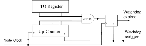
Figure 6: Implementation principle of watchdog timers.

As for the watchdog timer with random timeout $R_{3}$ in the resynchronization algorithm, the simplest implementation would load a uniformly distributed random value into the timeout register whenever the watchdog is re-triggered. Depending on the implementation technology, such random values can be generated either via true random sources (thermal noise) or pseudo-random sources (LFSRs) clocked by another ring oscillator. If we could guarantee that the content of the timeout and the random source can, by no means, read or probed somehow by anybody, such an implementation satisfies the model requirements. Alternatively, one could use random sampling per clock tick, which avoids storing the future timeout value and also converges to uniformly distributed timeouts for sufficiently large values of $R_{3}$.

Combined State Transition Conditions

Combining different state transition conditions (i)–(iii) via AND/OR requires some care, since an asynchronous state machine requires stable input signals in order not to become metastable during its state transition. Combining several conditions (i) does not cause any problems, since the memory flags ensure that all outputs are stable. Non-stable signals, like “$T_{1}$ AND $<n-f$ accept” require sampling via a flip-flop clocked by a stable signal. For example, the status of $<n-f=\neg\geq n-f$ is sampled when the signal reporting expiration of $T_{1}$ is issued. Similarly, it might happen that conditions requiring conflicting state transitions are satisfied at the same time, e.g., $(T_{2},\emph{accept})$ might expire simultaneously with the threshold of “$\geq f+1$ recover or accept” being reached.

Obviously, both of the above situations could create a metastable upset, either of the sampling flip-flop, or directly of the register(s) holding the node’s state. Fortunately, [theorem:stability]Theorem 4.4 revealed that this can happen during stabilization only. In regular operation, e.g. the critical threshold of $\geq n-f$ accept is always reached before $T_{1}$ expires. Thus, the former is acceptable, as metastable upsets occur rarely and increase convergence time only. Moreover, to further decrease the probability of a metastable upset that might affect stabilization time, it is perfectly feasible to insert a synchronizer or an elastic pipeline after the sampling flip-flop for capturing metastability [13]. This additional precaution merely increases the latency by a constant delay, which due to being restricted to the pulse synchronization component will not adversely affect the final precision and accuracy of the stabilized darts clocks.

7 Coupling of DARTS and Pulse Synchronization Algorithm

In this section, we describe how the self-stabilizing pulse synchronization protocol could be coupled with darts clocks. As this requires certain implementation details, we also sketch some ideas that might be used in a prototype implementation. The joint system provides a high-precision self-stabilizing Byzantine fault-tolerant clocking system for multi-synchronous GALS.

The coupling between the pulse synchronization protocol and darts clocks involves two directions:

1. The pulse synchronization protocol primarily monitors the operation of the darts clocks. As long as darts ticks are generated correctly, it must not interfere with the darts tick generation rules at all.

2. If darts clocks become inconsistent w.r.t. the behavior of the pulse synchronization protocol, the latter must interfere with the regular darts tick generation, possibly up to resetting darts clocks.

To assist the reader, we first provide a very brief overview of the original darts and its implementation.

7.1 DARTS Overview

darts clocks (called TG-Algs in the sequel) are instances of a simple synchronizer [35] for the $\Theta$-Model based on consistent broadcasting [31]. They generate ticks Tick (0), Tick (1), Tick (2), … approximately simultaneously at all correct nodes. Since actual darts ticks are just binary clock signal transitions, which cannot carry tick numbers, the original algorithm had to be modified significantly in order to be implementable in asynchronous digital logic. [fig:TGAlg]Figure 7 shows a schematic of a single TG-Alg for a 5-node system.

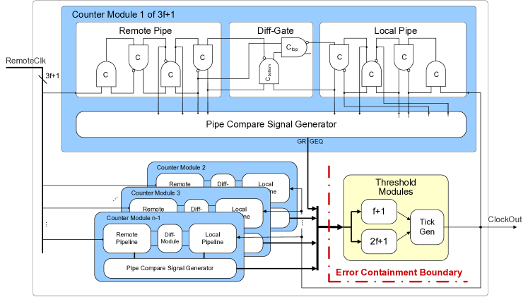
Figure 7: Schematic of darts TG-Alg Implementation

Key components of a TG-Alg are counter modules, one per remote TG-Alg, which just count the difference between the number of ticks generated locally and remotely. They are implemented using a pair of elastic pipelines [33], which implement FIFO buffers for signal transitions. Matching ticks in both pipelines, which are obviously irrelevant for the difference, are removed by the connecting Diff-Gate. The status ($>0$, $\geq 0$) of all counter modules is fed into two threshold modules, whose outputs trigger the generation of the next local tick. A detailed discussion of the implementation can be found in [10].

The correctness proof and performance analysis in [16, 17, 15] revealed that correct TG-Algs indeed generate synchronized clock ticks, in the presence of up to $f$ Byzantine faulty TG-Algs in a system with $n\geq 3f+2$ nodes: For any two correct nodes $p$, $q$, the number of clock ticks generated by $p$ and $q$ by time $t$ do not differ by more than a (very small) constant $\pi$, and the frequency of any correct clock (and thus the maximum drift $\rho$) is within a certain range. In addition, expressions (in the order of $\pi$) for the maximum size of the elastic pipelines in the counter modules were established, which guarantee overflow-free operation. Experiments with both FPGA and ASIC prototype implementations demonstrated that darts clocks indeed offer close to perfect synchronization and very reliable operation.

Nevertheless, as already mentioned, (almost) simultaneous start-up of all TG-Algs and at most $f$ failures during the whole life-time of the system are mandatory preconditions for these results to hold. darts neither supports late joining or recovery of TG-Algs, nor recovery from more than $f$ failures.

7.2 Required Extensions for Coupling DARTS and Pulse Synchronization

The major obstacle for supporting late joining of TG-Algs, removing spuriously generated ticks in the pipelines etc. are the anonymous clock ticks used in darts: Since they are just signal transitions on a single wire, they cannot encode any information except their occurrence time. The most important extension of darts is hence to add an additional bundled data wire to the clock signal, which carries 1 bit of data. This way, single ticks can be marked with a 1, distinguishing them from ordinary non-marked ticks that carry a 0.

We will actually mark every $T$-th darts tick, for some suitably chosen $T$. Such a marked tick $kT$, $k\geq 0$, is to be understood as the start of the $(k+1)$-st darts round, which consists of the marked darts tick $kT$ and $T-1$ subsequent unmarked ticks $kT+1,kT+2,\ldots,(k+1)T-1$; the marked tick $(k+1)T$ starts the next darts round. Note that the resulting darts ticks can be interpreted as a discrete, bounded clock operating modulo $T$. As darts rounds at any two correct TG-Algs are synchronous, marked ticks must always match in the pipelines of every counter, i.e., the Diff-Gate must always remove pairs of matching marked (or non-marked) ticks and can hence detect and remove any inconsistency.

The actual coupling between the instance of the pulse synchronization protocol and the darts clock running at node $i$ is accomplished by means of two signals, namely, $\mbox{\sc{darts}}_{i}$ and $\mbox{\sc{pulse}}_{i}$:

• $\mbox{\sc{darts}}_{i}$ reports darts rounds to the pulse synchronization protocol. The rising edge of the $\mbox{\sc{darts}}_{i}$ signal, which may trigger a switch from ready to propose; is issued when the darts clock of node $i$ generates tick $kT-X$, for some fixed $X<T$. The falling edge of $\mbox{\sc{darts}}_{i}$ reports the occurrence of the marked tick $kT$.

• $\mbox{\sc{pulse}}_{i}$ reports the generation of a pulse to the darts clock. Its rising edge is issued on the transition to accept, and its falling edge signals the expiration of a fixed timeout $T_{y}$ that is reset at the time the rising edge is transmitted.

The basic idea underlying the coupling of the pulse synchronization protocol and darts is to align marked ticks and pulses as follows: If the system operates normally, every correct node $i$ first reaches some darts tick $kT-X$ and issues $\mbox{\sc{darts}}_{i}=1$. Next, a pulse is generated at node $i$ by the the pulse synchronization protocol, which thus sets $\mbox{\sc{pulse}}_{i}=1$. Subsequently, the darts marked tick $kT$ occurs, which is signaled by $\mbox{\sc{darts}}_{i}=0$. Finally, the pulse timeout $T_{y}$ and hence $\mbox{\sc{pulse}}_{i}=0$ occurs. Normal operation thus expects that the darts marked tick (= the falling edge of $\mbox{\sc{darts}}_{i}$) occurs within the time window where $\mbox{\sc{pulse}}_{i}$ is 1. Provided that the timeout used for generating this window is chosen sufficiently large, namely, $\vartheta\rho(\pi+2d+1)$, this interleaving can indeed be guaranteed in normal operation.

As long as this is the case, we just let darts generate its ticks using its standard rules. Should a darts clock fail, however, such that $\mbox{\sc{pulse}}_{i}$ and $\mbox{\sc{darts}}_{i}$ are not properly interleaved, then we will force marking the next darts tick (and possibly resetting the TG-Alg, if needed) upon the falling edge of $\mbox{\sc{pulse}}_{i}$. darts ticks and pulses (as well as marked darts ticks at different nodes) will hence only be re-aligned in case of errors or desynchronization: As long as darts clocks work correctly, any two correct TG-Algs will mark tick $kT$ within the darts synchronization precision.

Provided that $X$ and $T_{y}$ are suitably chosen, it is not difficult to prove that the joint system consisting of pulse synchronization protocol and darts clocks will stabilize: After some unstable period, the pulse synchronization algorithm will stabilize, which we have proved to happen independently of the (non-)operation of darts clocks. When the pulse synchronization protocol eventually starts to generate synchronous pulses, the darts clocks will start to recover in a guided (synchronized) manner. When all correct darts clocks are eventually synchronized to within the intrinsic darts precision, the system will perpetually ensure the above interleaving at all correct nodes.

Some additional observations:

1. Since the darts precision is typically considerably smaller than the worst case pulse synchronization precision, the underlying darts clocks may be viewed as a “precision amplifier” (as well as a clock multiplier, see [sec:dartsextensions]Section 7.2).

2. There is no need to specify properties possibly achieved by darts clocks during their own recovery. We only require that they eventually reach full synchronization in the presence of synchronous pulses at all correct nodes. In practice, darts clocks will typically also gradually improve their synchronization precision during this interval.

3. Although the pulse synchronization algorithm stabilizes even when the darts clocks behave arbitrary, it is nevertheless the case that it achieves better pulse synchronization precision when the darts clocks are fully synchronized.

4. One might ask why we did not just use the $k$-th rising edge of $\mbox{\sc{pulse}}_{i}$ to mark the very next darts tick generated by the TG-Alg at node $i$. This simple solution has several major drawbacks. First, the pulse synchronization precision is typically worse than the synchronization precision provided by darts. Thus, every pulse would result in a temporary deterioration of the darts synchronization quality. Second, marked ticks are not necessarily generated exactly every $T$ darts ticks. And last but not least, since darts clocks and pulse synchronization execute completely asynchronously, marking darts ticks at pulse occurrence times would create the potential of metastability every $kT$ darts ticks, even if there is no failure at all.

7.3 DARTS $\Rightarrow$=¿ pulse synchronization

To implement this part of the coupling, every darts clock signals the upcoming occurrence of marked tick $kT$ to its local instance of the pulse synchronization protocol. This is accomplished by the rising edge of $\mbox{\sc{darts}}_{i}$, the dedicated darts signal, which is generated upon darts tick $KT-X$. If all correct nodes happen to do this within some time window when they are (w.r.t. the pulse algorithm) in state ready with $T_{3}<T_{4}$ already expired, all correct nodes will switch to state propose within $\pi$ time. Subsequently, they will all switch to state accept within $d$ time. To make sure that indeed all correct nodes are in state ready with $T_{3}$ already expired, up to small additional terms of $\mathcal{O}(d)$, we must choose the minimal duration of a darts round to be larger than $T_{2}+T_{3}+4d$, while $(T_{2}+T_{4})/\vartheta$ is to exceed its maximal duration. Assuming that $\rho<1.15$, [lemma:constraints]Lemma 3.4 shows that this is feasible up to $\vartheta\approx 1.064$, which is clearly within the reach of ring oscillators [32].

7.4 Pulse synchronization $\Rightarrow$=¿ DARTS

This part of the coupling between darts and the pulse synchronization protocol requires two mechanisms:

1. A way to force a marked darts tick at node $i$ upon the occurrence of the falling edge of $\mbox{\sc{pulse}}_{i}$, provided that no marked tick (i.e., the falling edge of $\mbox{\sc{darts}}_{i}$) has been generated while $\mbox{\sc{pulse}}_{i}$ was 1. This may also include recovering from a complete stall of the darts tick generation.

2. A way to recover accurate darts synchronization after forcing marked ticks, which may also include the need to get rid of any information from the preceding unstable period.

To achieve (1), we use a simple asynchronous circuit that supervises the interleaving of $\mbox{\sc{pulse}}_{i}$ and $\mbox{\sc{darts}}_{i}$, and generates a “force marking” signal if $\mbox{\sc{darts}}_{i}$ does not occur in time. Note that this device can be built in a way that entirely avoids metastability in case of normal operation. In an unstable period, however, it may happen that force marking occurs exactly at the time when darts generates its marked tick, so a metastable upset or two very close marked ticks (a forced and a regularly generated one) are possible.

There are several variants for implementing the forced marking itself, including the simplest variant of just resetting the TG-Alg in order to generate marked tick $0$. The need for possibly resetting a TG-Alg originates from the fact that stateful TG-Alg components may deadlock due to earlier failures. For example, a deadlocked pipe will never propagate ticks from its input to the Diff-Gate. Unfortunately, resetting TG-Algs complicates darts recovery considerably: If a TG-Alg reset would also reset the remote pipes of its counters, it might lose “fresh” marked ticks generated by remote TG-Algs. Hence, remote pipes should only be reset when the remote node is reset. However, since a remote node might never observe a discrepancy between darts rounds and pulses, this approach might end up in the pipe not being reset at all. This is problematic as it might effectively render the node faulty despite all its components being operational. Luckily, we may utilize the fact that solving (2) under the assumption that correct pipes are not deadlocked yields a trivial means to distinguish a locked pipe from an operational one: If the Diff-Gate cannot remove any ticks within a certain time interval after a (correct) pulse, the pipe must have deadlocked and can safely be reset. At the next pulse, all pipes will have recovered from previous deadlocks and a solution to (2) assuming deadlock-free pipes will succeed.

To explain how we achieve (2), we start with the observation that our way of marking every $T$-th tick implies that, for any two correct darts TG-Algs, it will always be a marked tick $kT$ from a remote node that is matched by the local marked tick $kT$ in every counter of [fig:TGAlg]Figure 7 when the Diff-Gate removes it. That is, if ever a marked tick is matching a non-marked tick in a counter, ticks have been lost or spuriously generated somewhere, or local and remote node are severely out of synchrony.

Assume for the moment that we could generate exactly one marked tick at every correct node, we made sure that no such tick is in the system before this happens, and that we have elastic pipelines of infinite size. The following simple strategy would eventually establish matching darts ticks: Whenever a Diff-Gate encounters a marked tick in one pipe matched by an ordinary tick in the other, it removes the ordinary tick only. At the pipe level, this rule implies that whatever the state of the pipes was before the marked ticks were generated, they will be cleared before the matching pair of marked ticks is removed. Since all darts tick generation rules ensure that no TG-Alg generates any tick $kT+1$, $kT+2$, … based on information from the previous darts round $k-1$ (consisting of darts ticks up to $kT-1$) all counter states will be valid as soon as the matching marked ticks $kT$ have been removed. As darts essentially generates ticks based on comparing the number of locally and remotely generated ticks, this is enough to ensure stabilization of the darts system; full darts precision will be achieved quickly because nodes “catch up”, i.e., generate tick numbers that at least $f+1$ correct darts clocks already reached, faster than “new ticks”, i.e., ones that no correct node generated yet, may occur.

The issue of finite-size pipes is (largely) solved by the pulse synchronization protocol: Pulses and hence marked ticks are generated close to each other, in a time window of at most $2d+T_{y}\in\mathcal{O}(d)$ (provided that $T_{y}$ is not unnecessarily large). Hence, apart from implementation issues, pipes that can accommodate all ticks that may be generated within this time window are sufficient for not losing any valid darts tick.

In reality, however, we cannot always expect the “single marked tick” setting described above: Elastic pipelines may initially be populated with arbitrarily many marked ticks from the unstable period. We must hence make sure that all these marked ticks (and the white ticks in between) are eventually removed, and that we do not generate new marked ticks close to each other. The pulse synchronization protocol will ensure that forced ticks are separated by $T$ darts ticks, and our implementations of (1) and (2) will ensure with a large probability that a forced marked tick will not be generated close to a marked tick generated regularly by darts. Under these conditions, it is a relatively easy task to clear all superfluous marked ticks between pulses.

For example, we could asynchronously reset the whole data flip-flop chain that holds the markings of the ticks (not the ticks themselves!) currently in a pipe shortly after the rising flank of $\mbox{\sc{pulse}}_{i}$. Enlarging $X$ and $T_{y}$ slightly, we can be sure that all TG-Algs will remove spurious markings from their pipes before any marked tick associated with the respective correct pulse is generated. Although this could generate metastability in the Diff-Gate, namely, when the tick at the head of the pipe is a marked tick and the Diff-Gate is about to act when the pipe is reset upon arrival of a new marked tick arrives, this cannot happen during normal operation.

References

- [1] M. Ben-Or, D. Dolev, and E. N. Hoch. Fast self-stabilizing byzantine tolerant digital clock synchronization. In Proc. 27th symposium on Principles of Distributed Computing (PODC), pages 385–394, 2008.
- [2] A. Berman and I. Keidar. Low-Overhead Error Detection for Networks-on-Chip. In The 27th International Conference on Computer Design (ICCD), 2009.
- [3] R. Bhamidipati, A. Zaidi, S. Makineni, K. Low, R. Chen, K.-Y. Liu, and J. Dalgrehn. Challenges and Methodologies for Implementing High-Performance Network Processors. Intel Technology Journal, 6(3):83–92, 2002.
- [4] D. M. Chapiro. Globally-Asynchronous Locally-Synchronous Systems. PhD thesis, Stanford University, 1984.
- [5] C. Constantinescu. Trends and Challenges in VLSI Circuit Reliability. IEEE Micro, 23(4):14–19, 2003.
- [6] A. Daliot and D. Dolev. Self-Stabilizing Byzantine Pulse Synchronization. CoRR, abs/cs/0608092, 2006.
- [7] A. Daliot, D. Dolev, and H. Parnas. Self-Stabilizing Pulse Synchronization Inspired by Biological Pacemaker Networks. In Proc. 6th Symposium on Self-Stabilizing Systems (SSS), 2003.
- [8] C. Dike and E. Burton. Miller and Noise Effects in a Synchronizing Flip-Flop. IEEE Journal of Solid-State Circuits, SC-34(6):849–855, 1999.
- [9] S. Dolev and J. L. Welch. Self-stabilizing clock synchronization in the presence of byzantine faults. Journal of the ACM, 51(5):780–799, 2004.
- [10] M. Ferringer, G. Fuchs, A. Steininger, and G. Kempf. VLSI Implementation of a Fault-Tolerant Distributed Clock Generation. IEEE Symposium on Defect and Fault-Tolerance in VLSI Systems (DFT), pages 563–571, 2006.
- [11] M. J. Fischer and N. A. Lynch. A Lower Bound for the Time to Assure Interactive Consistency. Information Processing Letters, 14:183–186, 1982.
- [12] E. G. Friedman. Clock Distribution Networks in Synchronous Digital Integrated Circuits. Proceedings of the IEEE, 89(5):665–692, 2001.
- [13] G. Fuchs, M. Függer, and A. Steininger. On the Threat of Metastability in an Asynchronous Fault-Tolerant Clock Generation Scheme. In Proc. 15th Symposium on Asynchronous Circuits and Systems (ASYNC), pages 127–136, Chapel Hill, N. Carolina, USA, 2009.
- [14] M. Függer. Analysis of On-Chip Fault-Tolerant Distributed Algorithms. PhD thesis, Technische Universität Wien, Institut für Technische Informatik, 2010.
- [15] M. Függer, A. Dielacher, and U. Schmid. How to Speed-Up Fault-Tolerant Clock Generation in VLSI Systems-on-Chip via Pipelining. In Proc. 8th European Dependable Computing Conference (EDCC), pages 230–239, 2010.
- [16] M. Függer and U. Schmid. Reconciling Fault-Tolerant Distributed Computing and Systems-on-Chip. Research Report 13/2010, Technische Universität Wien, Institut für Technische Informatik, 2010.
- [17] M. Függer, U. Schmid, G. Fuchs, and G. Kempf. Fault-Tolerant Distributed Clock Generation in VLSI Systems-on-Chip. In Proc. 6th European Dependable Computing Conference (EDCC), pages 87–96, 2006.
- [18] M. J. Gadlage, P. H. Eaton, J. M. Benedetto, M. Carts, V. Zhu, and T. L. Turflinger. Digital Device Error Rate Trends in Advanced CMOS Technologies. IEEE Transactions on Nuclear Science, 53(6):3466–3471, 2006.
- [19] E. Hoch, D. Dolev, and A. Daliot. Self-stabilizing Byzantine Digital Clock Synchronization. In Proc. 8th Symposium on Stabilization, Safety, and Security of Distributed Systems (SSS 2006), volume 4280, pages 350–362, 2006.
- [20] Internat. Technology Roadmap for Semiconductors, 2007.
- [21] D. J. Kinniment, A. Bystrov, and A. V. Yakovlev. Synchronization Circuit Performance. IEEE Journal of Solid-State Circuits, SC-37(2):202–209, 2002.
- [22] M. Malekpour. A Byzantine-Fault Tolerant Self-stabilizing Protocol for Distributed Clock Synchronization Systems. In Proc. 9th Conference on Stabilization, Safety, and Security of Distributed Systems (SSS), pages 411–427, 2006.
- [23] L. Marino. General Theory of Metastable Operation. IEEE Transactions on Computers, C-30(2):107–115, 1981.
- [24] C. Metra, S. Francescantonio, and T. Mak. Implications of Clock Distribution Faults and Issues with Screening them During Manufacturing Testing. IEEE Transactions on Computers, 53(5):531–546, 2004.
- [25] C. J. Myers. Asynchronous Circuit Design. John Wiley & Sons, Inc., 2001.
- [26] M. Pease, R. Shostak, and L. Lamport. Reaching Agreement in the Presence of Faults. Journal of the ACM, 27:228–234, 1980.
- [27] T. Polzer, T. Handl, and A. Steininger. A Metastability-Free Multi-synchronous Communication Scheme for SoCs. In Proc. 11th International Symposium on Stabilization, Safety, and Security of Distributed Systems (SSS 2009), pages 578–592, 2009.
- [28] C. L. Portmann and T. H. Y. Meng. Supply Noise and CMOS Synchronization Errors. IEEE Journal of Solid-State Circuits, SC-30(9):1015–1017, 1995.
- [29] P. J. Restle and others;. A Clock Distribution Network for Microprocessors. IEEE Journal of Solid-State Circuits, 36(5):792–799, 2001.
- [30] Y. Semiat and R. Ginosar. Timing Measurements of Synchronization Circuits. In Proc. 9th Symposium on Asynchronous Circuits and Systems (ASYNC), 2003.
- [31] T. K. Srikanth and S. Toueg. Optimal Clock Synchronization. Journal of the ACM, 34(3):626–645, 1987.
- [32] K. Sundaresan, P. Allen, and F. Ayazi. Process and temperature compensation in a 7-MHz CMOS clock oscillator. IEEE J. Solid-State Circuits, 41(2):433–442, 2006.
- [33] I. E. Sutherland. Micropipelines. Communications of the ACM, Turing Award, 32(6):720–738, 1989.
- [34] P. Teehan, M. Greenstreet, and G. Lemieux. A Survey and Taxonomy of GALS Design Styles. IEEE Design and Test of Computers, 24(5):418–428, 2007.
- [35] J. Widder and U. Schmid. The Theta-Model: Achieving Synchrony without Clocks. Distributed Computing, 22(1):29–47, 2009.