An Evolutionary Model for Collapsing Molecular Clouds and Their Star Formation Activity

Abstract

We present an idealized, semi-empirical model for the evolution of gravitationally contracting molecular clouds (MCs) and their star formation rate (SFR) and efficiency (SFE). The model assumes that the instantaneous SFR is given by the mass above a certain density threshold divided by its free-fall time. The instantaneous number of massive stars is computed assuming a Kroupa IMF. These stars feed back on the cloud through ionizing radiation, eroding it. The main controlling parameter of the evolution turns out to be the maximum cloud mass, $M_{\rm max}$. This allows us to compare various properties of the model clouds against their observational counterparts. A giant molecular cloud (GMC) model ($M_{\rm max}\sim 10^{5}~{}{\rm M}_{\odot}$) adheres very well to the evolutionary scenario recently inferred by Kawamura et al. (2009) for GMCs in the Large Magellanic Cloud. A model cloud with $M_{\rm max}\approx 2000~{}{\rm M}_{\odot}$ evolves in the Kennicutt-Schmidt diagram first passing through the locus of typical low- to-intermediate mass star-forming clouds, and then moving towards the locus of high-mass star-forming ones over the course of $\sim 10$ Myr. Also, the stellar age histograms for this cloud a few Myr before its destruction agree very well with those observed in the $\rho$-Oph stellar association, whose parent cloud has a similar mass, and imply that the SFR of the clouds increases with time. Our model thus agrees well with various observed properties of star-forming MCs, suggesting that the scenario of gravitationally collapsing MCs, with their SFR regulated by stellar feedback, is entirely feasible and in agreement with key observed properties of molecular clouds.

1 Introduction

A crucial ingredient in understanding the star formation efficiency (SFE) of giant molecular clouds (GMC) is the study of their evolution, from their formation to their destruction by the massive stars they form. A still unsolved problem is whether the GMCs are in approximate virial equilibrium, or rather they are in gravitational contraction. Initially, Goldreich & Kwan (1974) proposed that the supersonic linewidths observed in GMCs correspond to global gravitational contraction, but Zuckerman & Palmer (1974) readily argued that if all the molecular gas in the Galaxy were in free fall, then the total star formation rate (SFR) in the Galaxy would be about two orders of magnitude higher than observed (we will refer to this as the “SFR conundrum”). Zuckerman & Evans (1974) subsequently suggested that the linewidths could correspond to small-scale turbulent motions, giving rise to the notion that clouds are quasi-equilibrium entities, a notion that has survived until today (see e.g., the reviews by Mac Low & Klessen, 2004; McKee & Ostriker, 2007).

Since then, most theoretical models of star formation (SF) have been based on the assumption that turbulence provides support against the clouds’ self-gravity, and allows them to maintain a quasi-virial equilibrium state, thus preventing global collapse and maintaining a low global SFR (e.g., Norman & Silk, 1980; McKee, 1989; Matzner, 2002; Krumholz & McKee, 2005; Li & Nakamura, 2006; Nakamura & Li, 2007; Wang et al., 2010). In these models, the turbulence is maintained by the energy feedback into the cloud from the stars it forms. One interesting model where strict equilibrium was not assumed, was that by Krumholz et al. (2006), where the fully time-dependent Virial Theorem was solved numerically for a cloud under the influence of its self-gravity and the pressure produced by feedback from H II regions, although the cloud was restricted to have a spherical geometry, and mass loss by the cloud due to ionizing radiation by massive stars was not considered. Those authors found that clouds undergo a few expansion-contraction oscillations, until they are finally dispersed, and the SFEs over the clouds’ lifetimes were found to be $\sim 5$ – 10%. More recently, a similar model, with the same restrictions but including mass accretion from the environment, was considered by Goldbaum et al. (2011). In this model, the clouds again reach virial equilibrium, and maintain roughly constant column densities.

However, recent theoretical and observational evidence has suggested a return to the global gravitational contraction scenario of Goldreich & Kwan (1974) (e.g., Hartmann, Ballesteros-Paredes, & Bergin, 2001; Burkert & Hartmann, 2004; Hartmann & Burkert, 2007; Peretto, Hennebelle & André, 2007; Galván-Madrid et al., 2009; Vázquez-Semadeni et al., 2007, 2009; Csengeri et al., 2010; Schneider et al., 2010). Additionally, Clark & Bonnell (2005) have suggested that molecular cloud turbulence, rather than directly producing Jeans-unstable clumps, only produces the seed nonlinear density fluctuations for subsequent gravitational fragmentation, which proceeds on different timescales due to the spatial variations on the local free-fall time induced by the turbulence (Heitsch & Hartmann, 2008). But then, if we again allow for clouds and their substructures to be in gravitational contraction, it is necessary to find a solution for the SFR conundrum in this scenario. The semi-empirical model presented here investigates whether stellar feedback can accomplish this.

Our model is motivated by the numerical simulations of Vázquez-Semadeni et al. (2010), who have investigated the evolution of clouds formed by the collision of warm neutral medium (WNM) cylindrical streams, including stellar feedback from ionization heating from massive stars. Those authors found that the clouds are in general not stabilized by the feedback, but rather are either dispersed or continue to contract globally, depending on their mass. Here, we construct a model that attempts to capture the phenomenology observed in those simulations, scanning the space of the parameters that determine the physical properties of the cloud. Rosas-Guevara et al. (2010) have also presented a parameter-space study, but using numerical simulations, and without feedback, while Dib et al. (2011) have produced an analytical model similar to ours, but aimed at investigating the effect of varying metallicity on the SFE.

The plan of the paper is as follows. In section §2 we describe the general model, which we then calibrate against a fiducial numerical simulation from Vázquez-Semadeni et al. (2010) in §3. In §5 we compare the calibrated model against various observational properties of both large and small MCs, parameterized only by their mass. In §6 we present a discussion, and finally a summary and our conclusions in §7.

2 The Model

We construct a model for studying the SFE in a thin cylindrical cloud undergoing gravitational contraction, as observed in various simulations (Vázquez-Semadeni et al., 2007, 2010, 2011; Heitsch & Hartmann, 2008). The system is schematically illustrated in Fig. 1. In the simulations, the collision of warm neutral medium streams nonlinearly triggers thermal instability, forming a thin cloud of cold atomic gas (e.g., Hennebelle & Pérault, 1999; Koyama & Inutsuka, 2000, 2002; Walder & Folini, 2000), which becomes turbulent by the combined action of various dynamical instabilities (Hunter et al., 1986; Vishniac, 1994; Koyama & Inutsuka, 2002; Heitsch et al., 2005; Vázquez-Semadeni et al., 2006). The cloud soon begins to contract gravitationally as a whole. However, before this global collapse is completed, some local, nonlinear (i.e., large-amplitude) density enhancements produced by the initial turbulence manage to collapse on their own, since their local free-fall time is shorter than the average one for the entire cloud (Heitsch & Hartmann, 2008; Pon et al., 2011). These local collapses thus involve only a fraction of the cloud’s total mass. Also, we assume that the newly-formed stars feed energy back into the cloud. We only consider the ionizing radiation from massive stars, since this radiation is probably the dominant mechanism of stellar energy injection at the scale of GMCs (Matzner, 2002).

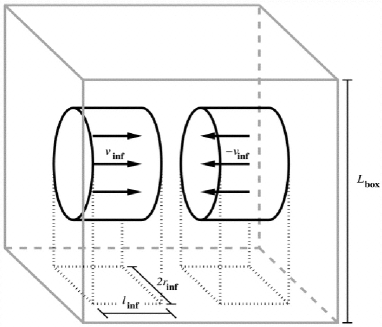
Figure 1: Model setup. Cylindrical streams of WNM are assumed to collide head-on to form first a flattened CNM cloud, which proceeds to collapse, becoming molecular and star-forming in the process. The main parameters of the model are the radius of the cylinders $R_{\rm inf}$, and the density and velocity of the inflowing warm gas.

In what follows, we investigate the competition between the cloud’s gravitational contraction and its destruction by the mass consumption by star formation (SF) as well as by the ionization produced by the newly formed massive stars. Below we describe how we calculate the contributions from these processes. It is important to note that we do not follow the chemistry, but rather consider that all the cold gas, either atomic or molecular, is involved in the gravitational contraction and, eventually, star formation.

2.1 Mass accretion

In our scenario, the cloud’s mass ($M_{\rm C}$) at time $t$ is given by

$$M_{\rm C}(t)=\int_{0}^{t}\dot{M}_{\rm inf}(t^{\prime})~{}{\rm d}t^{\prime}-M_{\rm S}(t)-M_{\rm I}(t),$$ (1)

where $\dot{M}_{\rm inf}(t)$ is the mass accretion rate onto the cloud from the WNM inflows, $M_{\rm S}(t)$ is the total mass in stars, and $M_{\rm I}(t)$ is the mass ionized by stellar feedback. Note that all these masses are considered to be functions of time. We assume that

$$\dot{M}_{\rm inf}(t)=2\,\rho_{\rm inf}\,v_{\rm inf}\,(\pi\,R_{\rm C}^{2}),$$ (2)

where $v_{\rm inf}$ is the inflow speed, $\rho_{\rm inf}=n_{\rm inf}\,\mu_{\rm H}\,{\rm m}_{\rm H}$ is the inflow mass density (with $n_{\inf}$ the number density of the inflows, $\mu_{\rm H}$ the mean atomic weight of the diffuse gas, and ${\rm m}_{\rm H}$ the atomic hydrogen mass). Note that $\pi\,R_{\rm C}^{2}$ is also the cross-sectional area of the thin, cylindrical, cold and dense cloud that forms by thermal instability at the layer compressed by the inflows. We take the cloud’s radius $R_{\rm C}(t)$ as being initially equal to the inflow radius $R_{\rm inf}$, and to later decrease as the cloud contracts gravitationally. The factor of 2 in eq. (2) represents the fact that there are two inflows, one on each side of the forming cloud.

2.2 Mass in Stars

We assume that the SFR is given by the ratio of the gas mass in the high-density tail ($n>n_{\rm SF}$) of the density distribution produced by the turbulence in the cloud, to its local free-fall time, $t_{\rm ff}(n_{\rm SF})=\sqrt{3\pi/32G\mu m_{\rm H}n_{\rm SF}}$. We refer to $n_{\rm SF}$ as the threshold density for star formation, and denote by $f(t)$ the fraction of the cloud’s mass that is at densities above $n_{\rm SF}$ (discussed in §2.6). We then have

$${\rm SFR}(t)=\frac{M_{\rm C}(t)}{t_{\rm ff}(n_{\rm SF})}\,f(t),$$ (3)

so that the mass in stars at time $t$ is

$$M_{\rm S}(t)=\int_{0}^{t}~{}{\rm SFR}(t^{\prime}){\rm d}t^{\prime}=\int_{0}^{t}~{}\frac{M_{\rm C}(t^{\prime})}{t_{\rm ff}(n_{\rm SF})}~{}f(t^{\prime})~{}{\rm d}t^{\prime}.$$ (4)

We assume that the initial density of the cloud is that of the cold neutral medium (CNM), in balance with the sum of the thermal and ram pressures of the inflows, as described in Vázquez-Semadeni et al. (2006). Typically, $n_{\rm CNM}\approx 100\,{\rm cm}^{-3}$, and we use a mean molecular weight of $\mu=2.35$, adequate for molecular gas. As the cloud evolves by contraction, the mean density evolves as determined by its mass and size, so that $\bar{\rho}=M_{\rm C}/\pi R_{\rm C}^{2}h$, where $h$ is the cloud thickness (cf. §2.4).

2.3 Ionized Mass

To model the cloud evaporation by massive stars, we use the results from Franco, Shore & Tenorio-Tagle (1994). These authors found that the cloud evaporation rate by a massive star near the cloud surface is

$$\dot{M}_{\rm I,sur}(t)\approx 2\pi R_{\rm S,0}^{2}m_{\rm H}\bar{n}c_{\rm s,I}\,\Big{(}1+\frac{5c_{\rm s,I}~{}t}{2R_{\rm S,0}}\Big{)}^{1/5},$$ (5)

where $t$ is the age of the massive star, $c_{\rm s,I}$ is the sound speed in the ionized gas, $\bar{n}=\bar{\rho}/\mu m_{\rm H}$ is the mean number density of the molecular cloud (MC), and $R_{\rm S,0}$ is the initial Strömgren radius of the massive star in the cloud ($R_{\rm S,0}=[3S_{*}/4\pi\alpha_{\rm B}(2\bar{n})^{2}]^{1/3}$, with $S_{*}$ a representative value of the UV Lyman-continuum photon flux (Franco, Shore & Tenorio-Tagle, 1994), and $\alpha_{\rm B}$ the recombination coefficient for the ionized gas). We assume that $R_{\rm S,0}$ is reached immediately at the instantaneous mean density of the cloud, which, in our model, is continually increasing as the cloud contracts. Therefore, over a short time interval $\Delta t$ (between $t$ and $t+\Delta t$), over which the cloud’s density can be assumed constant, a massive star near the cloud’s surface can ionize a mass $\Delta M_{\rm I,sur}=\dot{M}_{\rm I,sur}(t)\Delta t$.

In addition, we consider that, during the time interval $\Delta t$, the cloud forms $\Delta N_{\rm OB}(t)=x_{\rm OB}{\rm SFR}(t)\Delta t/\langle M_{\rm OB}\rangle$ new massive stars of average mass $\langle M_{\rm OB}\rangle$, where $x_{\rm OB}$ is the mass fraction of massive stars, which we calculate assuming an IMF from Kroupa (2001), with lower and upper mass limits of 0.01 and $60\,{\rm M}_{\odot}$ respectively. Defining a star as “massive” if it has a mass $M\geq 8{\rm M}_{\odot}$, we obtain $x_{\rm OB}=0.12$ and a mean massive-star mass $\langle M_{\rm OB}\rangle=17~{}{\rm M}_{\odot}$. Furthermore, in eq. (5) we take $S_{*}=2\times 10^{48}\,{\rm s}^{-1}$, $c_{\rm s,I}=12.8\,{\rm km}\,{\rm s}^{-1}$, and $\alpha_{\rm B}=2.6\times 10^{-13}\,{\rm cm}^{-3}\,{\rm s}^{-1}$ where we have assumed that the temperature of ionized gas in the HII region is $10^{4}\,{\rm K}$.

With the above considerations, and discretizing the time variable, the ionized mass at time $t_{i}$ is given by

$$M_{\rm I}(t_{i})=M_{\rm I}(t_{i-1})+\sum_{j=k}^{i}\Delta N_{\rm OB}(t_{j})\Delta M_{\rm I,sur}(t_{j}),$$ (6)

where $t_{k}$ is the time at which the oldest remaining OB stars were formed, $k=i-{\rm int}\left(t_{\rm OB}/\Delta t\right)$, ‘int’ is the integer function, and $t_{\rm OB}=5$ Myr is the main-sequence lifetime of our representative OB star. The second term in the right-hand side of eq. (6) thus gives the mass ionized over the time interval $\Delta t=t_{i}-t_{i-1}$ by the stars formed between $t_{k}$ and the present time, $t_{i}$. Note that we have neglected the possibility that part of the ionized gas can recombine and return to the cloud, as we expect the ionized gas to escape to the diffuse medium.

Finally, to account for the fact that the massive stars are born in dense environments, in eq. (5) we take the density as the maximum between the instantaneous cloud density $n(t)$ and $10^{3}{\rm~{}cm}^{-3}$ (typical of clumps), in order to avoid an over-ionization when the cloud density is low.

2.4 Global gravitational collapse.

Following the trend seen in the numerical simulations, we assume that our clouds evolve in two stages. First, a mass-growth stage occurs, during which the cloud (initially of zero mass) increases its mass by accretion from the WNM at constant radius and density, so that only its thickness increases (see, e.g., Vázquez-Semadeni et al., 2006, 2007; Folini & Walder, 2006), until it reaches its thermal Jeans mass. At that point, the second stage begins, during which the cloud undergoes global gravitational contraction. For circular modes in a self-gravitating isothermal sheet of finite thickness, the Jeans mass is given by (Larson, 1985):

$$M_{\rm J}=4.67\frac{c_{\rm s}^{4}}{G^{2}\Sigma}$$ (7)

where $c_{\rm s}$ is the cloud sound speed, and $\Sigma=M(t)/\pi R^{2}(t)$ is the surface density, with $M(t)$ and $R(t)$ being the instantaneous mass and radius of the cloud, respectively. In order to calculate the sound speed we first compute the cloud’s temperature. To do this, we use the fit by Koyama & Inutsuka (2002; see also the note in Vázquez-Semadeni et al. 2007) to the heating and cooling processes considered by Koyama & Inutsuka (2000). This allows us to solve for the temperature of thermal equilibrium (heating = cooling) as a function of the density. In this way, we get temperatures of $T\approx 42~{}{\rm K}$ for a density of $n=10^{2}~{}{\rm~{}cm}^{-3}$ and $T\approx 7~{}{\rm K}$ for $n\sim 10^{7}~{}{\rm~{}cm}^{-3}$.

During the mass-growth stage, over which the cloud’s radius remains constant ($R=R_{\rm inf}$), the cloud’s thickness $h$ is given by the condition of constant number density:

$$h(t)=\frac{M_{\rm C}(t)}{100\,\mu\,m_{\rm H}(\pi\,R_{\rm inf}^{2})}.$$ (8)

Once the collapse begins, we assume that the thickness remains constant at the final value achieved during the growth stage, and that its volume density increases only due to the radial contraction, as suggested by simulations including self-gravity (e.g., Vázquez-Semadeni et al., 2007, 2010, 2011; Heitsch & Hartmann, 2008). This assumption is equivalent to assuming that the average thickness of the cloud is much smaller than its Jeans length throughout its evolution. In general, this is a good approximation until when the cloud has contracted to radii of a few pc.

To determine the radial evolution during the contraction stage, we first calculate the acceleration at the cloud’s edge. We take a reference frame with its origin at the cloud’s center and with its $x$-axis along the inflow direction (i.e., perpendicular to the plane of our flattened cloud). We integrate over mass elements $\bar{\rho}~{}dzdydx$ located at a distance $[(R-z)^{2}+y^{2}+x^{2}]^{1/2}$ from the edge. At a certain time $t_{i}$, the acceleration at the cloud edge is

$$a(t_{i})=2\,G\,\bar{\rho}_{i}\,\int_{-R_{i}}^{R_{i}}\,dz\,\int_{0}^{\sqrt{R_{i}^{2}-z^{2}}}dy\,\int_{-h/2}^{h/2}\,\frac{R_{i}-z}{[(R_{i}-z)^{2}+y^{2}+x^{2}]^{3/2}}\,dx$$ (9)

where $\bar{\rho}_{i}=\bar{\rho}(t_{i})$ and $R_{i}=R_{\rm C}(t_{i})$. We solve the first integral analytically, while the second and third ones are solved numerically by the composite Simpson rule. After a small time increment $\Delta t=t_{i}-t_{i-1}$, the change in the cloud radius is:

$$R_{i+1}=R_{i}-v_{0,i}\,\Delta t-\frac{1}{2}a(R_{i})\Delta t^{2}$$ (10)

where the instantaneous velocity at time $t_{i}$ is $v_{0,i}=\sum_{j=0}^{i}a(R_{j})\Delta t$ for constant $\Delta t$.

Finally, we introduce a correction factor, representative of the fact that true gravitational collapse of a gaseous mass does not occur in strict free-fall, since thermal pressure is never completely negligible, as pointed out in the pioneering work by Larson (1969, Appendix C). There, he reported that the collapse of his simulations occurred in a time longer than the free-fall time by a factor of 1.58. Thus, at each timestep, we divide the radius given by eq. (10) by a factor $f_{\rm L}$, which we refer to as the “Larson parameter”, and calibrate in §3.

2.5 Density distribution

A key ingredient in our evolutionary model is the fraction of dense gas that is participating in the SF process, and therefore so is the evolution of the probability density function (PDF) of the cloud’s density field.

In our model, we consider that our clouds are born transonically turbulent, as a consequence of the various instabilities at play in the compressed layer between the streams (Vishniac, 1994; Walder & Folini, 2000; Heitsch et al., 2005, 2006; Vázquez-Semadeni et al., 2006). Also, in the absence of direct stellar irradiation, the temperature in the cold gas varies at most by factors of a few for densities $100<n<10^{7}{\rm~{}cm}^{-3}$, and thus, as a first approximation, we consider it to be isothermal. Therefore, we assume that the density field within the cloud is initially characterized by a lognormal PDF, appropriate for supersonically turbulent, isothermal gas (Passot & Vázquez-Semadeni, 1998). The PDF is then given by

$$P(s)=\frac{1}{\sqrt{2\pi\sigma_{s}^{2}}}~{}{\rm exp}\left[-\frac{(s-s_{\rm p})^{2}}{2\sigma_{s}^{2}}\right],$$ (11)

where

$$s\equiv\ln(\rho/\bar{\rho}),~{}~{}~{}s_{\rm p}=\ln(\rho_{\rm p}/\bar{\rho})=-\sigma_{s}^{2}/2,$$ (12)

with $\rho_{\rm p}$ the peak density, and

$$\sigma_{s}^{2}=\ln(1+b^{2}\mathcal{M}_{\rm rms}^{2}),$$ (13)

where $b$ is a proportionality constant related with the compressibility induced by the turbulent forcing, which for simplicity we take equal to unity (see e.g., Vázquez-Semadeni, 1994; Padoan et al., 1997; Passot & Vázquez-Semadeni, 1998; Federrath, Klessen & Schmidt, 2008).

However, more recent numerical and observational studies suggest that the density PDF in gravitationally contracting systems does not preserve its lognormal shape during the collapse, but rather develops a power-law tail at high densities (Klessen, 2000; Dib & Burkert, 2005; Vázquez-Semadeni et al., 2008; Kainulainen et al., 2009; Kritsuk et al., 2011; Ballesteros-Paredes et al., 2011b). In particular, Kritsuk et al. (2011) have suggested that the final slope should be in the range [3/2,7/4], but at the present time we know of no theoretical prediction as to how the slope nor the transition point between the lognormal and the power law should evolve in time. We experimented with various options for modeling the evolution of the PDF’s power-law tail, but found the behavior to be very sensitive to the parameters used, while we had no physical ways of constraining them. Finally, Kritsuk et al. (2011) proposed that the origin of the power-law tail is the development of local collapsing flows, that may have either Larson-Penston (Larson, 1969; Penston, 1969) or Shu (1977) density profiles. In this case, the power-law tail is an effect of the gravitational collapse rather than its cause, and thus it should not be counted as providing turbulent seeds for future collapses. For all of these reasons, we do not consider the power-law form of the PDF, and stick to the lognormal.

It is worth noting that the density PDF we consider here refers only to the cold (approximately isothermal) gas that makes up the cloud, and not to the entire gas contents of the system. This means that this PDF is not directly comparable to that observed in the numerical simulations of the same process, which corresponds to thermally-bistable gas. Thus, we did not consider the possibility of using a PDF extracted from numerical simulations, either.

We model the evolution of the lognormal density PDF as follows. First, as indicated by eq. (12), the mean of the PDF is given by the cloud’s mean density, given by $\bar{\rho}=M_{\rm C}/\pi R_{\rm C}^{2}h$. In turn, we prescribe that $\bar{\rho}$ varies as follows. During the mass-growth stage, it remains constant, at $100{\rm~{}cm}^{-3}$. Once the contraction stage begins, it increases, causing the density PDF to shift to higher values. Eventually, however, the SFR becomes large enough that the ionization by newly born massive stars reduces the cloud’s mass rapidly enough as to cause the PDF to shift back towards lower densities again.

Second, the standard deviation of the PDF is determined by the turbulent rms Mach number, as indicated by eq. (13). Unfortunately, the evolution of the turbulent component of the Mach number remains rather uncertain. Standard relations, such as Larson’s (1981) velocity dispersion size cannot be assumed here. Indeed, in our collapsing-cloud scenario, the majority of the velocity dispersion is due to the contracting motions (Ballesteros-Paredes et al., 2011) rather than to random turbulent motions, and should not be counted as turbulence capable of producing new density fluctuations suceptible of subsequent collapse.

Of course, it is natural to assume that a fraction of the kinetic energy in the collapsing motions will be transferred to random motions, but this problem remains largely unexplored in the case of gaseous media. Vázquez-Semadeni et al. (1998) numerically investigated the scaling of the non-collapsing component of the velocity dispersion in collapsing spherical clouds. Those authors found that the turbulent velocity dispersion scaled as $\rho^{x}$, with $x\in[1/4,1/2]$, depending on the particular setup of the collapse and on the presence of magnetic fields. However, that study was performed at low resolution and was restricted to spherical geometry, so it cannot be taken as definitive. More recently, Klessen & Hennebelle (2010) suggested that the rate of kinetic energy injection by the warm neutral streams feeding a molecular cloud is at least one order of magnitude larger than the rate of turbulent energy dissipation within the clouds. However, these estimates are not enough to properly constrain the evolution of the turbulent kinetic energy in our model clouds. Thus, we simply take a constant value of the turbulent Mach number, which represents a compromise between turbulent decay by dissipation and feeding of the turbulence by transfer from the collapsing motions. This thus implies that the width of the PDF in our model remains constant through the cloud’s evolution as well. We take this constant value of the turbulent Mach number as $\mathcal{M}_{\rm rms}=3$, the canonical value for the cold neutral medium (Heiles & Troland, 2003).

2.6 Star-forming mass fraction

Finally, as mentioned in §2.2, we assume that only gas with number density higher than a threshold value $n_{\rm SF}$ participates in the instantaneous SF process. This amounts to assuming that $n_{\rm SF}$ is sufficiently larger than the cloud’s mean density $\bar{n}$ as to guarantee that ${t_{\rm ff}}(n_{\rm SF})\ll{t_{\rm ff}}(\bar{n})$, where ${t_{\rm ff}}(n)$ is the free-fall time corresponding to density $n$. In a sense, this prescription may be thought of as the model’s analogue of sink particles in a numerical simulation (Bate et al., 1995; Federrath et al., 2010), in which gas at sufficiently high densities is replaced by point mass particles representing collapsed objects.

Thus, for the assumed lognormal PDF the fraction of dense gas that forms stars is given by

$$f(t)=\frac{1}{2}\left[1-{\rm erf}\left(\frac{2\,s_{\rm SF}(t)-\sigma_{s}^{2}}{\sqrt{2}\sigma_{s}}\right)\right],$$ (14)

where $s_{\rm SF}={\rm ln}(\rho_{\rm SF}/\bar{\rho})$, and $\rho_{\rm SF}$ is the volume density corresponding to $n_{\rm SF}$ (see also Elmegreen, 2002; Krumholz & McKee, 2005; Dib et al., 2011). The value of $n_{\rm SF}$ is calibrated against a numerical simulation by Vázquez-Semadeni et al. (2010) in §3.

2.7 Temporal evolution

With all the above ingredients, we discretize eq. (1) as

$$M_{\rm C}(t_{i})=\sum_{j=0}^{i}\dot{M}_{\rm inf}(t_{j})\Delta t-\sum_{j=0}^{i}\frac{M_{\rm C}(t_{j})\,\Delta t}{t_{\rm ff}(t_{j})}\,f(t_{j})-\Big{[}M_{\rm I}(t_{i-1})+\sum_{j=k}^{i}\Delta N_{\rm OB}(t_{j})\Delta M_{\rm I,sur}(t_{j})\Big{]}$$ (15)

We integrate this equation numerically over time, taking $\Delta t=4\times 10^{-4}\,{\rm Myr}$. We choose this value as a reasonable compromise between speed and accuracy, after experimenting with timesteps down to 0.01 times this value, from which we found (with arbitrary free parameters) that the chosen value gives already well-converged values of the final cloud masses, the variable that turned out to be most sensitive to the size of the timesteps.

We consider that the cloud’s evolution ends either because the cloud gets completely evaporated by the massive-star ionization or because its average density reaches $n_{\rm SF}$, a point at which the remaining mass is fully converted into stars and the cloud disappears.

3 Calibration of the model

With all the model ingredients defined, we now proceed to calibrate it by matching it to one of the numerical simulations by Vázquez-Semadeni et al. (2010). We consider the simulation labeled SAF1 in that paper, which most resembles the physical conditions built into our model. The label SAF indicated that it contained small-amplitude initial velocity fluctuations ($\sim 2$% of $v_{\rm inf}$), which were sufficient to trigger the instabilities responsible for turbulence production in the forming cloud, but not large enough to significantly distort its sheet-like geometry.

The simulation considered the collision of two cylindrical WNM streams with $n_{\rm inf}=1\,{\rm cm}^{-3}$, $T_{\rm inf}=5000\,{\rm K}$, inflow radius of $R_{\rm inf}=64\,{\rm pc}$, and an initial inflow speed $v_{\rm inf}=7.5{\rm~{}km~{}s}^{-1}$. Thus, for our calibration purposes, we use these same values for our model, except for $v_{\rm inf}$. We do this because, in the simulation, the inflow speed decreases over time, because the rear end of the inflowing cylinder leaves a vacuum behind it. As a consequence, in the reference frame of the inflow, the inflow’s rear end tends to re-expand into this vacuum, producing a velocity gradient along the cylinder. Instead, in the model we use a constant inflow speed, and thus we take a smaller value, representative of the time-averaged speed in the simulation. We find that a value of $v_{\rm inf}=4.5{\rm~{}km~{}s}^{-1}$ provides the best match for the evolution of the simulation cloud’s mass. Also, we find that the temporal evolution of the cloud’s radius is best matched with a value of the Larson parameter of $f_{\rm L}=1.7$, very close to the original value of 1.58 originally proposed by Larson (1969). We show the evolution of these quantities for both the simulation and the model in Fig. 2. Note that the evolution for the model with the ionizing stellar feedback turned both on and off is shown. We refer to the model with feedback off as the LN-F0 case, and to the one with the feedback on, as the LN-F1 case.

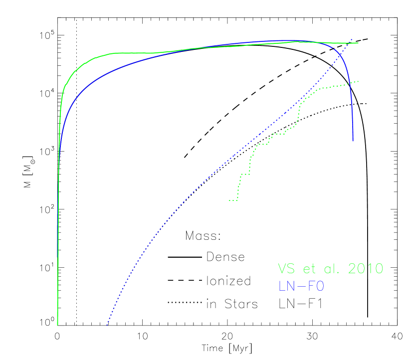
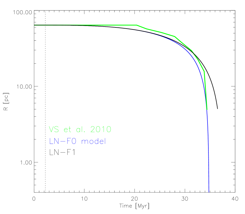
Figure 2: Left: Evolution of the dense gas mass, ionized gas mass, and mass in stars for the model cloud with parameters that best match the corresponding quantities (except for the ionized mass, which is not measured) in the SAF1 simulation of Vázquez-Semadeni et al. (2010). The green lines represent the simulation, the blue lines represent the model cloud with stellar feedback turned off, and the black lines represent the model cloud with the stellar feedback turned on, with $n_{\rm SF}=10^{6}{\rm~{}cm}^{-3}$. The vertical line represents the beginning of global collapse. Right: Evolution of the cloud radius in the model and in the simulation, with the same color coding as in the left panel.

Next, keeping the above parameters fixed, we vary the $n_{\rm SF}$ parameter, the density threshold for star formation, to match the SFR and SFE of the simulation, with the SFE being defined as

$${\rm SFE(t)}=\frac{M_{\rm S}(t)}{M_{\rm C}(t)+M_{\rm S}(t)+M_{\rm I}(t)},$$ (16)

where $M_{\rm C}$ is the dense gas mass, $M_{\rm S}$ is the total mass in stars, $M_{\rm I}$ is the total mass ionized by stars, all quantities being time-dependent. Figure 3 shows the evolution of the SFR and SFE of the model for $n_{\rm SF}=10^{5}$, $10^{6}$, and $10^{7}{\rm~{}cm}^{-3}$, and compares them with the evolution of the corresponding quantities in the simulation, showing that the best match is obtained with a value $n_{\rm SF}=10^{6}{\rm~{}cm}^{-3}$, which we use in the rest of the paper. This value is reassuring since, on the one hand, it is comparable to the sink-formation density threshold used in the numerical simulations (Vázquez-Semadeni et al., 2007, 2010), and on the other, it is high enough that the material above those densities can be safely assumed to be locally gravitationally bound (Galván-Madrid et al., 2007; Heitsch & Hartmann, 2008).

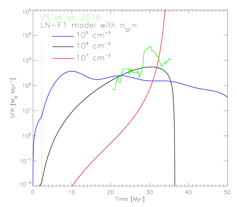
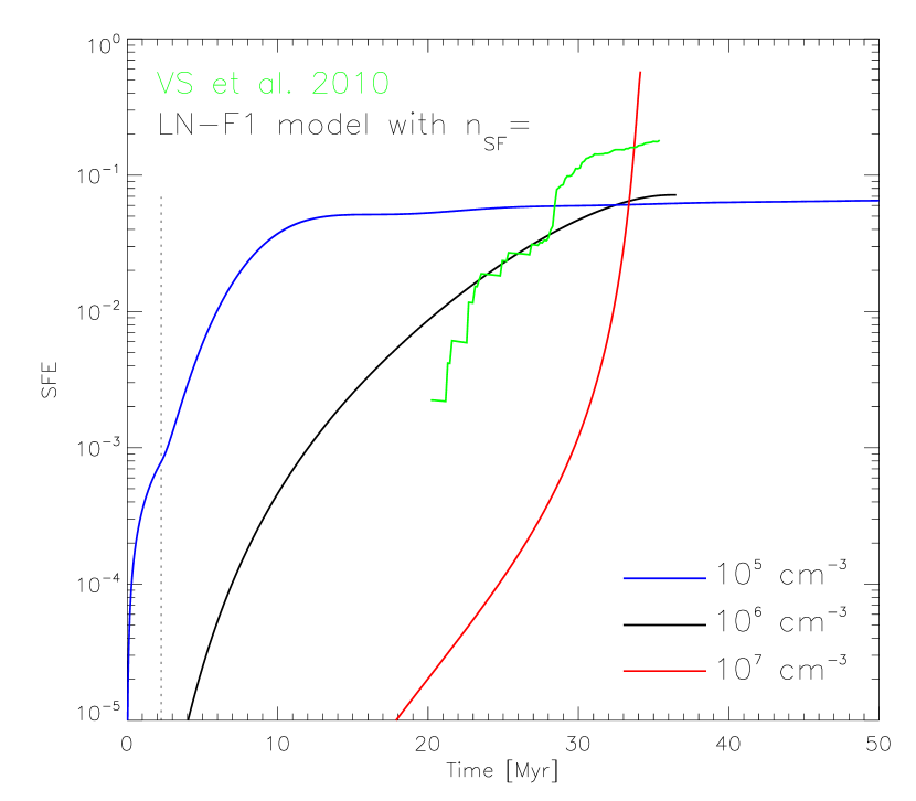
Figure 3: Left: Evolution of the star formation rate (SFR) for the model cloud for the cases $n_{\rm SF}=10^{5}$, $10^{6}$, and $10^{7}{\rm~{}cm}^{-3}$, compared to the evolution of the SFR in the SAF1 simulation of Vázquez-Semadeni et al. (2010). Right: Same as the left panel, but for the star formation efficiency (SFE). The green lines represent the numerical simulation.

4 Discussion of the calibrated model’s evolution

Once the model parameters have been calibrated with the SAF1 simulation, it is illustrative to discuss the general features of the model cloud’s evolution, which hold qualitatively for the other cases we explore in §5, where varying only the inflow radius $R_{\rm inf}$ we are able to match and explain several observed features of molecular clouds and their star-forming activity.

First, we note from the right panel of Fig. 2 that the radius of the model with feedback (LN-F1) evolves slightly more slowly than that of the case without feedback (LN-F0). This is because the stellar feedback erodes the cloud through ionization, thus reducing its mass, which in turns causes a lower gravitational acceleration, thus slowing the collapse. We also note that the radius of the LN-F0 case approaches zero at late times, while that of the LN-F1 ends at a finite radius, implying that the evolution is terminated because the cloud is completely evaporated before it reaches zero radius (see below).

Second, from the left panel of Fig. 2, we note that the dense gas mass of both the LN-F0 and LN-F1 models decreases at late times. This is because even in the non-feedback LN-F0 model, gas is consumed due to the conversion of gas to stars. However, we see that the mass consumption is much more abrupt in the LN-F0 model, while in the LN-F1 model it proceeds more slowly. This indicates that the feedback inhibits star formation to the level that the mass consumed by ionization from the feedback is less than the mass that would be consumed by star formation were there no feedback. Nevertheless, note that the dense gas mass in the LN-F1 model approaches zero at the end of the evolution, indicating that all of the cloud’s mass is used up by the combined action of ionization and star formation. This corresponds to the well known fact that clusters eventually destroy their natal cloud, and are left with no gas around them after several million years (Leisawitz et al., 1989).

Finally, note from Fig. 4 that both the SFR and the SFE increase at an ever faster pace until the end of the simulation in the non-feedback case LN-F0, while their growth slows down in the case of LN-F1. In this case, the SFR eventually begins to decrease and goes to zero at the end of the evolution, as the dense gas mass is completely consumed by the ionization, leaving no further fuel for star formation. Instead, the SFR in the LN-F0 case would reach a singularity at a finite time were it not for the time discretization of our model.

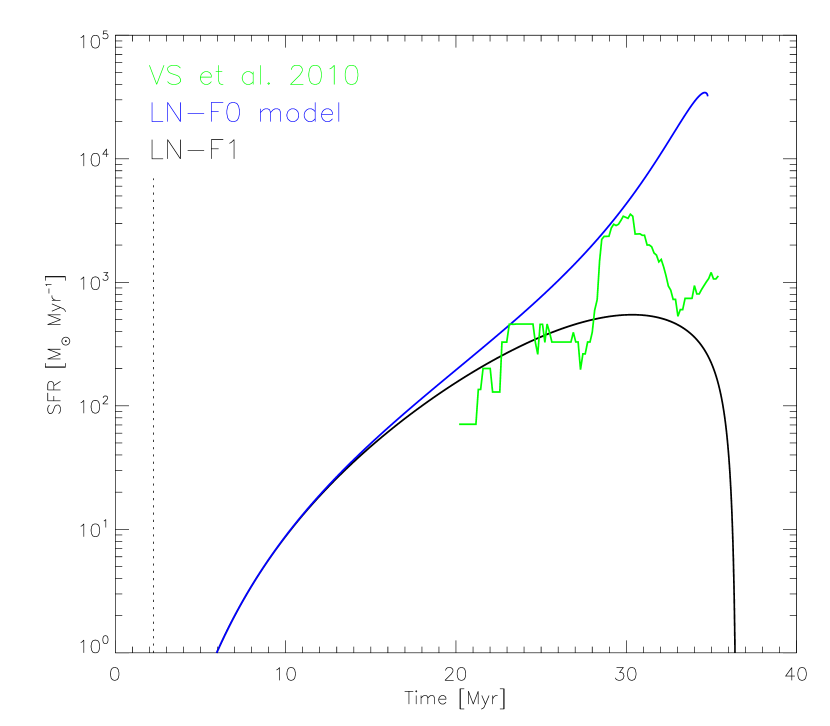
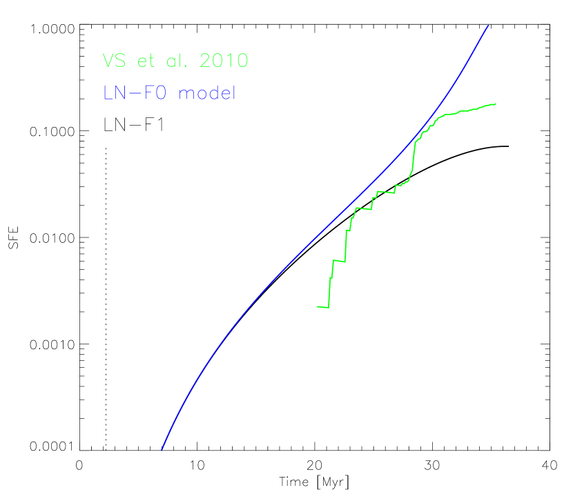
Figure 4: Evolution of the SFR (left) and the SFE (right) of the calibrated model with $n_{\rm SF}=10^{6}{\rm~{}cm}^{-3}$ for a case with feedback turned off (LN-F0, blue line) and a case with feedback on (LN-F1, black line). The green lines represent the numerical simulation. The LN-F0 model has accelerating SFR and SFE, while they decelerate for model LN-F1. See also discussion in §6.3

5 Comparison with observations and previous work

We now proceed to compare the results of our model with related observational results. For the various comparisons, we vary only the inflow radius parameter, $R_{\rm inf}$, which determines the maximum dense gas mass attained by the model.

5.1 Evolutionary stages

As a first case in point, we consider the evolutionary stages of the clouds. Recently, Kawamura et al. (2009) have suggested that GMCs in the Large Magellanic Cloud undergo four evolutionary stages. In the first stage (Type I, with a duration of $\sim 7$ Myr and a median mass $M_{\rm tI}\sim 10^{4.8}~{}{\rm M}_{\odot}$), the GMCs show no sign of massive star formation. In the second stage (Type II; 14 Myr; $M_{\rm tII}\sim 10^{5.2}~{}{\rm M}_{\odot}$), the GMCs have only HII regions, while in the third (Type III; 6 Myr; $M_{\rm tIII}\sim 10^{5.4}~{}{\rm M}_{\odot}$ ), the GMCs contain both HII regions and clusters. Finally, the last stage (IV) corresponds to the time when the GMCs have been completely dispersed, and only young clusters and/or SNRs are found.

Because the masses of the clouds in their sample are near $10^{5}{\rm M}_{\odot}$, we choose an inflow radius $R_{\rm inf}=100$ pc, which gives a maximum cloud mass ($M_{\rm max}$) of slightly over $10^{5}~{}{\rm M}_{\odot}$, thus making it directly comparable to their cloud sample. Figure 5 shows the evolution of both the number of massive stars in the model cloud (top panel) and the masses of the dense gas, ionized gas, and stellar components of the cloud (bottom panel). For comparison with the cloud types defined by Kawamura et al. (2009), here we define Type I as the epoch when the model cloud has less than one massive star, Type II as the period when the cloud has less than 20 massive stars, and Type III as the period when the cloud has more than 20 massive stars. We see that the model cloud spends $\sim 5$ Myr as a Type I, $\sim 12$ Myr as a Type II, and $\sim 10$ Myr as a Type III, noting that after such a time the cloud’s mass has decreased by more than a factor of 2, and may be considered to be on its way to disappearing.

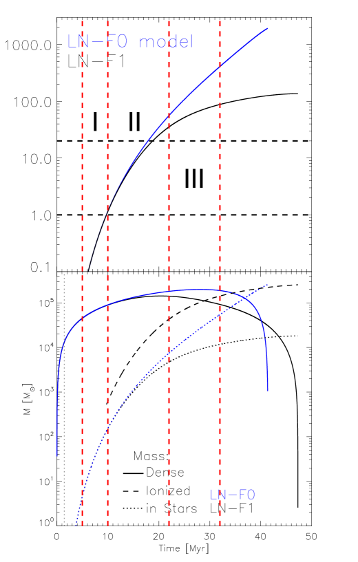
Figure 5: Top: Evolution of the number of massive stars in the model cloud with $R_{\rm inf}=100$ pc, showing the periods which roughly correspond to the cloud types defined by Kawamura et al. (2009). Bottom: Evolution of the dense gas, ionized and stellar masses for this cloud.

We also note from the bottom panel of Fig. 5, that the dense gas mass of the model cloud varies only moderately during the time it spends as an either Type I, II or III cloud, although a net increase from Type I to Type II is apparent. Moreover, because the cloud’s mass decreases by over a factor of 2 while it is in the Type III stage, a significant scatter in cloud masses is expected in this class, as is indeed observed in Fig. 12 of Kawamura et al. (2009).

From the above discussion, we thus conclude that the evolution of our model GMC, with $R_{\rm inf}=100$ pc, compares well, both qualitatively and quantitatively, with the evolutionary scheme proposed by Kawamura et al. (2009) for GMCs in the LMC.

5.2 Fiducial model vs. OMC-1

Next, we compare our model cloud with the physical conditions of real star-forming regions. As an example, we choose the clump known as OMC-1 in the Orion Molecular Cloud, which can be considered a typical massive star-forming region, and has been extensively studied. The total gas mass in OMC-1 is $\sim 2200\,{\rm M}_{\odot}$ (Bally et al., 1987), the size is $\sim 1.35\,{\rm pc}$ (which implies a number density $\sim 1.54\times 10^{4}\,{\rm cm}^{-3}$), and the mass in stars is $\sim 500\,{\rm M}_{\odot}$, which implies that the average SFR is $\langle{\rm SFR}\rangle\gtrsim 2.5\times 10^{-4}\,{\rm M}_{\odot}{\rm yr}^{-1}$, assuming a stellar age spread of $\lesssim 2\,{\rm Myr}$ (see Vázquez-Semadeni et al., 2009, and references therein).

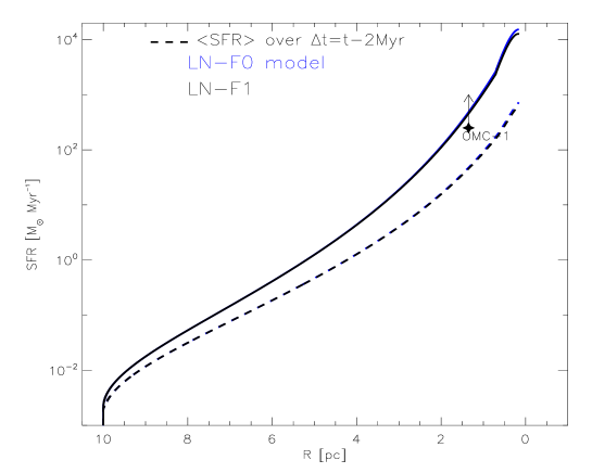
Figure 6: Evolution of a model cloud with $R_{\rm inf}=10$ pc in a SFR vs. size ($R$) diagram. Note that the size axis is reversed, so that the cloud evolves from left to right as it contracts gravitationally. Also plotted is the locus of the OMC-1 star-forming region in this diagram, showing that the model comes very close to that locus towards the end of its evolution.

To compare with this, we choose a value of $R_{\rm inf}=10$ pc for our model, which at $t=27.6$ Myr has the same density as OMC-1, making it directly comparable to the latter. At this time, the model cloud has a mass $M\approx 1800~{}{\rm M}_{\odot}$, a mass in stars $\approx 200\,{\rm M}_{\odot}$, and size (diameter) $\approx 1.9$ pc. Moreover, the average SFR over the last 2 Myr (the age dispersion used to compute the SFR of OMC-1) is $\langle{\rm SFR}\rangle\approx 100~{}{\rm M}_{\odot}~{}{\rm Myr}^{-1}$ (see Figure 6). These values are in very good agreement with the estimates for OMC-1, suggesting that our evolutionary model correctly describes this cloud.

5.3 Kennicutt-Schmidt relation.

Another possible point of comparison of our model with observational data is provided by the so-called Kennicutt-Schmidt relation. Ever since the seminal paper by Schmidt (1959), it has been well known that there exists a relationship between the SFR and the gas density in galaxies. Four decades later, collecting data from various surveys of nearby normal and starburst galaxies, Kennicutt (1998b) found a clear correlation between the galaxy-averaged SFR surface density ($\Sigma_{\rm SFR}$) and the galaxy-averaged total gas surface density ($\Sigma_{\rm gas}=\Sigma_{\rm HI}+\Sigma_{\rm H_{2}}$, where $\Sigma_{\rm HI}$ and $\Sigma_{{\rm H}_{2}}$ are the HI and H₂ surface densities, respectively) of the form $\Sigma_{\rm SFR}\propto\Sigma_{\rm gas}^{N}$, with $N\approx 1.4$.

Recent observations of external galaxies with high spatial resolution (on scales of fractions of kpc) show that $\Sigma_{\rm SFR}$ scales almost linearly with $\Sigma_{\rm H_{2}}$, while no clear correlation exists with $\Sigma_{\rm HI}$ (see e.g., Wu et al., 2005; Bigiel et al., 2008). However, observations of individual clouds (e.g., Evans et al., 2009; Heiderman et al., 2010) systematically show larger values of $\Sigma_{\rm SFR}$ than those implied by the fits by Kennicutt (1998b), Bigiel et al. (2008), and Wu et al. (2005). Moreover, the SFRs derived by Heiderman et al. (2010) for their massive clump sample were obtained using extragalactic methods (taken from Wu et al., 2010), and they warn that this could cause the SFRs they report to be underestimated by up to 0.5–1 orders of magnitude, implying an even stronger disagreement with the galaxy-scale measurements.

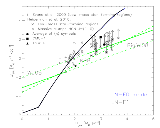
Figure 7: SFR surface density $\Sigma_{\rm SFR}$ vs. gas surface density $\Sigma_{\rm gas}$. The dashed line represents the Kennicutt-Schmidt relation, while the lower dotted line represents the observational fit by Bigiel et al. (2008) and the top dotted line is the fit by Wu et al. (2005). We also plot the data for individual low- to intermediate-mass star-forming regions by Evans et al. (2009) (+ symbols) and Heiderman et al. (2010) ($\times$ symbols) and for massive clumps by Heiderman et al. (2010) ($\ast$ symbols). The filled square represents OMC-1 (see Vázquez-Semadeni et al., 2009) and the filled triangle is Taurus (see, e.g., Heiderman et al., 2010). The arrows in the massive clumps from the latter authors indicate the likely correction to the SFR due to their application of extragalactic methods to Galactic regions. The solid black line shows the evolution of our calibrated model with $R_{\rm inf}=10$ pc.

These cloud-scale observations occupy a well-defined locus in $\Sigma_{\rm gas}-\Sigma_{\rm SFR}$ space, which can be compared with our model. For this task, we choose an inflow radius $R_{\rm inf}=10$ pc, for which our model reaches a maximum mass of $M_{\rm max}\approx 2000~{}{\rm M}_{\odot}$, almost identical to the median mass of the Evans et al. (2009) sample. In Fig. 7 we then plot the evolution of this model, as well as the loci of the clouds from the Evans et al. (2009) and Heiderman et al. (2010), adding an upwards-pointing arrow to the latter points, of length corresponding to one order of magnitude, to indicate the likely underestimation of the SFR for massive clumps by the latter authors. We also plot the data from OMC-1 (from Vázquez-Semadeni et al., 2009) and Taurus (see e.g., Heiderman et al., 2010). The model evolves from low to high values of both $\Sigma_{\rm gas}$ and $\Sigma_{\rm SFR}$.

It is interesting to note that the model passes first through the locus of the low-mass star-forming clouds and later near the locus of the clumps forming massive stars. This means that the model predicts that present-day, relatively quiescent, low-mass-star forming clouds may evolve into massive-star-forming ones in a few to several Myr. A similar conclusion was reached through numerical simulations by Vázquez-Semadeni et al. (2009). This reinforces the idea that the dispersion of the observational data is due to different evolutionary states of the clouds in a sample (see, e.g., Bigiel et al., 2010).

5.4 Stellar age distribution

One important prediction of our model is that the SFR increases over time. This is because, as the cloud contracts and its mean density increases, the fraction of star-forming gas in the cloud increases. An increasing SFR has already been proposed by Palla & Stahler (1999, 2000, 2002) on the basis of the age distribution in various low- and high-mass clusters. However, this result has been questioned, since there is evidence suggesting that the older stars are not genuine members of the clusters, but rather belong to a different population (Hartmann, 2003; Ballesteros-Paredes & Hartmann, 2007; Heitsch & Hartmann, 2008). Moreover, Hartmann (2003) has posed the conundrum that, if most clouds form at an accelerated pace only over the last few Myr, and form stars at a very slow rate over the previous 10 Myr or so, most clouds should be found to be in the slow-star-forming period, but this is not what is observed. Our evolutionary scenario for clouds may offer a solution to this debate.

Because in our model we compute the total mass of stars ($\Delta M$) formed at each time step, we can readily obtain the total number of stars formed during that time step as the integral over all masses of the IMF, normalized to $\Delta M$. The left panel of Fig. 8 shows the stellar age histogram for our calibrated model, with $R_{\rm inf}=10$ pc ($M_{\rm max}\approx 2000{\rm M}_{\odot}$) at the end of its life – i.e., when it has completely lost its gas. We show the histograms for a case with feedback off (model LN-F0) and one with feedback on (model LN-F1). It is clear from this figure that indeed the age distribution is concentrated towards young ages, although a few older stars exist.

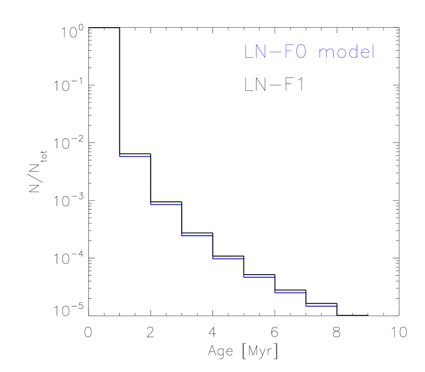
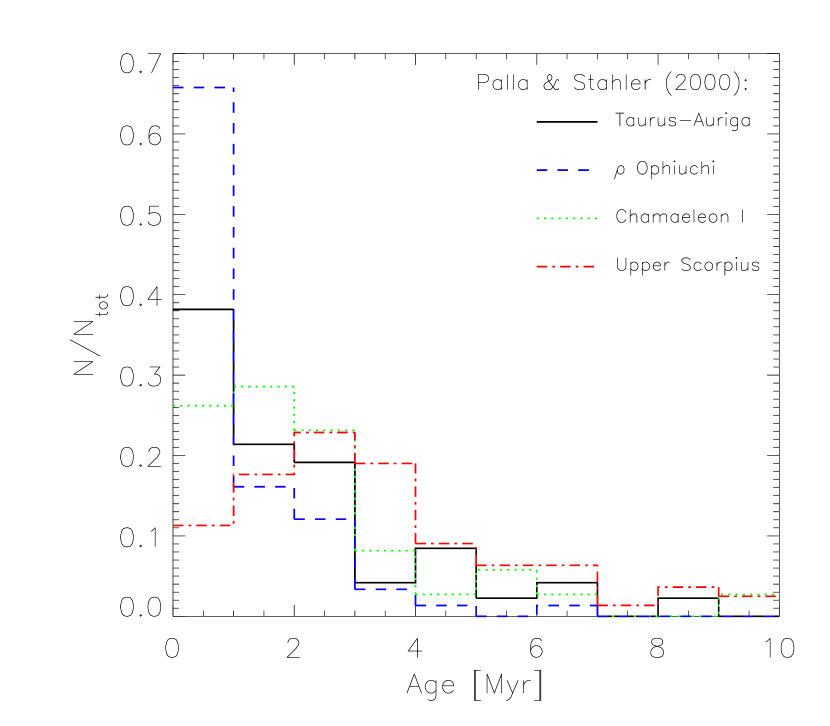
Figure 8: Left: Stellar age distribution for our calibrated model with $R_{\rm inf}=10$ pc ($M_{\rm max}\approx 2000{\rm M}_{\odot}$), calculated at the end of the cloud’s evolution. Right: Compilation of the age histograms for the associations studied by Palla & Stahler (2000).

These results can be compared with the age histograms presented by Palla & Stahler (2000) for the Orion Nebula Cluster (ONC), the Taurus-Auriga region, Lupus, $\rho$-Oph, Chameleon, Upper Scorpius, and IC348. In these clusters, the fraction of stars with ages up to 1 Myr ranges from $\sim 30$% to 66%, while the fraction of stars with ages up to 4 Myr is in the range 80 – 97%. Moreover, only in the case of Upper Scorpius does the age histogram peak at an age larger than 1 Myr, namely at 3 Myr. For this association, the fraction of stars with ages $\leq 1$ Myr is only 11%, while the fraction with ages $\leq 4$ Myr is 71%. We show a compilation of these in the right panel of Fig. 8.

We can see that, qualitatively, the stellar age histogram at the end of our model’s life resembles those of Palla & Stahler (2000), although, quantitatively, the model’s histogram in Fig. 8 is much more concentrated towards short ages. However, this must be due to the fact that it was calculated at the end of the model’s evolution. Clearly this is not the case for the clusters and groups analyzed by Palla & Stahler (2000), because, as those authors themselves point out, in most cases the clusters are still embedded in their parent clouds, with only Upper Scorpius being already exposed. This means that we should consider our model before the end of its life.

In Fig. 9 we show the age histogram for the calibrated model, calculated at 1 and 2 Myr before the end of its evolution, and compare it with one of the histograms from Palla & Stahler (2000) – that for $\rho$-Oph. We see that the histogram becomes less peaked as earlier times before the cloud’s destruction are taken, becoming more closely resemblant to the histograms of Palla & Stahler (2000). This is because, as the SFR increases towards later times, the fraction of young stars becomes increasingly larger. In particular, the histograms for 1 and 2 Myr before the cloud’s dispersal seem to bracket the histogram for $\rho$-Oph. As seen from the right panel of Fig. 8, the other regions are less concentrated towards short ages. According to our model, then, $\rho$ Oph is a somewhat more evolved region, well matched by our model at $\lesssim 2$ Myr before its dispersal, while the other regions would correspond to somewhat less evolved stages, at slightly earlier times (3–4 Myr) before destruction.

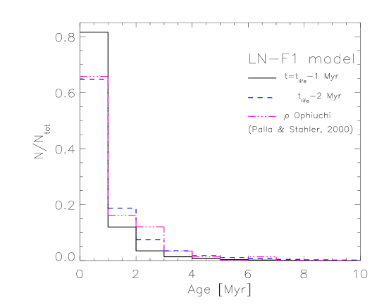
Figure 9: Stellar age distribution for our calibrated model with $R_{\rm inf}=10$ pc ($M_{\rm max}\approx 2000{\rm M}_{\odot}$), calculated at one and two Myr before the end of the cloud’s evolution, compared with the corresponding distribution for the $\rho$-Oph association (Palla & Stahler, 2000).

These results suggest a possible resolution of the debate between the Palla-Stahler and the Hartmann groups. Specifically, although our model indeed predicts an increase of the SFR in collapsing clouds, this does not conflict with the conundrum posed by Hartmann (2003): no fully formed molecular clouds are observed without significant amounts of star formation because the clouds themselves are evolving. Thus, at the time when they had much lower SFRs, they were not fully formed yet, and thus not identifiable as large molecular clouds. Indeed, the clouds’ mean density was lower, and thus, in reality, they probably consisted of a few molecular clumps immersed in a still-atomic interclump medium. Only in the last few Myr of their evolution, the clouds are dense enough on average that most of their bulk is already molecular, and by that time they are forming stars at a much higher rate, as observed. A similar conclusion has been recently reached on the basis of numerical simulations by Hartmann et al. (2012).

6 Discussion

6.1 The constant-$\mathcal{M}_{\rm rms}$ assumption

A feature of our model that may appear odd at first sight is that we have taken $\mathcal{M}_{\rm rms}=3$ as the (constant) fiducial value for the rms Mach number of the turbulence within the cloud, as it is contrary, for example, to the famous Larson (1981) velocity dispersion-size scaling relation. However, it must be recalled that in this paper we are specifically assuming that such a relation, or its more modern rendition by Heyer et al. (2009), is a manifestation of the gravitational contraction of the cloud, rather than a feature of the turbulence (Ballesteros-Paredes et al., 2011). Thus, the relevant rms Mach number must be the remainder after the collapsing motions have been removed. A competition may be set up between the transfer of kinetic energy from the collapsing motions to the turbulent ones and the dissipation (Vázquez-Semadeni et al., 1998; Klessen & Hennebelle, 2010), and so, in the absence of a reliable model, we consider that the assumption of a constant rms Mach number with the value typical for the CNM (Heiles & Troland, 2003) is reasonable, although a possible alternative recipe for its initial value would be to take it equal to the inflow Mach number (Banerjee et al., 2009). We consider that further work is necessary to better constrain this parameter.

6.2 The lognormal PDF assumption

A similar situation arises for the density PDF in the cloud, which we have assumed to have a lognormal shape, even though it is well known that star-forming clouds develop a power-law tail at high densities (Klessen, 2000; Dib & Burkert, 2005; Vázquez-Semadeni et al., 2008; Kainulainen et al., 2009; Kritsuk et al., 2011; Ballesteros-Paredes et al., 2011b). However, Kritsuk et al. (2011) have suggested that such power-law tails are the effect of the development of local collapsing sites with power-law density profiles. In this case, as explained in §2.5, the power-law tail in the PDF would be the result of the collapse, rather than the seed for it, and thus the relevant PDF for the seeds for future collapse should be the underlying lognormal one, after removal of the already-collapsing regions. Moreover, there is no complete theory for how the density PDF should evolve in time from a lognormal to a power-law. Unknowns such as the timescale for the transition, the density at which the power-law tail starts, and the final slope of this region are uncertain at present. As above, we consider that further work is necessary to clearly resolve this issue, and in the meantime we settle for the lognormal PDF assumption.

6.3 Accelerating star formation

An important precision is in order concerning the acceleration of star formation in our model. Indeed, our model predicts that the star formation rate increases over time, and therefore, star formation (SF; strictly speaking, the instantaneous stellar mass, $M_{\rm S}(t)$) accelerates. However, it is common to find the statement in the literature that it is the SFR that accelerates. This is not the case for our model with feedback. The SFR is the time derivative of $M_{\rm S}$. Since the SFR increases in time, the second time derivative of $M_{\rm S}$ is positive, and thus the SF accelerates. However, the second time derivative of the SFR (the third derivative of $M_{\rm S}$) is negative for our model with feedback (see the left panel of Fig. 4), and thus strictly speaking the SFR decelerates.

6.4 Room for improvement

In the present model, we have bypassed the supporting effect of all forms of pressure, and replaced it by the empirical “Larson factor”, $f_{\rm L}$, which effectively lengthens the timescale for collapse. In the case of the original work by Larson (1969, Appendix C), this factor represented the support from thermal pressure which, incidentally, should be most important during the earlier stages of the collapse. Calibrating against the SAF1 simulation by Vázquez-Semadeni et al. (2010), we found a value of $f_{\rm L}$ rouhly 8% larger than the one found by Larson, suggesting perhaps that turbulent pressure added a certain (small) amount of support (the magnetic field was not included in that simulation). Including physically-motivated terms into the collapse prescription that account for thermal, turbulent and magnetic support is an important goal, which we will attempt to pursue in a future contribution.

Nevertheless, it is interesting that our model, calibrated in the non-magnetic case of the SAF1 simulation, gives a good match to a number of observational properties of molecular clouds in a wide range of masses. This suggests that magnetic support is not crucial in these objects. In turn, this is consistent with the recent realization that star-forming clouds tend to be magnetically supercritical in general (Bourke et al., 2001; Crutcher et al., 2003; Troland & Crutcher, 2008), and thus they should be essentially in a free-fall regime.

Finally, in this paper we have not considered the effect of supernova explosions towards the late evolutionary stages of the clouds. This may help in reducing the model’s SFR at those stages, probably bringing it to better agreement with the observations (cf. Fig. 7).

7 Summary and Conclusions

In this paper we have developed a semi-empirical analytical model (based on simulations by Vázquez-Semadeni et al., 2010) in which a MC is formed by converging WNM flows. We assumed that the inflow collision produces a CNM cloud, through nonlinear triggering of the thermal instability, and that the cloud becomes turbulent through the combined action of the latter and various other dynamical instabilities, such as the nonlinear thin shell, Kelvin-Helmholtz, and Rayleigh-Taylor ones. We assumed that the rms Mach number of this turbulence remains fixed at the typical values in the CNM ($\mathcal{M}_{\rm s}\approx 3$), and that over its evolution, the cloud develops further nonthermal motions related to its collapse, not its internal turbulence. We also assumed that the cloud forms stars with a Kroupa (2001)-type IMF, so that massive stars only appear when a sufficiently large number of stars has formed to adequately sample the high-mass tail of the IMF. Finally, we assumed that the density PDF in the cloud has a lognormal shape and a fixed width (corresponding to a constant turbulent Mach number $\mathcal{M}_{\rm rms}$), but whose maximum shifts towards higher densities as the cloud contracts and becomes denser on average.

Using the same WNM inflow parameters as the simulation labeled SAF1 from Vázquez-Semadeni et al. (2010), namely $R_{\rm inf}=64\,{\rm pc}$, $n_{\rm inf}=1~{}{\rm cm}^{-3}$, and $\mathcal{M}_{\rm rms}=3$, we calibrated the model by searching the density threshold for star formation, $n_{\rm SF}$, that best matched the simulation’s evolution of the SFR and SFE. Our calibrated value was $n_{\rm SF}=10^{6}~{}{\rm cm}^{-3}$. With the $n_{\rm SF}$, $n_{\rm inf}$, and $\mathcal{M}_{\rm rms}$ parameters fixed, the only remaining free parameter of the model is the WNM inflow radius $R_{\rm inf}$, which essentially controls the maximum mass reached by the model cloud, $M_{\rm max}$. Varying this parameter we then match the model to clouds of various masses, and compare with various properties of such clouds.

The generic behavior of the model cloud, with the parameters of the SAF1 simulation, are as follows: i) The size of the model cloud decreases faster (by gravitational contraction) in a case without stellar feedback (model LN-F0) than in a case with it (model LN-F1). This is because feedback partially evaporates the cloud, thus reducing its gravitational potential, and slowing its collapse. ii) The model without feedback approaches a final state of zero size with finite mass (a singularity), while the case with feedback approaches a final state of zero mass at finite size; i.e., it is completely consumed by SF and ionization before if reaches zero size. iii) Although the SFR increases in both cases, it accelerates over time in the LN-F0 model, while it decelerates over time in the LN-F1 model.

We then set out to apply the model to explain a number of observed features of molecular clouds of a wide range of masses. First, we compared the predictions of our model with the evolutionary scenario for GMCs recently proposed by Kawamura et al. (2009), in which the GMCs start out having no massive stars, then have reduced numbers of them, so as to only have isolated HII regions, and finally have large numbers of them, so as to clearly contain massive clusters. We find that our model, with a value of $R_{\rm inf}$ that gives $M_{\rm max}\sim 10^{5}~{}{\rm M}_{\odot}$, comparable to the mass range reported by those authors, spends similar times in each of the stages reported by them.

We also investigated a model cloud with $R_{\rm inf}=10$ pc, corresponding to $M_{\rm max}\sim 2000~{}{\rm M}_{\odot}$. We find that such a model cloud evolves in the $\Sigma_{\rm SFR}$-$\Sigma_{\rm gas}$, or Kennicutt-Schmidt, diagram, in such a way that it passes first through the locus of individual low-mass-star forming clouds and later through the locus of high-mass-star forming clumps, as reported by Evans et al. (2009) and Heiderman et al. (2010). Next, we compared an evolved stage of the calibrated model, also using $R_{\rm inf}=10$ pc, with the physical conditions in the OMC-1 massive clump, finding that it has similar physical conditions after $\sim 26$ Myr of evolution since its parent molecular cloud first formed, although it spends only about 2 Myr in a state comparable to OMC-1.

Finally, we investigated the stellar age distribution in our isolated-cloud model with $R_{\rm inf}=10$ pc, showing that, taken a few Myr before the end of the cloud’s life, it is consistent with the corresponding distributions presented by Palla & Stahler (2000) for various clusters and associations. Furthermore, the model predicts that the shape of this age distribution depends on the evolutionary stage of the system, being more peaked towards young ages as the system grows older, because of its increasing SFR.

We conclude that our evolutionary and collapsing model of molecular clouds adequately represents actual clouds of a wide range of masses, with no need whatsoever for the consideration of equilibrium states. In this sense, the present model, although idealized, represents a promising first attempt at a non-equilibrium model for molecular clouds and their star-forming properties.

References

- Ballesteros-Paredes & Hartmann (2007) Ballesteros-Paredes, J., & Hartmann, L. 2007, Rev. Mexicana Astron. Astrofis., 43, 123
- Ballesteros-Paredes et al. (2011) Ballesteros-Paredes, J., Hartmann, L. W., Vázquez-Semadeni, E., Heitsch, F., & Zamora-Avilés, M. A. 2011, MNRAS, 411, 65
- Ballesteros-Paredes et al. (2011b) Ballesteros-Paredes,J., Vázquez-Semadeni, E., Gazol, A., et al. 2011b, MNRAS, 416, 1436
- Bally et al. (1987) Bally, J., Lanber, W. D., Stark, A. A., & Wilson, R. W. 1987, ApJ, 312, L45
- Banerjee et al. (2009) Banerjee, R., Vázquez-Semadeni, E., Hennebelle, P., & Klessen, R. S. 2009, MNRAS, 398, 1082
- Bate et al. (1995) Bate, M. R., Bonnell, I. A., & Price, N. M. 1995, MNRAS, 277, 362
- Bigiel et al. (2008) Bigiel, F., Leroy, A., Walter, F., et al. 2008, AJ, 136, 2846
- Bigiel et al. (2010) Bigiel, F., Leroy, A., & Walter, F. 2010, Proceedings IAU Symposium No. 270, 2010
- Bourke et al. (2001) Bourke, T. L., Myers, P. C., Robinson, G., & Hyland, A. R. 2001, ApJ, 554, 916
- Burkert & Hartmann (2004) Burkert, A., & Hartmann, L. 2004, ApJ, 616, 288
- Clark & Bonnell (2005) Clark, P. C., & Bonnell, I. A. 2005, MNRAS, 361, 2
- Crutcher et al. (2003) Crutcher, R., Heiles, C., & Troland, T. 2003, Turbulence and Magnetic Fields in Astrophysics, 614, 155
- Csengeri et al. (2010) Csengeri, T., Bontemps, S., Schneider, N., Motte, F., & Dib, S. 2010, A&A, 527, 135
- Dib & Burkert (2005) Dib, S., & Burkert, A. 2005, ApJ, 630, 238
- Dib et al. (2011) Dib, S., Piau, L., Mohanty, S., & Braine, J. 2011, MNRAS, 415, 3439
- Elmegreen (2002) Elmegreen, B. G. 2002, ApJ, 577, 206
- Evans et al. (2009) Evans, N. J., et al. 2009, ApJS, 181, 321
- Federrath, Klessen & Schmidt (2008) Federrath, C., Klessen, R. S., & Schmidt, W. 2008, ApJ, 688, L79
- Federrath et al. (2010) Federrath, C., Banerjee, R., Clark, P. C., & Klessen, R. S. 2010, ApJ, 713, 269
- Franco, Shore & Tenorio-Tagle (1994) Franco, J., Shore, S. N., & Tenorio-Tagle, G. 1994, ApJ 436, 795
- Folini & Walder (2006) Folini, D., & Walder, R. 2006, A&A, 459,1
- Galván-Madrid et al. (2009) Galván-Madrid, R., Keto, E., Zhang, et al. 2009, ApJ, 706, 1036
- Galván-Madrid et al. (2007) Galván-Madrid, R., Vázquez-Semadeni, E., Kim, J., & Ballesteros-Paredes, J. 2007, ApJ, 670, 480
- Goldbaum et al. (2011) Goldbaum, N. J., Krumholz, M. R., Matzner, C. D., & McKee, C. F. 2011, ApJ, 738, 101
- Goldreich & Kwan (1974) Goldreich, P., & Kwan, J. 1974, ApJ 189, 441
- Hartmann (2003) Hartmann, L. 2003, ApJ, 585, 398
- Hartmann, Ballesteros-Paredes, & Bergin (2001) Hartmann, L., Ballesteros-Paredes, J., & Bergin, E. A. 2001, ApJ, 562, 852
- Hartmann et al. (2012) Hartmann, L., Ballesteros-Paredes, J., & Heitsch, F. 2012, MNRAS, 420, 1457
- Hartmann & Burkert (2007) Hartman, L., & Burkert, A., 2007, ApJ, 654, 988.
- Heiderman et al. (2010) Heiderman, A., Evans, N. J., II, Allen, L. E., Huard, T., & Heyer, M. 2010, ApJ, 723, 1019
- Heiles & Troland (2003) Heiles, C., & Troland, T. H. 2003, ApJ, 586, 1067
- Heitsch et al. (2005) Heitsch, F., Burkert, A., Hartmann, L., Slyz, A. D., & Devriendt, J. E. G. 2005, ApJ 633, L113
- Heitsch et al. (2006) Heitsch, F., Slyz, A., Devriendt, J., Hartmann, L., & Burkert, A. 2006, ApJ, 648, 1052
- Heitsch & Hartmann (2008) Heitsch, F., & Hartmann, L. 2008, ApJ, 689, 290
- Hennebelle & Pérault (1999) Hennebelle, P., & Pérault, M. 1999, A&A, 351, 309
- Heyer et al. (2009) Heyer, M., Krawczyk, C., Duval, J., & Jackson, J. M. 2009, ApJ, 699, 1092
- Hunter et al. (1986) Hunter, J. H., Jr., Sandford, M. T., II, Whitaker, R. W., & Klein, R. I. 1986, ApJ, 305, 309
- Kainulainen et al. (2009) Kainulainen, J., Beuther, H., Henning, T., & Plume, R. 2009, A&A, 508, L35
- Kawamura et al. (2009) Kawamura, A., Mizuno, Y., Minamidani, T., et al. 2009, ApJS, 184, 1
- Kennicutt (1998b) Kennicutt, R. C., Jr. 1998b, ApJ, 498, 541
- Klessen (2000) Klessen, R. S. 2000, ApJ, 535, 869
- Klessen & Hennebelle (2010) Klessen, R. S., & Hennebelle, P. 2010, A&A, 520, A17
- Koyama & Inutsuka (2000) Koyama H., & Inutsuka S. I., 2000 ApJ, 532, 980
- Koyama & Inutsuka (2002) Koyama, H., & Inutsuka, S.-I. 2002, ApJ, 564, L97
- Kritsuk et al. (2011) Kritsuk, A. G., Norman, M. L., & Wagner, R. 2011, ApJ, 727, L20
- Kroupa (2001) Kroupa, P. 2001, MNRAS, 322, 231
- Krumholz & McKee (2005) Krumholz, M. R., & McKee, C. F. 2005, ApJ, 630, 250
- Krumholz et al. (2006) Krumholz, M. R., Matzner, C. D., & McKee, C. F. 2006, ApJ, 653, 361
- Larson (1969) Larson, R. B. 1969, MNRAS, 145, 271
- Larson (1981) Larson, R. B. 1981, MNRAS, 194, 809
- Larson (1985) Larson, R. B. 1985, MNRAS, 214, 379
- Leisawitz et al. (1989) Leisawitz, D., Bash, F. N., & Thaddeus, P. 1989, ApJS, 70, 731
- Li & Nakamura (2006) Li, Z.-Y., & Nakamura, F. 2006, ApJ, 640, L187
- Mac Low & Klessen (2004) Mac Low, M. -M. & Klessen, R. S. 2004, Rev. Mod. Phis., 76, 125
- Matzner (2002) Matzner, C. D. 2002, ApJ, 566, 302
- McKee (1989) McKee, C. F. 1989, ApJ, 345, 782
- McKee & Ostriker (2007) McKee, C. F., & Ostriker, E. C. 2007, ARA&A, 45, 565
- Nakamura & Li (2007) Nakamura, F., & Li, Z.-Y. 2007, ApJ, 662, 395
- Norman & Silk (1980) Norman, C., & Silk, J. 1980, ApJ, 238, 158
- Padoan et al. (1997) Padoan, P., Nordlund, A., & Jones, B. J. T. 1997, MNRAS, 288, 145
- Palla & Stahler (1999) Palla, F., & Stahler, S. W. 1999, ApJ, 525, 772
- Palla & Stahler (2000) Palla, F., & Stahler, S. W. 2000, ApJ, 540, 255
- Palla & Stahler (2002) Palla, F., & Stahler, S. W. 2002, ApJ, 581, 1194
- Passot & Vázquez-Semadeni (1998) Passot, T. & Vázquez-Semadeni, E. 1998, Phys. Rev. E, 58, 4501
- Peretto, Hennebelle & André (2007) Peretto, N., Hennebelle, P., & André, P. 2007, A&A, 464, 983
- Penston (1969) Penston, M. V. 1969, MNRAS, 144, 425
- Pon et al. (2011) Pon, A., Johnstone, D., & Heitsch, F. 2011, ApJ, 740, 88
- Rosas-Guevara et al. (2010) Rosas-Guevara, Y., Vázquez-Semadeni, E., Gómez, G. C., & Jappsen, A. -K. 2010, MNRAS, 406, 1875
- Schmidt (1959) Schmidt, M. 1959, ApJ, 129, 243
- Schneider et al. (2010) Schneider, N., Csengeri, T., Bontemps, et al. 2010, A&A, 520, A49
- Shu (1977) Shu, F. H. 1977, ApJ, 214, 488
- Troland & Crutcher (2008) Troland, T. H., & Crutcher, R. M. 2008, ApJ, 680, 457
- Vázquez-Semadeni (1994) Vázquez-Semadeni, E. 1994, ApJ, 423, 681
- Vázquez-Semadeni et al. (1998) Vazquez-Semadeni, E., Canto, J., & Lizano, S. 1998, ApJ, 492, 596
- Vázquez-Semadeni et al. (2006) Vázquez-Semadeni, E., Ryu, D., Passot, T., González, R. F., & Gazol, A. 2006, ApJ, 643, 245
- Vázquez-Semadeni et al. (2007) Vázquez-Semadeni, E., Gómez, G. C., Jappsen, A. K., et al. 2007, ApJ, 657, 870
- Vázquez-Semadeni et al. (2008) Vázquez-Semadeni, E., González, R. F., Ballesteros-Paredes, J., Gazol, A., & Kim, J. 2008, MNRAS, 390, 769
- Vázquez-Semadeni et al. (2009) Vázquez-Semadeni, E., Gómez, G. C., Jappsen, A.-K., Ballesteros-Paredes, J. & Klessen, R. S. 2009, ApJ, 707, 1023
- Vázquez-Semadeni et al. (2010) Vázquez-Semadeni, E., Colín, P., Gómez, G. C., Ballesteros-Paredes, J., & Watson, A. W. 2010, ApJ, 715, 1302
- Vázquez-Semadeni et al. (2011) Vázquez-Semadeni, E., Banerjee, R., Gómez G. C., et al. 2011, MNRAS, 414, 2511
- Vishniac (1994) Vishniac E. T. 1994, ApJ, 428, 186
- Walder & Folini (2000) Walder, R., & Folini, D. 2000, ApSS, 274, 343
- Wang et al. (2010) Wang, P., Li, Z.-Y., Abel, T., & Nakamura, F. 2010, ApJ, 709, 27
- Wu et al. (2005) Wu, J., Evans, N. J., II, Gao, Y., et al. 2005, ApJ, 635, L173
- Wu et al. (2010) Wu, J., Evans, N. J., Shirley, Y. L., & Knez, C. 2010, ApJS, 188, 313
- Zuckerman & Evans (1974) Zuckerman B., & Evans N. J. 1974, ApJ, 192, L149
- Zuckerman & Palmer (1974) Zuckerman, B., & Palmer, P. 1974, ARA&A, 12, 279