Hadron multiplicity induced by top quark decays at the LHC.

Abstract

The average charged hadron multiplicities induced by top quark decays are calculated in pQCD at LHC energies. Different modes of top production are considered. Proposed measurements can be used as an additional test of pQCD calculations independent on a fragmentation model.

1 Introduction

The study of unstable heavy particles like W, Z bosons, top quarks and others (arising in different extensions of the Standard Model) is one of the leading directions in the modern high energy physics. To determine particle parameters (charge, mass, width, decay modes etc.) we have to look deep inside their production and decay mechanisms.

In this article processes with top production are considered due to its specific properties. Top quark is extremely elusive object. Because its mass is so large ($m_{t}^{exp}=172\pm 0.9\pm 1.3\;{\rm GeV}$) PDG2010 , it can decay into on-shell W-bosons, i.e., the two-particle decay mode $t\to bW^{+}$ is kinematically possible. The SM predicts the top quark to decay almost exclusively into this mode. The on-shell W-boson can then decay leptonically or hadronically with coupling strengths given by the Cabibo-Kobayashi-Maskawa (CKM) matrix. The top quark decay proceeds extremely fast, in less than $\tau_{t}=1/\Gamma_{t}\simeq 5\times 10^{-25}\;{\rm s}$, which is shorter than the time scale to form hadrons $\tau_{had}\simeq 1/\Lambda_{QCD}\approx 3\times 10^{-24}\;{\rm s}$ and almost 13 orders of magnitude smaller than the lifetime of hadrons, which involve the next heaviest quark, $\tau_{b}\simeq 1.5\times 10^{-12}\;{\rm s}$. The width $\Gamma_{t}$ acts as a physical ”smearing”, and the top production becomes a quantitative prediction of pQCD, largely independent on nonperturbative phenomenological algorithms. That is why top measurements are directly related to pQCD tests.

The principal observables used in tests of pQCD are typically measurements of jets, high transverse momentum particles and event shapes. There are relative advantages and disadvantages in using these observables. Jet measurements are expected to have a close correlation in direction and momentum with the parton which gave rise to it. However, several complications concerning jet definitions (algorithms) arise when using jet measurements. While the infrared and collinear safety of event shapes allows safe perturbative predictions, we have to take into account resummation of large logarithms. Evolution of structure functions can be predicted by pQCD calculations, but we have to consider different kinematical regimes (see, for example, recent review on QCD tests QCDtests ). The transition from partons to hadrons cannot be accomodated within perturbative QCD. Fragmentation mechanism is usually simulated by the use of additional approaches (string fragmentation, cluster fragmentation). It was shown PK1 ; PK2 that measurements of average charged hadron multiplicitiy in a jet (especially jet produced in heavy quark decay) can serve as a precise test of pQCD independent on a fragmentation model.

Measurements of quark and gluon jets show visible differences between them. For example, gluon jets are fatter, softer and have higher multiplicity ellis1988 . In events induced by heavy quark jets the hadron multiplicity is smaller than in analogous events triggered by light quark jets picsmult1 -picsmult3 . The situation is similar to the classical theory, where the more is the mass of a charged particle, the less intensive is the radiation from it. The dependence of the multiplicity in a quark jet on the ”primary quark” mass was observed in previous experiments, in particular, at the SLC, KEK, LEPI and LEPII (see PK3 and references therein). Leading order pQCD predicts ”specific scaling” PK1 ,PK3 -scaling1 , i.e. energy independent difference between average charged multiplicities of light and heavy quark jets. The advantage of multiplicity measurement is that we do not need large number of events, and it can be used in rare processes like, for example, single top production.

The QCD radiation associated with $t\bar{t}$ production has been treated earlier in ttrad1 ; ttrad2 . These papers consider the effect, that gluons are also radiated from the b’s from t-decay. This effect has been also taken into account here. Recently top production at the ILC $e^{+}e^{-}$ collider was considered PK2 . Following the basic idea of Ref. PK2 it is possible to analyse the case of top production at the LHC. Since in pp events the energy of parton interaction is not fixed and changes in the range from about 400 GeV up to several TeV, we can study the evolution of average multiplicities in this energy domain. Of course, several obvious difficulties can arise (color interconnection, interference effects). It is shown, that there are some cases where we can successfully avoid the above complications.

The paper is organized as follows. In the first section there is an outlook of the basic model. The second one is devoted to numerical results for different mechanisms of the top production at the LHC. Complicated formulae and calculations are collected in Appendices.

2 Model

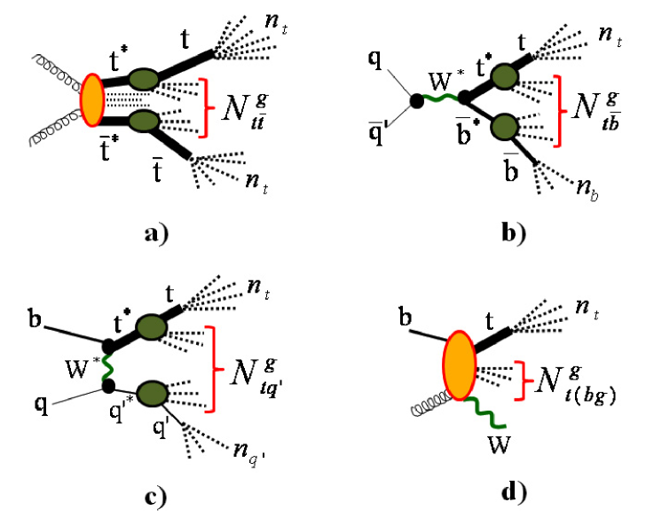
Figure 1: Parton level processes of top production at LHC considered in this paper: a) dominant $t\bar{t}$ production in the gluon-gluon fusion; b) s-channel single top production; c) t-channel single top production; d) tW production.

The model used in this section is analogous to the one presented in PK1 . In this article we consider processes of the type $p+p\to t\bar{t}+X$ or $p+p\to t+X$ (see Fig. 1). The basic formula for inclusive production of the system $M$ in the collinear approximation looks as follows

$$\frac{d\sigma_{pp\to M\;X}(s)}{dx_{1}dx_{2}d\Phi_{M}}=\sum_{i,j}f_{i}(x_{1})f_{j}(x_{2})\frac{d\hat{\sigma}_{ij\to M}}{d\Phi_{M}}(x_{1}x_{2}s;\ \{\Phi_{M}\}),$$ (1)

where $f_{i}(x)$ is the probability to find parton $i$ (quark, anti-quark or gluon) with the longitudinal momentum $x\sqrt{s}/2$ in a proton. Renormalization and factorization scales are hidden in $f$ and $\hat{\sigma}$. Here M is the system of different final states like $t\bar{t}$, $t\bar{b}$, $tq$, $tW$, which corresponds to different mechanisms of the inclusive top production at the LHC. $X$ includes beam remnants ($X_{beam}$) and also the secondary radiation induced by color interactions inside M ($X_{M}$) plus possible interaction between M and beam remnants ($X_{M-beam}$), if M is not a color singlet. Variables $x_{1,2}$ are fixed in every separate event and can be calculated experimentally. Usually the sum in (1) can be approximated by a single factorized term which includes parton distributions multiplied by the amplitude squared of parton-parton cross-sections:

$$g+g\to t\bar{t}+X_{M}\mbox{(dominates at the LHC)},$$ (2)

$$q+\bar{q}^{\prime}\to W^{*}\to t\bar{b}+X_{M},$$ (3)

$$b+q\to tq^{\prime}+X_{M},$$ (4)

$$b+g\to tW+X_{M},$$ (5)

$$q+g\to t\bar{b}q^{\prime}+X_{M},$$ (6)

$$g+g\to t\bar{b}W+X_{M},$$ (7)

where $q,\;q^{\prime}$ denotes corresponding light quarks. For our purposes it is enough to consider initial parton collisions instead of pp process, since we have to calculate only the charged hadron multiplicity of the $M$ plus $X_{M}$ in a separate event. Complications concerning $X_{beam}$ and $X_{M-beam}$ are discussed below. $X_{M}$ comes from virtual gluon radiation.

For the average multiplicity of hadrons in $M+X_{M}$ we can use the expression similar to Eq. (5) in PK1 :

$$N_{M+X_{M}}^{h}(Q^{2})=n_{M}+$$

$$\!\int\!\frac{d^{4}k}{(2\pi)^{4}}\,\Pi_{\mu\nu}^{ab}(q_{1},q_{2},k)\,d^{\,\mu\alpha}_{aa^{\prime}}(k)\,d^{\,\nu\beta}_{bb^{\prime}}(k)\,n^{a^{\prime}b^{\prime}}_{\alpha\beta}(k)\;,$$ (8)

where $d^{\,\mu\nu}_{ab}(k)\equiv i\;\tilde{d}^{\,\mu\nu}_{ab}(k)/(k^{2}+i0)$ is the propagator of the gluon with momentum $k$, $q_{1,2}$ are momenta of initial partons. Here and below $(a,b)$ and $(a^{\prime},b^{\prime})$ denote color indices, $Q=\sqrt{(q_{1}+q_{2})^{2}}$ is the energy of colliding partons.

The first term in the r.h.s. of Eq. (8), $n_{M}$, is the multiplicity from the fragmentation of leading particles in the final state. For example, in the process (2) $n_{M}=n_{t\bar{t}}=2n_{t}$, where $n_{t}$ was calculated in PK2 . In other processes $n_{M}$ is appropriate combination of multiplicities which are taken from the analysis of data and pQCD calculations:

$$n_{t}^{H}\equiv n_{t}(t\to{\rm hadrons})=41.03\pm 0.54\mbox{\cite[cite]{\@@bibref{Authors Phrase1YearPhrase2}{PK2}{\@@citephrase{(}}{\@@citephrase{)}}}},$$ (9)

$$n_{t}^{L}\equiv n_{t}(t\to l\bar{\nu}_{l}+{\rm hadrons})=21.9\pm 0.53\mbox{\cite[cite]{\@@bibref{Authors Phrase1YearPhrase2}{PK2}{\@@citephrase{(}}{\@@citephrase{)}}}},$$ (10)

$$n_{W}(W\to{\rm hadrons})=19.34\pm 0.10\mbox{\cite[cite]{\@@bibref{Authors Phrase1YearPhrase2}{PK2}{\@@citephrase{(}}{\@@citephrase{)}}}}$$ (11)

$$n_{c}=2.6,\;n_{b}=5.5\mbox{\cite[cite]{\@@bibref{Authors Phrase1YearPhrase2}{dataMULTbc}{\@@citephrase{(}}{\@@citephrase{)}}}},\;n_{q}=1.2\mbox{\cite[cite]{\@@bibref{Authors Phrase1YearPhrase2}{dataMULTq}{\@@citephrase{(}}{\@@citephrase{)}}}}.$$ (12)

Tensor $n^{a^{\prime}b^{\prime}}_{\alpha\beta}(k)$ is given in PK1 :

$$n^{a^{\prime}b^{\prime}}_{\alpha\beta}(k)=\left(-g_{\alpha\beta}\,k^{2}+k_{\alpha}k_{\beta}\right)\delta^{a^{\prime}b^{\prime}}n_{g}(k^{2})\;,$$ (13)

where dimensionless quantity $n_{g}(k^{2})$ describes the average multiplicity of hadrons in the gluon jet with the virtuality $k^{2}$. It is, of course, gauge invariant, and depends only on the virtuality $k^{2}$.

The quantity $n_{g}(k^{2})$ cannot be calculated perturbatively. It is usually assumed that the average hadron multiplicity is proportional to $n_{g}(k^{2},Q_{0}^{2})$, i.e. the average multiplicity of (off-shell) partons with the “mass” $Q_{0}$ (the so-called local parton-hadron duality):

$$n_{g}(k^{2})=n_{g}(k^{2},Q_{0}^{2})\,K(Q_{0}^{2})\;,$$ (14)

where $K(Q_{0}^{2})$ is a phenomenological energy-independent factor. The QCD evolution equations for both $n_{g}(k^{2},Q_{0}^{2})$ and

$$N_{g}(k^{2},Q_{0}^{2})=\int\limits_{Q_{0}^{2}}^{k^{2}}\frac{dp^{2}}{p^{2}}n_{g}(p^{2},Q_{0}^{2})$$ (15)

are derived in PK1 , and also in old works eqNg1 ; eqNg2 . We use the “conventional standard” value $Q_{0}=1\;{\rm GeV}$ for further numerical calculations. Here $N_{g}(k^{2},Q_{0}^{2})$ is the average multiplicity from the gluon jet whose virtuality $p^{2}$ varies up to $k^{2}$. Very often $N_{g}$ is erroneously called the average multiplicity of the gluon jet with fixed virtuality $k^{2}$. This meaning should be addressed to $n_{g}$ only.

In this paper we will use two phenomenological expressions (to estimate theoretical uncertainties) for $n_{g}$ which can be found in PK1 :

$$n^{i}_{g}(k^{2}) \!= \!k^{2}\frac{d}{dk^{2}}N^{i}_{g}(k^{2},Q_{0}^{2}),$$ (16)

$$\!\!\!N^{1}_{g}(k^{2}) \!= \!3.89+0.01\exp\left[1.63\sqrt{\ln\left(\frac{k^{2}}{\Lambda_{1}^{2}}\right)}\right],$$

$$\Lambda_{1} \!= \!0.87\;{\rm GeV}\mbox{\rm(QCD motivated)},$$ (17)

$$\!\!\!N^{2}_{g}(k^{2}) \!= \!4.21+0.012\ln^{2}\frac{k^{2}}{\Lambda_{2}^{2}},\;\Lambda_{2}=0.93\;{\rm GeV}.$$ (18)

Parameters for these functions were obtained in PK2 (see eq.(3) and Fig.8 in this reference, where $n_{g}$ corresponds to the function $N_{g}$ in the present paper) by the fitting of the data from scaling1 .

In Eq. (8) the first factor of the integrand is given by

$$\Pi_{\mu\nu}^{ab}(q_{1},q_{2},k)=\left[\prod_{i=1}^{N_{in.gl.}}\tilde{d}^{\rho_{i}\sigma_{i}}(q_{i},n)\delta_{a_{i}b_{i}}\right]\times$$

$$\phantom{\Pi_{\mu\nu}^{ab}(q_{1},q_{2},k)=\left[\right.}\Pi_{\{\rho_{i}\sigma_{i}\};\;\mu\nu}^{\{a_{i}b_{i}\};\;ab}(q_{1},q_{2},k)\;,$$ (19)

where $\Pi_{\{\rho_{i}\sigma_{i}\};\;\mu\nu}^{\{a_{i}b_{i}\};\;ab}(q_{1},q_{2},k)$ can be calculated in the first order in the strong coupling constant as the amplitude squared of the corresponding process (2)-(7) with $X_{M}=g$ normalized to the total rate of the process without $X_{M}$. Sum in the product of polarization vectors of initial gluons ($N_{in.gl.}=0,1,2$) forms usual factor (here we use the axial gauge since it simplifies much theoretical calculations)

$$\tilde{d}^{\rho_{i}\sigma_{i}}(q_{i},n) \!= \!\sum_{\lambda=1,2}\epsilon_{(i);\lambda}^{\rho_{i}}\epsilon_{(i);\lambda}^{*;\sigma_{i}}=$$

$$-g^{\rho_{i}\sigma_{i}} \!+ \!\frac{q_{i}^{\rho_{i}}n^{\sigma_{i}}+n^{\rho_{i}}q_{i}^{\sigma_{i}}}{qn}-\frac{n^{2}}{qn^{2}}q_{i}^{\rho_{i}}q_{i}^{\sigma_{i}},$$ (20)

where $\epsilon_{(i);\lambda}^{\rho}q_{i;\rho}=0$, $q_{i}^{2}=0$, $n$ is an appropriate four-vector in the corresponding process (see Appendices B,C).

The quantity (19) satisfies the equality

$$k^{\mu}\Pi_{\mu\nu}^{ab}(q_{1},q_{2},k)=0$$ (21)

due to the general theorem Predazzigauge : If the QCD amplitude is written

$$\!\!\!\!\!\!\!\!\!\!\mathcal{A}_{QCD}=$$

$$\!\!\!\!\!\!\!\!\!\!\epsilon_{\nu_{1}}^{\star}(\kappa_{1})...\epsilon_{\nu_{N}}^{\star}(\kappa_{N})\,\mathcal{T}_{a_{1}...a_{N}\,;\,\,b_{1}...b_{M}}^{\nu_{1}...\nu_{N}\,;\,\,\mu_{1}...\mu_{M}}\,\epsilon_{\mu_{1}}(k_{1})...\epsilon_{\mu_{M}}(k_{M})$$ (22)

then one gets zero if any number, $\geq 1$, of the polarization vectors $\epsilon_{\mu_{j}}(k_{j})$ and/or $\epsilon^{*}_{\nu_{i}}(\kappa_{i})$ are replaced by $k_{j\,,\,\mu_{j}}$ and/or $\kappa_{i\,,\,\nu_{i}}$ respectively, provided that all these $k_{j}$’s and $\kappa_{i}$’s, with the exception of at most one of them , satisfy $k_{j}^{2}=0$ and $\kappa_{i}^{2}=0$.

If we take into account Eq. (21) and introduce the function

$$\Pi(Q^{2},k^{2},kq_{1},kq_{2})=(-g^{\mu\nu})\delta_{ab}\Pi_{\mu\nu}^{ab}(Q^{2},k^{2},kq_{1},kq_{2}),$$ (23)

the final formula for the multiplicity will look as follows:

$$N_{M+X_{M}}^{h}(Q^{2})=n_{M}+N^{g}_{M}\equiv$$

$$n_{M}+\!\int\!\frac{d^{4}k}{(2\pi)^{4}}\,\Pi(Q^{2},k^{2},kq_{1},kq_{2})\left.\frac{d}{dp^{2}}N_{g}(p^{2})\right|_{p^{2}=k^{2}}.$$ (24)

Concrete form of the function $\Pi$ for different processes can be found in Appendices B,C.

3 Numerical results of calculations

In this section we consider numerical results for average charged multiplicities in different processes of top production at the LHC. Below we consider the phase space when final jets have low transverse momentum cuts $P_{t}$, and the final gluon jet can not be experimentally separated from one of final quark jets (i.e. gluon jet lies within the cone $\cos\theta_{gq}>R=0.9$, where $\theta_{gq}<0.45$ is the angle between the gluon and quark jets).

Table 1: Multiplicity $N^{g}_{t\bar{t}}$ for different cuts of jet transverse momenta $P_{t}$ and the energy of gluon-gluon collision.

$N^{g}_{t\bar{t}}(Q,P_{t})$	$Q$, GeV
$P_{t}$, GeV	600	1000	1500
10	2.82$\pm$0.07	8.29$\pm$0.2	15.75$\pm$0.36
30	0.76$\pm$0.02	2.96$\pm$0.06	6.58$\pm$0.12
50	0.4$\pm$0.01	1.3$\pm$0.02	3.63$\pm$0.05

Let us begin with the inclusive $t$ $\bar{t}$ production (2). The total cross-section of the inclusive process $pp\to t\bar{t}+X$ is about 833 pb at 14 TeV. In this article we consider only the gluon-gluon fusion mechanism of this process since at LHC it is dominant. Numerical values for $N^{g}_{t\bar{t}}$ are given in the table 1 and on the Fig. 2. Here and below theoretical errors are estimated by the use of two different parametrizations (17),(18) for the hadronic multiplicity in a gluon jet. The average charged multiplicity in different decay modes (hadronic, semileptonic and leptonic) can be calculated as follows

$$N^{h}_{t\bar{t}\to hadrons}(Q) \!= \!2n^{H}_{t}+N^{g}_{t\bar{t}}(Q),$$ (25)

$$N^{h}_{t\bar{t}\to l\bar{\nu}_{l}+hadrons}(Q) \!= \!n^{H}_{t}+n_{t}^{L}+N^{g}_{t\bar{t}}(Q),$$ (26)

$$N^{h}_{t\bar{t}\to l^{+}l^{-}\nu_{l}\bar{\nu}_{l}+hadrons}(Q) \!= \!2n_{t}^{L}+N^{g}_{t\bar{t}}(Q).$$ (27)

As you see on the Fig. 2, the dependence of $N^{g}_{t\bar{t}}$ on the energy is visible. In this work we assume that color reconnection of $t\bar{t}$ and beam remnants is small due to the strong suppression of this processes with high transverse momentum transfer (typical jet transverse momentum cut at the LHC is about $20$-$40$ GeV). Also $t$ and $\bar{t}$ fragment independently after the interaction inside the $t\bar{t}$ system. It looks similar to the process of $W^{+}W^{-}$ fragmentation in $e^{+}e^{-}$ annihilation. The effect of possible color reconnection was investigated by comparing hadronic multiplicities in $e^{+}e^{-}\to W^{+}W^{-}\to q\bar{q}^{\prime}q\bar{q}^{\prime}$ and $e^{+}e^{-}\to W^{+}W^{-}\to q\bar{q}^{\prime}l\bar{\nu}_{l}$. No evidence for final state interactions was found by measuring the difference $<n_{4q}^{h}>-2<n_{2ql\bar{\nu}}^{h}>$ WWfragm1 ,WWfragm2 . The values for average charged multiplicities can be compared with the present LHC data on the inclusive $t\bar{t}$ production.

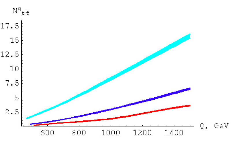
Figure 2: $t\bar{t}$ production. Multiplicity $N^{g}_{t\bar{t}}$ versus $Q$ for different cuts of jet transverse momenta. Top-down: $P_{t}=10\;GeV\to P_{t}=30\;GeV\to P_{t}=50\;GeV$.

Table 2: S-channel single top production. Multiplicity $N^{g}_{t\bar{b}}$ for different cuts of jet transverse momenta $P_{t}$ and the energy of parton-parton collision.

$N^{g}_{t\bar{b}}(Q,P_{t})$	$Q$, GeV
$P_{t}$, GeV	600	1000	1500
10	11$\pm$0.32	14.8$\pm$0.41	18.7$\pm$0.5
30	6.55$\pm$0.19	10$\pm$0.27	13.2$\pm$0.33
50	4.33$\pm$0.12	7.55$\pm$0.2	10.4$\pm$0.25

The case of s-channel single top production (3) is close to the $e^{+}e^{-}$ one, since the final state is a result of $W$ decay, i.e. color singlet. That is why we have no color reconnection with beam remnants. However, the cross-section of this process is rather small (about 11 pb at 14 TeV), and the experimental task on the extraction of the multiplicity looks more difficult than, for example, in t-channel single top or $t\bar{t}$ production. Numerical values for $N^{g}_{t\bar{b}}$ are given in the table 2 and on the Fig. 3. The average charged multiplicity in different decay modes can be calculated as follows

$$N^{h}_{t\bar{b}\to hadrons}(Q) \!= \!n^{H}_{t}+n_{b}+N^{g}_{t\bar{b}}(Q),$$ (28)

$$N^{h}_{t\bar{b}\to l\bar{\nu}_{l}+hadrons}(Q) \!= \!n^{L}_{t}+n_{b}+N^{g}_{t\bar{b}}(Q).$$ (29)

The energy dependence is not so strong as in the previous case (see Fig. 3).

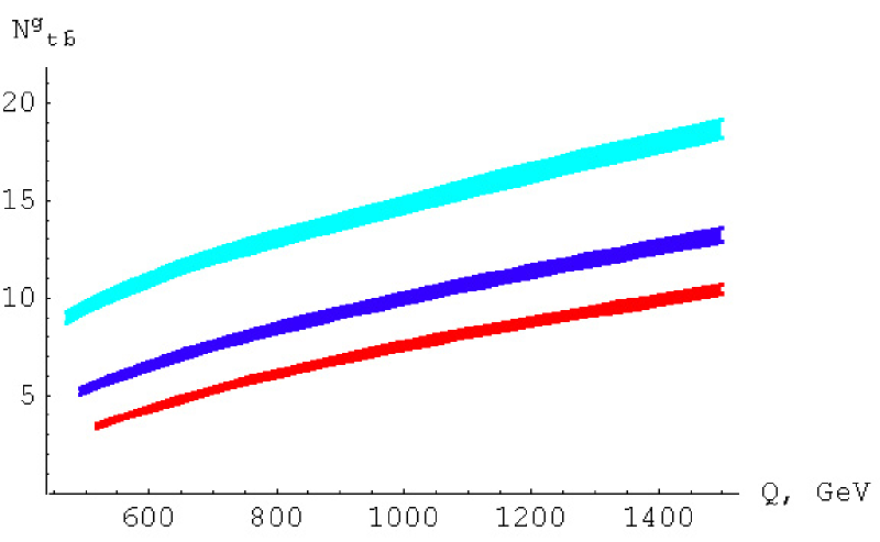
Figure 3: S-channel single top production. Multiplicity $N^{g}_{t\bar{b}}(Q)$ versus $Q$ for different cuts of jet transverse momenta. Top-down: $P_{t}=10\;GeV\to P_{t}=30\;GeV\to P_{t}=50\;GeV$.

Table 3: T-channel single top production. Multiplicity $N^{g}_{tq^{\prime}}$ for different cuts of jet transverse momenta $P_{t}$ and the energy of parton-parton collision.

$N^{g}_{tq^{\prime}}(Q,P_{t})$	$Q$, GeV
$P_{t}$, GeV	600	1000	1500
10	6.23$\pm$0.18	7.65$\pm$0.22	8.62$\pm$0.24
30	2.4$\pm$0.07	2.77$\pm$0.075	3.29$\pm$0.08
50	1.32$\pm$0.038	1.59$\pm$0.04	1.76$\pm$0.044

The process of t-channel single top production $pp\to t+X$ has higher rate (about 245 pb at 14 TeV) than the previous one, but we have to make the same assumptions concerning fragmentation and color reconnection processes as in $t\bar{t}$ production. Here calculations for the parton level process (4) are presented. Numerical values for $N^{g}_{tq^{\prime}}$ are given in the table 3 and on the Fig. 4.

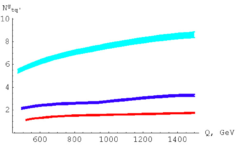
Figure 4: T-channel single top production. Multiplicity $N^{g}_{tq^{\prime}}(Q)$ versus $Q$ for different cuts of jet transverse momenta. Top-down: $P_{t}=10\;GeV\to P_{t}=30\;GeV\to P_{t}=50\;GeV$.

The average charged multiplicity in different decay modes looks as follows

$$N^{h}_{tq^{\prime}\to hadrons}(Q) \!= \!n^{H}_{t}+n_{q}+N^{g}_{tq^{\prime}}(Q),$$ (30)

$$N^{h}_{tq^{\prime}\to l\bar{\nu}_{l}+hadrons}(Q) \!= \!n^{L}_{t}+n_{q}+N^{g}_{tq^{\prime}}(Q).$$ (31)

Table 4: Multiplicity $N^{g}_{tW}$ for different cuts of jet transverse momenta $P_{t}$ and the energy of parton-parton collision.

$N^{g}_{tW}(Q,P_{t})$	$Q$, GeV
$P_{t}$, GeV	600	1000	1500
10	2.54$\pm$0.06	5.83$\pm$0.14	10.27$\pm$0.23
30	0.85$\pm$0.017	2.27$\pm$0.04	4.49$\pm$0.076
50	0.42$\pm$0.008	1.25$\pm$0.019	2.6$\pm$0.036

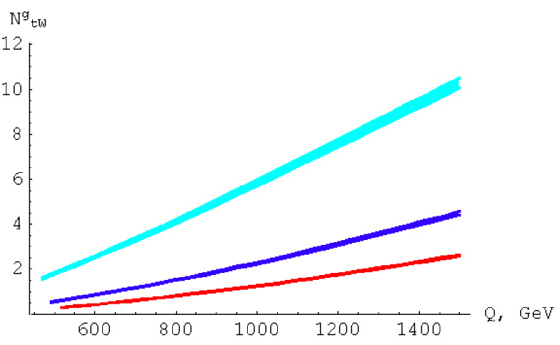
Figure 5: Multiplicity $N^{g}_{tW}(Q)$ versus $Q$ for different cuts of jet transverse momenta. Top-down: $P_{t}=10\;GeV\to P_{t}=30\;GeV\to P_{t}=50\;GeV$.

As you can see on the Fig. 4, the value of $N^{g}_{tq^{\prime}}$ is rather small in the wide kinematical region, and energy dependence is not strong. It is important for the estimation of the multiplicity from beam remnants plus color reconnection effects, since values $n_{t}^{H}$, $n_{t}^{L}$, $n_{q}$ are fixed by previous measurements and $N^{g}_{tq^{\prime}}(Q)\ll n_{t}$. From this point of view the t-channel single top production looks the most interesting process for the multiplicity measurements.

$tW$ production has intermediate cross-section of the order 62 pb at 14 TeV which lies between s- and t-channel single top production rates. Probably, specific signature of this process would help in the measurements proposed in this work. Numerical values for $N^{g}_{tW}$ are given in the table 4 and on the Fig. 5. The process (5) has 3 decay modes. The corresponding average charged multiplicities are

$$N^{h}_{tW\to hadrons}(Q) \!= \!n^{H}_{t}+n_{W}+N^{g}_{tW}(Q),$$ (32)

$$N^{h}_{tW\to(W)l\bar{\nu}_{l}+hadrons}(Q) \!= \!n^{H}_{t}+N^{g}_{tW}(Q),$$ (33)

$$N^{h}_{tW\to l^{+}l^{-}\nu_{l}\bar{\nu}_{l}+hadrons}(Q) \!= \!n^{L}_{t}+N^{g}_{tW}(Q).$$ (34)

The energy dependence is also visible and can be used to test QCD calculations.

4 Discussions and conclusions

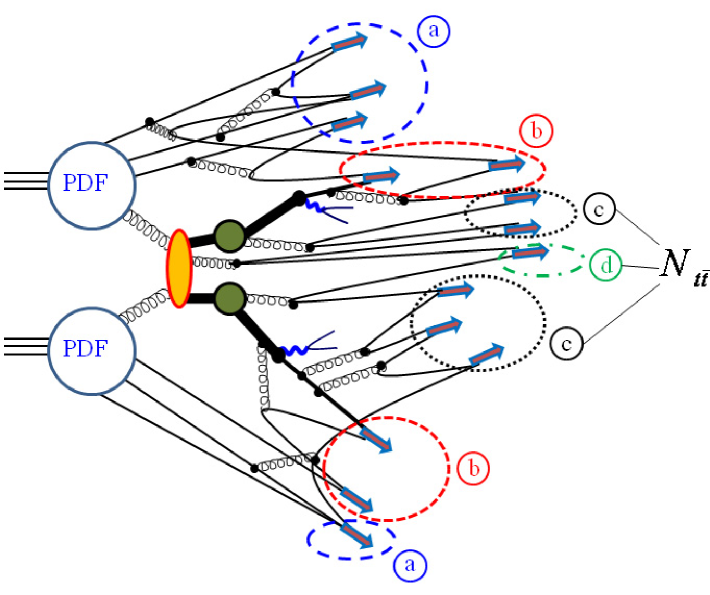
Figure 6: Complicated fragmentation pattern of the inclusive $t\bar{t}$ production in pp collisions. a) beam remnants; b) hadrons arising from the color interaction of beam remnants with the final state radiation from quarks (suppressed for high-$P_{t}$ of final quarks or gluons); c) hadrons from top fragmentation; d) result of $t^{*}\bar{t}^{*}$ interaction.

In this article we consider four processes with top production at the LHC. Average charged hadronic multiplicities were calculated in perturbative QCD. Hadronic multiplicity in a gluon is fixed by low energy data.

There are several important tasks that could be solved by multiplicity measurements: to test QCD calculations independently on fragmentation models, to check independent fragmentation of heavy quarks, to check parton-parton C.M. energy dependence of hadron multiplicities, to estimate multiplicity from beam remnants plus from color reconnection effects in t-channel single top for further use in other processes. We can calculate also the difference $\Delta N_{Qq}\equiv N_{Q}-N_{q}$ to cancel effects of color reconnection and beam remnants.

There are several assumptions in the present work:

• independent fragmentation of on-shell top quarks in $t\bar{t}$ production;

• color reconnection effects in the interaction of jets with beam remnants (for nonsinglet production of $t\bar{t}$, $tq^{\prime}$, $tW$) are suppressed for large lower cuts in jet transverse momenta. As you can see on the Fig. 6, the fragmentation pattern in $t\bar{t}$ production is rather complicated. We have beam remnants with low transverse momenta interacting with jet remnants with large transverse momenta. Amplitudes for such processes are suppressed for high $P_{t}$ since they are propotional to the inverse power of the momentum transfer squared $\hat{t}$ in the parton-parton interaction, and

  $$\hat{t} \!= \!(p^{beam}_{0}-p^{jet}_{0})^{2}-(p^{beam}_{3}-p^{jet}_{3})^{2}-$$

  $$(\vec{p}^{\;beam}_{t}-\vec{p}^{\;jet}_{t})^{2}\simeq-{p^{jet}_{t}}^{2}<-P_{t}^{2},$$

  where $p^{beam}$ and $p^{jet}$ are momenta of beam and jet partons correspondingly, and from the kinematics

  $$p^{beam}_{0}\sim|p^{beam}_{3}|\gg p^{jet}_{0}\sim|p^{jet}_{3}|,\ p^{jet}_{t}\gg p^{beam}_{t}.$$

  We are interested only in c and d types of fragmentation depicted on the Fig. 6.

• in the s-channel $t\bar{b}$ singlet production there is no color reconnection with beam remnants.

All the above assumptions are based on low energy data and theoretical estimations of pQCD and also can bechecked at the LHC.

From the experimental point of view t-channel single top production (4) is the most convenient case, since the energy dependence of the average charged hadronic multiplicity is weak. We can estimate quantitatively effect of color reconnection of jets with beam remnants to check our assumption on its suppression. Then we can use this estimation to improve our predictions for other channels of top production. For this task it is also useful to extract multiplicities in different decay modes of top quarks.

The final experimental task is to extract number of tracks in jets which are produced in top quark decays. To estimate experimental efficiencies and dependence on a fragmentation model we can use any MC generator for top production. At the same time with the top-mass reconstruction procedure (in hadronic mode) we could extract number of tracks which are included into hadronic cluster from single top or top anti-top decays. At the moment we have a good chance to make the new independent test of QCD by the use of recent LHC data at $7$ TeV. Other experimental aspects of such measurements will be discussed in futher works.

Appendix A

Let us consider the process

$$parton_{1}(q_{1})+parton_{2}(q_{2})\to c(p_{1})+d(p_{2})+g(k)$$ (35)

and put $q_{i}^{2}=0$, $k^{2}=K^{2}>0$ (we put also $m_{b}=0$ for processes (5),(6), since corrections are of the order $m_{b}^{2}/m_{t}^{2}\ll 1$). In the C.M. frame of colliding partons we can write:

$$q_{1}=\frac{Q}{2}\left(1,0,0,1\right),\;q_{2}=\frac{Q}{2}\left(1,0,0,-1\right),$$

$$q=q_{1}+q_{2},\;\Delta=(q_{1}-q_{2})/2,$$ (36)

$$k=\left(\frac{qk}{Q},\frac{\sqrt{D}}{Q}\sin\theta_{k},0,\frac{\sqrt{D}}{Q}\cos\theta_{k}\right),$$

$$l=\left(\frac{Q^{2}+Z}{2Q},|{\vec{l}\;\!}|\sin\theta_{l}\cos\phi,|{\vec{l}\;\!}|\sin\theta_{l}\sin\phi,|{\vec{l}\;\!}|\cos\theta_{l}\right),$$

$$p_{1}=l-k,\;p_{2}=q-l,$$ (37)

$$D=(qk)^{2}-Q^{2}K^{2},\;|{\vec{l}\;\!}|=\sqrt{\frac{\left(Q^{2}-Z\right)^{2}}{4Q^{2}}-m_{2}^{2}},$$

$$\hat{s}=(q-k)^{2}=Q^{2}+K^{2}-2qk,\;Z=l^{2}-m_{2}^{2},$$ (38)

$$\cos\theta_{kl}=\cos\theta_{k}\cos\theta_{l}+\sin\theta_{k}\sin\theta_{l}\cos\phi\;\;\;\;\;\mbox{\rm or}$$

$$\cos\theta_{l}=\cos\theta_{kl}\cos\theta_{k}+\sin\theta_{kl}\sin\theta_{k}\cos\phi^{*}.$$ (39)

After change of variables phase space looks as follows:

$$\int dK^{2}\int d\Phi_{2\to 3}=\int dK^{2}\int\!\!\!\!\int\frac{d^{4}k}{(2\pi)^{4}}\frac{d^{4}l}{(2\pi)^{4}}\times$$

$$(2\pi)\delta(p_{1}^{2}-m_{1}^{2})(2\pi)\delta(p_{2}^{2}-m_{2}^{2})(2\pi)\delta(K^{2}-k_{\mu}k^{\mu})=$$

$$\left[\frac{\sqrt{D}}{2(2\pi)^{2}Q^{2}}\int\!\!\!\!\int\!\!\!\!\int dK^{2}\;d(qk)\;d\cos\theta_{k}\right]\times$$

$$\left[\int\!\!\!\!\int\!\!\!\!\int\frac{\delta(\mathcal{H}(Z))}{2(4\pi)^{2}\sqrt{D}}\;dZ\;d\phi\;d\cos\theta_{l}\right]=$$

$$\frac{1}{2(4\pi)^{3}Q^{2}}\int\limits_{K_{-}^{2}}^{K_{+}^{2}}dK^{2}\int\limits_{(qk)_{-}}^{(qk)_{+}}d(qk)\int\limits_{C_{k,-}}^{C_{k,+}}d\cos\theta_{k}\int\limits_{Z_{-}}^{Z_{+}}dZ\int\limits_{0}^{\pi}\frac{d\phi}{\pi},$$

$$\!\!\!\mathcal{H}(Z)=\cos\theta_{kl}(Z)-\cos\theta_{k}\cos\theta_{l}-\sin\theta_{k}\sin\theta_{l}\cos\phi.$$ (40)

Here we keep the integration in $K^{2}$ since the gluon is virtual.

Then we have to cut jet transverse momenta from below to suppress color reconnection with beam remnants

$$p_{i,\perp}\geq P_{t,i},\;k_{\perp}\geq K_{t},$$

or

$$p_{i,3}\leq\sqrt{\vec{p}_{i}^{2}-P_{t,i}^{2}},\;k_{3}\leq\sqrt{\vec{k}^{2}-K_{t}^{2}}.$$

In this paper $K_{t}=P_{t,i}=P_{t}$. Finally we have conditions

$$\left|\cos\theta_{l}\right|\left|\vec{l}\right|\leq\sqrt{\vec{l}^{2}-P_{t,2}^{2}},$$ (41)

$$\left|\left|\vec{l}\right|\cos\theta_{l}-\left|\vec{k}\right|\cos\theta_{k}\right|\leq\sqrt{\left(\vec{l}-\vec{k}\right)^{2}-P_{t,1}^{2}}.$$ (42)

For limits in the above integrals without conditions (41),(42) we can write

$$K_{-}^{2}=Q_{0}^{2},\;K_{+}^{2}=\left(Q-\sqrt{(m_{1}+m_{2})^{2}+K_{t}^{2}}\right)^{2}-K_{t}^{2},$$

$$(qk)_{-}=Q\sqrt{K^{2}+K_{t}^{2}},$$

$$(qk)_{+}=\frac{Q^{2}+K^{2}-(m_{1}+m_{2})^{2}}{2},$$

$$m_{i,\perp}=\sqrt{m_{i}^{2}+P_{t}^{2}},$$

$$C_{k,\pm}=\pm\sqrt{\frac{D-Q^{2}K_{t}^{2}}{D}},$$

$$Q\geq\sqrt{(m_{1}+m_{2})^{2}+K_{t}^{2}}+$$

$$\phantom{Q\geq}\;+\sqrt{Q_{0}^{2}+K_{t}^{2}}>m_{1}+m_{2}+Q_{0},$$

$$Q\leq x_{i,max}\sqrt{s}.$$ (43)

Taking into account the inequality ($\cos\theta_{kl}$ can be obtained from $\delta((k-l)^{2}-m_{1}^{2})$)

$$\left|\cos\theta_{kl}\right|=\left|-\frac{A_{l}}{\frac{Q}{2}|{\vec{l}\;\!}|}\right|\leq 1,$$ (44)

where

$$A_{l}=\frac{Q^{2}}{4\sqrt{D}}\left[K^{2}-qk+Z\left(1-\frac{qk}{Q^{2}}\right)+m_{2}^{2}-m_{1}^{2}\right]$$ (45)

and $|\vec{l}|$(see (39)) depend on $Z$, we can obtain limits:

$$\!\!\!\!Z_{\pm}=$$

$$\!\!qk+\frac{(Q^{2}-qk)(m_{1}^{2}-m_{2}^{2})}{\hat{s}}\pm\sqrt{D}\sqrt{D_{12}(\hat{s},m_{1},m_{2})},$$

$$\!\!\!\!D_{12}(s,m_{1},m_{2})=$$

$$\phantom{D_{12}}\!\left(1-\frac{(m_{1}+m_{2})^{2}}{s}\right)\left(1-\frac{(m_{1}-m_{2})^{2}}{s}\right).$$ (46)

For multidimensional integration it is convenient to introduce undimensional variables and make appropriate symmetrization of the function under the integration:

$$\phi=x_{\phi}\pi,\;x_{\phi}\in[0,1],$$

$$Z=qk+\frac{(Q^{2}-qk)(m_{1}^{2}-m_{2}^{2})}{\hat{s}}+$$

$$\zeta\sqrt{D}\sqrt{D_{12}(\hat{s},m_{1},m_{2})},\;\zeta\in[-1,1],$$

$$\cos\theta_{k}=\tau\sqrt{\frac{D-Q^{2}K_{t}^{2}}{D}},\;\tau\in[-1,1],$$

$$qk=(qk)_{-}+\eta((qk)_{+}-(qk)_{-}),\;\eta\in[0,1],$$ (47)

$$\int d(qk)\;d\cos\theta_{k}\;dZ\;\frac{d\phi}{\pi}\;f(qk,\cos\theta_{k},Z,\phi)=$$

$$\int\limits_{0}^{1}d\eta\;d\tau\;d\zeta\;dx_{\phi}\;\mathcal{D}\;\tilde{f}^{sym},$$ (48)

$$\tilde{f}^{sym} \!= \!\tilde{f}(\eta,\tau,\zeta,x_{\phi})+\tilde{f}(\eta,-\tau,\zeta,x_{\phi})+$$ (49)

$$\tilde{f}(\eta,\tau,-\zeta,x_{\phi})+\tilde{f}(\eta,-\tau,-\zeta,x_{\phi}),$$

$$\mathcal{D} \!= \!((qk)_{+}-(qk)_{-})\times$$ (50)

$$\sqrt{D-Q^{2}K_{t}^{2}}\sqrt{D_{12}(\hat{s},m_{1},m_{2})},$$

where $\tilde{f}$ is equal to $f$ after the change of variables.

In this paper we consider the case, when the final gluon jet can not be separated experimentally from one of final quark jets:

$$\cos\theta_{gq}>R=0.9,\;\mbox{or}\;\theta_{gq}<0.45.$$

The above inequality leads to the following conditions

$$\cos\theta_{\vec{p}_{2}\vec{k}} = -\cos\theta_{kl}>R,$$ (51)

$$\mbox{or}\;\cos\theta_{\vec{p}_{1}\vec{k}} = \left.-\cos\theta_{kl}\right|_{\zeta\to-\zeta}>R,$$ (52)

where $\cos\theta_{kl}$ is expressed in terms of variables $\zeta$, $\eta$, $x_{\phi}$, $\tau$.

Let us denote conditions (41),(42),(51),(52) as a product of corresponding $\theta$-functions

$$f_{T,R}=\theta\left(\sqrt{\vec{l}^{2}-P_{t,2}^{2}}-\left|\cos\theta_{l}\right|\left|\vec{l}\right|\right)\times$$

$$\theta\left(\sqrt{\left(\vec{l}-\vec{k}\right)^{2}-P_{t,1}^{2}}-\left|\left|\vec{l}\right|\cos\theta_{l}-\left|\vec{k}\right|\cos\theta_{k}\right|\right)\times$$

$$\left[\theta\left(-\cos\theta_{kl}-R\right)\;\mbox{or}\;\theta\left(-\left.\cos\theta_{kl}\right|_{\zeta\to-\zeta}-R\right)\right],$$ (53)

where

$$\theta(x)=\left\{{1,\;x\geq 0}\atop{0,\;x<0}\right.\;.$$

Now we can rewrite the second term in the r.h.s. of Ref.(24) as follows

$$\int\frac{d^{4}k}{(2\pi)^{4}}\,\Pi(Q^{2},k^{2},kq_{1},kq_{2})f_{T,R}\times$$

$$\,\,\,\,\;\left.\frac{d}{dp^{2}}N_{g}(p^{2})\right|_{p^{2}=k^{2}}=\frac{I_{1}}{I_{2}},$$ (54)

$$I_{1}=\frac{1}{2(4\pi)^{2}Q^{2}}\int\limits_{K_{-}^{2}}^{K_{+}^{2}}dK^{2}\;\alpha_{s}(K^{2})\left.\frac{d}{dp^{2}}N_{g}(p^{2})\right|_{p^{2}=K^{2}}\times$$

$$\,\,\,\,\;\int\limits_{(qk)_{-}}^{(qk)_{+}}d(qk)\int\limits_{C_{k,-}}^{C_{k,+}}d\cos\theta_{k}\int\limits_{Z_{-}}^{Z_{+}}dZ\int\limits_{0}^{\pi}\frac{d\phi}{\pi}\;f_{T,R}\;\tilde{\Pi}_{2\to 3},$$ (55)

$$I_{2}=\frac{\sqrt{D_{12}(Q^{2},m_{1},m_{2})}}{16\pi}\int\limits_{-C^{\prime}}^{+C^{\prime}}d\cos\theta_{q_{1}p_{1}}\tilde{\Pi}_{2\to 2},$$ (56)

$$C^{\prime 2}=\frac{D_{12}(Q^{2},m_{1,\perp},m_{2,\perp})}{D_{12}(Q^{2},m_{1},m_{2})},$$ (57)

where $\tilde{\Pi}_{2\to 3}$($\tilde{\Pi}_{2\to 2}$) is the amplitude squared of the corresponding process (2)-(5) with (without) gluon radiation, which is calculated in Appendices B,C. For simplicity we put all the coupling constants to unity in these quantities. Here $g_{s}=\sqrt{4\pi\alpha_{s}}$ is the QCD coupling constant. All tensors are contracted as in (19),(23).

Different kinematical invariants of the process (35) can be expressed in terms of $Q^{2}$, $K^{2}$, $qk$, $\cos\theta_{k}$, $Z$, $\phi$ (and then $Q^{2}$, $K^{2}$, $\eta$, $\tau$, $\zeta$, $x_{\phi}$):

$$q_{1}q_{2}=\frac{Q^{2}}{2},\;p_{1}p_{2}=\frac{\hat{s}-m_{1}^{2}-m_{2}^{2}}{2},\;$$

$$p_{1}q_{1}=\frac{Q^{2}+Z-2qk}{4}+\Delta l-\Delta k,$$

$$p_{1}q_{2}=\frac{Q^{2}+Z-2qk}{4}-\Delta l+\Delta k,$$

$$p_{2}q_{1}=\frac{Q^{2}-Z}{4}-\Delta l,\;p_{2}q_{2}=\frac{Q^{2}-Z}{4}+\Delta l,$$

$$p_{1}k=\frac{Z-K^{2}-m_{1}^{2}+m_{2}^{2}}{2},$$

$$p_{2}k=\frac{2qk-Z-K^{2}+m_{1}^{2}-m_{2}^{2}}{2},$$

$$q_{1}k=\frac{qk}{2}+\Delta k,\;q_{2}k=\frac{qk}{2}-\Delta k,$$

$$\Delta k=-\frac{\sqrt{D}}{2}\cos\theta_{k},$$

$$\Delta l=A_{l}\cos\theta_{k}-B_{l}\sin\theta_{k}\cos\phi,$$ (58)

$$\!\!\!\!A_{l}=$$

$$\!\!\!\!\zeta\frac{Q^{2}-qk}{4}\sqrt{D_{12}(\hat{s},m_{1,\perp},m_{2,\perp})}-\frac{\sqrt{D}}{4}\left(1-\frac{m_{1}^{2}-m_{2}^{2}}{\hat{s}}\right),$$

$$\!\!\!\!B_{l}=$$

$$\!\!\!\!\!\sqrt{\frac{Q^{2}}{4}|{\vec{l}\;\!}|^{2}-A_{l}^{2}}=\frac{Q\sqrt{\hat{s}}}{4}\sqrt{D_{12}(\hat{s},m_{1,\perp},m_{2,\perp})}\sqrt{1-\zeta^{2}}.$$ (59)

Appendix B

Here we consider amplitudes for the top-antitop production (2).

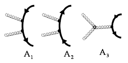
Figure 7: Amplitudes of the process $gg\to Q\bar{Q}$.

For the amplitude of the process without additional gluon radiation we have three diagrams of Fig. 7, and $I_{2}$ can be calculated as follows

$$\!\!\!I_{2} \!= \!\frac{8}{3\pi}\biggl{\{}8(1+4x_{m}^{2}+x_{m}^{4})\ln\frac{1+\sqrt{1-4x_{m\perp}^{2}}}{2x_{m\perp}}+$$ (60)

$$\!\!\!\!\sqrt{1-4x_{m\perp}^{2}}\left(3x_{m\perp}^{2}-18x_{m}^{2}-7-16\frac{x_{m}^{4}}{x_{m\perp}^{2}})\right)\biggr{\}},$$

$$x_{m}=m_{t}/Q,\;x_{m\perp}=m_{t,\perp}/Q.$$ (61)

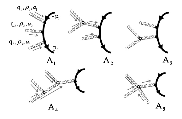
Figure 8: $gggQ\bar{Q}$ amplitudes.

For the amplitude of the process with additional gluon we have five kinds of diagrams (see Fig. 8):

$$A_{i}^{123}=\bar{u}(p_{2},m_{t})\hat{A}_{i}^{123}v(p_{1},m_{t}),$$ (62)

$$\hat{A}_{1}^{123}=[321]\frac{\gamma_{\rho_{3}}\left(\hat{p}_{2}-\hat{q}_{3}+m_{t}\right)\gamma_{\rho_{2}}\left(\hat{q}_{1}-\hat{p}_{1}+m_{t}\right)\gamma_{\rho_{1}}}{(q_{3}^{2}-2p_{2}q_{3})(q_{1}^{2}-2p_{1}q_{1})},$$

$$\hat{A}_{2}^{123}=\left([321]-[312]\right)\frac{\gamma_{\rho_{3}}\left(\hat{p}_{2}-\hat{q}_{3}+m_{t}\right)\gamma_{\lambda}}{(q_{3}^{2}-2p_{2}q_{3})}\frac{\tilde{d}^{\lambda\beta}(q_{1}+q_{2})}{(q_{1}+q_{2})^{2}}\times$$

$$\left\{(q_{1}-q_{2})_{\beta}g_{\rho_{1}\rho_{2}}-(2q_{1}+q_{2})_{\rho_{2}}g_{\beta\rho_{1}}+(2q_{2}+q_{1})_{\rho_{1}}g_{\beta\rho_{2}}\right\},$$

$$\hat{A}_{3}^{123}=\left([213]-[123]\right)\frac{\gamma_{\lambda}\left(\hat{q}_{3}-\hat{p}_{1}+m_{t}\right)\gamma_{\rho_{3}}}{(q_{3}^{2}-2p_{1}q_{3})}\frac{\tilde{d}^{\lambda\beta}(q_{1}+q_{2})}{(q_{1}+q_{2})^{2}}\times$$

$$\left\{(q_{1}-q_{2})_{\beta}g_{\rho_{1}\rho_{2}}-(2q_{1}+q_{2})_{\rho_{2}}g_{\beta\rho_{1}}+(2q_{2}+q_{1})_{\rho_{1}}g_{\beta\rho_{2}}\right\},$$

$$\hat{A}_{4}^{123}=\left([312]+[213]-[321]-[123]\right)\gamma_{\lambda}\frac{\tilde{d}^{\lambda\lambda^{\prime}}(p_{1}+p_{2})}{(p_{1}+p_{2})^{2}}\times$$

$$\left\{(2q_{3}-(p_{1}+p_{2}))_{\lambda^{\prime}}g_{\rho_{3}\beta^{\prime}}+(2(p_{1}+p_{2})-q_{3})_{\rho_{3}}g_{\lambda^{\prime}\beta^{\prime}}-\right.$$

$$\left.(q_{3}+(p_{1}+p_{2}))_{\beta^{\prime}}g_{\rho_{3}\lambda^{\prime}}\right\}\frac{\tilde{d}^{\beta^{\prime}\beta}(q_{1}+q_{2})}{(q_{1}+q_{2})^{2}}\times$$

$$\left\{(q_{1}-q_{2})_{\beta}g_{\rho_{1}\rho_{2}}-(2q_{1}+q_{2})_{\rho_{2}}g_{\beta\rho_{1}}+(2q_{2}+q_{1})_{\rho_{1}}g_{\beta\rho_{2}}\right\}$$

$$\hat{A}_{5}^{123}=\gamma_{\lambda}\frac{\tilde{d}^{\lambda\beta}(p_{1}+p_{2})}{(p_{1}+p_{2})^{2}}\times$$

$$\left\{\left([312]+[213]\right)\left(g_{\beta\rho_{2}}g_{\rho_{1}\rho_{3}}+g_{\beta\rho_{3}}g_{\rho_{1}\rho_{2}}-2g_{\beta\rho_{1}}g_{\rho_{2}\rho_{3}}\right)+\right.$$

$$\left.\left([321]+[123]\right)\left(g_{\beta\rho_{1}}g_{\rho_{2}\rho_{3}}+g_{\beta\rho_{3}}g_{\rho_{1}\rho_{2}}-2g_{\beta\rho_{2}}g_{\rho_{1}\rho_{3}}\right)+\right.$$

$$\left.\left([132]+[231]\right)\left(g_{\beta\rho_{1}}g_{\rho_{2}\rho_{3}}+g_{\beta\rho_{2}}g_{\rho_{1}\rho_{3}}-2g_{\beta\rho_{3}}g_{\rho_{1}\rho_{2}}\right)\right\},$$ (63)

where we consider all gluons as initial particles. Then we can calculate

$$\!\!\!\!\!\!\!\!\!\!T_{2\to 3\;\rho_{1}\rho_{2}\rho_{3}}^{\;\;\;\;\;\;\;a_{1}a_{2}a_{3}}(q_{1},q_{2},q_{3})=$$

$$\;\biggl{\{}A_{1}^{123}+A_{1}^{132}+A_{1}^{213}+A_{1}^{231}+A_{1}^{312}+A_{1}^{321}+$$

$$\;\;\;\sum_{i=2}^{4}\left(A_{i}^{123}+A_{i}^{132}+A_{i}^{231}\right)+A_{5}^{123}\biggr{\}},$$ (64)

$$\!\!\!\!\!\!\!\!\!\!\Pi^{\;\;\;\;\;\;\;\{a_{i}b_{i}\};ab}_{2\to 3\;\{\rho_{i}\sigma_{i}\};\mu\nu}=$$

$$\,T_{2\to 3\;\rho_{1}\rho_{2}\mu}^{\;\;\;\;\;\;\;a_{1}a_{2}a}(q_{1},q_{2},-k)T_{2\to 3\;\sigma_{1}\sigma_{2}\nu}^{*\;\;\;\;\;\;b_{1}b_{2}b}(q_{1},q_{2},-k).$$ (65)

Here $q_{3}=-k$ since we have one gluon in the final state with momentum $k$, $A_{i}^{123}\equiv A_{i\;\rho_{1}\rho_{2}\rho_{3}}^{\;\;a_{1}a_{2}a_{3}}(q_{1},q_{2},q_{3},p_{1,2})$, $[ijk]=t^{a_{i}}t^{a_{j}}t^{a_{k}}$, $t^{a}$ are SU(3) matrices, $u$ and $v$ are Dirac spinors, $\gamma_{\rho}$ are Dirac matrices, $\hat{p}\equiv p^{\mu}\gamma_{\mu}$.

If we apply contractions (19),(23) to (65) and take into account the theorem (22) (it was checked by direct calculations for (64) ) then we obtain $g_{s}^{6}\tilde{\Pi}_{2\to 3}$ for the process (2). Since the final expression for $\tilde{\Pi}_{2\to 3}$ is very complicated, we evaluate it numerically. To get the final result for the $t\bar{t}$ multiplicity induced by gluon radiation ($N^{g}_{t\bar{t}}$ on the Fig. 1a) we have to substitute $I_{2}$ and $\tilde{\Pi}_{2\to 3}$ for this process to (54)-(Appendix A).

Appendix C

For simplicity here we set all coupling constants to unity. In this section we consider calculations for processes (3)-(5).

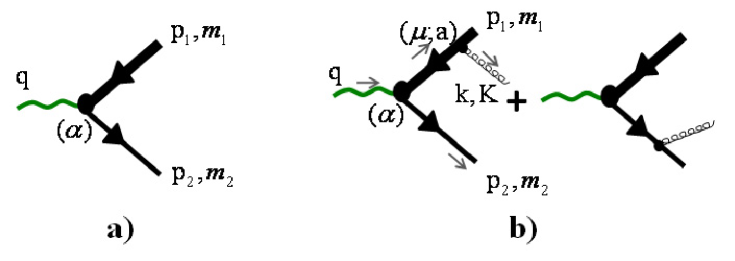
Figure 9: Amplitudes for calculation of functions $\mathcal{F}^{(0)}$ (a) and $\mathcal{F}^{(1)}$ (b).

Let us introduce some functions for futher calculations. One of the functions is the $WQ\bar{q}$ vertex squared (see Fig. 9a)

$$\mathcal{A}^{(0)}_{\alpha}=\bar{u}(p_{2},m_{2})\gamma_{\alpha}(1-\gamma_{5})v(p_{1},m_{1}),$$ (66)

$$\mathcal{F}^{(0)}_{\alpha\alpha^{\prime}}(p_{1},m_{1},p_{2},m_{2})=C_{A}\mathcal{A}^{(0)}_{\alpha}\mathcal{A}^{(0)\;*}_{\alpha^{\prime}}=$$

$$8C_{A}\biggl{(}g_{\alpha\alpha^{\prime}}p_{1}p_{2}-p_{1\;\alpha}p_{2\;\alpha^{\prime}}-p_{2\;\alpha}p_{1\;\alpha^{\prime}}-$$

$$\phantom{8C_{A}\biggr{(}}i\epsilon_{\alpha\alpha^{\prime}\rho\sigma}p_{1\;\rho}p_{2\;\sigma}\biggl{)}.$$ (67)

The next one is the squared amplitude of the process $W\to Q\bar{q}g$ which is shown on the Fig. 9b.

$$\mathcal{A}^{(1)}_{\alpha\mu}=\bar{u}(p_{2},m_{2})\left\{\frac{\gamma_{\alpha}(1-\gamma_{5})\left(-\hat{p}_{1}-\hat{k}+m_{1}\right)\gamma_{\mu}}{K^{2}+2p_{1}k}+\right.$$

$$\hskip 28.45274pt\left.\frac{\gamma_{\mu}\left(\hat{p}_{2}+\hat{k}+m_{2}\right)\gamma_{\alpha}(1-\gamma_{5})}{K^{2}+2p_{2}k}\right\}v(p_{1},m_{1}),$$ (68)

$$\mathcal{F}^{(1)}_{\alpha\alpha^{\prime}\;\mu\mu^{\prime}}(p_{1},m_{1},p_{2},m_{2},k,K)=C_{A}C_{F}\mathcal{A}^{(1)}_{\alpha\mu}\mathcal{A}^{(1)\;*}_{\alpha^{\prime}\mu^{\prime}},$$ (69)

$$\tilde{\mathcal{F}}^{(1)}_{\alpha\alpha^{\prime}}(p_{1},m,p_{2},0,k,K)=$$

$$\mathcal{F}^{(1)}_{\alpha\alpha^{\prime}\;\mu\mu^{\prime}}(p_{1},m,p_{2},0,k,K)\left(-g^{\mu\mu^{\prime}}+\frac{k^{\mu}k^{\mu^{\prime}}}{K^{2}}\right)=$$

$$\frac{128}{\left(K^{2}+2p_{1}k\right)^{2}\left(K^{2}+2p_{2}k\right)^{2}}\sum\limits_{i=1}^{9}\tilde{\mathcal{F}}^{(1);\;i}_{\alpha\alpha^{\prime}},$$ (70)

where

$$\tilde{\mathcal{F}}^{(1);\;1}_{\alpha\alpha^{\prime}}=g_{\alpha\alpha^{\prime}}\times$$

$$\biggl{\{}Q^{4}\left[Z(2qk-Z)+2m^{2}(Z-qk)-m^{4}\right]+$$

$$Q^{2}\left[-2K^{2}\left(m^{2}+qk-Z\right)^{2}-2qk(2qk-Z)Z-\right.$$

$$\hskip 8.5359pt\left.m^{2}(4qk-Z)Z+2m^{4}(qk-Z)+m^{6}\phantom{2K^{2}\left(m^{2}+qk-Z\right)^{2}}\right]+$$

$$K^{2}m^{2}\left[2qk^{2}-2Z\;qk+Z^{2}+2m^{2}(qk-Z)+m^{4}\right]+$$

$$Z(2qk-Z)(2qk^{2}-2Z\;qk+Z^{2})+$$

$$2m^{2}(-2qk^{3}+8qk^{2}Z-7Z^{2}qk+2Z^{3})+$$

$$2m^{4}(-3qk^{2}+7Z\;qk-3Z^{2})-4m^{6}(qk-Z)-m^{8}\biggr{\}},$$ (71)

$$\tilde{\mathcal{F}}^{(1);\;2}_{\alpha\alpha^{\prime}}=p_{1\;\alpha}p_{1\;\alpha^{\prime}}\times$$

$$\biggl{\{}K^{2}\left[-Z(2qk-Z)+2m^{2}(qk-Z)+m^{4}\right]+$$

$$Z(2qk-Z)^{2}-m^{2}(4qk^{2}-8Z\;qk+3Z^{2})-$$

$$m^{4}(4qk-3Z)-m^{6}\biggr{\}},$$ (72)

$$\tilde{\mathcal{F}}^{(1);\;3}_{\alpha\alpha^{\prime}}=p_{2\;\alpha}p_{2\;\alpha^{\prime}}\times$$

$$\biggl{\{}K^{2}\left[-Z(2qk-Z)+2m^{2}(qk-Z)+m^{4}\right]+$$

$$Z^{2}(2qk-Z)-m^{2}Z(4qk-3Z)+$$

$$m^{4}(2qk-3Z)+m^{6}\biggr{\}},$$ (73)

$$\tilde{\mathcal{F}}^{(1);\;4}_{\alpha\alpha^{\prime}}=\left(p_{1\;\alpha}p_{2\;\alpha^{\prime}}+p_{2\;\alpha}p_{1\;\alpha^{\prime}}\right)\times$$

$$\biggl{\{}Q^{2}\left[-Z(2qk-Z)+2m^{2}(qk-Z)+m^{4}\right]+$$

$$K^{2}\left[-Z(2qk-Z)+2m^{2}(qk-Z)+m^{4}+2qk^{2}\right]+$$

$$qk(2qk-Z)Z+2m^{2}qk^{2}+m^{4}qk\biggr{\}},$$ (74)

$$\tilde{\mathcal{F}}^{(1);\;5}_{\alpha\alpha^{\prime}}=\left(p_{1\;\alpha}k_{\alpha^{\prime}}+k_{\alpha}p_{1\;\alpha^{\prime}}\right)\times$$

$$\biggl{\{}\frac{Q^{2}}{2}\left[-Z(2qk-Z)+2m^{2}(qk-Z)+m^{4}\right]+$$

$$K^{2}\left[-Z(qk-Z)+m^{2}(qk-2Z)+m^{4}\right]+$$

$$\frac{1}{2}Z(2qk-Z)^{2}-m^{2}(qk-2Z)(2qk-Z)-$$

$$\frac{m^{4}}{2}(6qk-5Z)-m^{6}\biggr{\}},$$ (75)

$$\tilde{\mathcal{F}}^{(1);\;6}_{\alpha\alpha^{\prime}}=\left(p_{2\;\alpha}k_{\alpha^{\prime}}+k_{\alpha}p_{2\;\alpha^{\prime}}\right)\times$$

$$\biggl{\{}\frac{Q^{2}}{2}\left[-Z(2qk-Z)+2m^{2}(qk-Z)+m^{4}\right]+$$

$$K^{2}\left[2qk^{2}-3Z\;qk+Z^{2}+m^{2}(3qk-2Z)+m^{4}\right]+$$

$$\frac{1}{2}Z^{2}(2qk-Z)+m^{2}(4qk^{2}-5Z\;qk+2Z^{2})-$$

$$\frac{m^{4}}{2}(8qk-5Z)+m^{6}\biggr{\}},$$ (76)

$$\tilde{\mathcal{F}}^{(1);\;7}_{\alpha\alpha^{\prime}}=i\epsilon_{\alpha\alpha^{\prime}\sigma\rho}p_{1}^{\sigma}p_{2}^{\rho}\times$$

$$\biggl{\{}Q^{2}\left[-Z(2qk-Z)+2m^{2}(qk-Z)+m^{4}\right]+$$

$$K^{2}\left[2qk^{2}-3Z\;qk+Z^{2}+m^{2}(3qk-2Z)+m^{4}\right]+$$

$$Z(2qk-Z)(qk-Z)+m^{2}(2qk^{2}+4Z\;qk-3Z^{2})+$$

$$m^{4}(3Z-qk)-m^{6}\biggr{\}},$$ (77)

$$\tilde{\mathcal{F}}^{(1);\;8}_{\alpha\alpha^{\prime}}=i\left(\epsilon_{\alpha\sigma\rho\lambda}\mathcal{P}_{\alpha^{\prime}}-\epsilon_{\alpha^{\prime}\sigma\rho\lambda}\mathcal{P}_{\alpha}\right)k^{\sigma}p_{1}^{\rho}p_{2}^{\lambda},$$ (78)

$$\mathcal{P}_{\alpha}=\left(k-p_{1}+p_{2}\right)_{\alpha}\left(Z^{2}-2Z+m^{4}\right)+$$

$$\phantom{\mathcal{P}_{\alpha}=(}2qk(Z-m^{2})p_{1\;\alpha}$$ (79)

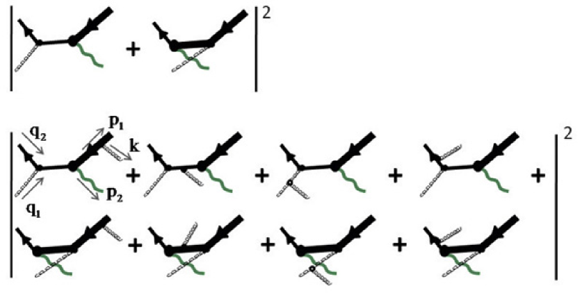
Figure 10: Diagrams for calculation of the process (5) and the tensor $\mathcal{F}^{(2)}$.

$$\tilde{\mathcal{F}}^{(1);\;9}_{\alpha\alpha^{\prime}}=i\epsilon_{\alpha\alpha^{\prime}\sigma\rho}k^{\sigma}p_{2}^{\rho}\times$$

$$\biggl{\{}Q^{2}\left[-Z(qk-Z)+m^{2}(qk-2Z)+m^{4}\right]+$$

$$K^{2}\left[2qk^{2}-3Z\;qk+Z^{2}+m^{2}(3qk-2Z)+m^{4}\right]+$$

$$m^{2}\left[4qk^{2}-Z\;qk-Z^{2}+m^{2}(qk+2Z)-m^{4}\right]\biggr{\}},$$ (80)

$$Z=l^{2}=(p_{1}+k)^{2}=(q-p_{2})^{2},\;m=m_{t}.$$

And the last one is the amplitude squared of the process which is depicted in the lower Fig. 10

$$\mathcal{F}^{(2)}_{\alpha\alpha^{\prime}\;\mu\mu^{\prime}\;\rho\rho^{\prime}}(p_{1},m_{1},q_{1},m^{\prime}_{1},q_{2},m^{\prime}_{2},k,K)=$$

$$\hskip 11.38092pt\left(\sum\limits_{i=1}^{8}\mathcal{A}^{(2)\;i}_{\alpha\mu\rho}\right)\left(\sum\limits_{j=1}^{8}\mathcal{A}^{(2)\;j}_{\alpha^{\prime}\mu^{\prime}\rho^{\prime}}\right)^{*},\;p_{2}^{2}=m_{W}^{2}.$$ (81)

Here $C_{A}=N=3$ and $C_{F}=(N^{2}-1)/(2N)=4/3$ are sructure constants of the group SU(3), color indices are contracted with $\delta_{aa^{\prime}}\delta_{bb^{\prime}}$ in (81). Expressions for Feinman diagrams looks as follows

$$\mathcal{A}^{(2)\;i}_{\alpha\mu\rho}=\bar{v}(q_{2},m^{\prime}_{2})\hat{\mathcal{A}}^{(2)\;i}_{\alpha\mu\rho}v(p_{1},m_{1}),$$ (82)

$$\hat{\mathcal{A}}^{(2)\;1}_{\alpha\mu\rho}=\frac{\gamma_{\rho}\left(-\hat{q}+m^{\prime}_{2}\right)\gamma_{\alpha}(1-\gamma_{5})\left(-\hat{p}_{1}-\hat{k}+m_{1}\right)\gamma_{\mu}}{\left(Q^{2}-{m^{\prime}_{2}}^{2}\right)\left(K^{2}-2p_{1}k\right)}t^{a}t^{b},$$

$$\hat{\mathcal{A}}^{(2)\;2}_{\alpha\mu\rho}=\frac{\gamma_{\rho}\left(-\hat{q}+m^{\prime}_{2}\right)\gamma_{\mu}\left(\hat{k}-\hat{q}+m^{\prime}_{2}\right)\gamma_{\alpha}(1-\gamma_{5})}{\left(Q^{2}-{m^{\prime}_{2}}^{2}\right)\left((q-k)^{2}-{m^{\prime}_{2}}^{2}\right)}t^{a}t^{b},$$

$$\hat{\mathcal{A}}^{(2)\;3}_{\alpha\mu\rho}=\frac{\gamma_{\lambda}\left(\hat{k}-\hat{q}+m^{\prime}_{2}\right)\gamma_{\alpha}(1-\gamma_{5})}{(q_{1}-k)^{2}\left((q-k)^{2}-{m^{\prime}_{2}}^{2}\right)}\times$$

$$\hskip 42.67912pt\left(t^{a}t^{b}-t^{b}t^{a}\right)\tilde{d}^{\lambda\beta}(q_{1}-k)\times$$

$$\hskip 42.67912pt\left\{\left(2k-q_{1}\right)_{\rho}g_{\beta\mu}-\left(k+q_{1}\right)_{\beta}g_{\mu\rho}+\left(2q_{1}-k\right)_{\mu}g_{\beta\rho}\right\},$$

$$\hat{\mathcal{A}}^{(2)\;4}_{\alpha\mu\rho}=\frac{\gamma_{\mu}\left(\hat{k}-\hat{q}_{2}+m^{\prime}_{2}\right)\gamma_{\rho}\left(\hat{k}-\hat{q}+m^{\prime}_{2}\right)\gamma_{\alpha}(1-\gamma_{5})}{\left((q_{2}-k)^{2}-{m^{\prime}_{2}}^{2}\right)\left((q-k)^{2}-{m^{\prime}_{2}}^{2}\right)}t^{b}t^{a},$$

$$\hat{\mathcal{A}}^{(2)\;5}_{\alpha\mu\rho}=\frac{\gamma_{\alpha}(1-\gamma_{5})\left(\hat{p}_{2}-\hat{q}_{2}+m_{1}\right)\gamma_{\rho}\left(-\hat{p}_{1}-\hat{k}+m_{1}\right)\gamma_{\mu}}{\left((p_{2}-q_{2})^{2}-m_{1}^{2}\right)\left(K^{2}-2p_{1}k\right)}t^{a}t^{b}\!\!\!,$$

$$\hat{\mathcal{A}}^{(2)\;6}_{\alpha\mu\rho}=\frac{\gamma_{\alpha}(1-\gamma_{5})\left(\hat{p}_{2}-\hat{q}_{2}+m_{1}\right)\gamma_{\mu}\left(\hat{q}_{1}-\hat{p}_{1}+m_{1}\right)\gamma_{\rho}}{\left((p_{2}-q_{2})^{2}-m_{1}^{2}\right)\left((q_{1}-p_{1})^{2}-m_{1}^{2}\right)}t^{b}t^{a},$$

$$\hat{\mathcal{A}}^{(2)\;7}_{\alpha\mu\rho}=\frac{\gamma_{\alpha}(1-\gamma_{5})\left(-\hat{q}_{2}+\hat{p}_{2}+m_{1}\right)\gamma_{\lambda}}{(q_{1}-k)^{2}\left((p_{2}-q_{2})^{2}-m_{1}^{2}\right)}\times$$

$$\;\;\;\left(t^{a}t^{b}-t^{b}t^{a}\right)\tilde{d}^{\lambda\beta}(q_{1}-k)\times$$

$$\;\;\;\left\{\left(2k-q_{1}\right)_{\rho}g_{\beta\mu}-\left(k+q_{1}\right)_{\beta}g_{\mu\rho}+\left(2q_{1}-k\right)_{\mu}g_{\beta\rho}\right\},$$

$$\hat{\mathcal{A}}^{(2)\;8}_{\alpha\mu\rho}=\frac{\gamma_{\mu}\left(\hat{k}-\hat{q}_{2}+m_{1}\right)\gamma_{\alpha}(1-\gamma_{5})\left(\hat{q}_{1}-\hat{p}_{1}+m_{1}\right)\gamma_{\rho}}{\left((k-q_{2})^{2}-{m^{\prime}_{2}}^{2}\right)\left((q_{1}-p_{1})^{2}-m_{1}^{2}\right)}t^{b}t^{a}.$$

Now we have all the ingredients to calculate amplitudes of processes (3)-(5). At first let us consider the s-channel single top production (3), which is shown on the Fig. 1b. We have to calculate $N^{g}_{t\bar{b}}$.

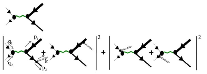
Figure 11: Diagrams for the calculation of the process (3).

From upper and lower diagrams of the Fig. 11 we have

$$\tilde{\Pi}_{2\to 2}=$$

$$d_{W}^{\alpha\beta}(q)d_{W}^{\alpha^{\prime}\beta^{\prime}}(q)\mathcal{F}^{(0)}_{\alpha\alpha^{\prime}}(-q_{1},0,-q_{2},0)\mathcal{F}^{(0)}_{\beta\beta^{\prime}}(p_{1},m_{t},p_{2},0),$$ (83)

$$I_{2}=\frac{6\sqrt{D_{12}(Q^{2},m_{t\;\perp},P_{t})}}{\pi}\frac{1-x_{m}^{2}}{(1-x_{w}^{2})^{2}}\times$$

$$\hskip 8.5359pt\left(3+C^{\prime 2}+(3-C^{\prime 2})x_{m}^{2}\right),$$ (84)

$$C^{\prime 2}=D_{12}(Q^{2},m_{t\;\perp},P_{t})/D_{12}(Q,m_{t},0),$$ (85)

$$x_{w}=m_{W}/Q,$$

and

$$\tilde{\Pi}_{2\to 3}=\biggl{\{}d_{W}^{\alpha\beta}(q)d_{W}^{\alpha^{\prime}\beta^{\prime}}(q)\mathcal{F}^{(0)}_{\alpha\alpha^{\prime}}(-q_{1},0,-q_{2},0)\times$$

$$\phantom{\tilde{\Pi}_{2\to 3}=\biggl{\{}}\tilde{\mathcal{F}}^{(1)}_{\beta\beta^{\prime}}(p_{1},m_{t},p_{2},0,k,K)+$$

$$\phantom{\tilde{\Pi}_{2\to 3}=\biggl{\{}}d_{W}^{\alpha\beta}(q-k)d_{W}^{\alpha^{\prime}\beta^{\prime}}(q-k)\mathcal{F}^{(0)}_{\beta\beta^{\prime}}(p_{1},m_{t},p_{2},0)\times$$

$$\phantom{\tilde{\Pi}_{2\to 3}=\biggl{\{}}\tilde{\mathcal{F}}^{(1)}_{\alpha\alpha^{\prime}}(-q_{1},0,-q_{2},0,k,K)\biggr{\}}$$ (86)

correspondingly, where

$$d^{\alpha\beta}_{W}(q)=\tilde{d}^{\alpha\beta}_{W}(q)/(q^{2}-m_{W}^{2}),\;\tilde{d}^{\alpha\beta}_{W}(q)=-g^{\alpha\beta}+\frac{q^{\alpha}q^{\beta}}{q^{2}},$$

and for all the calculations we put $m_{b}=0$ since$m_{b}/m_{t}\ll 1$.

For the process (4) and calculation of $N^{g}_{tq^{\prime}}$ we have the following functions (see diagrams on the Fig. 12)

$$\tilde{\Pi}_{2\to 2} \!= \!d_{W}^{\alpha\beta}(q_{1}-p_{1})d_{W}^{\alpha^{\prime}\beta^{\prime}}(q_{1}-p_{1})\times$$ (87)

$$\mathcal{F}^{(0)}_{\alpha\alpha^{\prime}}(p_{2},0,-q_{2},0)\mathcal{F}^{(0)}_{\beta\beta^{\prime}}(p_{1},m_{t},-q_{1},0),$$

$$I_{2} \!= \!\frac{288\sqrt{D_{12}(Q^{2},m_{t\;\perp},P_{t})}}{\pi}\times$$ (88)

$$\frac{1-x_{m}^{2}}{(1-x_{m}^{2}+2x_{w}^{2})^{2}-C^{\prime 2}(1-x_{m}^{2})^{2}},$$

where $C^{\prime}$ is the same as in the previous process.

$$\tilde{\Pi}_{2\to 3}=$$

$$\phantom{\tilde{\Pi}_{2\to 3}}\!\!\biggl{\{}d_{W}^{\alpha\beta}(q_{2}-p_{2})d_{W}^{\alpha^{\prime}\beta^{\prime}}(q_{2}-p_{2})\times$$

$$\phantom{\tilde{\Pi}_{2\to 3}}\!\!\mathcal{F}^{(0)}_{\alpha\alpha^{\prime}}(p_{2},0,-q_{2},0)\tilde{\mathcal{F}}^{(1)}_{\beta\beta^{\prime}}(p_{1},m_{t},-q_{1},0,k,K)+$$

$$\phantom{\tilde{\Pi}_{2\to 3}}\!\!d_{W}^{\alpha\beta}(q_{1}-p_{1})d_{W}^{\alpha^{\prime}\beta^{\prime}}(q_{1}-p_{1})\times$$

$$\phantom{\tilde{\Pi}_{2\to 3}}\!\!\mathcal{F}^{(0)}_{\beta\beta^{\prime}}(p_{1},m_{t},-q_{1},0)\tilde{\mathcal{F}}^{(1)}_{\alpha\alpha^{\prime}}(p_{2},0,-q_{2},0,k,K)\biggr{\}},$$ (89)

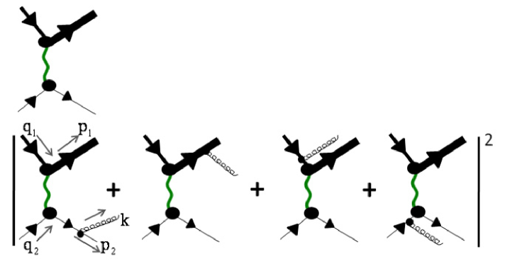
Figure 12: Diagrams for the calculation of the process (4).

Calculations for the process (5) and $N^{g}_{tW}$ looks as follows (see diagrams on the Fig. 10)

$$\tilde{\Pi}_{2\to 2} \!= \!\left.\tilde{d}_{W}^{\alpha\alpha^{\prime}}(p_{2})\right|_{p_{2}^{2}=m_{W}^{2}}\left.\tilde{d}^{\rho\rho^{\prime}}(q_{1},n)\right|_{n=\Delta}\times$$ (90)

$$\mathcal{F}^{(1)}_{\alpha\alpha^{\prime}\;\rho\rho^{\prime}}(p_{1},m_{t},-q_{2},0,-q_{1},0),$$

$$I_{2}=\!\frac{1}{\pi}\Biggl{\{}-2\sqrt{D_{12}(Q^{2},m_{t\;\perp},m_{W\;\perp})}\times$$

$$\biggl{[}u^{2}\left(1-C^{\prime 2}\right)+2x_{m}^{2}u^{2}\left(1+C^{\prime 2}-u^{2}\left(1-C^{\prime 2}\right)\right)+$$

$$x_{m}^{4}u^{2}\left(1-u^{2}\right)^{2}\left(1-C^{\prime 2}\right)\biggr{]}^{-1}\times$$

$$\biggl{[}\left(3-2u^{2}\right)\left(1-C^{\prime 2}\right)+$$

$$x_{m}^{2}\biggl{(}3\left(C^{\prime 2}+3\right)-u^{2}\left(C^{\prime 2}+7\right)-2u^{4}\left(1-C^{\prime 2}\right)\biggr{)}+$$

$$x_{m}^{4}\left(1-u^{2}\right)\biggl{(}25+3C^{\prime 2}+$$

$$u^{2}\left(23C^{\prime 2}+33\right)-10u^{4}\left(1-C^{\prime 2}\right)\biggr{)}+$$

$$3x_{m}^{6}\left(1+2u^{2}\right)\left(1-u^{2}\right)^{3}\left(1-C^{\prime 2}\right)\biggr{]}+$$

$$\frac{4(1+2u^{2})(1+2x_{m}^{2}(1-u^{2})+2x_{m}^{4}(1-u^{2})^{2})}{u^{2}}\times$$

$$\ln\frac{1+x_{m}^{2}(1-u^{2})+\sqrt{D_{12}(Q^{2},m_{t\;\perp},m_{W\;\perp})}}{1+x_{m}^{2}(1-u^{2})-\sqrt{D_{12}(Q^{2},m_{t\;\perp},m_{W\;\perp})}}\Biggr{\}},$$ (91)

where

$$C^{\prime 2} \!= \!D_{12}(Q^{2},m_{t\;\perp},m_{W\;\perp})/D_{12}(Q^{2},m_{t},m_{W}),$$

$$u \!= \!m_{W}/m_{t},$$ (92)

$$\tilde{\Pi}_{2\to 3} \!= \!\left(-g^{\mu\mu^{\prime}}+\frac{k^{\mu}k^{\mu^{\prime}}}{K^{2}}\right)\times$$ (93)

$$\left.\tilde{d}_{W}^{\alpha\alpha^{\prime}}(p_{2})\right|_{p_{2}^{2}=m_{W}^{2}}\left.\tilde{d}^{\rho\rho^{\prime}}(q_{1},n)\right|_{n=\Delta}\times$$

$$\mathcal{F}^{(2)}_{\alpha\alpha^{\prime}\;\mu\mu^{\prime}\;\rho\rho^{\prime}}(p_{1},m_{t},q_{1},0,q_{2},0,k,K).$$

References

(1) http://pdg.lbl.gov/
(2) D. Milstead, Phys.At. Nucl. 71, (2008) 618.
(3) A.V. Kisselev and V.A. Petrov, Phys.Part.Nucl. 39, (2008) 798.
(14) DELPHI Collab., J. Chrin et al., in Proc. of
the 27-th International Conference on High Energy Physics,
Glasgow, UK, 20-27 July 1994, eds. P.J. Bussey and I.G. Knowles,
p. 893.
(15) A. Bassetto, M. Ciafaloni, G. Marchesini, Phys. Rep. 100, (1983) 201.
(16) Yu.L. Dokshitzer, V.A. Khoze, A.H. Mueller, S.I. Troian, ”Basics of perturbative QCD”, Published in Gif-sur-Yvette, France: Ed. Frontieres (1991) 274 p.
(17) E. Leader, E.Predazzi, arXiv:1101.3425.
(18) OPAL Collab., G. Abbiendi et al., Phys. Lett. B 453, (1999) 153.
(19) DELPHI Collab., P. Abreu et al., Eur. Phys. J. C 18, (2000) 203.