Statistical mechanics of glass transition in lattice molecule models

Abstract

Lattice molecule models are proposed in order to study statistical mechanics of glass transition in finite dimensions. Molecules in the models are represented by hard Wang tiles and their density is controlled by a chemical potential. An infinite series of irregular ground states are constructed theoretically. By defining a glass order parameter as a collection of the overlap with each ground state, a thermodynamic transition to a glass phase is found in a stratified Wang tiles model on a cubic lattice.

1 Introduction

The equilibrium statistical mechanics successfully describes various types of phase transitions including ferromagnetic-paramagnetic transitions, gas-liquid transitions, and liquid-solid transitions. For structural glass transitions, whose precise definition is not obvious, the understanding has been accumulated from several viewpoints [1]. In particular, in addition to an insightful phenomenological argument [2, 3, 4, 5], which is often referred to as a random first-order transition scenario (RFOT), the analysis within the equilibrium statistical mechanics has provided quantitative results for structural glass transitions [6, 7, 8, 9, 10, 11]. At present, it has become widely conjectured that a thermodynamic glass transition, if it exists, is described as a one-step replica symmetry breaking (1RSB) in the spin glass terminology. Despite such successes, a theory of glass transition in finite-dimensional, short-range interaction systems is still one of challenging problems in physics, because the theory on the basis of equilibrium statistical mechanics has been established only for models with infinite-range interaction or on a random graph.

Here, let us recall a history of studies on critical phenomena. The van der Waals theory is the first breakthrough of theory for critical phenomena, which might correspond to RFOT for glass transitions. It should be noted that the statistical mechanics of a model with an infinite-range interaction exactly predicts critical phenomena in accordance with the van der Waals theory [12]. This reminds us a relation between 1RSB in mean-field type models and RFOT in phenomenology. Then, the existence of a critical point within the equilibrium statistical mechanics of short-range interaction Hamiltonians was shown by Peierls [13], Kramers-Wannier [14], and Onsager [15]. In particular, Onsager solved the two-dimension Ising model exactly and proved that critical phenomena in finite dimensions are qualitatively different from the van der Waals theory (or the Curie-Weiss theory in ferromagnetic-paramagnetic transitions). Since then, the significance of critical phenomena in finite dimensions has been recognized and much effort has been done in order to connect between Onsager’s result and the van der Waals theory. We now understand a great picture of critical phenomena.

However, with regard to glass transitions, there is no exactly solved example in finite dimensions; rather, there is no finite-dimensional, short-range interaction model for which the existence of a glass transition is understood theoretically. Thus far, toward establishment of statistical mechanics of glass transition in finite dimensions, several lattice models have been proposed. One example is a class of models proposed by Biroli and Mézard [8], in which at most $k$ neighboring particles are allowed to contact with each particle. Although this simple model exhibits a glass transition when it is defined on a random graph, crystallization occurs in finite-dimensional lattices except for subtle cases [16]. In the other model proposed by Ref. [17], crystallization might be prohibited, and the numerical experiment has been performed in order to explore the nature of thermodynamic glass transitions [18]. However, it seems difficult to develop a theoretical argument for this model in finite dimensions. Furthermore, finite-dimensional quenched-disordered spin models that exhibit 1RSB under the mean-field approximation have been studied numerically [19]. However, the numerical computation is much harder than standard spin glass models, and a precise theory for the model might be quite challenging. (See Ref. [20] as such a theoretical attempt.)

In contrast to previous studies, we first propose finite-dimensional hard-constraint models for which ground states can be constructed theoretically. Here, the ground states are obtained by taking the limit of the chemical potential to be infinitely large, because the chemical potential is the only thermodynamic intensive variable in such models. Indeed, we can show that our model possesses uncountably infinite number of ground states in the infinite size lattice, and typical ground states are irregular in the sense that they do not exhibit any long-range positional order characterized by the existence of Bragg peaks. Note that quasi-periodic ground states are classified as regular ground states. Let us denote a set of all ground-state configurations by ${\cal D}$, which we can specify theoretically for our models. Now, we introduce an overlap with a ground state configuration $\alpha\in{\cal D}$, which is denoted by $q_{\alpha}$. Since $q_{\alpha}$ is defined for each ground state $\alpha$, we have an infinite-dimensional vector ${\boldsymbol{q}}=(q_{\alpha})_{\alpha\in{\cal D}}$. We refer this vector to as the order parameter, because this corresponds to the magnetization in the Ising model.

We explain the correspondence by reviewing the phase transition in the two-dimensional Ising model. When the temperature is higher than the critical temperature, in the thermodynamic limit, there exists a unique expectation value of observables with being independent of boundary conditions. However, the independence of boundary conditions is broken below the critical temperature. In general, a state of the system without the uniqueness is referred to as the ordered phase. The dependence on boundary conditions is most easily observed when the expectation of the magnetization is considered under the spin-up boundary condition or the spin-down boundary condition. We here notice that the magnetization is equivalent to the overlap with one ground state. We thus consider the overlap with each ground state as the generalization of the magnetization. We also generalize spin-up and spin-down boundary conditions to special boundary conditions that uniquely determine a ground-state configuration for a series of system sizes going to the infinity. We call such a boundary condition a GS-boundary condition.

Since we have the glass order parameter ${\boldsymbol{q}}$ in our models, we can investigate whether or not the expectation value of ${\boldsymbol{q}}$ takes a different value under every GS-boundary condition. If the dependence is shown, the existence of an ordered phase characterized by the parameter ${\boldsymbol{q}}$ is claimed. From a fact that a typical ground state does not exhibit a long-range positional order, we identify the ordered phase as the glass phase. As far as we know, such an approach to glass problems has never been attempted.

This paper is organized as follows. In section 2, we start with a definition of lattice molecule models we study. The molecules in the models are represented by hard Wang tiles [21] and the molecule density obeys a grand canonical ensemble. In section 3, we consider a simple model in this class. We show that the model possesses an infinite series of irregular ground-states, while no thermodynamic transition occur. In section 4, as an extension of the model, we propose a three-dimensional model in which a thermodynamic glass transition is observed. We present theoretical arguments and numerical evidences for the thermodynamic glass transition. Section 5 is devoted to concluding remarks.

2 Lattice molecule model

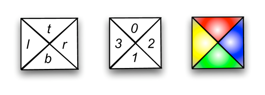
Figure 1: Unit square tile with colored edges.

Let $\Lambda_{L}=\{(i,j)\in{\bf N}\times{\bf N}|1\leq i,j\leq L\}$ be a square lattice. We formulate a statistical mechanical model in the lattice $\Lambda_{L}$. Each site can be occupied by at most one molecule. A molecule is characterized by its shape, represented by $m$-colors given on edges of a unit square. Since tiles with colored edges are called Wang tiles, the molecules in our model may be interpreted as Wang tiles.

When left, right, bottom and top edges of a Wang tile are colored by $\ell$, $r$, $b$ and $t$, respectively, we denote the quartet of colors by $(\ell,r,b,t)$. Below, the colors will be identified with integers if the correspondence is explicitly given. (See figure 1.) Among $m^{4}$ different Wang tiles, we select $p$ different tiles. These are called prototiles and the set of prototiles is denoted by $C$. Each prototile is represented by an integer $n$, $1\leq n\leq p$. At each site $x\in\Lambda_{L}$, we define $\sigma(x)=n$ if there is a molecule congruent to a prototile $n\in C$ and as $\sigma(x)=0$ if the site is empty. We call an empty site a hole. The set of tile configurations $(C\cup\{0\})^{\Lambda_{L}}$ is denoted by $\Sigma_{L}$. We study statistical mechanics of the molecules under a boundary condition imposed at sites in $\partial\Lambda_{L}^{-}$ and $\partial\Lambda_{L}^{+}$, where $\partial\Lambda_{L}^{-}\equiv\{(i,j)\in\Lambda_{L}|i=1\ {\rm or}\ j=1\}$ and $\partial\Lambda_{L}^{+}\equiv\{(i,j)\in\Lambda_{L}|i=L\ {\rm or}\ j=L\}$. The bulk region $\Lambda_{L}\backslash(\partial\Lambda_{L}^{+}\cup\partial\Lambda_{L}^{-})$ is denoted by $\bar{\Lambda}_{L}$, and the number of sites in the bulk region is $N=(L-2)^{2}$.

Specifically, we consider the case that the interaction between molecules is described by a hard constraint that molecules are allowed to contact each other only when contiguous edges of tiles have the same color. We then assume a grand canonical ensemble

$$P_{\mu}(\sigma)=\frac{1}{\Xi(\mu)}D(\sigma)e^{\mu N\rho(\sigma)},$$ (1)

where $D(\sigma)=1$ for configurations that satisfy the constraint that contiguous edges have the same color, otherwise $D(\sigma)=0$; $\mu$ is the chemical potential of molecules taking a value in $[-\infty,\infty]$, and $\rho(\sigma)$ is the density of molecules defined by

$$\rho(\sigma)=\frac{1}{N}\sum_{x\in\bar{\Lambda}_{L}}[1-\delta(\sigma(x),0)].$$ (2)

Here, the temperature is set to be unity and its value is irrelevant for the problem. The normalization constant $\Xi(\mu)$ in (1) is the partition function, which is explicitly given by

$$\Xi(\mu)=\sum_{\sigma\in\Sigma_{L}}D(\sigma)e^{\mu N\rho(\sigma)}.$$ (3)

Configurations realized in the limit $\mu\to\infty$ are ground-states in statistical mechanics. A tile configuration without holes, which is referred to as a complete tiling in this paper, provides a ground state.

Thermodynamic properties associated with the density are determined by the pressure function $p(\mu)$ defined by

$$p(\mu)\equiv\lim_{N\to\infty}\frac{1}{N}\log\Xi(\mu).$$ (4)

The expectation value of the density $\langle\rho\rangle$ is given by

$$\langle\rho\rangle=\frac{dp(\mu)}{d\mu}.$$ (5)

Furthermore, the entropy density $s$ is related to the pressure in term of the Legendre transformation

$$s(\rho)=\inf_{\mu}[p(\mu)-\rho\mu].$$ (6)

Statistical behavior of the model depends on the choice of a set of $p$-types of molecules $C$. As the simplest example, let us consider the set $C$ with $p=2$, in which all the edges of one type are red and all the edges of the other type are green. In this model, ground states are understood as the complete tilings occupied by one color when the open boundary condition $\sigma(x)=0$ for $x\in\partial\Lambda_{L}^{-}\cup\partial\Lambda_{L}^{+}$ is assumed. When $\mu$ is sufficiently large, the number density of red tiles depends on boundary condition even in the limit $L\to\infty$. On the other hand, when $\mu$ is sufficiently small (negatively large), tile configurations are disordered and all statistical quantities are independent of boundary conditions in the limit $L\to\infty$. The ${\bf Z}_{2}$ symmetry breaking occurs at some $\mu$ beyond which there exists an ordered phase. The universality class near the transition is identical to that of the two-dimensional Ising model.

A unique feature of Wang-tiles is that the operation of any Turing machine is simulated by a complete tiling for an appropriate set $C$. (See Ref. [21] for the research history. See also Ref. [22] as an instructive paper for this issue.) According to computation theory, this means that there is no algorithm that determines whether or not a complete tiling is possible for a given set $C$ [23]. In solving the decidability problem, it was a crucial step to find an aperiodic set of prototiles $C$ for which an aperiodic complete tiling in $\Lambda_{\infty}$ exists, while periodic complete tilings cannot be realized. After the first discovery, $p$, the number of elements of an aperiodic set has been reduced. At present, the minimum number of $p$ is 13 [24]. Statistical mechanics of a system consisting of an aperiodic set of 16-prototiles was studied in Ref. [25], where holes are not considered, but a positive energy is assumed for mismatches of contiguous colors. This reference claims that a thermodynamic transition occurs at some finite temperature. See also Ref. [26] for the recent study on the model.

Here, from a viewpoint of statistical mechanics, it is important to recognize that there exits a set $C$ with which non-trivial ground states can be obtained as complete tilings corresponding to computational processes. We do not need to stick to aperiodic sets of Wang tiles. More important thing in the context of glass problems is that ground states should not possess any long-range positional order. However, in the construction of complete tilings with using the aperiodic sets with $p=13$ and $p=14$ [27], the quasi-periodic maps are employed to yield the tiling [28], and therefore their complete tilings possess the quasi-periodic order. The construction method in the other cases are entirely different from the cases that $p=13$ and $14$, but at least for known examples in Ref. [21], the complete tilings seem to exhibit a long-range positional (quasi-periodic) order.

Now, let us recall a dynamical-system theory, which tells us that aperiodic motion described as a solution of a deterministic equation is further classified into quasi-periodic motion and irregular motion [29, 30]. Periodic and quasi-periodic motion are called regular motion and characterized by the existence of the singular peak in its spectrum. Then, there are an infinitely number of periodic orbits in typical chaotic systems and the exclusion of periodic orbits can be realized by systems that exhibit quasi-periodic motion. Similarly, it is reasonable to classify aperiodic configurations generated by a deterministic rule into quasi-periodic and irregular configurations. Quasi-periodic configurations are characterized by the existence of a singular peak in the Fourier transform (Bragg peak) of some representation of configuration, as is known in quasi-crystals [31]. See also Ref. [32] for a mathematical argument of the definition of weak crystals which cover certain generalization of quasi-crystals. In our viewpoint, non-periodic long-range positional order in Thue-Morse sequences [33] is classified into the same group as quasi-periodic order. Here, it should be noted that irregular configurations without any Bragg peaks can also be generated by a deterministic rule. In order to seek for thermodynamic glass transitions, we study statistical mechanics associated with such irregular (no periodic and no quasi-periodic) complete tilings in $\Lambda_{\infty}$.

From this reason, we are not concerned with aperiodic sets of prototiles, but with the case that complete tilings are irregular almost surely when a complete tiling is picked up with the equal weight, while there exists a countably infinite number of periodic complete tilings. We shall provide an example in the next section.

3 4-prototiles model

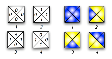
Figure 2: Set of 4-prototiles. The left figure shows a number representation. The tiles satisfy $t=r=\ell+b$ (mod 2). The right figure shows a color representation.

The simplest set of Wang prototiles that generates irregular complete tilings is given in figure 2. This set is characterized by a rule that the quartet $(\ell,r,b,t)$ satisfies $t=r=\ell+b$ (mod 2), where $r$, $\ell$, $b$ and $t$ are either 0 or 1. For this model, we shall show that (i) there are an uncountably infinite number of irregular complete tilings, but (ii) no thermodynamic transition occurs.

3.1 Complete tilings

2 3	1	3	4
1 4	0	1	2
		0	1
		1 4	2 3

Table 1: Cellular automaton rule for generating complete tilings in $\Lambda_{\infty}$. When $r$ of the left tile and $t$ of the bottom tile are given, the tile is uniquely determined. The rule is equivalent to Rule 102 in Ref. [34].

Complete tilings in this model are obtained as follows. For an element $([h(i)]_{i=1}^{L},[v(j)]_{j=1}^{L})$ in the set ${\cal D}_{L}\equiv\{0,1\}^{L}\times\{0,1\}^{L}$, we set $\ell(1,j)=v(j)$ and $b(i,1)=h(i)$. Then, by the rule in table 1, tiles at $(i,1)$, $2\leq i\leq L$, are determined from smaller $i$ in order. Similarly, the tiles at $(i,j)$, $1\leq i\leq L$, are determined for $j=2,3,\cdots,L$. In this manner, all the complete tilings in $\Lambda_{L}$ are uniquely coded by ${\cal D}_{L}$. That is, there are $2^{2L}$ complete tilings for the system of size $L$. The complete tilings in $\Lambda_{\infty}$ are obtained in the limit $L\to\infty$. Since ${\cal D}_{\infty}$ has one-to-one correspondence with real numbers in the interval $[0,1]$, the cardinality of the complete tilings in $\Lambda_{\infty}$ are uncountably infinite. Since periodic tilings are countable, almost all complete tilings are aperiodic.

A remarkable feature of the complete tilings is the additivity. Suppose that $\sigma_{1}$ and $\sigma_{2}$ are different complete tilings, respectively. Here, we define the addition of two configurations $\sigma_{1}$ and $\sigma_{2}$ by determining $\ell(x)$ and $b(x)$ as

$$\ell(x) = \ell_{1}(x)+\ell_{2}(x)\quad({\rm mod}\quad 2),$$ (7)

$$b(x) = b_{1}(x)+b_{2}(x)\quad({\rm mod}\quad 2)$$ (8)

at each site $x\in\Lambda_{L}$. We denote this addition by $\sigma_{1}\oplus\sigma_{2}$. Then, from the coloring rule in figure 2, we find that the configuration $\sigma_{1}\oplus\sigma_{2}$ is also another complete tiling. Note that the configuration $\sigma(x)=1$ for all $x\in\Lambda_{L}$ is one of complete tilings. This tiling, which is denoted by $\sigma_{0,0}$, is the unit element in the additive group consisting of all complete tilings. As the simplest complete tiling other than $\sigma_{0,0}$, we generate a configuration from a condition that $h(i_{0})=1$ and $h(i)=0$ for $i\not=i_{0}$ and $v(j)=0$ for any $j$. As displayed in the left-side of figure 3, a fractal pattern, which is known as a Sierpinski gasket, is obtained. We denoted it by $\sigma_{i_{0},0}$. Similarly, we can generate a fractal configuration $\sigma_{0,j_{0}}$ from $v(j_{0})=1$ and $v(j)=0$ for $j\not=j_{0}$ and $h(i)=0$ for any $i$. All complete tilings in $\Lambda_{\infty}$ are given by a superposition of these basic configurations as

$$\sum_{i,n=1}^{\infty}\bigcirc\hskip 5.0pt[h(i)\sigma_{i,0}\oplus v(j)\sigma_{0,j}],$$ (9)

where $\sum\circ\hskip 5.0pt$ represents the summation of the configurations in the sense of $\oplus$. When we uniformly choose one complete tiling, it is given by a random superposition of Sierpinski gaskets, as displayed in the right side of figure 3. The randomness of $h(i)$ and $v(j)$ in (9) yields irregular configurations.

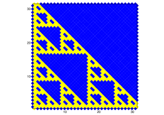
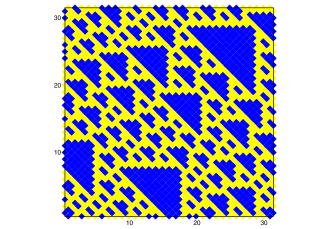
Figure 3: Examples of complete tilings. $L=32$. Left: $h(i)=\delta(i,1)$ and $v(j)=0$. Right: $h(i)$ and $v(j)$ are chosen randomly.

As a preliminary for later arguments, we define the overlap ratio between two complete tilings $\alpha,\alpha^{\prime}\in{\cal D}_{\infty}$:

$$q_{\alpha,\alpha^{\prime}}\equiv\frac{1}{L^{2}}\sum_{x\in\Lambda_{L}}\delta(\sigma_{\alpha}(x),\sigma_{\alpha}(x)),$$ (10)

and we consider the probability density $P_{\rm GS}(q)$ that $q_{\alpha,\alpha^{\prime}}$ takes a value $q$ when $\alpha$ and $\alpha^{\prime}$ are sampled uniformly. Since the 4-prototiles in our model are distributed with an equal ratio for a typical sample uniformly chosen from ${\cal D}_{\infty}$, we have $P_{\rm GS}(q)=\delta(q-1/4)$ in the limit $L\to\infty$.

At the end of section 3.1, let us remark previous studies related to the 4-prototiles model. The complete tilings of the model are essentially the same as the ground-state configurations of a three-body interaction spin model defined on upward triangles [35, 36, 37]. While an extremely slow dynamics is observed, no thermodynamic phase transition occur at a finite temperature. Recently, it has been shown that the system under a magnetic field, which is equivalent to a lattice gas model with a chemical potential, exhibits a first-order transition in the $(T,\mu)$ space [38]. Although non-trivial nature of the coexistence phase has been conjectured, further studies remain to be done.

3.2 Statistical Mechanics

We consider statistical mechanics of the 4-prototiles model. It is convenient to introduce a hole variable

$$\eta(x)\equiv\delta(\sigma(x),0).$$ (11)

That is, $\eta(x)=1$ only if the site $x$ is empty. For a given hole configuration $\eta\in\{0,1\}^{N}$, we define a region $N_{\eta}\equiv\{x\in\Lambda_{L}|\eta(x)=0\}$ in which tiles occupy the sites. Let $\tilde{\sigma}:N_{\eta}\to C$ be a restriction of $\sigma$ on the region $N_{\eta}$. Any configuration $\sigma$ can be then expressed by variables $\eta$ and $\tilde{\sigma}$. The partition function $\Xi(\mu)$ is expressed as

$$\Xi(\mu)=\rme^{\mu N}\sum_{\eta\in\{0,1\}^{N}}\rme^{-\mu\sum_{x\in\bar{\Lambda}_{L}}\eta(x)}\Omega(\eta),$$ (12)

where $\Omega(\eta)$ is the number of possible tile configurations $\tilde{\sigma}$ when a hole configuration $\eta$ is given. We here fix one complete tiling $\alpha$ in $\Lambda_{\infty}$. We assume a boundary condition that $\sigma(x)=\sigma_{\alpha}(x)$ for $x\in\Lambda_{L}^{-}$ and $\sigma(x)=0$ for $x\in\Lambda_{L}^{+}$. We can calculate $\Omega(\eta)$ most easily under the boundary condition. Note that the pressure function $p(\mu)$ in the thermodynamic limit does not depend on the choice of boundary conditions.

The number $\Omega(\eta)$ is estimated as follows. It is obvious that $\Omega(\eta)=1$ when there are no holes. Suppose that there is a hole at the site $(i_{1},n_{1})$. Then, two tiles are possible at the site $(i_{1}+1,n_{1})$ if there is no hole at the site $(i_{1}+1,n_{1})$. We choose one tile of the two. For each choice, another tile configuration is uniquely determined by repeating the rule in Table 1 with starting from the site $(i_{1}+1,n_{1})$. Note that the configurations are consistent with the boundary conditions at $i=L$ and $n=L$. Similarly, there are two tile configurations that originate from the tile replaced at the site $(i_{1},n_{1}+1)$ if there is no hole at the site $(i_{1},n_{1}+1)$. Therefore, the number of possible configurations is

$$2^{1-\eta(i_{1}+1,n_{1})}\cdot 2^{1-\eta(i_{1},n_{1}+1)},$$ (13)

where we set $\eta(L,n)=\eta(i,L)=1$ in accordance with the boundary conditions.

Next, we assume that there is another hole at the site $(i_{2},n_{2})$. Then, in a manner similar to the first case, the number of possible tile configurations is assigned to this hole. The important thing here is that this estimation is obtained with being independent of configurations generated from the first hole at the site $(i_{1},n_{1})$. Since there is no over-counting of configurations, the number of possible configurations is

$$2^{1-\eta(i_{1}+1,n_{1})}\cdot 2^{1-\eta(i_{1},n_{1}+1)}\cdot 2^{1-\eta(i_{2}+1,n_{2})}\cdot 2^{1-\eta(i_{2},n_{2}+1)}.$$ (14)

Repeating these considerations for all holes, we arrive at the expression

$$\Omega(\eta)=\prod_{i,n}2^{\eta(i,n)(1-\eta(i+1,n))}2^{\eta(i,n)(1-\eta(i,n+1))}.$$ (15)

By introducing a spin variable $s(x)\equiv 2\eta(x)-1$, we rewrite (15) as

$$\Omega(\eta)=e^{\frac{J}{2}N-H(s)},$$ (16)

with a Hamiltonian

$$H(s)=\frac{J}{4}\sum_{\langle x,x^{\prime}\rangle}s(x)s(x^{\prime}),$$ (17)

where $J=\log(2)$ and $\langle x,x^{\prime}\rangle$ represents a nearest neighbor pair $x$ and $x^{\prime}$. Therefore, the partition function given in (12) is expressed as

$$\Xi(\mu)=\rme^{\frac{\mu}{2}N+\frac{J}{2}N}\sum_{s\in\{-1,1\}^{N}}\rme^{-H(s)-\frac{\mu}{2}\sum_{x}s(x)}.$$ (18)

That is, $\Xi(\mu)$ is determined from the canonical partition function for the anti-ferromagnetic Ising model under a magnetic field. Since $J/4=0.173..$ is less than the critical point $\beta_{\rm c}\simeq 0.44...$ of the Ising model, the pressure function $p(\mu)$ does not exhibit any singularities as a function of $\mu$. Thus, there is no thermodynamic transition in this model. Related with the problem, we remark that the expression (18) with (17) suggests the existence of a phase transition if $J$ were larger than $4\beta_{\rm c}$. Such a case may arise in a $p$-prototiles model with sufficiently large $p$. The transition in this case is regarded as an entropy-driven crystallization of holes. Although it is an interesting phenomenon, we do not discuss it in this paper.

Let us recall that there are an infinite series of complete tilings. When $\mu\to\infty$ is considered for fixed $L$, the expectation value of some observables depends on the boundary conditions in the infinite size limit. Note that this limit is different from the case $\mu\to\infty$ in the infinite system in which $L\to\infty$ is considered for the system with $\mu<\infty$. Since there is no thermodynamic transition, no boundary condition dependence of quantities is observed in the latter case. That is, once holes are generated in a complete tiling with any positive ratio, the system becomes free from boundary conditions despite the infinite degeneracy of complete tilings. We may say that complete tilings in the infinite system are unstable with respect to generation of holes. The origin of the instability is understood from the fact that an infinite region is influenced as the result of iteration of the cellular-automaton rule from one hole. (Recall the argument above (13).) Although a cellular-automaton rule can easily generate an infinite series of irregular complete tilings, it simultaneously leads to the instability of complete tilings so that a thermodynamic transition is not observed. In order to have stable complete tilings against generation of holes, we need to avoid a chain of tile-replacements induced by one hole.

4 Stratified Wang tiles

Let $\Lambda_{L,M}\equiv\{(i,j,k)\in{\bf N}\times{\bf N}\times{\bf N}|1\leq i,j\leq L,1\leq k\leq M\}$ be a cubic lattice. As a natural extension of the models in the previous section, we consider stratified Wang tiles in $\Lambda_{L,M}$. In addition to the color matching condition in each $(i,j)$ plane with $k$ fixed, we further impose a constraint condition that two neighboring prototiles in the $k$ direction, if they exists, are the same type. We define $\sigma(x)=n$ if there is a molecule congruent to a prototile $n\in C$ on the site $x\in\Lambda_{L,M}$ and as $\sigma(x)=0$ if the site $x$ is empty. Specifically, we consider the 4-prototype model studied in the previous section. A complete tiling in this model is given by $\sigma(i,j,k)=\sigma_{\alpha}(i,j)$ for $\alpha\in{\cal D}_{\infty}$. We denote it by $\sigma_{\alpha}(x)$ for $x\in\Lambda_{L,M}$.

We study statistical mechanics of the model with a boundary condition imposed at sites in $\partial\Lambda_{L,M}^{-}$, $\partial\Lambda_{L,M}^{+}$, and $\partial\Lambda_{L,M}^{\rm vert}$. where $\partial\Lambda_{L,M}^{-}\equiv\{(i,j,k)\in\Lambda_{L,M}|i=1\ {\rm or}\ j=1\}$, $\partial\Lambda_{L,M}^{+}\equiv\{(i,j,k)\in\Lambda_{L,M}|i=L\ {\rm or}\ j=L\}$, and $\partial\Lambda_{L,M}^{\rm vert}\equiv\{(i,j,k)\in\Lambda_{L,M}|k=1\ {\rm or}\ k=M\}$. The number of sites in the bulk region is $N=(L-2)^{2}(M-2)$. Without confusion, the notations in the two-dimensional case are also employed in the stratified model. We assume that $\sigma$ obeys the grand canonical ensemble

$$P_{\mu}(\sigma)=\frac{1}{\Xi(\mu)}D(\sigma)e^{\mu N\rho(\sigma)},$$ (19)

where $D(\sigma)=1$ for configurations that satisfy the constraints that contiguous edges of tiles in the $(i,j)$ plane for each $k$ have the same color and that neighboring prototypes in the $k$ direction are the same type, otherwise $D(\sigma)=0$; $\mu$ is the chemical potential of molecules, and $\rho(\sigma)$ is the density of molecules defined by

$$\rho(\sigma)=\frac{1}{N}\sum_{x\in\bar{\Lambda}_{L,M}}[1-\delta(\sigma(x),0)].$$ (20)

The normalization constant $\Xi(\mu)$ in (19) is the partition function of the stratified model.

4.1 Glass transition

We explain the existence of a thermodynamic transition in this model. We fix a complete tiling $\alpha\in{\cal D}_{\infty}$. We study statistical mechanics (19) of the system by assuming a boundary condition that

$$\sigma(x)=\sigma_{\alpha}(x)$$ (21)

for $x\in\partial\Lambda_{L}^{-}$ and $\sigma(x)=0$ for the other boundary sites. We refer it to as a GS-boundary condition, because the ground-state configuration is uniquely determined by this condition. The expectation value under the GS-boundary condition is denoted by $\langle\ \rangle_{\alpha}^{L,M}$. Here, let us recall that the up-spin boundary condition of the Ising model under which the ground state is uniquely determined despite the system possesses the up-down symmetry. The order parameter of the Ising model is the magnetization and it is interpreted as the overlap with the ground-state configuration. Similarly, in our model, as an order parameter associated with the complete tiling $\alpha$, we define an overlap variable with $\alpha$ as

$$q_{\alpha}(\sigma)\equiv\frac{1}{N}\sum_{x\in\bar{\Lambda}_{L,M}}\delta(\sigma(x),\sigma_{\alpha}(x)).$$ (22)

Now, we consider the case that $1\ll\rme^{\mu}\ll L=M$. A typical configuration in this case is given by a random deposition of holes with a probability with $e^{-\mu}+O(\rme^{-2\mu})$ for each site. When a hole is inserted to the complete tiling, no other tile configurations are allowed, which is different from the two-dimensional case discussed in the previous section. A tile different from $\sigma_{\alpha}$ at a site $x_{0}$ appears when four holes enclose the site $x_{0}$. The probability of such a configuration is $2\rme^{-4\mu}+O(\rme^{-5\mu})$. In general, we expect that $\lim_{L\to\infty}\langle q_{\alpha}\rangle_{\alpha}^{L,L}$ is expressed as a convergent expansion in $\rme^{-\mu}$ for sufficiently large $\mu$. That is,

$$\lim_{L\to\infty}\langle q_{\alpha}\rangle_{\alpha}^{L,L}=1-e^{-\mu}+O(e^{-2\mu}).$$ (23)

for large $\mu$. A more precise estimation on the basis of a Peierls argument should be presented. (See a brief discussion in section 5.)

Next, we assume the open boundary condition that $\sigma(x)=0$ for all the boundary sites. We denote the expectation value under the boundary condition by $\langle\ \rangle_{0}^{L,L}$. Then, when $\mu$ is sufficiently large, a typical configuration is close a complete tiling, but it is not identical to $q_{\alpha}$, in general. As discussed in section 3.1, the overlap ratio between two different complete tilings is $1/4$. We thus obtain

$$\lim_{L\to\infty}\langle q_{\alpha}\rangle_{0}^{L,L}\simeq\frac{1}{4}$$ (24)

for sufficiently large $\mu$. By comparing (23) and (24), we conclude that the expectation value of the observable $q_{\alpha}$ depends on boundary conditions in the infinite size limit. This means that there exists the ordered phase in the system with sufficiently large $\mu$. In the other limit where $\mu$ is sufficiently small (negatively large), statistical properties are independent of boundary conditions, because dilute tiles are almost non-interacting. Thus, there exists a thermodynamic transition at some value of $\mu$.

The quantity characterizing the ordered phase is a collection of $q_{\alpha}$, which is denoted by ${\boldsymbol{q}}=(q_{\alpha})_{\alpha\in{\cal D}_{\infty}}$. Formally, the order parameter ${\boldsymbol{q}}$ is an uncountably infinite dimensional vector. Such an order parameter is quite peculiar. To our best knowledge, no examples in finite dimensions have been reported. We also recall that a typical complete tiling $\alpha$ does not exhibit Bragg peaks in its Fourier transform. From these conditions, we identify the thermodynamic transition to the ordered phase with the glass transition to the glass phase characterized by ${\boldsymbol{q}}$.

4.2 Numerical experiments

We report results of numerical experiments for the stratified 4-prototiles model. In order to facilitate the equilibration, we employ the exchange Monte Carlo method [39]. We prepare $K$ replicas of the system with $\mu_{k}=\mu_{\rm max}k/K$, $k=1,\cdots,K$. In this paper, we set $\mu_{\rm max}=2$ and $K=40$. We estimate the expectation value $\langle A\rangle_{\alpha}^{L,M}$ for an observable $A(\sigma)$ by the time average of $A(\sigma(t))$ during the time interval $[t_{\rm w},2t_{\rm w}]$ with discarding the transient data $[0,t_{\rm w}]$, where the initial condition was assumed to be $\sigma=\sigma_{\alpha}$ for all $\mu_{k}$. When the time average of $A(\sigma(t))$ is independent of $t_{\rm w}$ within statistical errors, we assume that the result provides the estimation of equilibrium values $\langle A\rangle_{\alpha}^{L,M}$.

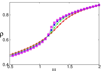
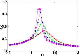
Figure 4: Statistical quantities of the density. $(L,M)=(12,8)$ (plus), $(15,10)$ (cross), $(18,12)$ (asterisk), and $(21,14)$ (box). Error-bars are within the symbols. Left: Expectation value of the density. Right: Fluctuation intensity of density $\chi$.

In the left side of figure 4, $\bar{\rho}\equiv\langle\rho\rangle_{\alpha}^{L,M}$ is plotted as a function of $\mu$ for the system with four different system sizes. In order to clarify the singular nature, the fluctuation intensity defined by $\chi\equiv N\langle(\rho-\bar{\rho})^{2}\rangle_{\alpha}^{L,M}$ is also displayed in the right side of figure 4. It should be noted that the fluctuation relation $\chi=d\bar{\rho}(\mu)/d\mu$ holds. The graphs of $\chi$ indicate the existence of a thermodynamic transition.

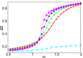
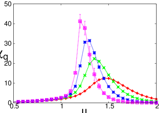
Figure 5: Statistical quantities of the glass order parameter. $(L,M)=(12,8)$ (plus), $(15,10)$ (cross), $(18,12)$ (asterisk), and $(21,14)$ (box). Error-bars are within the symbols expect for $\chi_{q}$ with $(L,M)=(21,14)$. Left: Expectation value $\langle q_{\alpha}\rangle_{\alpha}^{L,M}$ and $\langle q_{\alpha}\rangle_{0}^{12,8}$ (circle). Right: Fluctuation intensity of the order parameter $\chi_{q}$.

Next, we numerically investigate the existence of the glass phase by measuring the order parameter $q_{\alpha}$. In the left side of figure 5, we display $\bar{q}\equiv\langle q_{\alpha}\rangle_{\alpha}^{L,M}$ and $\langle q_{\alpha}\rangle_{0}^{L,M}$, which shows the boundary condition dependence of the expectation value of $q$. From the size dependence, we expect that the behavior sustains in the infinite size limit. This means that the transition is identified with the glass transition. Note that the expectation value of the density is independent of boundary conditions in the thermodynamic limit. In order to characterize the singularity associated with the order parameter, we measured $\chi_{q}\equiv N\langle(q_{\alpha}-\bar{q})^{2}\rangle_{\alpha}^{L,M}$. As shown in the right side of figure 5, $\chi_{q}$ exhibits a divergent behavior at some value of $\mu$.

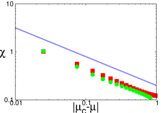
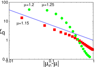
Figure 6: Left: Log-log plot of $\chi$ as a function of $|\mu_{\rm c}-\mu|$, where $\mu_{\rm c}$ is assumed to be $1.175$, for $(L,M)=(21,14)$. The square symbols correspond to the case $\mu<\mu_{\rm c}$ and the circle symbols to $\mu>\mu_{\rm c}$. The guide line represents $\chi=0.2|(\mu_{\rm c}-\mu)|^{-0.6}$. Right: Log-log plot of $\chi_{q}$ as a function of $|\mu_{\rm c}-\mu|$, where $\mu_{\rm c}$ is assumed to be $1.17$, for $(L,M)=(21,14)$. The square symbols correspond to the case $\mu<\mu_{\rm c}$ and the circle symbols to $\mu>\mu_{\rm c}$. The guide line represents $\chi_{q}=(\mu_{\rm c}-\mu)^{-0.8}$.

Here, we study the nature of the singularity quantitatively. We first attempt to fit the fluctuation intensities $\chi$ and $\chi_{q}$ with power-law functions as $|\mu-\mu_{\rm c}|$, where $\mu_{\rm c}$ is a transition point. As displayed in the left side of figure 6, $\chi$ may exhibit a power-law behavior

$$\chi\simeq|\mu-\mu_{\rm c}|^{-\alpha},$$ (25)

with $\alpha\simeq 0.6$ and $\mu_{\rm c}=1.175$. This result indicates that the transition is the second order according to the Ehrenfest classification. On the other hand, a clear power-law behavior is not observed in $\chi_{q}$. As shown in the right side of figure 6, a fitting of the power-law form $\chi_{q}\simeq(\mu_{\rm c}-\mu)^{-\gamma}$ might be not so bad with $\gamma\simeq 0.8$ when we choose a value of $\mu_{\rm c}$ ($\mu_{\rm c}=1.17$). However, $\chi_{q}$ in the regime $\mu>\mu_{\rm c}$ is far from power-law behaviors even if we change the value of $\mu_{\rm c}$. The singular nature of order parameter fluctuations is quite unusual.

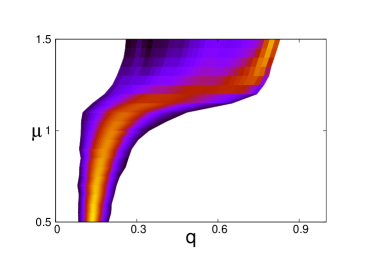
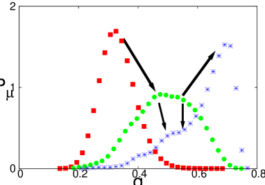
Figure 7: Left: Color representation of $P_{\mu}(q)$ in the $(q,\mu)$ space. $(L,M)=(21,14)$. Right: $P_{\mu}(q)$ with $\mu=1.15$ (square), $\mu=1.2$ (circle), and $1.25$ (asterisk). The error-bars are within the symbols.

In order to demonstrate the peculiar behavior more, we consider the distribution function of $q$ for the system with $\mu$, which is denoted by $P_{\mu}(q)$. The left side of figure 7 shows that the peak of $P_{\mu}(q)$ for $\mu>\mu_{\rm c}$ accompanies a broad tail in the smaller $q$ region. We investigate $P_{\mu}(q)$ near a transition point carefully in the right side of figure 7. Let us focus on the graph with $\mu=1.25$ represented by the asterisk symbols, which corresponds to the second left of circle symbols in the right of figure 6. There is a small slope regime around $q=0.5$ which is apart from the main peak $q=0.7$. The left edges of the regime seems to be connected to the left edge of the nearly flat regime of the graph with $\mu=1.2$, which corresponds to the most left of circle symbols in the right of figure 6. The left edge of the flat regime may be further connected to the main peak of the graph with $\mu=1.15$, which corresponds to the most left of square symbols in the right of figure 6. On the other hand, the main peak of the graph with $\mu=1.25$ arises from the right edge of the flat regime of the graph with $\mu=1.2$. The important thing here is that the main peak in the ordered phase is not connected to the main peak in the disordered phase. This suggests the discontinuous transition of $\langle q\rangle_{\alpha}^{L,M}$ in the thermodynamic limit $L,M\to\infty$, although a clear discontinuous jump is not observed in the left side of figure 5. Extensive numerical studies are necessary to have firm evidences for supporting the conjecture, because the sizes we investigated are too small. In any cases, we can say that the behavior of the order parameter ${\boldsymbol{q}}$ is quite unusual.

5 Concluding remarks

In this paper, we have proposed lattice molecule models, one of which exhibits the thermodynamic glass transition in three dimensions. The glass phase is characterized by the uncountably-infinite dimensional order parameter ${\boldsymbol{q}}$, each component of which measures the overlap with an irregular ground state. We conjecture that the transition is the second-order in the sense of thermodynamics, while the glass order parameter exhibits a unusual behavior. Before ending the paper, we describe problems that should be studied seriously in future.

Although we have studied the system with the simplest set of 4-prototiles that generates irregular complete tilings, statistical behavior of lattice molecule models depends on the choice of prototiles. By studying models with other sets of prototiles, we wish to classify their phenomena. In particular, it is interesting to find a two-dimensional model that exhibits a glass transition or to prove that there is no such a model. Note that the thermodynamic transition to the quasi-periodic ordered phase was observed in a two-dimensional Wang-tiles model [25, 26]. The difference between the quasi-periodic order and the glass order should be clarified. In doing these studies, extensive numerical experiments are necessary. It is significant to develop an efficient method for numerical calculation. The hard nature of molecules would substantially reduce the computation time if an elegant algorithm is found.

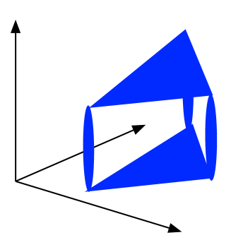
Figure 8: Schematic figure of a simple interface configuration with large $\eta$. Holes in the top and bottom triangles form Sierpinski gaskets and the vertexes of the triangles are connected by holes in the vertical directions.

Since the theoretical arguments reported in this paper are still in the early stage of the study, important theoretical problems remain to be solved. The first problem is to provide a mathematical proof of the existence of the glass transition. This might be solved as follows. We consider a probability that $\sigma$ at the center site $x_{0}$ is different from $\sigma_{\alpha}$ under the boundary condition $\sigma=\sigma_{\alpha}$ for all boundary sites. We estimate an upper-bound of the probability by noting an interface separating an ordered region connected to the boundary sites. (See an example of an interface in figure 8.) If this is explicitly defined for a given arbitrary configuration in which $\sigma(x_{0})\not=\sigma_{\alpha}(x_{0})$, we may formulate a Peierls argument. That is, a transition is understood from the competition between the entropy cost of configurations with interfaces and the energy cost of holes. However, up to the present, we do not have an explicit definition of such interfaces.

A more important but difficult problem is to obtain a mathematical description of statistical properties of the glass order parameter ${\boldsymbol{q}}$. When we consider this problem, it seems better to forget the tile model. Instead, we will analyze a stratified model of the 3-body spin interaction on upward triangles. (See a remark at the end of section 3.1.) By applying the same argument in the present paper to the spin model, we may find a glass transition for the stratified model. Since this model is much simpler than the tile model, several theoretical calculations including a sort of the Bethe approximation will be done more easily. Such theoretical study may provide a connection to the mean-field picture of the glass transition (RFOT). Furthermore, it is amazing if we find an exactly solved model that exhibits a glass transition. An exact solved model would play a crucial influence on the study of glass transitions.

In the analysis of infinite-range interaction models that exhibit a glass transition, the number of pure states in the glass phase has been one of concerns. With regard to this problem, we briefly review Gibbs measures of infinite-size systems. Roughly speaking, a Gibbs measure is defined in such a way that the probability of configurations in any finite-size region is given by the grand canonical ensemble with boundary conditions which are chosen by the measure. In the disordered phase, the Gibbs measure is unique, while there are an infinite number of Gibbs measures if the uniqueness is broken. In particular, a special measure that cannot be decomposed further into a superposition of other Gibbs measures is called a pure state. Here, let us recall that each GS-boundary condition in the Ising model can provide a pure state. Although GS-boundary conditions are not always related to pure states, the statistical ensembles in finite systems under GS-boundary conditions may be a starting point for understanding of pure states in the glass phase.

Finally, we go back to our motivation of understanding the nature of glassy materials. Although we have found a thermodynamic glass transition in a short-range interaction model in finite dimensions, it is not obvious whether or not such an idealized phase is actually observed in laboratory experiments. Toward an experimental realization of thermodynamic glass phases, we need to consider the following problems. The first is to construct a mechanical model that exhibits a glass transition. Although we have only to design a potential function sharing common features with hard-constraint conditions in Wang tiles, its explicit demonstration may be challenging. The second problem is to find an experimentally realizable algorithm for facilitating the equilibration, because the exchange MC method cannot be employed in laboratory experiments. After solving the problems, we hope that we will be able to demonstrate by numerical experiments that a genuine thermodynamic glass transition is observed in laboratories.

References

References

- [1] Cavagna A 2009 Physics Reports 476, 51
- [2] Gibbs J H and DiMarzio E A 1958 J. Chem. Phys. 28, 373
- [3] Adam G and Gibbs J H 1965 J. Chem. Phys. 43, 139
- [4] Kirkpatrick T R, Thirumalai D, and Wolynes P G, 1989 Phys. Rev. A 40, 1045
- [5] Bouchaud J P and Biroli G 2004 J. Chem. Phys. 121 7347
- [6] Monasson R 1995 Phys. Rev. Lett., 75, 2847
- [7] Mézard M and Parisi G 1999 Phys. Rev. Lett. 82 747
- [8] Biroli G and Mézard M 2002 Phys. Rev. Lett. 88, 025501
- [9] Rivoire O et al 2004 Eur. Phys. J. B 37, 55
- [10] Krzakala F, Tarzia M, Zdeborová L 2007 Phys. Rev. Lett. 101, 165702
- [11] Parisi G and Zamponi F 2010 Rev. Mod. Phys. 82 789
- [12] Gallavotti 1999 Statistical Mechanics A Short Treatise (Springer, Berlin)
- [13] Peierls R 1936 Proceesdings of Cambridge Philosphical Society 32 477
- [14] Kramers H A and Wannier G H 1941 Phys. Rev. 60 252
- [15] Onsager L 1944 Phys. Rev. 65 117
- [16] Hukushima K and Sasa S 2010 J. Phys.: Conf. Ser. 233 012004
- [17] Pica Ciamarra M, Tarzia M, de Candia A, and Coniglio A 2003 Phys. Rev. E. 67 057105
- [18] Parisi G 2009 arXiv:0911.2265
- [19] Brangian C, Kob W, and Binder K 2002 J. Phys. A: Math.Gen. 35 191
- [20] Moore M A 2006 Phys. Rev. Lett. 96 137202
- [21] Grünbaum B and Shephard G C 1987 Tilings and Patterns (W. H. Freeman and Company, New York)
- [22] Robinson R M 1971 Inventions Math. 12 177
- [23] Davis M 1982 Computability and Unsolvability (Dover, New York)
- [24] Culik II, K 1996 Discrete Mathematics 160 245
- [25] Leuzzi L and Parisi G 2000 J. Phys. A:Math. Gen. 33 4215
- [26] Aristoff D and Radin C 2011 arXiv:1102.1982
- [27] Kari J 1996 Discrete Mathematics 160 259
- [28] The author learned this fact from T. Chawanya.
- [29] Powell G E and Percival I C 1979 J. Phys. A: Math. Gen, 12 2053
- [30] Eckmann J P and Ruelle D 1985 Rev. Mod. Phys. 57 617
- [31] Janssen T 1988 Physics Report 168 55
- [32] van Enter A C D, Miekisz J 1992 J. Stat. Phys. 66 1147
- [33] van Enter A C D, Miekisz K, and Zahradnik M 1998 J. Stat. Phys. 90 1441
- [34] Wolfram S 1983 Rev. Mod. Phys. 55 601
- [35] Newman M E J and Moore C 1999 Phys. Rev. E 60 5068
- [36] Garrahan J P and Newman M E J 2000 Phys. Rev. E 62 7670
- [37] Jack R and Garrahan J P 2005 J. Chem. Phys 123 164508
- [38] Sasa S 2010 J. Phys. A: Math. Theor. 43 465002
- [39] Hukushima K and Nemoto K 1996 J. Phys. Soc. Jpn. 65 1604