Quantitative determination of the discretization and truncation errors in the numerical renormalization-group calculations of spectral functions

Abstract

In the numerical renormalization group (NRG) calculations of spectral functions of quantum impurity models, the results are always affected by discretization and truncation errors. The discretization errors can be alleviated by averaging over different discretization meshes (“z-averaging”), but since each partial calculation is performed for a finite discrete system, there are always some residual discretization and finite-size errors. The truncation errors affect the energies of the states and result in the displacement of the delta peak spectral contributions from their correct positions. The two types of errors are interrelated: for coarser discretization, the discretization errors increase, but the truncation errors decrease since the separation of energy scales is enhanced. In this work, it is shown that by calculating a series of spectral functions for a range of the total number of states kept in the NRG truncation, it is possible to estimate the errors and determine the error-bars for spectral functions, which is important when making accurate comparison to the results obtained by other methods and for determining the errors in the extracted quantities (such as peak positions, heights, and widths). The closely related problem of spectral broadening is also discussed: it is shown that the overbroadening contorts the results without, surprisingly, reducing the variance of the curves. It is thus important to determine the results in the limit of zero broadening. The method is applied to determine the error bounds for the Kondo peak splitting in external magnetic field. For moderately large fields, the results are consistent with the Bethe Ansatz study by Moore and Wen. We also discuss the regime of large $U/\Gamma$ ratio. It is shown that in the high-field limit, a spectral step is observed in the spectrum precisely at the Zeeman frequency until the field becomes so large that the step merges with the atomic spectral peak.

I Introduction

Quantum impurity physics Hewson (1993); Bulla et al. (2008) is an active area of research, which is particularly important for the problems of magnetic properties of confined electrons (quantum dots Kouwenhoven and Glazman (2001); Andergassen et al. (2010), magnetic impurity atoms on surfaces Ternes et al. (2009); Brune and Gambardella (2009)), but also for strongly correlated electron systems due to the mapping of bulk correlated models to self-consistent single-impurity models within the dynamical mean-field theory Georges et al. (1996); Kotliar et al. (2006). For strong electron-electron interactions, the quantum impurity models are notoriously difficult to solve and they generally require the application of non-perturbative techniques. One such technique is the numerical renormalization group (NRG) Wilson (1975); Krishna-murthy et al. (1980a); Bulla et al. (2008), which consists of discretizing the continuum of the conduction-band states, transforming the problem to the form of a semi-infinite tight-binding chain, and numerically diagonalizing the resulting discrete Hamiltonian in an iterative way. The discretization is performed by splitting the energy band into intervals of widths that decrease as a geometric series ($\propto\Lambda^{-n}$, where $\Lambda>1$ is called the discretization parameter) as the Fermi level is approached Wilson (1975). This particular choice of the discretization scheme is adapted to the behavior of the Kondo model, where each energy scale makes a comparable contribution to the renormalization group flow of the exchange coupling constant in the scaling regime Wilson (1975); Anderson (1970). The NRG was first applied to calculate the thermodynamic properties of impurity problems Wilson (1975); Krishna-murthy et al. (1975, 1980a, 1980b); Cragg et al. (1980); Oliveira and Wilkins (1981a), and was later extended to dynamical properties Oliveira and Wilkins (1981b); Frota and Oliveira (1986); Sakai et al. (1989); Costi et al. (1994). Further important improvements were the development of the density-matrix approach to spectral function calculation Hofstetter (2000), the self-energy trick Bulla et al. (1998), and the introduction of the complete-Fock-space basis Anders and Schiller (2005, 2006); Peters et al. (2006); Weichselbaum and von Delft (2007) which solved the overcounting problem.

Since the calculation is performed for a discretized problem, one expects significant systematic discretization errors. They appear, for example, in the form of oscillations in the calculated spectral functions with frequency $\log\Lambda$ and its harmonics (in logarithmic frequency space). These oscillations can be reduced by performing the so-called $z$-averaging, wherein one performs the same NRG calculation for several interleaved discretization meshes and averages the results Yoshida et al. (1990); Campo and Oliveira (2005); Žitko and Pruschke (2009). By averaging over two meshes, one cancels out $\log\Lambda$ oscillations, by averaging over four meshes one cancels out $2\log\Lambda$ oscillators, etc., thus the $z$-averaging is best performed for $N_{z}$ meshes where $N_{z}=2^{n}$. Using an improved discretization scheme Žitko and Pruschke (2009), the cancellation of oscillations is remarkable even in the case of strong hybridization of the impurity with the conduction band states and for large values of the discretization parameter $\Lambda$. Nevertheless, the spectral functions calculated using the NRG are always affected by the discretization and the finite-size errors to some degree, even when all technical refinements are used Žitko and Pruschke (2009).

Another source of systematic errors in the NRG is the truncation. Since the Fock space grows exponentially with the chain length (by a factor of 4 for a spinfull single-channel impurity problem), the set of states kept after each step is truncated to some finite number $N$. This is clearly an approximation, which was, however, shown to lead to highly accurate results Wilson (1975). The approach works because of the “energy-scale-separation” property of quantum impurity problems: the matrix elements coupling high-energy and low-energy excitations are small and controlled by $\Lambda$, large $\Lambda$ leading to stronger decoupling.

Finally, for particle-hole asymmetric baths there is a further source of error in the NRG (the “mass-flow effect”) due to the iterative algorithm used in the NRG for integrating out the impurity bath degrees of freedom, since the impurity parameter shift due to the real part of the bath propagator at a given NRG step only includes the contribution from the chain sites already included in the calculation, while the the contribution of the remaining half-infinite chain is missing Vojta et al. (2010). The mass-flow effect is particularly severe for bosonic baths, while for fermionic baths it was found to have little effect Vojta et al. (2010).

While the presence of the systematic errors in the NRG calculations is common knowledge Wilson (1975); Bulla et al. (2008); Vojta et al. (2010), few systematic studies have actually appeared in the literature and the dependence of the errors on the calculation parameters is still not widely known. The purpose of this work is to analyze the discretization and truncation errors in the spectral functions obtained in the most sophisticated calculations using the complete Fock-space (CFS) approach Peters et al. (2006); Weichselbaum and von Delft (2007) with the self-energy trick Bulla et al. (1998) and the improved discretization mesh with averaging over many values of the $z$-parameter Žitko and Pruschke (2009). It will be shown that with the increasing number $N$ of states kept, the spectral function obtained in the CFS approach exhibits variations which arise due to the discrete nature of the NRG Hamiltonian and the particular way of collecting the spectral information in the CFS technique Peters et al. (2006), which is susceptible to truncation errors. By calculating the statistical properties of these variations, one can obtain useful information which quantifies the unavoidable discretization and truncation errors in the NRG. The error estimates thus obtained are actually lower error bounds, since it is conceivable that in addition to the errors which lead to variations as a function of the NRG calculation parameters ($N$, $\Lambda$, and the number of points in the $z$-averaging) there are other systematic errors which do not average out, thus the NRG spectra may deviate more from the true spectra than the proposed error estimates indicate, but there is no way to detect such effects within the NRG itself. Nevertheless, the knowledge about the amplitude of the oscillatory discretization and truncation errors, especially in relation with the spectral broadening problem (discussed below), is important to make the best possible use of the method.

II Model and details of the numerical technique

We study the single-impurity Anderson model Anderson (1961); Hewson (1993) $H=H_{\mathrm{imp}}+H_{\mathrm{c}}+H_{\mathrm{bath}}$ with

$$H_{\mathrm{imp}}=\epsilon\sum_{\sigma}d^{\dagger}_{\sigma}d_{\sigma}+Un_{\uparrow}n_{\downarrow}+g\mu_{B}B(n_{\uparrow}-n_{\downarrow})/2,$$ (1)

while $H_{\mathrm{c}}$ and $H_{\mathrm{bath}}$ are the coupling and the conduction band parts. The electron repulsion is $U=0.1$, the on-site energy is $\epsilon_{d}=-U/2$, the hybridization is $\Gamma=0.008$, and the external magnetic field is $b=g\mu_{B}B=3.273\ 10^{-4}$. All parameters are expressed in units of the half-bandwidth $D=1$. Unless otherwise noted, the discretization parameter is $\Lambda=2$, $N_{z}=12$ discretization meshes are used, and the broadening parameter is $\alpha=0.075$ using the broadening kernel proposed in Ref. Weichselbaum and von Delft, 2007. (After rescaling by $D=10$ and adopting a different convention for expressing the hybridization strength as $\Gamma/D=0.16$, these are the same parameters as used in Ref. Schmitt and Anders, 2011a; in a later section, we will, as an example, provide an approximation for the Kondo-peak splitting together with an error estimate for this parameter set.) The spectra are broadened and $z$-averaged before the self-energy trick is applied. All calculations have been performed for zero temperature; in this case the CFS method Peters et al. (2006) and the full density-matrix method Weichselbaum and von Delft (2007) become fully equivalent. In the NRG calculation, the same maximum number of states $N$ is kept in the truncation for all values of $z$; this is necessary for a meaningful $z$-averaging in the CFS approach. (If, instead, the spectral functions are calculated using the alternative patching approach Costi et al. (1994); Bulla et al. (2001), it is advantageous to use the truncation with a fixed energy cutoff; see also Ref. Žitko and Pruschke, 2009, where the systematic errors in the patching approach are comprehensively analyzed).

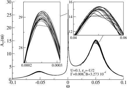
Figure 1: Spectral function $A_{\uparrow}(\omega)$ of the Anderson impurity model calculated for a range of $N$, the number of states kept in the truncation after each NRG iteration step. $N$ ranges from 1800 to 3600 in steps of 100. The Kondo temperature (defined as in Refs. Wilson, 1975; Krishna-murthy et al., 1980a) is $T_{K}=6.9\ 10^{-5}$, thus $B/T_{K}=4.7$.

In Fig. 1 we plot the spectral functions obtained in the calculations for a variable number of states kept, ranging from $N=1800$ (the value used in Ref. Schmitt and Anders, 2011a) up to $N=3600$. It has to be noted that even the lower limit $N=1800$ is sufficient to obtain essentially fully converged NRG results for static quantities (ground state energy, thermodynamic functions); the plot in Fig. 2 shows that at $N=1800$ the error in the calculated ground state energy is below $10^{-6}$, which is already a highly precise result. As evidenced in Fig. 1, the spectral functions, however, do not converge to some limiting curve as $N$ is increased. This is due to the way the spectral function is calculated in the CFS approach Peters et al. (2006); Weichselbaum and von Delft (2007): the delta-peak contributions appear at frequencies $\omega$ which are a difference of the energy of a kept state $E_{k}$ and the energy of a discarded state $E_{d}$, that is, $\omega=E_{d}-E_{k}$. While the kept states are in the part of the on-shell excitation spectrum which is expected to be rather accurate, thus $E_{k}$ is precise, the truncated states come from the top of the spectrum which is more significantly affected by the accumulated truncation errors from the previous NRG steps, thus the energies $E_{d}$ of these states are known to a lesser precision. In other words, in the CFS approach the normalization of the spectral function is guaranteed to be exactly 1, but the higher moments are not exact, i.e., only the 0-th spectral sum rule is fulfilled to numeric precision Peters et al. (2006); Žitko and Pruschke (2009). Increasing $N$ does not help in this respect, since this merely implies that a given excitation will contribute at a later NRG step, thus $E_{d}$ may accumulate even more truncation error. For this reason, changing $N$ will change the resulting spectrum. Since the states in the NRG are clustered, the changes can be relatively abrupt. (We note in passing that the spectral functions calculated using the patching approach converge as $N$ is increased, because one extracts the spectral information always from the same energy interval of the on-shell spectra, thus the effect of the truncation errors of the discarded states is tiny. Alas, the patching approach suffers from other deficiencies; in particular, there is a free parameter which needs to be tuned for each particular application, which limits the reliability of the approach.)

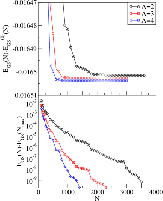
Figure 2: (Color online) Ground-state energy $E_{\mathrm{GS}}$ as a function of the number of states kept, $N$. $E_{\mathrm{GS}}$ is computed as described in Ref. Žitko, 2009. $E_{\mathrm{GS}}^{(0)}$ is the ground-state energy of the conduction band without the impurity, thus what is plotted is the impurity binding energy. The variation of the binding energy (in the large-$N$ limit) with $\Lambda$ is a direct consequence of the discretization errors. These results indicate the degree of convergence of the NRG calculation as a function of $N$ and $\Lambda$.

III Estimation of the spectral-function variance

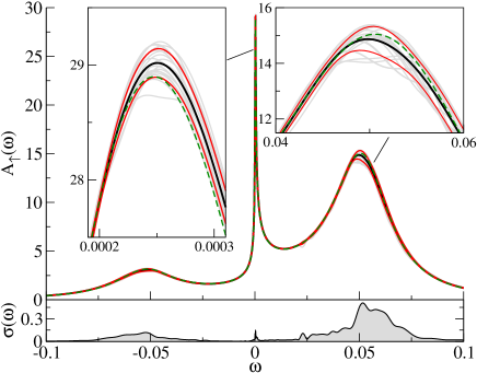
Figure 3: (Color online) Upper panel: Spectral function calculated by averaging the CFS spectra over all values of $N$ (thick black line) with a confidence interval determined by the standard deviation of the data at each $\omega$ (thinner lines/red online). For comparison, the spectral function calculated using the patching approach is also shown (dashed line/green online). The gray lines in the background are the individual CFS spectra from Fig. 1. Lower panel: standard deviation as a function of frequency.

Fig. 3 shows the spectral function $A(\omega)$ obtained by averaging over the curves shown in Fig. 1, together with the confidence region which represents the estimated range of values over which the spectral function fluctuates as a function of the truncation cutoff $N$. The confidence region is determined by calculating the standard deviation $\sigma(\omega)$ at each frequency $\omega$; the upper and lower boundaries of the region are then taken to be $A(\omega)\pm\sigma(\omega)$. For comparison, the spectral function calculated using the traditional patching approach is also shown; it is evident that this curve lies within or near the confidence region of the spectral function calculated using the CFS approach. In this sense, the two approaches appear equivalent in this case, however the patching approach by itself provides no means for estimating the reliability (i.e., the confidence region) of the result. The lower panel in Fig. 3 shows the standard deviation, $\sigma(\omega)$. It attains its highest values near the atomic peaks at $\omega\sim\epsilon_{d},\epsilon_{d}+U$ and it tends to decrease at lower frequencies, as expected, although it has a small local maximum at the Kondo resonance where the results are again more scattered.

From the results in Fig. 3 we extract the position of the Kondo resonance as the frequency of the maximum of the averaged spectral function, $\omega_{\mathrm{max}}=2.50\ 10^{-4}$. Let us consider now the estimation of the error committed due to the variance of the spectral functions. As a simple (albeit pessimistic) approximation we may consider that the true maximum is located anywhere within the triangle plotted in Fig. 4. The average width of the triangle is $(\omega_{B}-\omega_{A})/2$, thus the error estimate can be defined as

$$\delta\omega=\frac{\omega_{B}-\omega_{A}}{4}.$$ (2)

From the calculations for the discretization $\Lambda=2$ and the broadening $\alpha=0.075$ we thus conclude that the Kondo resonance is shifted by the external magnetic field to

$$\omega_{K}\approx 2.50\ 10^{-4}\ \pm\ 1.2\ 10^{-5}\approx 2.50\ 10^{-4}\ \left(1\pm 0.05\right),$$ (3)

or

$$\omega_{K}/b\approx 0.76\left(1\pm 0.05\right),$$ (4)

where $b=g\mu_{B}B$ is the magnetic field in energy units (Zeeman energy). In other words, using the NRG calculations at $\Lambda=2$, the position of the Kondo peak can be determined at best with 5% accuracy. This is the reason why it is so difficult to reliably study the dependence between the Kondo peak position and the external magnetic field, which should behave as $\omega_{K}=(2/3)b$ at low fields ($b\ll k_{B}T_{K}$) Logan and Dickens (2001); Hewson et al. (2006) and as $\omega_{K}=b$ at high fields Costi (2000); Moore and Wen (2000); Konik et al. (2001); Rosch et al. (2003); Hewson et al. (2006); Meir et al. (1993) ($b\gg k_{B}T_{K}$, but $B$ still small compared to the atomic parameters of the model, otherwise non-universal features are observed Žitko et al. (2009); Schmitt and Anders (2011a)).

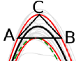
Figure 4: (Color online) Estimation of the true position of the peak maximum; see the text for details. The data is taken from the left inset in Fig. 3.

To gain more insight into the origin of the variation of the spectral function with $N$, in Fig. 5 we plot the raw binned spectral data for a fine-grained set of 256 different $z$ values. A comparison of the results for $N=2000$ and $N=3000$ shows that while the general aspects do not vary with $N$, the details do. The differences in these details lead to the variation of the spectral function with increasing $N$.

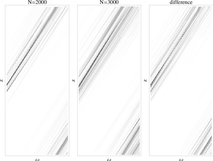
Figure 5: Raw binned spectral data in the energy range of the Kondo peak for a fine-grained range of $z$ values ($N_{z}=256$). These are raw spectral weights of the delta peaks forming the spectral functions which have been binned (logarithmic mesh, $600$ bins per decade; the intervals of the binning grid are much narrower than the broadening kernels used to post-processes these raw results). Left and middle panels show results for $N=2000$ and $N=3000$, while the right panel shows the difference between the two. The grayscale ranges are approximately equal in the three plots. In the plots $z$ ranges from 0 to 1 (bottom to top) and $\omega$ ranges from $0.0002$ to $0.0003$ (across the Kondo peak). The model parameters are as in Fig. 1.

IV Spectral function broadening

We now discuss the role of the spectral function broadening parameter $\alpha$ which is used to obtain smooth spectral curves from the spectral information in the form of weighted delta peaks. The broadening kernel used is

$$P(\omega,\omega^{\prime})=\frac{\theta(\omega\omega^{\prime})}{\sqrt{\pi}\alpha|\omega|}\exp\left[-\left(\frac{\log|\omega/\omega^{\prime}|}{\alpha}-\frac{\alpha}{4}\right)^{2}\right],$$ (5)

i.e., the broadening kernel proposed in Ref. Weichselbaum and von Delft, 2007 with $\gamma=\alpha/4$. The peak of this kernel function is located at

$$\omega=e^{-\alpha^{2}/4}\omega^{\prime}.$$ (6)

The weight is distributed asymmetrically with respect to $\omega^{\prime}$ with $1/2[1+\mathrm{erf}(\alpha/4)]$ of the weight in the interval $|\omega|>|\omega^{\prime}|$ and $1/2[1-\mathrm{erf}(\alpha/4)]$ in the interval $|\omega|<|\omega^{\prime}|$, where $\mathrm{erf}$ is the error function. Furthermore, the tail of the broadening function reaches to relatively high frequencies if $\alpha$ is large, thus the presence of high-energy spectral features might lead to spurious shifts of the peak positions in the low-energy part of the spectrum, and vice versa.

Naively, one could expect that increasing $\alpha$ will reduce the variance of the spectral curves. This is only partially true: the irregularities indeed smooth out, however the overall spectral weight distribution is still found to be fluctuating with $N$. Surprisingly, it is found that that $\delta\omega_{K}$, the estimated (pessimistic) error in the Kondo peak position, remains roughly constant with $\alpha$, see Fig. 6 for $\Lambda=2$. It is thus important to use a small broadening parameter to avoid systematic overbroadening errors Schmitt and Anders (2011a); Zhang et al. (2010). Clearly, a suitably small $\alpha$ is such that the overbroadening error is smaller than the intrinsic error due to the discretization (for instance, no larger than $\alpha=0.2$ or $\alpha=0.3$ in our example, see Fig. 6). The broadened spectral functions depend on the broadening kernel used; only in the limit of very small broadening widths do the different broadening kernels (Gaussian, log-Gaussian, modified log-Gaussian) all become equivalent. For moderate and large broadening, it was found that the modified log-Gaussian kernel works best, see Fig. 19 in Ref. Žitko and Pruschke, 2009.

It may be noted that the variance does not depend on the choice of the discretization scheme, because for the chosen model parameters and $\Lambda=2$, the discretization artifacts are small in any discretization scheme.

Figure 6: (Color online) The Kondo peak position (with “pessimistic” error bars) as a function of the broadening parameter. The (average) peak position is extracted by determining the maximum of the average of the spectral functions for different $N$; the maximum is located using the conjugate gradient method. The smallest $\alpha$, for which the Kondo peak maximum can still be extracted, is determined by the number $N_{z}$ of different values of the twist parameter (here $N_{z}=12$, and $\alpha_{\mathrm{min}}\approx 0.05$). For completeness, the results for larger broadening parameters $\Lambda=3$ and $\Lambda=4$ are also shown; smaller error-bars result from the fact that for coarser broadening the truncation errors decrease (while the discretization errors increase). Thus larger values of $\Lambda$ actually lead to less scatter in the calculated spectral functions as $N$ is varied.

Alternatively, one can determine the error in the extracted Kondo peak position by locating the maximum for each spectral function calculated at fixed $N$, and calculating the standard deviation. The results of such a calculation are shown in Fig. 7. The error bars are significantly smaller using this definition and they decrease with increasing $\alpha$. We can describe this procedure as “optimistic”, since it is found that the spectral functions with different $N$ in fact have their maxima at positions which fluctuate less that the curve does overall, thus the error bars are significantly smaller than in the “pessimistic” case presented in Fig. 6. The true systematic error probably lies somewhere between these two extreme error estimates, thus a suitable value of $\alpha$ for performing calculations aiming towards high-precision results is smaller than suggested by the error bars in Fig. 6, i.e., the broadening parameter should probably be closer to $\alpha=0.1$, rather than $\alpha=0.2$ or $0.3$, as suggested above.

Figure 7: (Color online) The Kondo peak position (with “optimistic” error bars) as a function of the broadening parameter. The peak position is extracted as an average of the maxima of the spectral functions for different $N$; each maximum is located using the conjugate gradient method. The error bars are determined by calculating the standard deviation of the extracted values for $\omega_{K}$. The error bars increase significantly for $\alpha<0.1$ because at given number of the twist parameters, $N_{z}=12$, the oscillations in the spectral functions become severe for $\alpha\lesssim 1/\sqrt{\Lambda}N_{z}$.

It is interesting to note that the effect of finite $\alpha$ is larger than expected from the shift described by Eq. (6). A good fit to the results for $\Lambda=2$ in Figs. 6 and 7 is

$$\omega_{K}(\alpha)=\omega_{K}(0)e^{-\alpha^{2}/b}$$ (7)

with $b\approx 2.25$. Thus the functional form of the shift is similar to that of Eq. (6), however the numerical factor in the argument of the exponential function is $2.25$ rather than $4$, i.e., the shift is even larger than expected. Test calculations for a single Lorentzian peak indeed show that spectral peaks with a finite width are broadened into a wider peak whose maximum is displaced by a factor of $e^{-\alpha^{2}/b}$ with $b$ smaller than 4. This is another reason for reducing $\alpha$ as far as possible.

V Kondo resonance splitting

As an application, we now consider the problem of the Kondo resonance splitting in an external magnetic field. We plot the splitting ratio $\omega_{K}/(g\mu_{B}B)$ as a function of the ratio $g\mu_{B}B/k_{B}T_{K}$ in Fig. 8. (Note that $\omega_{K}$ is defined as the shift of the Kondo peak position in the spin-projected spectral function $A_{\sigma}(\omega)$ and that the peak-to-peak distance in the spin-averaged spectral function is not exactly $2\omega_{K}$.) Both procedures for extracting the average value and the error bars have been performed. The average values (circles and squares in the figure) agree within the error bars of the ”optimistic procedure” for all the results shown; deviation becomes larger for smaller magnetic fields. For large fields, the ratio increases in a rather slow (logarithmic) way, thus one expects non-universal features to appear before the universal high-field asymptotic behavior is reached. For small fields, the ratio goes toward a value of 0.7, which is close to the expected low-field limit value Logan and Dickens (2001); Hewson et al. (2006) of 2/3. [The low-field asymptotic limit has been reported to be confirmed in a calculation where broadening is performed using Lorentzian peaks with constant width at very low energy scales Hewson et al. (2006).] The ”pessimistic” error bars grow larger for small fields, and the ”optimistic” average values start to deviate from the ”pessimistic” ones. This is expected, since the Kondo peak displacement becomes smaller than the Kondo peak width, thus the relative errors (i.e., the error of the ratio $\omega_{K}/g\mu_{B}B$) grow with decreasing $B$ because the absolute error $\delta\omega_{K}$ approximately saturates for $g\mu_{B}B\ll k_{B}T_{K}$.

Figure 8: (Color online) The Kondo resonance splitting as a function of the external magnetic field. The error bars correspond to the ”pessimistic” and ”optimistic” error estimates. Model parameters are $U=0.1$, $\epsilon_{d}=-U/2$, $\Gamma=0.008$ in units of half-bandwidth of the (flat) conduction band. The broadening parameter is $\alpha=0.075$. The data labeled as “Moore Wen” are taken from Fig. 2 in Ref. Moore and Wen, 2000.

The results in Fig. 8 are in good agreement with the splitting in the Kondo model as determined from the spinon density of states in the Bethe Ansatz (BA) solution Moore and Wen (2000), see the full line with crosses in Fig. 8. At large fields, the deviation beyond the error bars is most likely due to the differences between Anderson and Kondo models at high fields which leads to non-universal features. At low fields, we can say, at most, that the NRG and BA results are consistent within the errorbars. This trend is also found in experimental results Quay et al. (2007). In experiments where the splitting was found to exceed the predicted splitting in the high-field range Kogan et al. (2004); Liu et al. (2009), this is likely due to the non-universal effects which are expected in systems which are not in the extreme Kondo limit, i.e., the regime where the Kondo temperature is lower by many orders of the magnitude compared to all other energy scales in the problem. Such non-universal effects are expected in the Anderson model Schmitt and Anders (2011a), but also in the Kondo model Žitko et al. (2009). Furthermore, one should take into account the strong asymmetry of the Kondo peaks in strong magnetic field: perturbative renormalization group calculations Rosch et al. (2003) show that the maximum of the spectral peak is located at $\omega>g\mu_{B}B$, while the center of the left flank of the peak appears to be position almost precisely at $\omega=g\mu_{B}B$. For very large fields, the peak itself is no longer observable and one is left with a step in the spectral function, which should be considered as the sole remnant of the Kondo resonance. Finally, it should also be noted that for meaningful comparison with the experimental results, it is necessary to take into account the non-equilibrium effects if the splitting is extracted from the conductance at finite source-drain voltage in quantum-dot setups with symmetric coupling to both leads Hewson et al. (2005); Schmitt and Anders (2011b).

We are now in the position to critically discuss the recent work on the scaling of the magnetic-field-induced Kondo resonance splitting Zhang et al. (2010), the comment concerning that work Schmitt and Anders (2011a), and the reply offered by the authors of the original work Zhang et al. (2011). In particular, it has been claimed Zhang et al. (2010) that the position of the Kondo resonance in the total spectral function does not approach its position in the spin-resolved spectra for high magnetic fields, in contradiction to what has been found in some previous works Žitko et al. (2009), and that the splitting shows non-universal behavior even for modest $B/T_{K}$ ratio of order 10. Both conclusions have been shown in Ref. Schmitt and Anders, 2011a to be a consequence of the spectral function overbroadening due to an excessively large broadening parameter $\alpha=0.8$ and it was pointed out that different results are obtained with smaller broadening $\alpha=0.075$. In reply, it has been claimed that the value of $\alpha=0.075$ is too small and that $\alpha=0.4$ is a more appropriate choice Zhang et al. (2011).

The results of the present work, in particular Figs. 6 and 7, make it possible to go beyond the purported “certain arbitrariness” in the choice parameters Zhang et al. (2011) and elucidate to what extend the NRG can provide a definitive answer to the problem of the magnetic-field-induced Kondo peak splitting. Two points need to be emphasized: i) while $\alpha=0.8$ is clearly too large (it leads to an error in excess of 30% in determining the Kondo peak positions) and $\alpha=0.4$ is better (15% error), it is crucial to go in the $\alpha\to 0$ limit in order to obtain a result with accuracy in the percent range, thus $\alpha=0.075$ is a good choice for $N_{z}=12$; ii) using the “pessimistic” error estimate, there is a sizable overlap of the confidence regions for $\alpha=0.075$ and $\alpha=0.4$, thus there is non-negligible possibility that a calculation performed for a certain fixed value of $N$ would yield similar results for the peak position using both values of $\alpha$, see Fig. 6, although this conclusion is likely to be too pessimistic and a different error estimate suggest a clear difference between $\alpha=0.4$ and $\alpha=0.075$ results, see Fig. 7. It may be thus concluded that $\alpha=0.075$ is a more appropriate choice of the broadening parameter and that the results and conclusions of Ref. Zhang et al., 2010 are questionable due to spectral overbroadening. In particular, in the $\alpha\to 0$ limit, the Kondo peak positions in the total and spin-resolved spectral functions approach in the high-field limit Žitko et al. (2009); Schmitt and Anders (2011a). The conclusion of Ref. Zhang et al., 2010 that the slope coefficient of the ratio of the Kondo peak splitting over magnetic field is 2/3 in the small field limit, as expected Logan and Dickens (2001); Hewson et al. (2006), is surprising given the significant shift of the Kondo peak due to overbroadening; this result may be simply fortuitous. Using log-Gaussian broadening and taking into account the error bars in the small-$\alpha$ limit, such slope determination cannot be made in a reliable way using the NRG, see Fig. 8. Furthermore, it may also be remarked that the number of states kept in Ref. Zhang et al., 2010, i.e. $N=150$, is too small to obtain well converged results (see Fig. 2), irrespective of the broadening procedure used.

VI Inelastic (spin-flip) tunneling step and the large-field limit

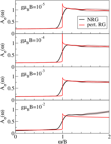
Figure 9: (Color online) Spectral function of the Anderson impurity model in high magnetic field, $B\gg T_{K}$. Black line corresponds to the NRG results, the two ligher (brown onlines) lines demarkate the confidence region, while the light (red online) curve corresponds to the analytical perturbative RG function from Ref. Rosch et al., 2003.

If $U$ is much larger than $\Gamma$, for instance $U/\Gamma=100$, the Kondo temperature is for all practical purposes equal to zero, since experiments are performed at a finite temperature which is, in this case, larger than $T_{K}$ by orders of magnitude. The impurity then behaves much like a free spin, as long as the external magnetic field is not comparable to the atomic energy scales ($\epsilon$, $U$). In experiments, for example in the inelastic spin-flip tunneling spectroscopy using a scanning tunneling miscroscope (STM) Heinrich et al. (2004), one can induce inelastic scattering by injecting electrons from the STM tip into the adsorbed impurity with energy exceeding the characteristic energy of a spin-flip event, i.e., above the Zeeman energy. Due to high relevance for STM experiments, it is of substantial interest to study the spectral function of the Anderson impurity model in the vicinity of the on-set of inelastic scattering. We study three aspects of this problem: i) the line-shape of the step in the spectral function at the on-set of spin-flip scattering; ii) the position of this step as $B$ approaches the atomic scales; iii) merging of the step with the atomic peak.

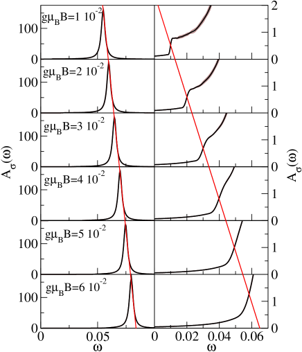
Figure 10: (Color online) Spectral function of the Anderson impurity model in very high magnetic field, $B\gg T_{K}$ and $B\sim U/2$. The dark lines are the averaged NRG results, while the lighter (brown online) lines indicate the confidence region. The discretization errors are more pronounced on the high-frequency side of the spectral step at $\omega=b\equiv g\mu_{B}B$.

We express the magnetic field in energy units (Zeeman splitting) as $b=g\mu_{B}B$. For $b$ small compared with the atomic scales, but $b\gg T_{K}$, we find that the spectral function around $\omega=b$ takes the form of a step, see Fig. 9. This regime has been studied before using both NRG and perturbative renormalization group (RG) techniques, see Fig. 5 in Ref. Rosch et al., 2003. Our results are consistent with these studies. Taking into account the finite broadening width in the NRG calculations, an excellent agreement is found with perturbative RG as long as $b$ is much smaller compared to $U$ (see the deviations for $b/U=1/5$, bottom-most panel in Fig. 9; note that the perturbative RG calculation is performed for the effective Kondo model, not for the Anderson model). In experiments, finite temperature will play a similar smoothing effect as spectral broadening in NRG, thus one can indeed expect to observe a step-like spectral line-shape. The step, whose center is always located at $\omega=b$, can be interpreted as the on-set of the inelastic (spin-flip) scattering, which is observed by the spin-flip spectroscopy in system that do not exhibit the Kondo effect Heinrich et al. (2004). It should be noted that there is no discernable peak at $\omega=b$: in this $b\gg T_{K}$ regime, the field-split Kondo resonance has become so asymmetric that it takes the form of a relatively sharp step Rosch et al. (2003). The width of the step as determined by the NRG matches that expected for a unit-step function broadened by the kernel, i.e., the intrinsic width of the step is very small, presumably equal to $\Gamma\approx\pi B/(16\ln^{2}[B/T_{K}])$, the transverse spin relaxation rate Rosch et al. (2003). We also point out that nothing noticeable happens on the scale $b\sim\Gamma=10^{-3}$, nor on the scale $b\sim\sqrt{U\Gamma}=10^{-2}$.

We now study the regime where $b$ is comparable to the atomic scales, Fig. 10. We again observe that there is always a spectral step exactly at $\omega=B$, see right panels in Fig. 9. The steps becomes more diffuse as it merges with the atomic peak for $b\gtrsim U/2$.

In the atomic limit ($\Gamma\to 0$), the impurity energy levels are

$$\begin{split}E_{0}&=0,\\ E_{\uparrow}&=\epsilon+b/2,\\ E_{\downarrow}&=\epsilon-b/2,\\ E_{2}&=2\epsilon+U.\end{split}$$ (8)

In the particle-hole symmetric point, $\delta=\epsilon+U/2=0$, one has $E_{2}=E_{0}$, thus for any non-zero value of the magnetic field, the state $|\downarrow\rangle$ is the ground state and the spin-up spectral function has a peak at

$$\omega_{0}=E_{2}-E_{\downarrow}=\epsilon+U+b/2=\delta+U/2+b/2.$$ (9)

We find that for $b\gtrsim U$, the peak position indeed deviates only little from $\omega_{0}$, see left panels in Fig. 10.

VII Conclusion

An analysis of the spectral functions calculated using the NRG technique shows that there is always some variance due to the discretization and truncation errors. For the range of values of $N$ which is suitable for practical NRG calculations, the obtained spectral functions do not converge; instead, the variance of the truncation errors appears to be approximately constant as a function of $N$ (for large $N$). Using a large broadening parameter does not solve the problem, but merely masks it. Furthermore, overbroadening errors appear to be a much larger reason for concern than the discretization and truncation errors. Accurate calculations should therefore aim for obtaining the results in the limit of zero broadening width, taking into account the constraints imposed by the systematic NRG errors. Errors should be quantified, not ignored.

We applied the procedure to estimate the errors in the NRG results for the Kondo resonance splitting in the external magnetic field. The systematic errors preclude the study of the small-field limit. For intermediate fields, however, it is possible to calculate the splitting ratio $\omega_{K}/g\mu_{B}B$ with an estimated error of a few percent, which is reasonably accurate. Good agreement is found with the Bethe Ansatz results for the peak splitting by Moore and Wen Moore and Wen (2000) in the regime of small and intermediate magnetic fields, where Anderson and Kondo models are equivalent.

To find a definitive quantitative solution of the problem of the Kondo resonance splitting in the external magnetic field, it will be necessary to devise numerical techniques that can reduce the discretization and truncation artifacts even further. Recent developments where the NRG matrix product state representation is refined using the density-matrix renormalization group (DMRG) procedure or variationally Weichselbaum et al. (2009); Pižorn and Verstraete (2011) may be very valuable in this respect since they might allow performing calculation at much reduced discretization parameters $\Lambda$ and optimizing the excited state energies by sweeping.