Asymptotics and Computation of the Solution to the Conductivity Equation in the Presence of Adjacent Inclusions with Extreme Conductivities

Abstract

When inclusions with extreme conductivity (insulator or perfect conductor) are closely located, the gradient of the solution to the conductivity equation can be arbitrarily large. And computation of the gradient is extremely challenging due to its nature of blow-up in a narrow region in between inclusions. In this paper we characterize explicitly the singular term of the solution when two circular inclusions with extreme conductivities are adjacent. Moreover, we show through numerical computations that the characterization of the singular term can be used efficiently for computation of the gradient in the presence adjacent inclusions.

Mathematics subject classification (MSC2000): 35J25, 73C40

Keywords: conductivity equation, anti-plane elasticity, stress, blow-up, extreme conductivity

1 Introduction

Frequently in composites which consist of inclusions and background (the matrix), the inclusions are closely spaced, and it is quite important from a practical point of view to know whether the gradient of the potential can be arbitrarily large as the inclusions get closer to each other. The gradient of the potential represents the stress in anti-plane elasticity and the electric field in the conductivity problem; see [6]. It is known that the gradient of the potential may blow up as the distance between the inclusions goes to zero and their material parameters (conductivities or stiffness) degenerate.

Suppose that $B_{1}$ and $B_{2}$ are inclusions whose conductivity is $k$. We suppose that the conductivity of the background is $1$ ($k\neq 1$). Let $\epsilon$ be the distance between $B_{1}$ and $B_{2}$ and assume that $\epsilon$ is small. The problem is to estimate $|\nabla u|$, where $u$ is the electrical potential, in terms of $\epsilon$ when $\epsilon$ tends to $0$.

There have been important works on this problem. If $k$ stays away from $0$ and $\infty$, i.e., $c_{1}<k<c_{2}$ for some positive constants $c_{1}$ and $c_{2}$, then it was proved by Bonnetier-Vogelius [10] and Li-Vogelius [19] that $|\nabla u|$ remains bounded regardless of $\epsilon$. This result was extended to elliptic system by Li-Nirenberg [18]. It is worth emphasizing that the results in [19, 18] are not only for two inclusions case but also for the case of arbitrary number of inclusions.

On the other hand, if $k$ is either $0$ (insulating) or $\infty$ (perfectly conducting), then $\nabla u$ may blow up as $\epsilon$ tends to $0$. For two identical perfectly conducting circular inclusions it was shown in [7] (see also [17] and [16]) that the gradient in general becomes unbounded as $\epsilon$ approaches zero and the blow-up rate is $\epsilon^{-1/2}$. In [3, 4], a lower bound and an upper bound for the gradient has been obtained. These bounds are valid for all $k$ including extreme values ($k=0$ and $k=\infty$) and provide the precise dependence of $\nabla u$ on $\epsilon$, $k$ and radii of disks. The blow-up of the gradient may or may not occur depending on the background potential. In [5], Ammari et al characterize those background potential which actually make the gradient blow up. In [22, 23], Yun showed that the blow-up rate is $\epsilon^{-1/2}$ for perfectly conducting and insulated inclusions of arbitrary shape in two dimensions. In three dimensions, Bao et al [8] proved that the blow-up rate for the perfectly conducting inclusions is $|\epsilon\log\epsilon|^{-1}$ and extended the result to the case of multiple inclusions [9]. Lim-Yun [20] also found the same blow-up rate when inclusions are spheres. Their estimates explicitly reveal the dependence on the radii of the sphere. They also showed in [21] that if there is a small bump in between two inclusions in two dimensions, then the magnitude of the blow-up gets larger.

The purpose of this paper is to characterize the singular term of the solution, i.e., to establish an asymptotic formula for the blow-up of the gradient when two circular inclusions get closer. We find the decomposition of the solution $u$ to the conductivity equation as

$$u=g+b$$ (1.1)

where $\nabla g$ may blow up at the rate of $\epsilon^{-1/2}$ while $\nabla b$ stays bounded regardless of $\epsilon$, when $B_{1}$ and $B_{2}$ are disks and $k$ is either $\infty$ or $0$. We actually obtain an explicit formula for the term $g$ which gives a precise description of singular behavior of $\nabla u$.

The characterization of the singular term of the solution finds a very good application in the computation of electrical fields. Computation of the electrical field in the presence of closely located inclusions with extreme ($0$ or $\infty$) conductivities is known to be a extremely difficult problem because of the the blow-up phenomenon in a very narrow region between inclusions. Since the the gradient of the solution is arbitrarily large, we need very fine mesh to catch the large gradient in a narrow region. The results of this paper constitute a significant step toward overcoming this difficulty since the singular term $g$ is explicit and computation of $b$ requires only regular meshes. We present efficient methods to use the decomposition for the computation of the solution and some results of numerical computation using them. Numerical examples of this paper show that these methods work pretty well.

This paper is organized as follows. In the next section we derive the decomposition (1.1) for the perfect conductors in the free space. In section 3, we deal with the same problem in bounded domains. Section 4 is for the insulators. New numerical methods and results of computation are presented in the last section.

The result of this paper can be extended to perfect conductors of spherical shape in three dimensions. This result will be presented in a forthcoming paper.

2 Free space problem-perfectly conducting case

Let $B_{j}=B({\bf c}_{j},r_{j})$, $j=1,2$, be the disk centered at ${\bf c}_{j}$ and of radius $r_{j}$, and

$$\sigma=\left\{\begin{aligned} &1\quad\mbox{on }\mathbb{R}^{2}\setminus(B_{1}\cup B_{2}),\\ &k\quad\mbox{on }B_{1}\cup B_{2},\end{aligned}\right.$$ (2.1)

which represents the conductivity distribution: the conductivity of the inclusions is $k$ ($k\neq 1$) and that of the background is 1. The equation we consider is

$$\nabla\cdot\sigma\nabla u=0\quad\mbox{in }\mathbb{R}^{2},$$ (2.2)

which may be viewed as the conductivity equation or anti-plane elasticity equation. A condition at the infinity is prescribed by

$$u({\bf x})-H({\bf x})=O(|{\bf x}|^{-1})\quad\mbox{as }|{\bf x}|\to\infty,$$ (2.3)

where $H$ is an entire harmonic function and represents the background potential.

If $k=\infty$, the equation (2.2) with the condition (2.3) is understood as the following problem:

$$\left\{\begin{array}[]{ll}\displaystyle\Delta u=0&\mbox{in }{\mathbb{R}^{2}\setminus\overline{B_{1}\cup B_{2}}},\\ \displaystyle u|_{\partial B_{j}}=\lambda_{j}\ (\mbox{constant})&j=1,2,\\ \displaystyle u({\bf x})-H({\bf x})=O(|{\bf x}|^{-1})&\mbox{as }|{\bf x}|\rightarrow\infty.\end{array}\right.$$ (2.4)

The constants $\lambda_{j}$ can be determined by the additional requirements

$$\int_{\partial B_{j}}\frac{\partial u}{\partial\nu}\Big{|}_{+}~{}ds=0,\quad j=1,2,$$ (2.5)

where $\nu$ is the outward unit normal vector of ${\mathbb{R}^{2}\setminus\overline{B_{1}\cup B_{2}}}$, i.e., directed inward of $B_{i}$. Here and throughout this paper, the notations $|_{+}$ and $|_{-}$ are for limits from outside and inside inclusions, respectively.

Let $R_{j}$, $j=1,2$, be the reflection with respect to $\partial B_{j}$, i.e.,

$$R_{j}({\bf x}):=\frac{r_{j}^{2}({\bf x}-{\bf c}_{j})}{|{\bf x}-{\bf c}_{j}|^{2}}+{\bf c}_{j},\quad j=1,2.$$ (2.6)

It is easy to see that the combined reflections $R_{1}R_{2}$ and $R_{2}R_{1}$ have unique fixed points, say ${\bf p}_{1}$ and ${\bf p}_{2}$, respectively. Let

$$h({\bf x}):=\frac{1}{2\pi}\left(\log|{\bf x}-{\bf p}_{1}|-\log|{\bf x}-{\bf p}_{2}|\right).$$ (2.7)

The function $h$, which was first found in [20], has a special property: it is the solution to

$$\begin{cases}\displaystyle\Delta h=0\quad&\mbox{in }\mathbb{R}^{2}\setminus\overline{B_{1}\cup B_{2}},\\ \displaystyle h|_{\partial B_{j}}=C_{j}\ (\mbox{constant})\quad&j=1,2,\\ \vskip 6.0pt plus 2.0pt minus 2.0pt\cr\displaystyle\int_{\partial B_{j}}\frac{\partial h}{\partial\nu}~{}ds=(-1)^{j},\quad&j=1,2,\\ \displaystyle h({\bf x})=O(|{\bf x}|^{-1})\quad&\mbox{as }|{\bf x}|\to\infty.\end{cases}$$ (2.8)

The following formula was proved in [22, 23]: let $\lambda_{1}$ and $\lambda_{2}$ be constants appearing in (2.4), then

$$\lambda_{2}-\lambda_{1}=\int_{\partial B_{1}\cup\partial B_{2}}H\partial_{\nu}h~{}ds=H(\textbf{p}_{2})-H(\textbf{p}_{1}).$$ (2.9)

The following is the first main theorem of this paper.

Theorem 2.1

Let ${\bf n}$ be the unit vector in the direction of ${\bf p}_{2}-{\bf p}_{1}$ and let ${\bf p}$ be the middle point of the shortest line segment connecting $\partial B_{1}$ and $\partial B_{2}$. For a harmonic function $H$ in $\mathbb{R}^{2}$, let $u$ be the solution to (2.4). Then, the solution $u$ can be expressed as follows:

$$u({\bf x})=ah({\bf x})+b({\bf x})$$ (2.10)

where

$$a=\frac{4\pi r_{1}r_{2}}{r_{1}+r_{2}}({\bf n}\cdot\nabla H)({\bf p})$$ (2.11)

and for any bounded set $\Omega$ containing $\overline{B}_{1}$ and $\overline{B}_{2}$ there is a constant $C$ independent of $\epsilon$ such that

$$\|\nabla b\|_{L^{\infty}(\Omega\setminus(B_{1}\cup B_{2}))}\leq C.$$ (2.12)

The asymptotic formula $\nabla u$ as $\epsilon\to 0$ is then given by

$$\nabla u({\bf x})=\frac{2r_{1}r_{2}}{r_{1}+r_{2}}({\bf n}\cdot\nabla H)({\bf p})\left(\frac{\mathbf{x}-\mathbf{p}_{1}}{\bigr{|}\mathbf{x}-\mathbf{p}_{1}\bigr{|}^{2}}-\frac{\mathbf{x}-\mathbf{p}_{2}}{\bigr{|}\mathbf{x}-\mathbf{p}_{2}\bigr{|}^{2}}\right)+O(1).$$ (2.13)

Let us make a few remarks on Theorem 2.1 before proving it. It is shown in [22, 23] that the fixed points ${\bf p}_{1}$ and ${\bf p}_{2}$ are given by

$${\bf p}_{1}=\Bigr{(}-\sqrt{2}\sqrt{\frac{r_{1}r_{2}}{r_{1}+r_{2}}}\sqrt{\epsilon}+O(\epsilon),0\Bigr{)}\quad\mbox{and}\quad{\bf p}_{2}=\Bigr{(}\sqrt{2}\sqrt{\frac{r_{1}r_{2}}{r_{1}+r_{2}}}\sqrt{\epsilon}+O(\epsilon),0\Bigr{)}$$

if $\mathbf{c}_{1}=(-r_{1}-\frac{\epsilon}{2},0)$ and $\mathbf{c}_{2}=(r_{2}+\frac{\epsilon}{2},0)$. If $r_{1}$ and $r_{2}$ are bounded below by a positive constant $r_{0}$, then there are positive constants $C_{1}$ and $C_{2}$ depending only on $r_{0}$ such that

$$C_{1}\sqrt{\frac{r_{1}+r_{2}}{r_{1}r_{2}}}\frac{1}{\sqrt{\epsilon}}\leq|\nabla h({\bf x})|\leq C_{2}\sqrt{\frac{r_{1}+r_{2}}{r_{1}r_{2}}}\frac{1}{\sqrt{\epsilon}}$$ (2.14)

for all ${\bf x}$ on the the shortest line segment connecting $\partial B_{1}$ and $\partial B_{2}$, see [21]. Thus the blow-up rate of $|\nabla u|$ is $\epsilon^{-1/2}$. It is also proved in the same paper that

$$|\nabla h({\bf x})|\leq C\sqrt{\frac{r_{1}+r_{2}}{r_{1}r_{2}}}\frac{1}{\sqrt{\epsilon}}$$ (2.15)

for all ${\bf x}$. Thus, an optimal bound for $\nabla u$ in a bounded domain can be obtained from (2.14) and (2.15) in terms of $r_{1}$, $r_{2}$, $\epsilon$ and $({\bf n}\cdot\nabla H)({\bf p})$. In view of the formula (2.11) of $a$ (we call it the stress intensity factor), the blow-up does not occur if $({\bf n}\cdot\nabla H)({\bf p})=0$. This fact was already found in [5]. One can also show that if $r_{1}$ and $r_{2}$ are $O(\epsilon)$, then there is a constant $C$ independent of $\epsilon$ such that

$$|\nabla h({\bf x})|\leq\frac{C}{\epsilon}$$ (2.16)

for all ${\bf x}$. Thus (2.13) means that in this case, no blow-up occurs: $\nabla u$ stays bounded. This finding is in agreement with that in [4].

We first prove the following proposition by modifying an argument of Bao et al [8].

Proposition 2.2

Let

$$b({\bf x})=u({\bf x})-\left(\frac{u|_{\partial B_{2}}-u|_{\partial B_{1}}}{h|_{\partial B_{2}}-h|_{\partial B_{1}}}\right)h({\bf x}),\quad{\bf x}\in\mathbb{R}^{2}\setminus(B_{1}\cup B_{2}).$$ (2.17)

For any bounded set $\Omega_{1}$ containing $\overline{B}_{1}$ and $\overline{B}_{2}$ and $\Omega_{2}$ containing $\overline{\Omega}_{1}$, there is a constant $C$ independent of $\epsilon$ such that

$$\|b\|_{\mathcal{C}^{1}(\Omega_{1}\setminus{(B_{1}\cup B_{2})})}\leq C\|H\|_{L^{\infty}(\Omega_{2})}.$$ (2.18)

Proof.   It can be easily seen that $b$ is bounded. In fact, since $b$ is harmonic in $\mathbb{R}^{2}\setminus\overline{B_{1}\cup B_{2}}$ and

$$b|_{\partial B_{2}}-b|_{\partial B_{1}}=0,$$

we infer from the result in [1] (see also [8]) that $b$ is bounded in $\Omega_{1}$.

Since $h({\bf x})\to 0$ as $|{\bf x}|\to\infty$, by the maximum principle, $h$ attains its maximum and minimum on $\partial B_{2}$ and $\partial B_{1}$, respectively. Thus, we have

$$\|h\|_{L^{\infty}(\mathbb{R}^{2}\setminus(B_{1}\cup B_{2}))}\leq h|_{\partial B_{2}}-h|_{\partial B_{1}},$$

and hence

$$\|b\|_{L^{\infty}(\Omega_{2}\setminus{(B_{1}\cup B_{2})})}\leq\|u\|_{L^{\infty}(\Omega_{2}\setminus(B_{1}\cup B_{2}))}+\left|u|_{\partial B_{2}}-u|_{\partial B_{1}}\right|.$$ (2.19)

Let $\lambda_{j}=u|_{\partial B_{j}}$, $j=1,2$, and assume that $\lambda_{2}\geq\lambda_{1}$ without loss of generality. Since $(u-H)({\bf x})\to 0$ as $|{\bf x}|\to\infty$, the maximum and minimum of $u-H$ occur on $\partial B_{1}\cup\partial B_{2}$. So, we have

$$(u-H)({\bf x})\leq\max_{\partial B_{1}\cup\partial B_{2}}(u-H)\leq\lambda_{2}+\|H\|_{L^{\infty}(\Omega_{2})},$$

and

$$\lambda_{1}-\|H\|_{L^{\infty}(\Omega_{2})}\leq\min_{\partial B_{1}\cup\partial B_{2}}(u-H)\leq(u-H)({\bf x})$$

for all ${\bf x}\in\mathbb{R}^{2}\setminus({B_{1}\cup B_{2}})$. Since $\min_{\mathbb{R}^{2}\setminus(B_{1}\cup B_{2})}(u-H)\leq 0$, we have

$$\lambda_{1}\leq\|H\|_{L^{\infty}(\Omega_{2})}.$$

Therefore, we have

$$\|u-H\|_{L^{\infty}(\Omega_{2}\setminus(B_{1}\cup B_{2}))} \leq\lambda_{2}+\|H\|_{L^{\infty}(\Omega_{2})}$$

$$\leq\lambda_{2}-\lambda_{1}+2\|H\|_{L^{\infty}(\Omega_{2})}\leq 4\|H\|_{L^{\infty}(\Omega_{2})},$$

where the last inequality comes from (2.9). Thus

$$\|u\|_{L^{\infty}(\Omega_{2}\setminus{(B_{1}\cup B_{2})})}\leq\|H\|_{L^{\infty}(\Omega_{2})}+\|u-H\|_{L^{\infty}(\Omega_{2}\setminus{(B_{1}\cup B_{2})})}\leq 5\|H\|_{L^{\infty}(\Omega_{2})}.$$

It then follows from (2.19) and (2.9) that

$$\|b\|_{L^{\infty}(\Omega_{2}\setminus(B_{1}\cup B_{2}))}\leq 7\|H\|_{L^{\infty}(\Omega_{2})}.$$ (2.20)

We now show that

$$\|\nabla b\|_{L^{\infty}(\Omega_{1}\setminus(B_{1}\cup B_{2}))}\leq C\|H\|_{L^{\infty}(\Omega_{2})}.$$ (2.21)

For that purpose, we define the harmonic functions $G_{+}$ and $G_{-}$ as follows:

$$\quad\left\{\begin{array}[]{ll}\displaystyle\Delta G_{\pm}=0,&\mbox{in }{\Omega_{2}\setminus\overline{B_{1}\cup B_{2}}},\\ \displaystyle G_{\pm}=\pm\|b\|_{L^{\infty}(\Omega_{2}\setminus(B_{1}\cup B_{2}))}&\mbox{on }\partial\Omega_{2},\\ \displaystyle G_{\pm}=b,&\mbox{on }\partial B_{1}\cup\partial B_{2}.\end{array}\right.$$

Then, $\pm(G_{\pm}-b)\geq 0$ in $\Omega_{2}\setminus\overline{B_{1}\cup B_{2}}$ and $G_{\pm}-b=0$ on $\partial B_{1}\cup\partial B_{2}$. By Hopf’s Lemma, we have

$$\partial_{\nu}G_{+}\leq\partial_{\nu}b\leq\partial_{\nu}G_{-}\quad\mbox{on}~{}\partial B_{1}\cup\partial B_{2}.$$ (2.22)

We introduce more harmonic functions $G_{+1}$, $G_{+2}$, $G_{-1}$ and $G_{-2}$ defined as follows: for $i=1,~{}2$,

$$\quad\left\{\begin{array}[]{ll}\displaystyle\Delta G_{\pm i}=0,&\mbox{in }{\Omega_{2}\setminus\overline{B_{i}}},\\ \displaystyle G_{\pm i}=G_{\pm}=\pm\|b\|_{L^{\infty}(\Omega_{2}\setminus(B_{1}\cup B_{2}))}&\mbox{on }\partial\Omega_{2},\\ \displaystyle G_{\pm i}=G_{\pm}=b,&\mbox{on }\partial B_{i}.\end{array}\right.$$

Since $b|_{\partial B_{1}}=b|_{\partial B_{2}}=\mbox{constant}$, we have

$$G_{+i}({\bf x})\geq b|_{\partial B_{1}\cup\partial B_{2}}.$$

In particular,

$$G_{+i}({\bf x})\geq b({\bf x})=G_{+}({\bf x})\quad\mbox{on }\partial B_{1}\cup\partial B_{2}.$$

Since $G_{+i}|_{\partial\Omega_{2}}=G_{+}|_{\partial\Omega_{2}}$, we have

$$G_{+i}-G_{+}\geq 0\quad\mbox{in }\Omega_{2}\setminus{B_{1}\cup B_{2}}.$$

Since $G_{+i}-G_{+}=0$ on $\partial B_{i}$, it follows from the Hopf’s Lemma that

$$\partial_{\nu}G_{+i}\leq\partial_{\nu}G_{+}\quad\mbox{on }\partial B_{i},\ \ i=1,2.$$ (2.23)

Similarly, one can show that

$$\partial_{\nu}G_{-i}\geq\partial_{\nu}G_{-}\quad\mbox{on }\partial B_{i},\ \ i=1,2.$$ (2.24)

Note that ${G_{\pm 1}}/{\|b\|_{L^{\infty}(\Omega_{2}\setminus(B_{1}\cup B_{2}))}}$ is a harmonic function in $\Omega_{2}\setminus\overline{B_{1}}$ which is $\pm 1$ on $\partial\Omega_{2}$ and also has a constant value between $-1$ and $1$ on $\partial B_{1}$, and that $\mbox{dist}({B_{1},\partial\Omega_{2}})>c_{0}$. Thus, ${G_{\pm 1}}/{\|b\|_{L^{\infty}(\Omega_{2}\setminus(B_{1}\cup B_{2}))}}$ can be extended as a harmonic function into $\Omega_{2}\setminus\overline{B({\bf c}_{1},\tilde{r})}$ where ${\bf c}_{1}$ is the center of $B_{1}$ and $\tilde{r}$ is strictly less than the radius of $B_{1}$ independently of $\epsilon$. Then, we have from interior regularity estimates for elliptic equations and (2.20) that

$$\|\partial_{\nu}G_{\pm 1}\|_{L^{\infty}(\partial B_{1})}\leq C\|b\|_{L^{\infty}(\Omega_{2}\setminus(B_{1}\cup B_{2}))}\leq 7C\|H\|_{L^{\infty}(\Omega_{2})}.$$

It then follows from (2.22), (2.23) and (2.24) that

$$\|\partial_{\nu}b\|_{L^{\infty}(\partial B_{1})}\leq C\|H\|_{L^{\infty}(\Omega_{2})}$$

for some constant $C$ independent of $\epsilon$. Similarly one can show that

$$\|\partial_{\nu}b\|_{L^{\infty}(\partial B_{2})}\leq C\|H\|_{L^{\infty}(\Omega_{2})}.$$

Since $b$ is constant on $\partial B_{1}$ and $\partial B_{2}$, we get

$$\|\nabla b\|_{L^{\infty}(\partial B_{1}\cup\partial B_{2})}\leq C\|H\|_{L^{\infty}(\Omega_{2})}.$$ (2.25)

The standard interior regularity estimate for harmonic functions shows that

$$\|\nabla b\|_{L^{\infty}(\partial\Omega_{1})}\leq C\|H\|_{L^{\infty}(\Omega_{2})}.$$

The maximum principle now yields (2.21), and the proof is complete. $\square$

We are now ready to prove Theorem 2.1.

Proof of Theorem 2.1. After translation and rotation if necessary, we may assume that $\mathbf{c}_{1}=(-r_{1}-\frac{\epsilon}{2},0)$ and $\mathbf{c}_{2}=(r_{2}+\frac{\epsilon}{2},0)$. Then ${\bf p}=(0,0)$ and ${\bf n}=(1,0)$. It is proved in [22, 23] that

$${\bf p}_{1}=\Bigr{(}-\sqrt{2}\sqrt{\frac{r_{1}r_{2}}{r_{1}+r_{2}}}\sqrt{\epsilon}+O(\epsilon),0\Bigr{)}\quad\mbox{and}\quad{\bf p}_{2}=\Bigr{(}\sqrt{2}\sqrt{\frac{r_{1}r_{2}}{r_{1}+r_{2}}}\sqrt{\epsilon}+O(\epsilon),0\Bigr{)}.$$

Therefore, we get from (2.9)

$$u|_{\partial B_{2}}-u|_{\partial B_{1}}=2\sqrt{2}\partial_{x_{1}}H(0,0)\sqrt{\frac{r_{1}r_{2}}{r_{1}+r_{2}}}\sqrt{\epsilon}+O(\epsilon)$$ (2.26)

as $\epsilon\to 0$. On the other hand, one can see that

$$h|_{\partial B_{2}}-h|_{\partial B_{1}}=\frac{1}{\sqrt{2}\pi}\sqrt{\frac{r_{1}+r_{2}}{r_{1}r_{2}}}\sqrt{\epsilon}+O(\epsilon).$$

Therefore, we get from (2.17)

$$u({\bf x}) =\frac{2\sqrt{2}~{}\partial_{x_{1}}H({\bf p})\sqrt{\frac{r_{1}r_{2}}{r_{1}+r_{2}}}\sqrt{\epsilon}+O(\epsilon)}{\frac{1}{\sqrt{2}\pi}\sqrt{\frac{r_{1}+r_{2}}{r_{1}r_{2}}}\sqrt{\epsilon}+O(\epsilon)}h({\bf x})+b({\bf x})$$

$$=\frac{4\pi r_{1}r_{2}}{r_{1}+r_{2}}\partial_{x_{1}}H({\bf p})h({\bf x})+O(\sqrt{\epsilon})h({\bf x})+b({\bf x}).$$

Note that the gradient of $O(\sqrt{\epsilon})h({\bf x})$ term is bounded because of (2.15) and so is $b({\bf x})$ by Proposition 2.2. Thus we obtain (2.10) by setting $O(\sqrt{\epsilon})h({\bf x})+b({\bf x})$ to be the new $b({\bf x})$. This completes the proof. $\square$

3 Boundary value problem-perfectly conducting case

Let $\Omega$ be a bounded domain with $\mathcal{C}^{2}$-boundary containing two circular perfectly conducting inclusions $B_{j}=B({\bf c}_{j},r_{j})$, $j=1,2$. We assume that the inclusions are away from $\partial\Omega$, namely, there is a constant $c_{0}$ such that

$$\mbox{dist}(B_{j},\partial\Omega)\geq c_{0},\quad j=1,2.$$ (3.1)

We consider the following boundary value problem:

$$\quad\left\{\begin{array}[]{ll}\displaystyle\Delta u=0\quad\mbox{in }\Omega\setminus\overline{B_{1}\cup B_{2}},\\ \displaystyle\frac{\partial u}{\partial\nu}\Big{|}_{\partial\Omega}=g,\\ \displaystyle u=\mbox{constant on }\partial B_{j},\ j=1,2,\\ \vskip 6.0pt plus 2.0pt minus 2.0pt\cr\displaystyle\int_{\partial B_{j}}\frac{\partial u}{\partial\nu}\,ds=0,\ j=1,2.\end{array}\right.$$ (3.2)

Here $g\in L^{2}_{0}(\Omega)$ ($0$ indicates that $\int_{\partial\Omega}g=0$) and we impose the condition that $\int_{\partial\Omega}u=0$ for the uniqueness of the solution.

In this section we derive an asymptotic formula similar to (2.10) for the problem (3.2). Here we only consider the Neumann problem. But the same arguments work equally well for the Dirichlet problem.

Let $\Lambda_{\Omega}:L^{2}_{0}(\partial\Omega)\to H^{1}(\partial\Omega)$ be the Neumann to Dirichlet (NtD) map, i.e.,

$$\Lambda_{\Omega}[g]:=u|_{\partial\Omega},$$ (3.3)

where $u$ is the solution to (3.2). Because of the assumption (3.1), we have

$$\|\Lambda_{\Omega}[g]\|_{H^{1}(\partial\Omega)}\leq C\|g\|_{L^{2}(\partial\Omega)}$$ (3.4)

for all $g\in L^{2}_{0}(\partial\Omega)$ for some constant $C$ independent of $\epsilon$. See for example [13, Theorem 2.2]

For a bounded domain $B$ with $\mathcal{C}^{2}$ boundary let $\mathcal{S}_{B}$ and $\mathcal{D}_{B}$ denote the single and double layer potentials on $B$:

$$\mathcal{S}_{B}[\varphi]({\bf x}) =\frac{1}{2\pi}\int_{\partial B}\ln|{\bf x}-{\bf y}|\varphi({\bf y})\,ds({\bf y}),\quad{\bf x}\in\mathbb{R}^{2},$$

$$\mathcal{D}_{B}[\varphi]({\bf x}) =-\frac{1}{2\pi}\int_{\partial B}\frac{\langle{\bf x}-{\bf y},\nu({\bf y})\rangle}{|{\bf x}-{\bf y}|^{2}}\varphi({\bf y})\,ds({\bf y}),\quad{\bf x}\in\mathbb{R}^{2}\setminus\partial B.$$

We note $\mathcal{S}_{B}$ maps, as an operator defined on $\partial B$, $\mathcal{C}^{0,\alpha}(\partial B)$ into $\mathcal{C}^{1,\alpha}(\partial B)$ if $\alpha>0$. Thus if $\varphi\in\mathcal{C}^{0,\alpha}(\partial B)$, then $\mathcal{S}_{B}[\varphi]$ belongs to $\mathcal{C}^{1,\alpha}(\overline{B})$ and $\mathcal{C}^{1,\alpha}(\mathbb{R}^{2}\setminus B)$. The single layer potential enjoys the following jump relation

$$\frac{\partial(\mathcal{S}_{B}[\varphi])}{\partial\nu}\Big{|}_{+}-\frac{\partial(\mathcal{S}_{B}[\varphi])}{\partial\nu}\Big{|}_{-}=\varphi\quad\mbox{on }\partial B.$$ (3.5)

It is known that there are harmonic functions $H$ and a pair of potentials $(\varphi_{1},\varphi_{2})\in\mathcal{C}^{0,\alpha}_{0}(\partial B_{1})\times\mathcal{C}^{0,\alpha}_{0}(\partial B_{2})$ ($0$ indicates that the integral of $\varphi_{j}$ over $\partial B_{j}$ is zero) for some $\alpha>0$ such that the solution $u$ to (2.10) is represented by

$$u({\bf x})=H({\bf x})+\mathcal{S}_{B_{1}}[\varphi_{1}]({\bf x})+\mathcal{S}_{B_{2}}[\varphi_{2}]({\bf x}),\quad{\bf x}\in\Omega\setminus(B_{1}\cup B_{2}).$$ (3.6)

In fact, $H$ is given by

$$H({\bf x})=-\mathcal{S}_{\Omega}[g]({\bf x})+\mathcal{D}_{\Omega}[\Lambda_{\Omega}[g]]({\bf x}),\quad{\bf x}\in\Omega,$$ (3.7)

and $(\varphi_{1},\varphi_{2})$ is the unique solution to

$$\left\{\begin{array}[]{l}\displaystyle\lambda\varphi_{1}+\frac{\partial(\mathcal{S}_{B_{2}}[\varphi_{2}])}{\partial\nu^{(1)}}=-\frac{\partial H}{\partial\nu^{(1)}}\quad\mbox{on }\partial B_{1},\\ \vskip 6.0pt plus 2.0pt minus 2.0pt\cr\displaystyle\frac{\partial(\mathcal{S}_{B_{1}}[\varphi_{1}])}{\partial\nu^{(2)}}+\lambda\varphi_{2}=-\frac{\partial H}{\partial\nu^{(2)}}\quad\mbox{on }\partial B_{2},\end{array}\right.$$ (3.8)

where $\lambda=\frac{1}{2}$. Here $\nu^{(j)}$ denotes the normal vector to $\nu^{(j)}$, $j=1,2$. See [14, 15] (also [3, 2]).

Let $\Omega_{1}$ and $\Omega_{2}$ subdomains of $\Omega$ such that $\overline{\Omega}_{1}\subset\Omega_{2}$ and $\overline{\Omega}_{2}\subset\Omega$. We further assume that $B_{1}$ and $B_{2}$ are still away from $\partial\Omega_{1}$, i.e.,

$$\mbox{dist}(B_{1}\cup B_{2},\partial\Omega_{1})>c_{1},$$ (3.9)

for some $c_{1}>0$. By the Runge approximation, there is a sequence of harmonic functions $H_{n}$ in $\mathbb{R}^{2}$ such that $H_{n}\to H$ as $n\to\infty$ in $L^{\infty}(\Omega_{2})$. For each $n$, let $u_{n}$ be the solution to (2.4) with $H$ replaced with $H_{n}$. Then $u_{n}$ can be represented as

$$u_{n}({\bf x})=H_{n}({\bf x})+\mathcal{S}_{B_{1}}[\varphi_{1}^{(n)}]({\bf x})+\mathcal{S}_{B_{2}}[\varphi_{2}^{(n)}]({\bf x}),\quad{\bf x}\in\mathbb{R}^{2}\setminus(B_{1}\cup B_{2}),$$ (3.10)

where $(\varphi_{1}^{(n)},\varphi_{2}^{(n)})$ is the unique solution to (3.8) with $H$ replaced with $H_{n}$. Since $\frac{\partial H_{n}}{\partial\nu^{(j)}}\to\frac{\partial H}{\partial\nu^{(j)}}$ as $n\to\infty$ in $\mathcal{C}^{0,\alpha}(\partial B_{j})$ for $j=1$ and $2$, we infer from the linearity of the integral equation (3.8) that $(\varphi_{1}^{(n)},\varphi_{2}^{(n)})\to(\varphi_{1},\varphi_{2})$ as $n\to\infty$ in $\mathcal{C}^{0,\alpha}(\partial B_{1})\times\mathcal{C}^{0,\alpha}(\partial B_{2})$. It means that $u_{n}\to u$ in $\mathcal{C}^{1,\alpha}(\Omega_{1}\setminus(B_{1}\cup B_{2}))$. We thus get the following theorem from Theorem 2.1.

Theorem 3.1

Let $u$ be the solution to (3.2) and $H$ be the function defined by (3.7). Then, the solution $u$ can be expressed as follows:

$$u({\bf x})=ah({\bf x})+b({\bf x}),\quad{\bf x}\in\Omega\setminus\overline{B_{1}\cup B_{2}}$$ (3.11)

where

$$a=\frac{4\pi r_{1}r_{2}}{r_{1}+r_{2}}({\bf n}\cdot\nabla H)({\bf p})$$ (3.12)

and

$$\|\nabla b\|_{L^{\infty}(\Omega\setminus(B_{1}\cup B_{2}))}\leq C$$ (3.13)

for a constant $C$ independent of $\epsilon$.

It is worth looking more closely at the formula (3.12) of the stress intensity factor. The function $H$ is given by

$$H({\bf x})=-\frac{1}{2\pi}\int_{\partial\Omega}\ln|{\bf x}-{\bf y}|g({\bf y})\,ds({\bf y})-\frac{1}{2\pi}\int_{\partial\Omega}\frac{\langle{\bf x}-{\bf y},\nu({\bf y})\rangle}{|{\bf x}-{\bf y}|^{2}}\Lambda_{\Omega}[g]({\bf y})\,ds({\bf y}),$$

and hence

$$a =-\frac{2\pi r_{1}r_{2}}{\pi(r_{1}+r_{2})}\bigg{[}\int_{\partial\Omega}\frac{\langle{\bf p}-{\bf y},{\bf n}\rangle}{|{\bf p}-{\bf y}|^{2}}g({\bf y})\,ds({\bf y})$$

$$\qquad+\int_{\partial\Omega}\Big{(}\frac{\langle{\bf n},\nu({\bf y})\rangle}{|{\bf p}-{\bf y}|^{2}}-\frac{\langle{\bf p}-{\bf y},{\bf n}\rangle\langle{\bf p}-{\bf y},\nu({\bf y})\rangle}{|{\bf p}-{\bf y}|^{4}}\Big{)}\Lambda_{\Omega}[g]({\bf y})\,ds({\bf y})\bigg{]}.$$ (3.14)

So if we can measure the Dirichlet data $\Lambda_{\Omega}[g]$ on $\partial\Omega$, we can determine the intensity of the stress using the boundary data. We emphasize that $a$ is bounded regardless of $\epsilon$ thanks to (3.4).

4 The insulated case

We now deal with the case when circular inclusions are insulated, i.e., the conductivities are $0$. Consider the solution to the free space problem:

$$\begin{cases}\displaystyle\Delta u=0\quad&\mbox{in }{\mathbb{R}^{2}\setminus\overline{B_{1}\cup B_{2}}},\\ \displaystyle\frac{\partial u}{\partial\nu}=0\quad&\mbox{on }\partial B_{1}\cup\partial B_{2},\\ \displaystyle u({\bf x})-H({\bf x})=O(|{\bf x}|^{-1})\quad&\mbox{as }|{\bf x}|\rightarrow\infty.\end{cases}$$ (4.1)

From the jump formula of the single layer potential, $u$ can be represented as

$$u({\bf x})=H({\bf x})+\mathcal{S}_{B_{1}}[\varphi_{1}]({\bf x})+\mathcal{S}_{B_{2}}[\varphi_{2}]({\bf x}),\quad{\bf x}\in\mathbb{R}^{2},$$ (4.2)

for a pair of potentials $(\varphi_{1},\varphi_{2})\in L^{2}_{0}(\partial B_{1})\times L^{2}_{0}(\partial B_{2})$ satisfying (3.8) with $\lambda=-\frac{1}{2}$.

Let $\widetilde{H}$ be an harmonic function in $\mathbb{R}^{2}$ such that $H$ is a harmonic conjugate of $\widetilde{H}$. Then the solution $u$ to (4.1) is a harmonic conjugate in $\mathbb{R}^{2}\setminus\overline{B_{1}\cup B_{2}}$ of $\tilde{u}$ which is the solution to (2.4) with $\widetilde{H}$ in the place of $H$, see for example [3]. Note that by the Cauchy-Riemann equation, the tangential derivative of $\tilde{u}$ is the same as the normal derivative of $u$ on the disks, and hence $\tilde{u}$ is constant on each disk $B_{j}$, $j=1.2$. Theorem 2.1 yields, for ${\bf x}\in\mathbb{R}^{2}\setminus\overline{B_{1}\cup B_{2}}$, as $\epsilon\rightarrow 0$,

$$\nabla\tilde{u}({\bf x})=\frac{2r_{1}r_{2}}{r_{1}+r_{2}}({\bf n}\cdot\nabla\widetilde{H})({\bf p})\left(\frac{\mathbf{x}-\mathbf{p}_{1}}{\bigr{|}\mathbf{x}-\mathbf{p}_{1}\bigr{|}^{2}}-\frac{\mathbf{x}-\mathbf{p}_{2}}{\bigr{|}\mathbf{x}-\mathbf{p}_{2}\bigr{|}^{2}}\right)+O(1).$$

Let ${\bf t}$ is the unit vector perpendicular to ${\bf n}$ such that $({\bf n},{\bf t})$ is positively oriented and ${\bf x}^{\perp}=\begin{bmatrix}-x_{2}\\ x_{1}\end{bmatrix}$ for ${\bf x}\in\mathbb{R}^{2}$. Since $\nabla u=\left(\nabla\tilde{u}\right)^{\perp}$ and ${\bf n}\cdot\nabla\tilde{H}({\bf p})={\bf t}\cdot\nabla H({\bf p})$, we have

$$\nabla u({\bf x})=\frac{2r_{1}r_{2}}{r_{1}+r_{2}}({\bf t}\cdot\nabla H)({\bf p})\left(\frac{(\mathbf{x}-\mathbf{p}_{1})^{\perp}}{\bigr{|}\mathbf{x}-\mathbf{p}_{1}\bigr{|}^{2}}-\frac{(\mathbf{x}-\mathbf{p}_{2})^{\perp}}{\bigr{|}\mathbf{x}-\mathbf{p}_{2}\bigr{|}^{2}}\right)+O(1).$$ (4.3)

Using (4.3) we can obtain an expression of the solution $u$ to (4.1). Let $\arg:\mathbb{R}^{2}\setminus\{(0,0)\}\rightarrow[-\pi,\pi)$ be the argument function with a branch cut along the negative real axis, where ${\bf x}=(x_{1},x_{2})$ is identified with $x_{1}+ix_{2}$. Define

$$h_{\bot}({\bf x})=\frac{1}{2\pi}\Bigr{(}\arg(\mathbf{x}-\mathbf{p}_{1})-\arg(\mathbf{x}-\mathbf{p}_{2})-\arg(\mathbf{x}-\mathbf{c}_{1})+\arg(\mathbf{x}-\mathbf{c}_{2})\Bigr{)},$$ (4.4)

where ${\bf c}_{j}$ is the center of $B_{j}$, $j=1,2$. Note that $h_{\bot}$ is a harmonic function well defined in $\mathbb{R}^{2}\setminus\overline{(B_{1}\cup B_{2})}$ since the jump discontinuity of the argument crossing the branch cut is canceled out owing to ${\bf p}_{j},{\bf c}_{j}\in B_{j}$. Moreover, we have

$$\nabla h_{\bot}({\bf x}) =\frac{1}{2\pi}\nabla\Bigr{(}\arg(\mathbf{x}-\mathbf{p}_{1})-\arg(\mathbf{x}-\mathbf{p}_{2})-\arg(\mathbf{x}-\mathbf{c}_{1})+\arg(\mathbf{x}-\mathbf{c}_{2})\Bigr{)}$$

$$=\frac{1}{2\pi}\left(\frac{(\mathbf{x}-\mathbf{p}_{1})^{\perp}}{\bigr{|}\mathbf{x}-\mathbf{p}_{1}\bigr{|}^{2}}-\frac{(\mathbf{x}-\mathbf{p}_{2})^{\perp}}{\bigr{|}\mathbf{x}-\mathbf{p}_{2}\bigr{|}^{2}}\right)+O(1).$$

Similarly to the free space case, the solution $u$ to the boundary value problem with the insulated inclusion becomes the solution of the perfectly conducting disk by taking its conjugate. To be more precise, if $u$ is the solution

$$\begin{cases}\displaystyle\Delta u=0\quad&\mbox{in }\Omega\setminus\overline{B_{1}\cup B_{2}},\\ \displaystyle\frac{\partial u}{\partial\nu}=0\quad&\mbox{on }\partial B_{1}\cup\partial B_{2},\\ \displaystyle\frac{\partial u}{\partial\nu}=g&\mbox{on }\partial\Omega,\end{cases}$$ (4.5)

where $\Omega$ is a simply connected bounded domain $\mathcal{C}^{2}$-boundary and $g\in L^{2}_{0}(\partial\Omega)$, Then we have (4.2) and (3.8) with $\lambda=-\frac{1}{2}$ and

$$H({\bf x})=-\mathcal{S}_{\Omega}[g]({\bf x})+\mathcal{D}_{\Omega}[u|_{\partial\Omega}]({\bf x}),\quad{\bf x}\in\Omega.$$

Since $\Omega$ is a simply connected domain, the harmonic function $H$ admits a conjugate function $\widetilde{H}$ in $\Omega$. Similarly to in free space, there is a harmonic conjugate $\tilde{u}$ of $u$ in $\mathbb{R}^{2}\setminus\overline{B_{1}\cup B_{2}}$ satisfies (3.2) with a harmonic conjugate $\widetilde{H}$ in the place of $H$.

Thus, we have the following theorem.

Theorem 4.1

Let $u$ be either the solution to (4.1) or the solution to (4.5) in which case $H$ is the function defined by (3.7). Then, $u$ can be expressed as follows:

$$u({\bf x})=a_{\bot}h_{\bot}({\bf x})+b_{\bot}({\bf x}),\quad{\bf x}\ \mbox{outside }B_{1}\cup B_{2}$$ (4.6)

where

$$a_{\bot}=\frac{4\pi r_{1}r_{2}}{r_{1}+r_{2}}({\bf t}\cdot\nabla H)({\bf p})$$ (4.7)

and

$$\|\nabla b_{\bot}\|_{L^{\infty}(\Omega\setminus(B_{1}\cup B_{2}))}\leq C$$ (4.8)

for a constant $C$ independent of $\epsilon$.

5 Numerical computations

In this section we compute numerically the solutions to (2.4) and (4.1). Computation of the solution in the presence of closely located inclusions with conductivity $k=0$ or $\infty$ is known to be a hard problem. To understand this difficulty, let us consider a standard way of computing the solution using the boundary integral method.

The solution to (2.4) can be represented as

$$u({\bf x})=H({\bf x})+\mathcal{S}_{B_{1}}[\varphi_{1}]({\bf x})+\mathcal{S}_{B_{2}}[\varphi_{2}]({\bf x}),\quad{\bf x}\in\mathbb{R}^{2}\setminus(B_{1}\cup B_{2}),$$ (5.1)

where $(\varphi_{1},\varphi_{2})$ is the solution to (3.8) with $\lambda=\frac{1}{2}$. We can compute $(\varphi_{1},\varphi_{2})$ numerically by discretizing (3.8) with $M$ number of equi-spaced points on each disks $B_{i}$, $i=1,2$. Let ${\bf x}_{i}^{k}$, $k=1,\dots,M$, be the nodal points on $\partial B_{i}$ and set

$$A=\begin{bmatrix}\lambda I_{M}&A_{12}\\ A_{21}&\lambda I_{M}\\ \end{bmatrix},\quad Y=\begin{bmatrix}Y_{1}\\ Y_{2}\\ \end{bmatrix},$$ (5.2)

where

$$Y_{1}=\begin{bmatrix}-\frac{\partial H}{\partial\nu^{(1)}}({\bf x}_{1}^{1})\\ \vdots\\ -\frac{\partial H}{\partial\nu^{(1)}}({\bf x}_{1}^{M})\end{bmatrix},\quad Y_{2}=\begin{bmatrix}-\frac{\partial H}{\partial\nu^{(2)}}({\bf x}_{2}^{1})\\ \vdots\\ -\frac{\partial H}{\partial\nu^{(2)}}({\bf x}_{2}^{M})\end{bmatrix},$$ (5.3)

and $A_{12}$ and $A_{21}$ are the evaluation of the kernel of $\frac{\partial}{\partial\nu^{(1)}}\mathcal{S}_{B_{2}}$ and $\frac{\partial}{\partial\nu^{(2)}}\mathcal{S}_{B_{1}}$ at nodes on $\partial B_{1}$ and $\partial B_{2}$, respectively. We then obtain $(\varphi_{1},\varphi_{2})$ by solving

$$A\begin{bmatrix}\varphi_{1}\\ \varphi_{2}\end{bmatrix}=Y.$$ (5.4)

As Figure 1 shows, the matrix $A$ has small singular values, and the condition number of $A$ becomes worse as $\epsilon$ tends to $0$. Moreover, derivative of the kernel of $\frac{\partial}{\partial\nu}\mathcal{S}_{B_{i}}[\varphi_{i}]({\bf x})$, which is of the form $\frac{1}{2\pi}\frac{\langle{\bf x}-{\bf y},\nu({\bf x})\rangle}{|{\bf x}-{\bf y}|^{2}}$, is as big as $\frac{1}{\epsilon^{2}}$ if ${\bf x}$ and ${\bf y}$ are on the arcs of $\partial B_{1}$ and $\partial B_{2}$ which are close to each other. Hence, if $\varphi_{i}$ takes large values on those arcs, the error in the discretization of the single layer potential becomes significant. From Theorem 2.1, $\varphi_{i}$ is as big as $\frac{1}{\sqrt{\epsilon}}$ when ${\bf n}\cdot\nabla H\neq 0$ at the middle point of the shortest line segment connecting $\partial B_{1}$ and $\partial B_{2}$. Therefore, we need finer grids as $\epsilon$ gets smaller, see Figure 4.

We will show that this difficulty can be overcome by using the characterization of singular terms given in (2.10) and (4.6).

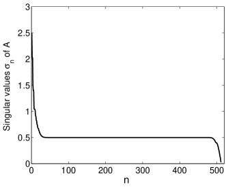
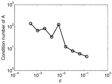
Figure 1: The first graph shows the singular values of $A$ in the decreasing order ($n$) when $\epsilon$ is 0.0020. The second graph shows the condition numbers of $A$ as $\epsilon$ tends to $0$ (from right to left). We use 256 grid points on each $B_{i}$, $i=1,2$, and hence the dimension of $A$ is $512\times 512$.

5.1 Computation for the perfectly conducting case

In this subsection we present a new method of computing the solution to (2.4) based on the characterization of the singular terms obtained in this paper.

Let

$$\tilde{h}({\bf x}) =h({\bf x})-\frac{1}{2\pi}\bigr{(}\log|{\bf x}-{\bf c}_{1}|-\log|{\bf x}-{\bf c}_{2}|\bigr{)}$$

$$=\frac{1}{2\pi}\bigr{(}\log|{\bf x}-{\bf p}_{1}|-\log|{\bf x}-{\bf p}_{2}|-\log|{\bf x}-{\bf c}_{1}|+\log|{\bf x}-{\bf c}_{2}|\bigr{)}$$ (5.5)

for ${\bf x}\in\mathbb{R}^{2}\setminus(B_{1}\cup B_{2})$. This modified function has the property that $\int_{\partial B_{i}}\tilde{h}=0$ for $i=1,2$, which is useful for the computation.

In view of (2.10), we look for a solution in the following form

$$u({\bf x})=a\tilde{h}({\bf x})+H({\bf x})+\mathcal{S}_{B_{1}}[\psi_{1}]({\bf x})+\mathcal{S}_{B_{2}}[\psi_{2}]({\bf x}),\qquad{\bf x}\in\mathbb{R}^{2}\setminus(B_{1}\cup B_{2}),$$ (5.6)

instead of (5.1), where $a$ is given by (2.11). According to Theorem 2.1, the gradient of the function $H+\mathcal{S}_{B_{1}}[\psi_{1}]+\mathcal{S}_{B_{2}}[\psi_{2}]$ is bounded on $\Omega\setminus(B_{1}\cup B_{2})$ for some bounded set $\Omega$ containing $B_{1}\cup B_{2}$, and hence $\|\psi_{1}\|_{L^{\infty}(\partial B_{1})}$ and $\|\psi_{2}\|_{L^{\infty}(\partial B_{2})}$ are bounded regardless of $\epsilon$.

To find the integral equation for density functions $(\psi_{1},\psi_{2})$, we argue as follows: Let $\tilde{h}^{e}$ be the extension of $\tilde{h}$ defined by $\tilde{h}^{e}({\bf x})=\tilde{h}({\bf x})$ for ${\bf x}\in\mathbb{R}^{2}\setminus(B_{1}\cup B_{2})$ and

$$\tilde{h}^{e}({\bf x})=\begin{cases}\displaystyle h|_{\partial B_{1}}-\frac{\log r_{1}}{2\pi}+\frac{1}{2\pi}\log|{\bf x}-{\bf c}_{2}|,\quad{\bf x}\in B_{1},\\ \vskip 6.0pt plus 2.0pt minus 2.0pt\cr\displaystyle h|_{\partial B_{2}}+\frac{\log r_{2}}{2\pi}-\frac{1}{2\pi}\log|{\bf x}-{\bf c}_{1}|,\quad{\bf x}\in B_{2}.\end{cases}$$ (5.7)

Then $\tilde{h}^{e}=\tilde{h}$ on $\partial B_{i}$ for $i=1,2$, and $\tilde{h}^{e}$ is harmonic in $B_{1}$ and $B_{2}$ as well as in $\mathbb{R}^{2}\setminus\overline{B_{1}\cup B_{2}}$. Define

$$u^{e}({\bf x})=a\tilde{h}^{e}({\bf x})+H({\bf x})+\mathcal{S}_{B_{1}}[\psi_{1}]({\bf x})+\mathcal{S}_{B_{2}}[\psi_{2}]({\bf x}),\qquad{\bf x}\in\mathbb{R}^{2}.$$

Then $u^{e}$ is continuous in $\mathbb{R}^{2}$ and harmonic in $B_{1}\cup B_{2}$. Since $u^{e}=u$ is constant on $\partial B_{i}$, $i=1,2$, $u^{e}$ is constant in $B_{i}$, $i=1,2$. By taking the interior normal derivative of $u^{e}$, one can see that $(\psi_{1},\psi_{2})\in L^{2}_{0}(\partial B_{1})\times L^{2}_{0}(\partial B_{2})$ is the unique solution to

$$\left\{\begin{array}[]{l}\displaystyle\frac{1}{2}\psi_{1}+\frac{\partial(\mathcal{S}_{B_{2}}[\psi_{2}])}{\partial\nu^{(1)}}=-\frac{\partial H}{\partial\nu^{(1)}}-a\frac{\partial\tilde{h}^{e}}{\partial\nu^{(1)}}\bigr{|}_{-}\quad\mbox{on }\partial B_{1},\\ \vskip 6.0pt plus 2.0pt minus 2.0pt\cr\displaystyle\frac{\partial(\mathcal{S}_{B_{1}}[\psi_{1}])}{\partial\nu^{(2)}}+\frac{1}{2}\psi_{2}=-\frac{\partial H}{\partial\nu^{(2)}}-a\frac{\partial\tilde{h}^{e}}{\partial\nu^{(2)}}\bigr{|}_{-}\quad\mbox{on }\partial B_{2}.\end{array}\right.$$ (5.8)

Moreover, we have from (5.7)

$$\frac{\partial\tilde{h}^{e}}{\partial\nu^{(1)}}\bigr{|}_{-}({\bf x}) =\frac{1}{2\pi}\frac{\langle{\bf x}-{\bf c}_{2},\nu^{(1)}({\bf x})\rangle}{|{\bf x}-{\bf c}_{2}|^{2}},\quad{\bf x}\in\partial B_{1},$$

$$\frac{\partial\tilde{h}^{e}}{\partial\nu^{(2)}}\bigr{|}_{-}({\bf x}) =-\frac{1}{2\pi}\frac{\langle{\bf x}-{\bf c}_{1},\nu^{(2)}({\bf x})\rangle}{|{\bf x}-{\bf c}_{1}|^{2}},\quad{\bf x}\in\partial B_{2}.$$

We can discretize (5.8) and solve (5.4) to obtain $(\psi_{1},\psi_{2})$. Here $Y_{1}$ and $Y_{2}$ are given by

$$Y_{1}=\begin{bmatrix}-\frac{\partial H}{\partial\nu^{(1)}}({\bf x}_{1}^{1})-\frac{a}{2\pi}\frac{\langle{\bf x}_{1}^{1}-{\bf c}_{2},\ \nu^{(1)}({\bf x}_{1}^{1})\rangle}{|{\bf x}_{1}^{1}-{\bf c}_{2}|^{2}}\\ \vdots\\ -\frac{\partial H}{\partial\nu^{(1)}}({\bf x}_{1}^{M})-\frac{a}{2\pi}\frac{\langle{\bf x}_{1}^{M}-{\bf c}_{2},\ \nu^{(1)}({\bf x}_{1}^{M})\rangle}{|{\bf x}_{1}^{M}-{\bf c}_{2}|^{2}}\end{bmatrix},\quad Y_{2}=\begin{bmatrix}-\frac{\partial H}{\partial\nu^{(2)}}({\bf x}_{2}^{1})+\frac{a}{2\pi}\frac{\langle{\bf x}_{2}^{1}-{\bf c}_{1},\ \nu^{(2)}({\bf x}_{2}^{1})\rangle}{|{\bf x}_{2}^{1}-{\bf c}_{1}|^{2}}\\ \vdots\\ -\frac{\partial H}{\partial\nu^{(2)}}({\bf x}_{2}^{M})+\frac{a}{2\pi}\frac{\langle{\bf x}_{2}^{M}-{\bf c}_{1},\ \nu^{(2)}({\bf x}_{2}^{M})\rangle}{|{\bf x}_{2}^{M}-{\bf c}_{1}|^{2}}\end{bmatrix}.$$ (5.9)

While $(\varphi_{1},\varphi_{2})$ in the representation (5.1) increases arbitrarily as $\epsilon$ tends to 0, $(\psi_{1},\psi_{2})$ stays bounded. The difference between the actual $(\psi_{1},\psi_{2})$ and the numerically obtained one is much smaller than that for $(\varphi_{1},\varphi_{2})$ as Figure 3 shows.

The first graph of Figure 2 shows the inner products of $Y$ in (5.4) with singular vectors of $A$ corresponding to small singular values. The dotted graph is when (5.3) is used and solid one is when (5.9) is used. The inner product using (5.3) is larger than the one using (5.9). This is expected: since the difference between the single layer potential and its discretization is large in the narrow region between two disks, the singular vector (corresponding to small singular values) components of this difference is not small. The second graph in Figure 2 shows the inner products of $A\begin{bmatrix}\varphi_{1}\\ \varphi_{2}\end{bmatrix}-Y$ with singular vectors of $A$ corresponding to small singular values, where $(\varphi,\varphi_{2})$ is the (numerical) solution to (5.4) using $Y$ in (5.3) (dotted line) and in (5.9) (solid line). This numerical solution is obtained using the method described in subsection 5.3 (with high precision). The graphs clearly show that the method of this paper works much better than the standard method. Here $H({\bf x})=x_{1}$.

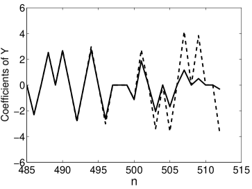
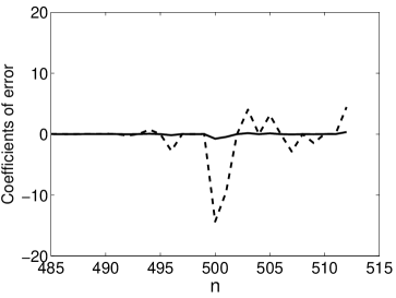
Figure 2: The first graph shows the inner product of singular vectors (corresponding small singular values) of $A$ with $Y$ in (5.4), where $Y$ is the discretization of the right hand side of (3.8) (the dashed line), and of (5.8) (the solid line). The second graph shows the inner product of singular vectors (corresponding small singular values) of $A$ with the error in (5.4). The radii of disks are fixed as $r_{1}=r_{2}=1$, and the number of equi-spaced grid points is 256 on each $\partial B_{i}$. The distance $\epsilon=0.0020$, and the background potential is given by $H({\bf x})=x_{1}$. $n$ indicates the location of singular values when listed in decreasing order.

5.2 Computation for the insulated case

Let $h_{\bot}$ be the function defined by (4.4). Since $\arg({\bf x}-{\bf p}_{1})-\arg({\bf x}-{\bf p}_{2})-\arg({\bf x}-{\bf c}_{1})$ is a harmonic conjugate of $\log|{\bf x}-{\bf p}_{1}|-\log|{\bf x}-{\bf p}_{2}|-\log|{\bf x}-{\bf c}_{1}|$, which is constant on $\partial B_{1}$, we have

$$\frac{\partial}{\partial\nu}\bigr{(}\arg({\bf x}-{\bf p}_{1})-\arg({\bf x}-{\bf p}_{2})-\arg({\bf x}-{\bf c}_{1})\bigr{)}=0,\quad\mbox{on }\partial B_{1}.$$

Hence,

$$\frac{\partial h_{\bot}}{\partial\nu^{(1)}}({\bf x})=\frac{1}{2\pi}\frac{\partial(\arg({\bf x}-{\bf c}_{2}))}{\partial\nu^{(1)}}\Bigr{|}_{\partial B_{1}}=\frac{1}{2\pi}\frac{\langle({\bf x}-{\bf c}_{2})^{\perp},\nu^{(1)}({\bf x})\rangle}{|{\bf x}-{\bf c}_{2}|^{2}},\quad{\bf x}\in\partial B_{1}.$$ (5.10)

Similarly, we have

$$\frac{\partial h_{\bot}}{\partial\nu^{(2)}}({\bf x})=-\frac{1}{2\pi}\frac{\partial(\arg({\bf x}-{\bf c}_{1}))}{\partial\nu^{(2)}}\Bigr{|}_{\partial B_{2}}=-\frac{1}{2\pi}\frac{\langle({\bf x}-{\bf c}_{1})^{\perp},\nu^{(2)}({\bf x})\rangle}{|{\bf x}-{\bf c}_{1}|^{2}},\quad{\bf x}\in\partial B_{2}.$$ (5.11)

We look for a solution $u$ to (4.1) in the following form:

$$u({\bf x})=a_{\bot}h_{\bot}({\bf x})+H({\bf x})+\mathcal{S}_{B_{1}}[\psi_{1}]({\bf x})+\mathcal{S}_{B_{2}}[\psi_{2}]({\bf x}),\qquad x\in\mathbb{R}^{2}\setminus(B_{1}\cup B_{2}),$$ (5.12)

where $a_{\bot}$ is given by (4.7) and $(\psi_{1},\psi_{2})\in L^{2}_{0}(\partial B_{1})\times L^{2}_{0}(\partial B_{2})$ is the solution to

$$\left\{\begin{array}[]{l}\displaystyle\frac{1}{2}\psi_{1}-\frac{\partial(\mathcal{S}_{B_{2}}[\psi_{2}])}{\partial\nu^{(1)}}=\frac{\partial H}{\partial\nu^{(1)}}+\frac{a}{2\pi}\frac{\langle({\bf x}-{\bf c}_{2})^{\perp},\nu^{(1)}({\bf x})\rangle}{|{\bf x}-{\bf c}_{2}|^{2}}\quad\mbox{on }\partial B_{1},\\ \vskip 6.0pt plus 2.0pt minus 2.0pt\cr\displaystyle-\frac{\partial(\mathcal{S}_{B_{1}}[\psi_{1}])}{\partial\nu^{(2)}}+\frac{1}{2}\psi_{2}=\frac{\partial H}{\partial\nu^{(2)}}-\frac{a}{2\pi}\frac{\langle({\bf x}-{\bf c}_{1})^{\perp},\nu^{(2)}({\bf x})\rangle}{|{\bf x}-{\bf c}_{1}|^{2}}\quad\mbox{on }\partial B_{2}.\end{array}\right.$$ (5.13)

5.3 Numerical Illustration

In this subsection, we illustrate results of numerical computations using the algorithms proposed in the previous subsections. Two discs are $B_{j}=B({\bf c}_{j},r_{j})$, $j=1,2$, of radius $r_{j}$ and centered at ${\bf c}_{1}=(-r_{1}-\epsilon/2,0)$ and ${\bf c}_{2}=(r_{2}+\epsilon/2,0)$.

We compute the solution in two different ways and compare them to demonstrate the effectiveness of the method proposed in this paper. We first compute the solution using the standard representation of the solution, namely, we use (5.1) and solve numerically (3.8). The discretization for the computation was described at the beginning of this section. We denote by $u$ the solution computed by this method. We then compute the solution using the representation (5.6) and solve (5.8). The solution is denoted by $u^{h}$. For comparison we solve (5.8) yet another method which provides the solution with higher precision (but with high cost).

Let $R_{i}$, $i=1,2$, be the reflection with respect to the disks $B_{i}$ defined by (2.6). We also define the the reflection of a function $f$ by $(R_{i}f)({\bf x})=f(R_{i}({\bf x}))$ for ${\bf x}\in\mathbb{R}^{2}$. Using the same argument as in [3] (see also [11]), one can show that the solution $(\psi_{1},\psi_{2})$ to (5.8) is given by

$$\psi_{1}=-2\sum_{m=0}^{\infty}\frac{\partial}{\partial\nu^{(1)}}\bigg{[}(R_{2}R_{1})^{m}\Bigr{(}H+\frac{a}{2\pi}\log|{\bf x}-{\bf c}_{2}|-R_{2}\bigr{[}H-\frac{a}{2\pi}\log|{\bf x}-{\bf c}_{1}|\bigr{]}\Bigr{)}\bigg{]}\Bigr{|}_{\partial B_{1}},$$

$$\psi_{2}=-2\sum_{m=0}^{\infty}\frac{\partial}{\partial\nu^{(2)}}\bigg{[}(R_{1}R_{2})^{m}(H-\frac{a}{2\pi}\log|{\bf x}-{\bf c}_{1}|-R_{1}\bigr{[}H+\frac{a}{2\pi}\log|{\bf x}-{\bf c}_{2}|\bigr{]}\Bigr{)}\bigg{]}\Bigr{|}_{\partial B_{2}}.$$

We denote by $u^{R}$ the solution obtained by this method. We compare these solutions for various values of $\epsilon$. The radii are fixed as $r_{1}=2$ and $r_{2}=1.5$, and the number of equi-spaced grid points is 256 on each $\partial B_{i}$. The background potential is given by $H({\bf x})=2x_{1}+(x_{1}^{2}-x_{2}^{2})$. Figure 3 shows the relative $L^{2}$-errors of the normal flux $\frac{\partial u}{\partial\nu}$ and $\frac{\partial u^{h}}{\partial\nu}$, compared to the normal flux $\frac{\partial u^{R}}{\partial\nu}$. The vertical axis in the figure represents the values of

$$\frac{\left\|\frac{\partial u^{h}}{\partial\nu^{(1)}}-\frac{\partial u^{R}}{\partial\nu^{(1)}}\right\|_{L^{2}(\partial B_{1})}}{2\left\|\frac{\partial u^{R}}{\partial\nu^{(1)}}\right\|_{L^{2}(\partial B_{1})}}+\frac{\left\|\frac{\partial u^{h}}{\partial\nu^{(2)}}-\frac{\partial u^{R}}{\partial\nu^{(2)}}\right\|_{L^{2}(\partial B_{2})}}{2\left\|\frac{\partial u^{R}}{\partial\nu^{(2)}}\right\|_{L^{2}(\partial B_{2})}}$$

indicated by circles and

$$\frac{\left\|\frac{\partial u}{\partial\nu^{(1)}}-\frac{\partial u^{R}}{\partial\nu^{(1)}}\right\|_{L^{2}(\partial B_{1})}}{2\left\|\frac{\partial u^{R}}{\partial\nu^{(1)}}\right\|_{L^{2}(\partial B_{1})}}+\frac{\left\|\frac{\partial u}{\partial\nu^{(2)}}-\frac{\partial u^{R}}{\partial\nu^{(2)}}\right\|_{L^{2}(\partial B_{2})}}{2\left\|\frac{\partial u^{R}}{\partial\nu^{(2)}}\right\|_{L^{2}(\partial B_{2})}}$$

indicated by squares. As $\epsilon$ decreases (from right to left), the relative error increases for $u$ and $u^{h}$ as expected. However, the relative error of $u^{h}$ is notably small compared to that of $u$: when $\epsilon\sim 0.001$, the relative error of $u^{h}$ is as small as 0.01, but that of $u$ is as big as 1.

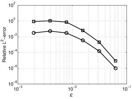
Figure 3: The circles are the relative errors of $\frac{\partial u^{h}}{\partial\nu}$ compared to $\frac{\partial u^{R}}{\partial\nu}$, and the squares are those of $\frac{\partial u}{\partial\nu}$. Both depend on the distance $\epsilon$ between two perfectly conducting disks. The solution based on the asymptotic expansion has much smaller error. We use 256 grid points on each $B_{i}$, $i=1,2$.

In Figure 4, fixing $\epsilon=0.0156$, we compare the relative errors for different grid numbers. Both radii are 1, and $H({\bf x})=x_{1}$. The difference between the normal flux $\frac{\partial u}{\partial\nu^{(j)}}$ and $\frac{\partial u^{R}}{\partial\nu^{(j)}}$ takes its maximum value at the point nearest the middle point of the shortest line segment between $\partial B_{1}$ and $\partial B_{2}$, which is the same for $\frac{\partial u^{h}}{\partial\nu^{(j)}}$. As the grid numbers increase, both the relative $L^{2}$-error and the maximal difference decrease. But, relative errors of $u^{h}$ are much smaller than those of $u$.

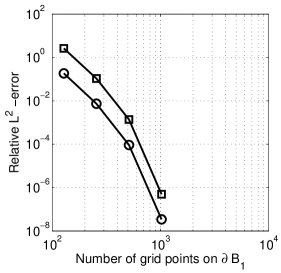
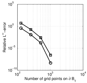
Figure 4: The circles are the relative errors of $\frac{\partial u^{h}}{\partial\nu}$ compared to $\frac{\partial u^{R}}{\partial\nu}$, and the squares are those of $\frac{\partial u^{h}}{\partial\nu}$ in $L^{2}$ and $L^{\infty}$ norms for various grid numbers. The solution based on the asymptotic expansion has much smaller error.

In Figure 5 and 6, the uniformly spaced contour level curves are drawn for the free space conducting and insulating case, respectively. The distance $\epsilon=0.0156$ and the number of grid points on each disk is 256. The radii are $r_{1}=r_{2}=1$ except the lower-right figure where $r_{2}=2$. The entire harmonic function $H({\bf x})=x_{1}$ in the upper-left and the lower-right figure, and $H({\bf x})=x_{2}$ in the upper-right one, and $H({\bf x})=x_{1}-x_{2}$ in the lower-left one.

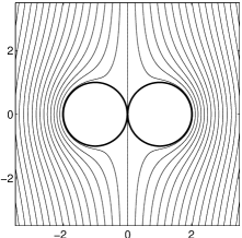
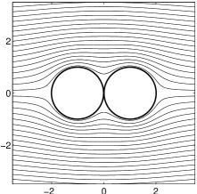
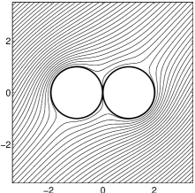
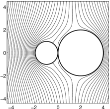
Figure 5: Level curves of the free space conducting case. The entire harmonic function $H({\bf x})=x_{1}$ in the upper-left and the lower-right figure, and $H({\bf x})=x_{2}$ in the upper-right one, and $H({\bf x})=x_{1}-x_{2}$ in the lower-left one.

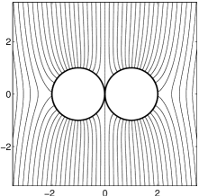
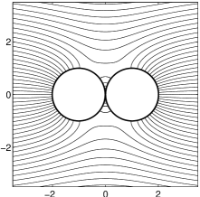
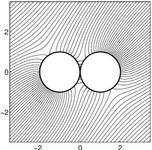
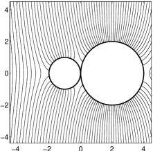
Figure 6: Level curves of the free space insulating case. The entire harmonic function $H({\bf x})=x_{1}$ in the upper-left and the lower-right figure, and $H({\bf x})=x_{2}$ in the upper-right one, and $H({\bf x})=x_{1}-x_{2}$ in the lower-left one.

References

[1] H. Ammari, G. Dassios, H. Kang H and M. Lim, Estimates for the electric field in the presence of adjacent perfectly conducting spheres, Quat. Appl. Math. 65 (2007), 339–355.
[2] H. Ammari and H. Kang, Polarization and moment
tensors with applications to inverse problems and effective medium
theory, Applied Mathematical Sciences, Vol. 162, Springer-Verlag,
New York, 2007.
[3] H. Ammari, H. Kang and M. Lim, Gradient estimates for solutions to the conductivity problem, Math. Ann. 332(2) (2005), 277–286.
[4] H. Ammari, H. Kang, H. Lee, J. Lee and M. Lim, Optimal bounds on the gradient of solutions to conductivity problems, J. Math. Pures Appl. 88 (2007), 307–324.
[5] H. Ammari, H. Kang, H. Lee, M. Lim and H. Zribi, Decomposition theorems and fine estimates for electrical fields in the presence of closely located circular inclusions, Jour. Diff. Equa., 247 (2009), 2897-2912.
[6] I. Babus̆ka, B. Andersson, P. Smith and K. Levin, Damage analysis of fiber composites. I. Statistical
analysis on fiber scale, Comput. Methods Appl. Mech. Engrg. 172 (1999), 27–77.
[7] B. Budiansky and G. F. Carrier, High shear stresses in stiff fiber composites, Jour. Appl. Mech. 51 (1984), 733-735.
[8] E. S. Bao, Y.Y. Li and B. Yin, Gradient estimates for the perfect conductivity problem, Arch. Rat. Mech. Anal. 193 (2009), 195-226.
[9] E. S. Bao, Y.Y. Li and B. Yin, Gradient Estimates for the perfect and insulated conductivity problems with multiple inclusions, Comm. Part. Diff. Equa. 35 (2010), 1982–2006.
[10] E. Bonnetier and M. Vogelius, An elliptic regularity result for a composite medium with “touching” fibers of circular cross-section, SIAM Jour. Math. Anal. 31 No 3 (2000), 651–677.
[11] H. Cheng and L. Greengard,
A method of images for the evaluation of electrostatic
fields in systems of closely spaced conducting cylinders,
SIAM J. Appl. Math. 58 (1998), 122-141.
[12] L. Greengard and M. Moura,
On the numerical evaluation of electrostatic fields in
composite materials,
Acta Numerica (1994), 379–410.
[13] E. Fabes, H. Kang, and J.K. Seo, Inverse conductivity problem
with one measurement: Error estimates and approximate
identification for perturbed disks,
SIAM J. Math. Anal., 30 (1999), 699–720.
[14] H. Kang and J.K. Seo, Layer potential technique for the inverse
conductivity problem, Inverse Problems, 12 (1996), 267–278.
[15]
H. Kang and J.K. Seo, Recent progress in the inverse conductivity problem with
single measurement, in Inverse Problems and Related Fields, CRC
Press, Boca Raton, FL, (2000), 69–80.
[16] J.B. Keller, Stresses in narrow regions, Trans. ASME J. Appl. Mech. 60 (1993), 1054–1056.
[17] X. Markenscoff, Stress amplification in vanishing
small geometries, Computational Mechanics 19 (1996), 77–83.
[18] Y.Y. Li and L. Nirenberg, Estimates for elliptic system from composite material, Comm. Pure Appl. Math., LVI (2003), 892–925.
[19] Y.Y. Li and M. Vogelius, Gradient estimates for solution to divergence form elliptic equation with discontinuous coefficients, Arch. Rat. Mech. Anal. 153 (2000), 91–151.
[20] M. Lim and K. Yun, Blow-up of electric fields between closely spaced spherical perfect conductors, Comm. Part. Diff. Equa. 34 (2009), 1287–1315.
[21] M. Lim and K. Yun, Strong influence of a small fiber on shear stress in fiber-reinforced composites, Jour. Diff. Equa. 250 (2011), 2402–2439.
[22] K. Yun, Estimates for electric fields blown up between closely adjacent conductors with arbitrary shape, SIAM Jour. Appl. Math. 67 No 3 (2007), 714–730.
[23] K. Yun, Optimal bound on high stresses occurring between stiff fibers with arbitrary shaped cross sections, Jour. Math. Anal. Appl. 350 (2009), 306-312.