Stochastic population oscillations in spatial predator-prey models

Abstract

It is well-established that including spatial structure and stochastic noise in models for predator-prey interactions invalidates the classical deterministic Lotka–Volterra picture of neutral population cycles. In contrast, stochastic models yield long-lived, but ultimately decaying erratic population oscillations, which can be understood through a resonant amplification mechanism for density fluctuations. In Monte Carlo simulations of spatial stochastic predator-prey systems, one observes striking complex spatio-temporal structures. These spreading activity fronts induce persistent correlations between predators and prey. In the presence of local particle density restrictions (finite prey carrying capacity), there exists an extinction threshold for the predator population. The accompanying continuous non-equilibrium phase transition is governed by the directed-percolation universality class. We employ field-theoretic methods based on the Doi–Peliti representation of the master equation for stochastic particle interaction models to (i) map the ensuing action in the vicinity of the absorbing state phase transition to Reggeon field theory, and (ii) to quantitatively address fluctuation-induced renormalizations of the population oscillation frequency, damping, and diffusion coefficients in the species coexistence phase.

1 Introduction

Over the past decade, mathematical and computational tools from statistical physics have been increasingly and quite successfully applied to ecological problems, including attempts at a quantitative understanding of biodiversity [1]–[4]. In this context, physicists typically consider simplified idealized models that hopefully capture the essential features of interacting biosystems; leaving aside some of the biological complexity allows the consistent incorporation of stochastic fluctuations and spatio-temporal correlations, whose crucial importance has long been recognized in the field [5], but is still often neglected.

Predator-prey models defined via reaction-diffusion systems on a regular lattice, whose rate equations in the well-mixed mean-field limit reduce to the classic coupled Lotka–Volterra ordinary differential equations, constitute paradigmatic examples of the dynamics of two competing populations [6]–[8]. Monte Carlo simulations of these models, specifically in two dimensions, display a remarkable wealth of intriguing features (for a fairly recent overview, see, e.g., Ref. [9]): In contrast to the regular non-linear oscillations of the deterministic Lotka–Volterra model for which the population densities invariably return to their initial values (c.f. figure 1 below), computer simulations display persistent, but eventually decaying stochastic population oscillations (figure 2) [10]–[17]. In the absence of spatial degrees of freedom, these erratic population oscillations may be understood through a resonant stochastic amplification mechanism [18] that drastically extends the transient time interval before any finite system ultimately reaches its absorbing stationary state, where the predator population becomes extinct [19]. In spatially extended systems, it is well-known that the mean-field Lotka–Volterra reaction-diffusion equations allow for traveling wave solutions [20]–[22]. In the corresponding stochastic spatial realizations, spreading activity fronts (figure 4, [23]) induce short-ranged but significant positive correlations of either species, and anti-correlations between the predator and prey populations, which have the effect of further enhancing the amplitude and life time of local population oscillations [9, 24]. We have investigated various different variants of stochastic spatial Lotka–Volterra models for competing predator-prey populations, and found these intriguing spatio-temporal structures to be remarkably robust against rather drastic changes of the detailed microscopic interaction rules [24, 25], and even the introduction of quenched spatial disorder in the reaction rates [26].

In this brief communication, I will provide an overview of our Monte Carlo simulation results, specifically contrasting model variants with and without restrictions on the number of particles per lattice site. The former describe ecological systems with finite local carrying capacity, and display a continuous non-equilibrium phase transition from an active species coexistence state to an absorbing phase wherein the predators become extinct. Numerical evidence supports the general expectation [27]–[32] that this extinction transition should be governed by the directed-percolation universality class [7, 8], [11]–[14], [16, 17]. I will then demonstrate how field-theoretic tools based on the Doi–Peliti representation of the master equation for stochastic interacting particle systems [33]–[35] (for recent reviews, see Refs. [36, 37]), augmented with a means to incorporate restricted site occupation numbers [38], can be employed to gain a comprehensive understanding of fluctuation and correlation effects in Lotka–Volterra predator models. Specifically, the effective action near the extinction transition in model variants with restricted site occupations will be explicitly mapped onto Reggeon field theory which describes the universal scaling of directed-percolation clusters [27, 32, 39, 40]. Moreover, expanding on the treatment in Ref. [41], I shall report a computation of the fluctuation-induced renormalizations of the population oscillation frequency, damping, and diffusion coefficients in the species coexistence phase to lowest order in a perturbation expansion with respect to the predation rate [42].

2 Stochastic lattice Lotka–Volterra models

2.1 Model variants and mean-field description

We consider a two-species system of diffusing particles (with diffusion constant $D$) that undergo the following stochastic reactions:

$$A\to\emptyset\quad {\rm with\ rate}\ \mu,$$

$$A+B\to A+A\quad {\rm with\ rate}\ \lambda,$$

$$B\to B+B\quad {\rm with\ rate}\ \sigma.$$

The ‘predators’ $A$ decay or die spontaneously at rate $\mu>0$, whereas the ‘prey’ $B$ produce offspring with rate $\sigma>0$. In the absence of the binary ‘predation’ interaction with rate $\lambda$, the uncoupled first-order processes would naturally lead to predator extinction $a(t)=a(0)\,e^{-\mu t}$, and Malthusian prey population explosion $b(t)=b(0)\,e^{\sigma t}$; here $a(t)$ and $b(t)$ respectively indicate the $A$ / $B$ concentrations or population densities. The binary predation reaction induces species coexistence through the non-linear interaction of both particle species.

In the simplest spatial realization of this stochastic reaction-diffusion model, both particle species are represented by unbiased random walkers on a $d$-dimensional hypercubic lattice, and we allow an arbitrary number of particles per lattice site [24]. All reactions (2.1) can then be implemented strictly on-site: Offspring particles are placed on the same lattice point as their parents, and the predation reaction happens only if an $A$ and a $B$ particle meet on the same lattice site. If we then assume the populations to remain well mixed, and consequently ignore both spatial fluctuations and correlations, we can approximately describe the coupled reactions (2.1) through the associated mean-field rate equations for spatially homogeneous concentrations $a(t)=\langle a({\vec{x}},t)\rangle$, $b(t)=\langle b({\vec{x}},t)\rangle$, where $a({\vec{x}},t)$ and $b({\vec{x}},t)$ respectively denote the local predator and prey densities. One then arrives at the classic Lotka–Volterra equations [4], a coupled set of two ordinary non-linear differential equations:

$$\dot{a}(t)=\lambda\,a(t)\,b(t)-\mu\,a(t)\ ,\quad\dot{b}(t)=\sigma\,b(t)-\lambda\,a(t)\,b(t)\ .$$ (2)

The rate equations (2) display three stationary states $(a_{s},b_{s})$, namely the empty absorbing state with total population extinction $(0,0)$, which is obviously linearly unstable if $\sigma>0$; a predator extinction absorbing state wherein the prey population diverges $(0,\infty)$, which for $\lambda>0$ is also linearly unstable; and finally a species coexistence state $(a_{u}=\sigma/\lambda,b_{u}=\mu/\lambda)$, which however represents only a marginally stable fixed point with purely imaginary eigenvalues $\pm i\sqrt{\mu\,\sigma}$ of the associated Jacobian stability matrix: Linearizing eqs. (2) near $(a_{u},b_{u})$ results in the coupled differential equations $\delta\dot{a}(t)=\sigma\,\delta b(t)$, $\delta\dot{b}(t)=-\mu\,\delta a(t)$, which are readily solved by $\delta a(t)=\delta a(0)\,\cos\left(\sqrt{\mu\,\sigma}\,t\right)+\delta b(0)\,\sqrt{\sigma/\mu}\,\sin\left(\sqrt{\mu\,\sigma}\,t\right)$ and $\delta b(t)=-\delta a(0)\,\sqrt{\mu/\sigma}\,\sin\left(\sqrt{\mu\,\sigma}\,t\right)+\delta b(0)\,\cos\left(\sqrt{\mu\,\sigma}\,t\right)$, describing harmonic oscillations about the center fixed point $(a_{u},b_{u})$ with frequency $\omega=2\pi\,f=\sqrt{\mu\,\sigma}$. Indeed, the phase space trajectories for the full non-linear coupled differential equations (2) are determined by $da/db=a\,(\lambda\,b-\mu)/b\,(\sigma-\lambda\,a)$, with a conserved first integral

$$K(t)=\lambda[a(t)+b(t)]-\sigma\ln a(t)-\mu\ln b(t)=K(0)\ .$$ (3)

Consequently, as depicted in figure 1, the solutions of the deterministic mean-field Lotka–Volterra model are closed orbits in phase space, i.e., regular periodic non-linear population oscillations whose amplitudes are fixed by the initial configuration. Naturally, the precise periodic return to the initial concentration values does not appear to be a very realistic feature. In addition, the neutral cycles of the coupled mean-field rate equation system (2) indicates that this deterministic mathematical model is fundamentally unstable with respect to slight modifications [4].

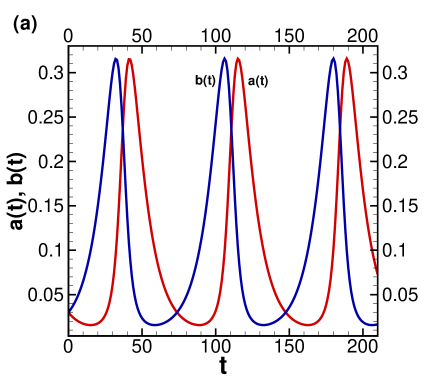
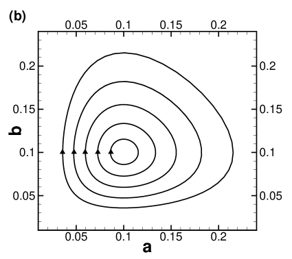
Figure 1: Solutions of the coupled Lotka–Volterra mean-field rate equations (2): (a) Non-linear predator $a(t)$ (red) and prey $b(t)$ (blue) population density oscillations; (b) periodic orbits in the $a$-$b$ phase plane. For small amplitudes the oscillations become harmonic (circular orbits) with frequency $\omega=\sqrt{\mu\,\sigma}$. (Reproduced with permission from Ref. [24], p. 4.)

One such modification that aims at rendering the Lotka–Volterra system more relevant biologically is to introduce a finite carrying capacity (total particle density) $\rho>0$ that limits the prey population growth, modeling, e.g., the effect of limited food resources [4]. Within the mean-field rate equation approximation, the second differential equation in (2) is then replaced with

$$\dot{b}(t)=\sigma\,b(t)\left[1-b(t)/\rho\right]-\lambda\,a(t)\,b(t)\ .$$ (4)

The non-trivial stationary states in this restricted Lotka–Volterra model are predator extinction and prey saturation $(0,\rho)$, linearly stable for $\lambda<\lambda_{c}=\mu/\rho$; and species coexistence $(a_{r},b_{r})$ with $b_{r}=\mu/\lambda$ and $a_{r}=(1-\mu/\rho\lambda)\sigma/\lambda$, which both exists and is linearly stable provided the predation rate is sufficiently large, $\lambda>\lambda_{c}$. The eigenvalues of the Jacobian now acquire negative real parts, $\epsilon_{\pm}=-\mu\,\sigma\left[1\pm\sqrt{1-4\rho\lambda\left(\rho\lambda/\mu-1\right)/\sigma}\right]/2\rho\lambda$, which implies an exponential approach to the stable fixed point $(a_{r},b_{r})$, replacing the neutral cycles of the unrestricted model (2). Moreover, for $\sigma>\sigma_{s}=4\lambda\,\rho\left(\rho\lambda/\mu-1\right)>0$, or $\mu/\rho<\lambda<\lambda_{s}=\left(1+\sqrt{1+\sigma/\mu}\right)\mu/2\rho$, the eigenvalues are real, indicating a nodal stable fixed point, whereas for $\sigma<\sigma_{s}$ or $\lambda>\lambda_{s}$, i.e., deep in the species coexistence phase, the eigenvalues $\epsilon_{\pm}$ turn into a complex conjugate pair, and $(a_{r},b_{r})$ becomes a stable spiral singularity which is approached in a damped oscillatory manner. Adding spatial degrees of freedom, finite local carrying capacities can be implemented in a lattice model through limiting the maximum occupation number per site for each species. Most drastically, one can permit at most a single particle per lattice site [9]; the binary predation reaction then has to occur between predators and prey on adjacent nearest-neighbor sites, and new offspring needs to be placed on neighboring positions. In that case, one can in fact entirely dispense with hopping processes, since all particle production reactions entail population spreading as well.

In summary, already within the mean-field rate approximation, a finite prey carrying capacity $\rho$, which can be viewed as the average result of local restrictions on the prey density originating from limited resources, crucially changes the phase diagram: There emerges an extinction threshold (at $\lambda_{c}$ for fixed $\mu$) for the predator population, which in a spatially extended system becomes a genuine continuous active-to-absorbing non-equilibrium phase transition in the thermodynamic limit of infinite system size and time.

2.2 Monte Carlo simulation results

Various authors have studied stochastic lattice predator-prey models that in the well-mixed mean-field limit reduce to the classical Lotka–Volterra system [6]–[8], [10]–[17]. In this section, I shall briefly discuss the pertinent results from our own individual-based Monte Carlo simulation studies, performed mostly on two-dimensional square lattices with periodic boundary conditions. Technical details and more precise descriptions of the algorithms we have employed can be found in Refs. [9] and [24].

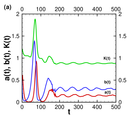
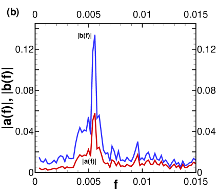
Figure 2: Monte Carlo simulation data for a stochastic spatial Lotka–Volterra system on a $1024\times 1024$ square lattice with periodic boundary conditions, in the absence of site occupation number restrictions: (a) Temporal evolution for the predator $a(t)$ (red) and prey $b(t)$ (blue) population densities, and the quantity $K(t)$ (green) for $\sigma=0.1$, $\mu=0.2,$, and $\lambda=1.0$; (b) Fourier-transformed population density signals $|a(f)|$ and $|b(f)|$ for $\sigma=0.03$, $\mu=0.1,$, and $\lambda=1.0$. (Reproduced with permission from Ref. [24], pp. 9 and 10.)

Figure 2 shows typical simulation data for the temporal evolution of the total predator and prey particle densities in a two-dimensional stochastic lattice model with (almost) arbitrarily large site occupation numbers and on-site reactions [24]. One observes long-lived but clearly damped population oscillations that are actually quite independent of the initial state; neither are they caused by the constancy of the first integral $K$, eq. (3), that follows from the deterministic rate equations: As is apparent from the numerical data, in the stochastic spatial model $K(t)$ is manifestly time-dependent, and in fact traces the overall population oscillations. We note that as the system size increases, the relative oscillation amplitudes become smaller; in the thermodynamic limit, the quasi-periodic population fluctuations eventually die out entirely. From the marked peaks in the Fourier-transformed concentration signals, $a(f)=\int a(t)\,e^{2\pi ift}\,dt$ for the predators, and similarly for the prey density, we may infer a characteristic oscillation frequency $f$. As illustrated in figure 3, the typical population oscillation frequencies thus obtained roughly follow the square-root dependence on the rates $\mu$ and $\sigma$ as predicted by the linearized mean-field approximation, but with measurable deviations both for low and high rates. Yet the numerical frequency values are reduced by about a factor of four in the stochastic spatially extended system, an apparent considerable downward renormalization caused by fluctuations and reaction-induced spatio-temporal correlations [24]. Note also that figure 3(a) shows a remarkably similar functional dependence of $f$ on the rates $\mu$ and $\sigma$.

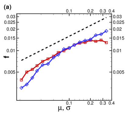
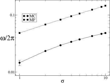
Figure 3: Characteristic peak frequencies obtained form $|a(f)|$ or $|b(f)|$, (a) as functions of the rates $\sigma$ (red squares) and $\mu$ (blue diamonds), with otherwise $\sigma=0.1=\mu$ and $\lambda=1.0$ held fixed on a $1024$ lattice without site occupation restrictions; (b) as function of $\sigma$ with $\mu=0.1$, $\lambda=1.6$, $D=0$ on a $128\times 128$ square lattice with at most a single particle per lattice site (black line). The dashed black lines represent the oscillation frequency from linearized mean-field theory, $f=\sqrt{\mu\,\sigma}$. (Reproduced with permission from Ref. [24], p. 10 and Ref. [9], p. 469.)

Very similar features are found in stochastic spatial Lotka–Volterra models that incorporate stringent site occupation number restrictions (allowing only at most one particle on each site), deep in the species coexistence phase, i.e., for large predation rates, corresponding to a stable focal mean-field fixed point (stability matrix eigenvalues with negative real and non-vanishing imaginary parts). Both in the absence and presence of local density limitations, the coexistence phase is governed by remarkably strong spatio-temporal fluctuations: Striking spreading activity waves of prey closely followed by predators periodically sweep the system; any small surviving clusters of prey subsequently serve as sources for resurgent expanding prey-predator fronts [9]. An average over these weakly coupled local oscillations then yields the total population time traces depicted in figure 2. These spreading activity fronts appear especially sharp for the site-restricted model variants, as displayed in figure 4, whereas in realizations with arbitrarily many particles per site, the fronts look more diffuse [23]. In either situation, one can employ stationary-state correlation functions to measure the spatial width $\sim 10\ldots 20$ lattice sites of the spreading activity regions. At roughly the same length scale, the cross-correlations of the $A$ and $B$ particles peak at a positive value before slowly decaying to zero; at shorter distances, the prey are naturally anti-correlated with the predators [9, 24].

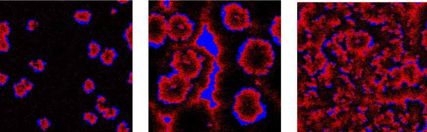
Figure 4: Snapshots illustrating the evolution in time (from left to right) of a two-dimensional stochastic lattice Lotka–Volterra model (with $512\times 512$ sites), incorporating local occupation number restrictions in the species coexistence phase, with rates $\sigma=4.0$, $\mu=0.1$, $\lambda=2.2$, and $D=0$, when the fixed point is a focus; the initial densities are $a(0)=1/3=b(0)$. The red, blue, and black dots respectively represent the prey, predators, and empty lattice sites. (Reproduced with permission from Ref. [9], p. 464.)

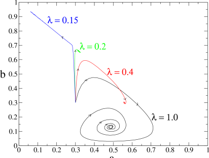
Figure 5: Typical trajectories in the predator-prey phase space for a $512\times 512$ stochastic lattice Lotka–Volterra system all initialized with $a(0)=1/3=b(0)$ and fixed rates $\sigma=4.0$, $\mu=0.1$, and $D=0$, but different predation rates $\lambda=0.15,0.20,0.40,1.0$. For small values of $\lambda$ (typically $\lambda<0.4$) the fixed point is a stable node, whereas for higher values of $\lambda$ one observe the characteristic spirals that indicate a focus in phase space. (Reproduced with permission from Ref. [9], p. 463.)

In the absence of spatial degrees of freedom, the observed persistent population oscillations can be mathematically understood by performing a systematic van-Kampen expansion about the absorbing steady state [18]. The fluctuation corrections may then essentially be described through a damped harmonic oscillator driven by white noise that will on occasion resonantly incite large-amplitude excursions away from the stable fixed point in the phase plane. In our spatial systems, we may also interpret the persistent population oscillations in the species coexistence regime through a similar mechanism, as suggested by the bottom spiraling trajectory (for large predation rate $\lambda=1.0$) in the phase portrait depicted in figure 5, which was obtained in simulation runs for stochastic lattice Lotka–Volterra models with restricted site occupancy [9]. As the rate $\lambda$ is reduced (with all other parameters held constant) and the predators become less efficient, the stochastic lattice systems with site occupation restrictions qualitatively display the same scenarios as revealed by the mean-field analysis for eqs. (4) with finite prey carrying capacity: First, the focal stationary points in the phase plane are replaced by stable nodes (real stability matrix eigenvalues); the population oscillations then cease, and no interesting spatial structures aside from localized activity clusters with meek fluctuations are seen (c.f. the trajectories for $\lambda=0.4$ and $0.2$ in figure 5). At a sufficiently small critical value $\lambda_{c}$ ($\approx 0.1688$ here, see figure 6), a predator extinction threshold is encountered, and for $\lambda<\lambda_{c}$ ultimately the prey population fills the entire lattice.

For the predator population, the extinction threshold in stochastic spatial Lotka–Volterra models with local particle density restrictions represents a genuine continuous non-equilibrium phase transition in the thermodynamic and infinite-time limit. Since no conserved quantities or disorder are present, one expects this active to absorbing state phase transition to be described by the scaling exponents of critical directed percolation [27]–[32]. Heuristically, one may reason as follows: The prey density is essentially uniform and constant $b\approx\rho$ near the critical point. The Lotka–Volterra reactions (2.1) then basically reduce to $A\to\emptyset$ and $A\to A+A$; but since the $A$ population cannot multiply to arbitrarily large density (due to prey depletion), we need to add a growth-limiting reaction such as $A+A\to A$, whereupon we arrive at the simplest microscopic reaction-diffusion model realization for the directed-percolation universality class [29, 31, 32, 37]. This assertion is indeed supported by careful analysis of Monte Carlo simulation data [7]–[9], [11]–[14], [16, 17]. We performed dynamical Monte Carlo simulations starting from a single active site with a predator particle in a lattice otherwise filled with prey, choosing reaction rates in the vicinity of the extinction threshold. The survival probability of predators at criticality is expected to decay algebraically as $P(t)\sim t^{-\delta^{\prime}}$, while the number of active sites with predators should grow according to the power law $N(t)\sim t^{\theta}$ [29, 31, 32], with $\delta^{\prime}\approx 0.451$ and $\theta\approx 0.230$ for directed percolation in two dimensions [29, 31]. Figure 6 shows the corresponding effective exponents as functions of inverse time as measured in our Monte Carlo simulations for various values of $\lambda$ with $\sigma=4.0$, $\mu=0.1$, and $D=0$ held fixed [9]. From these data we infer $\lambda_{c}\approx 0.1688$ as best estimate for the critical predation rate (compare with the mean-field prediction $\lambda_{c}=\mu=0.1$), and the extrapolation to $t\to\infty$ yields very good agreement of the asymptotic critical exponents with the accepted directed-percolation values.

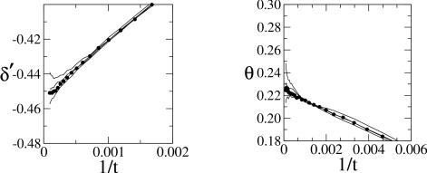
Figure 6: Dynamical Monte Carlo simulation data to estimate the critical point and scaling exponents for the predator extinction threshold of the two-dimensional stochastic lattice Lotka–Volterra model with site occupation restrictions (on a $512\times 512$ lattice): The effective scaling exponents $-\delta^{\prime}(t)$ vs. $1/t$ (left) and $\theta(t)$ vs. $1/t$ (right) are depicted for four values of $\lambda$ (from top to bottom): $0.1690$, $0.1689$, $0.1688$, and $0.1687$, at fixed $\sigma=4.0$, $\mu=0.1$, and $D=0$. (Reproduced with permission from Ref. [9], p. 470.)

Simulations in one spatial dimension (on a circular domain) yield remarkable differences between model variants with and without site occupation number restrictions: In the former situation, the $A$ and $B$ particles quickly segregate into distinct domains, with the predation reactions occurring only at the boundary. The subsequent time evolution is governed by very slow coarsening induced by merging predator domains [9]. Without site occupation restrictions, in contrast we always observe the active coexistence state [24]. All the above statements of course pertain to sufficiently large lattices. In principle, any finite system with an absorbing steady state will eventually terminate in it; however, the associated survival times are expected to grow with system size according to a power law [19], and for our lattices are much longer than the duration of the simulations.

3 Field-theoretic analysis

3.1 Field theory representation

In the remainder of this paper, I shall describe how stochastic fluctuations, internal reaction noise, and emerging correlations in spatial predator-prey models can be systematically captured by means of a field-theoretic representation of the associated classical master equation, which is then amenable to analytic approximations. Since the two-species Lotka–Volterra model (2.1) is defined via a diffusion-limited stochastic reaction system, we may employ the by now standard Doi–Peliti framework to map the associated master equation onto a field theory action [33]–[37]. This approach is based on the fact that at any time the configurations in such systems are completely enumerated through specifying the occupation numbers of each species per lattice site, and that all occurring stochastic processes merely modify these local integer occupation numbers. It is therefore natural to use bosonic creation and annihilation operators to formally represent the system’s temporal evolution which is given in terms of a stochastic master equation. Subsequently the continuum limit can be taken, which in the time domain is most conveniently accomplished through a coherent-state path integral representation for the evolution operator.

For the diffusion-limited reactions (2.1) in $d$ spatial dimensions one thus arrives at the following action [9] (see also Ref. [41])

$$S[{\hat{a}},a;{\hat{b}},b]=\int\!d^{d}x\int\!dt\,\biggl{[}\,{\hat{a}}\left(\partial_{t}-D_{A}\,\nabla^{2}\right)a+{\hat{b}}\left(\partial_{t}-D_{B}\,\nabla^{2}\right)b$$

$$\quad\qquad\qquad\qquad\qquad\ +\mu\left({\hat{a}}-1\right)a+\sigma\left(1-{\hat{b}}\right){\hat{b}}\,b+\lambda\left({\hat{b}}-{\hat{a}}\right){\hat{a}}\,a\,b\,\biggr{]}\,,$$ (5)

with $e^{-S}$ providing the statistical weight for any observables that must be functions of the local ‘density’ fields $a({\vec{x}},t)$ and $b({\vec{x}},t)$. The top line here obviously accounts for nearest-neighbor hopping processes in the continuum limit (through the inverse diffusion propagators with diffusivities $D_{A}$ and $D_{B}$ for the predators and prey, respectively). The bottom line in (5) contains the stochastic reactions: spontaneous predator death with rate $\mu$, prey birth with rate $\sigma$, and predation with rate $\lambda$. Note that each reaction process is represented by two contributions, originating from the gain and loss terms in the master equation. One can easily reconstruct these contributions in the action by noting that the second one directly reflects the reaction process itself through the annihilation operators $a$, $b$ and creation operators ${\hat{a}}$, ${\hat{b}}$, whereas the first one encodes the ‘order’ of the corresponding reaction (i.e., which powers of the concentrations ${\hat{a}}\,a$ and ${\hat{b}}\,b$ enter the rate equations). It is important to realize that the Doi–Peliti action faithfully contains all stochastic fluctuations associated with the underlying microscopic processes, namely discrete finite-number fluctuations and internal reaction noise [37]. Following van Wijland’s analysis [38], restricted site occupation numbers or finite local carrying capacities $\rho$ for the prey species can be incorporated in this bosonic formalism through the replacement $\sigma\to\sigma\,e^{-{\hat{b}}\,b/\rho}$ in the $B$ particle reproduction term. (Alternatively, a growth-limiting reaction such as $B+B\to B$ could have been added.)

The associated classical field equations follow from the stationarity conditions $\delta S/\delta a=0=\delta S/\delta b$, always solved by ${\hat{a}}=1={\hat{b}}$ (actually just reflecting probability conservation [37]), and $\delta S/\delta{\hat{a}}({\vec{x}},t)=0=\delta S/\delta{\hat{b}}({\vec{x}},t)$, which yields precisely the mean-field rate equations augmented by diffusion terms. Indeed, for $\rho=\infty$ one arrives at eqs. (2), while expanding to first order in $\rho^{-1}$ recovers eq. (4). It is then convenient to perform a field shift according to ${\hat{a}}=1+{\tilde{a}}$, ${\hat{b}}=1+{\tilde{b}}$, whereupon the action becomes, again to lowest order in the inverse carrying capacity,

$$S[{\tilde{a}},a;{\tilde{b}},b]=\int\!d^{d}x\int\!dt\,\biggl{[}\,{\tilde{a}}\left(\partial_{t}-D_{A}\,\nabla^{2}+\mu\right)a+{\tilde{b}}\left(\partial_{t}-D_{B}\,\nabla^{2}-\sigma\right)b$$

$$\quad\qquad\qquad\qquad\qquad\ -\sigma\,{\tilde{b}}^{2}\,b+\sigma\,\rho^{-1}\,(1+{\tilde{b}})^{2}\,{\tilde{b}}\,b^{2}-\lambda\,(1+{\tilde{a}})\,({\tilde{a}}-{\tilde{b}})\,a\,b\,\biggr{]}\,.$$ (6)

In the following, the ‘microscopic’ field theory action (6) will serve as the starting point (i) for further manipulations to identify the universality class of the continuous active to absorbing state phase transition at the predator extinction threshold, and (ii) to compute the fluctuation-induced renormalization to lowest order in the predation rate for the population oscillation frequency and damping, as well as the diffusion coefficient in the two-species coexistence phase.

3.2 Extinction transition and directed percolation

Our goal is to construct an effective field theory [9] that describes the universal scaling properties near the non-equilibrium phase transition at $\lambda_{c}\approx\mu/\rho$ where the predators go extinct, and the prey fill the entire lattice: $a_{s}=0$, $b_{s}\approx\rho$. Consequently we transform the action (6) to new fluctuating fields $c=b_{s}-b$ with $\langle c\rangle=0$, and ${\tilde{c}}=-{\tilde{b}}$:

$$S[{\tilde{a}},a;{\tilde{c}},c]=\int\!d^{d}x\int\!dt\,\biggl{[}\,{\tilde{a}}\left(\partial_{t}-D_{A}\,\nabla^{2}+\mu-\lambda\,b_{s}\right)a+{\tilde{c}}\left(\partial_{t}-D_{B}\nabla^{2}+(2b_{s}/\rho-1)\,\sigma\right)c$$

$$\quad\qquad\qquad\qquad\qquad\ +\sigma\,b_{s}(2b_{s}/\rho-1)\,{\tilde{c}}^{2}-\sigma\,\rho^{-1}\,b_{s}^{2}\,{\tilde{c}}^{3}-\sigma\,(4b_{s}/\rho-1)\,{\tilde{c}}^{2}\,c$$

$$\quad\qquad\qquad\qquad\qquad\ -\sigma\,\rho^{-1}\,(1+{\tilde{c}}^{2})\,{\tilde{c}}\,c^{2}+2\sigma\,\rho^{-1}\,{\tilde{c}}^{2}\,(c+b_{s}\,{\tilde{c}})\,c$$

$$\quad\qquad\qquad\qquad\qquad\ -\lambda\,b_{s}\left({\tilde{a}}^{2}+(1+{\tilde{a}})\,{\tilde{c}}\right)a+\lambda\left(1+{\tilde{a}}\right)\left({\tilde{a}}+{\tilde{c}}\right)a\,c\,\biggr{]}\,.$$ (7)

Next we note that the birth rate is a relevant parameter in the renormalization group sense, which scales to infinity under scale transformations; this observation simply expresses the fact that fluctuations of the nearly uniform prey population become strongly suppressed through the ‘mass’ term $\propto\sigma$ for the $c$ fields. It is therefore appropriate to introduce rescaled fields $\phi=\sqrt{\sigma}\,c$ and ${\tilde{\phi}}=\sqrt{\sigma}\,{\tilde{c}}$, and subsequently take the limit $\sigma\to\infty$, which yields the drastically reduced effective action

$$S_{\infty}[{\tilde{a}},a;{\tilde{\phi}},\phi]=\int\!d^{d}x\int\!dt\,\biggl{[}\,{\tilde{a}}\left(\partial_{t}-D_{A}\,\nabla^{2}+\mu-\lambda\,b_{s}\right)a-\lambda\,b_{s}\,{\tilde{a}}^{2}\,a+{\tilde{\phi}}\,\phi+b_{s}\,{\tilde{\phi}}^{2}\,\biggr{]}\,.$$ (8)

As a final step, one needs to add a growth-limiting process for the predator population, for example through the binary coagulation reaction $A+A\to A$ with rate $\tau$. Since the fields $\phi$ and ${\tilde{\phi}}$ only appear as a bilinear form in the action (8), they can readily be integrated out, leaving

$$S_{\infty}[{\widetilde{\psi}},\psi]=\int\!d^{d}x\int\!dt\,\Biggl{[}\,{\widetilde{\psi}}\biggl{(}\partial_{t}+D_{A}\,(r_{A}-\nabla^{2})\biggr{)}\psi-u\,{\widetilde{\psi}}\left({\widetilde{\psi}}-\psi\right)\psi+\tau\,{\widetilde{\psi}}^{2}\,\psi^{2}\,\biggr{]}\,,$$ (9)

where $\psi=a\,\sqrt{\lambda\,b_{s}/\tau}$, ${\widetilde{\psi}}={\tilde{a}}\,\sqrt{\tau/\lambda\,b_{s}}$, $r_{A}=(\mu-\lambda\,b_{s})/D_{A}$, and $u=\sqrt{\tau\,\lambda\,b_{s}}$. This new effective non-linear coupling $u$ becomes dimensionless at $d_{c}=4$, signifying the upper critical dimension for this field theory. Near four dimensions, the quartic term $\propto\tau$ constitutes an irrelevant contribution in the renormalization group sense and may be omitted for the analysis of universal asymptotic power laws at the phase transition. The action (9) then becomes identical to Reggeon field theory, which is known to describe the critical scaling exponents for directed percolation [27, 32, 39, 40]. This mapping to Reggeon field theory [9] firmly corroborates the expectation that the predator extinction threshold is governed by the directed-percolation universality class [7, 8], [11]–[14], [16, 17], which features quite prominently in phase transitions to absorbing states [27, 28], even in multi-species systems [30]. The universal scaling properties of critical directed percolation are well-understood and quantitatively characterized to remarkable accuracy, both numerically through extensive Monte Carlo simulations and analytically by means of renormalization group calculations (for overviews, see Refs. [29, 31, 32]).

3.3 Fluctuation corrections in the coexistence phase

In order to address fluctuation corrections in the predator-prey coexistence phase [42], we start again from the Doi–Peliti field theory action (6), and introduce the proper fluctuating fields $c=a-\langle a\rangle$ and $d=b-\langle b\rangle$:

$$a=\frac{\sigma}{\lambda}\left(1-\frac{\mu}{\rho\,\lambda}+A_{c}\right)+c\ ,\quad b=\frac{\mu}{\lambda}\left(1+B_{c}\right)+d\ .$$ (10)

Here, the mean-field values for the stationary densities have been taken into account already, such that the counter-terms $A_{c}$ and $B_{c}$, which are naturally determined by the conditions $\langle c\rangle=0=\langle d\rangle$, contain only fluctuation contributions. The bilinear terms in the ensuing action may then readily be diagonalized by introducing new fields $\varphi_{\pm}$ and ${\widetilde{\varphi}}_{\pm}$,

$$c=\frac{1}{\sqrt{2\mu}}\,\left[\,\varphi_{+}+\varphi_{-}-\frac{\gamma_{0}}{i\omega_{0}}\,(\varphi_{+}-\varphi_{-})\right]\,,\quad d=\sqrt{\frac{\mu}{2}}\ \frac{\varphi_{+}-\varphi_{-}}{i\omega_{0}}$$

$${\tilde{a}}=\sqrt{\frac{\mu}{2}}\ \frac{{\widetilde{\varphi}}_{+}-{\widetilde{\varphi}}_{-}}{i\omega_{0}}\,,\quad{\tilde{b}}=\frac{1}{\sqrt{2\mu}}\,\left[\,{\widetilde{\varphi}}_{+}+{\widetilde{\varphi}}_{-}+\frac{\gamma_{0}}{i\omega_{0}}\,({\widetilde{\varphi}}_{+}-{\widetilde{\varphi}}_{-})\right]\,,$$ (11)

with the mean-field (or ‘bare’) oscillation frequency and damping constant (see also Ref. [41])

$$\omega_{0}^{2}=\mu\,\sigma\left(1-\frac{\mu}{\rho\,\lambda}\right)-\gamma_{0}^{2}\ ,\quad\gamma_{0}=\frac{\sigma\,\mu}{2\,\rho\,\lambda}\ .$$ (12)

Note that $\omega_{0}^{2}=\mu\,\sigma$ and $\gamma_{0}\to 0$ as $\rho\to\infty$: There is no damping of the mean-field oscillations in the absence of local carrying capacity restrictions.

In the following, we shall consider equal diffusivities $D_{A}=D_{0}=D_{B}$; the harmonic propagators in the diagonalized theory then read in Fourier space

$$\langle{\widetilde{\phi}}_{\pm}({\vec{q}},\omega)\,\phi_{\pm}({\vec{q}}^{\prime},\omega^{\prime})\rangle_{0}=\frac{\pm i\omega_{0}}{-i\omega+D_{0}\,q^{2}\pm i\omega_{0}+\gamma_{0}}\ (2\pi)^{d+1}\,\delta({\vec{q}}+{\vec{q}}^{\prime})\,\delta(\omega+\omega^{\prime})\ .$$ (13)

Along with two two-point noise sources and several non-linear vertices, these propagators form the building blocks for the Feynman diagrams that graphically represent the different contributions in a perturbation expansion in terms of the non-linear coupling $\lambda$ [42]. To lowest non-trivial (‘one-loop’) order, only the noise and three-point vertices are needed to determine the counter-terms $A_{c}$ and $B_{c}$, as well as to compute the fluctuation corrections to the bare propagators (13). From the ensuing one-loop expressions, one may infer renormalized versions of the diffusivity $D_{R}$, oscillation frequency $\omega_{R}$, and damping $\gamma_{R}$. In addition, one finds that in the absence of site occupation restrictions (i.e., for infinite local prey carrying capacity $\rho$), the stochastic spatial fluctuations generate a damping term, just as seen in the lattice simulations. These perturbational calculations are fairly straightforward, but lengthy and somewhat tedious; details will be reported elsewhere [42]. Here I merely provide the explicit results for the renormalized parameters in several space dimensions.

For $d=1$ and $d=2$, the expressions for the renormalized oscillation frequency become singular in the limit $\gamma_{0}\to 0$; in the list below, only the leading terms in $\gamma_{0}$ are retained:

$$d=1:\ D_{R}=D_{0}+\frac{3\,\lambda}{64\,\sqrt{2}}\ \sqrt{\frac{D_{0}}{\omega_{0}}}\ \left[1+\frac{1}{12}\left(\sqrt{\frac{\sigma}{\mu}}-\sqrt{\frac{\mu}{\sigma}}\right)+\frac{3}{4}\left(\frac{\sigma}{\mu}+\frac{\mu}{\sigma}\right)\right]+{\cal O}(\lambda^{2})\ ,$$ (15)

$$\gamma_{R}=\frac{\lambda}{8\,\sqrt{2}}\,\sqrt{\frac{\omega_{0}}{D_{0}}}\ \left[1+\frac{3}{4}\left(\sqrt{\frac{\sigma}{\mu}}-\sqrt{\frac{\mu}{\sigma}}\right)-\frac{3}{4}\left(\frac{\sigma}{\mu}+\frac{\mu}{\sigma}\right)\right]+{\cal O}(\lambda^{2})\ ,$$

$$\omega_{R}=\omega_{0}-\frac{\lambda}{16}\,\frac{\mu\,\sigma}{\sqrt{D_{0}\,\gamma_{0}}}\ \left[1+\frac{1}{2}\left(\frac{\sigma}{\mu}+\frac{\mu}{\sigma}\right)\right]$$

$$\qquad+\frac{\lambda}{8\,\sqrt{2}}\,\sqrt{\frac{\omega_{0}}{D_{0}}}\ \left[1-\frac{57}{32}\,\sqrt{\frac{\sigma}{\mu}}+\frac{25}{32}\,\sqrt{\frac{\mu}{\sigma}}+\frac{1}{32}\left(\frac{\sigma}{\mu}+\frac{\mu}{\sigma}\right)\right]+{\cal O}(\lambda^{2})\ .$$

$$d=2:\ D_{R}=D_{0}+\frac{\lambda}{96\,\pi}\left[1+2\left(\frac{\sigma}{\mu}+\frac{\mu}{\sigma}\right)\right]+{\cal O}(\lambda^{2})\ ,$$

$$\gamma_{R}=\frac{\lambda}{64}\,\frac{\omega_{0}}{D_{0}}\left[\frac{6}{\pi}\left(\sqrt{\frac{\sigma}{\mu}}-\sqrt{\frac{\mu}{\sigma}}\right)-\left(\frac{\sigma}{\mu}+\frac{\mu}{\sigma}\right)\right]+{\cal O}(\lambda^{2})\ ,$$

$$\omega_{R}=\omega_{0}-\frac{\lambda}{32\,\pi}\,\frac{\omega_{0}}{D_{0}}\,\ln\frac{\omega_{0}}{\gamma_{0}}\ \left[1+\frac{1}{2}\left(\frac{\sigma}{\mu}+\frac{\mu}{\sigma}\right)\right]$$

$$\qquad+\frac{3\,\lambda}{32\,\pi}\,\frac{\omega_{0}}{D_{0}}\,\left[1-\frac{\pi}{3}\,\sqrt{\frac{\sigma}{\mu}}-\frac{1}{4}\left(\frac{\sigma}{\mu}+\frac{\mu}{\sigma}\right)\right]+{\cal O}(\lambda^{2})\ .$$

Notice that the infrared singularities encountered in the limit $\gamma_{0}\to 0$ cancel for the renormalized diffusivity $D_{R}$ and the fluctuation-generated damping $\gamma_{R}$. In dimensions $d<2$, the leading fluctuation correction to the oscillation frequency diverges as $(\omega_{0}/\gamma_{0})^{1-d/2}$, acquiring a logarithmic dependence in two dimensions; it is negative, and symmetric under formal rate exchange $\mu\leftrightarrow\sigma$ (c.f. the top lines in the above one-loop results for $\omega_{R}$). If we interpret $\gamma_{0}$ in the above equations as a small, self-consistently determined damping, these features are in remarkable agreement with our earlier Monte Carlo observations displayed in figure 3: Fluctuations and correlations induced by the stochastic reaction processes induce a strong downward numerical renormalization of the oscillation frequency, with very similar functional dependence on the rates $\mu$ and $\sigma$.

In three dimensions, we may set the bare damping constant to zero (or $\rho\to\infty$) to obtain

$$d=3:\ D_{R}=D_{0}-\frac{\lambda}{384\,\sqrt{2}\,\pi}\ \sqrt{\frac{\omega_{0}}{D_{0}}}\ \left[1+\frac{9}{4}\left(\sqrt{\frac{\sigma}{\mu}}-\sqrt{\frac{\mu}{\sigma}}\right)-\frac{13}{4}\left(\frac{\sigma}{\mu}+\frac{\mu}{\sigma}\right)\right]+{\cal O}(\lambda^{2})\ ,$$

$$\gamma_{R}=\frac{\lambda}{16\,\sqrt{2}\,\pi}\left(\frac{\omega_{0}}{D_{0}}\right)^{3/2}\left[-1+\frac{3}{4}\left(\sqrt{\frac{\sigma}{\mu}}-\sqrt{\frac{\mu}{\sigma}}\right)-\frac{1}{4}\left(\frac{\sigma}{\mu}+\frac{\mu}{\sigma}\right)\right]+{\cal O}(\lambda^{2})\ ,$$

$$\omega_{R}=\omega_{0}+\frac{\lambda}{128\,\sqrt{2}\,\pi}\left(\frac{\omega_{0}}{D_{0}}\right)^{3/2}\left[1-\frac{13}{4}\,\sqrt{\frac{\sigma}{\mu}}-\frac{19}{4}\,\sqrt{\frac{\mu}{\sigma}}-\frac{13}{4}\left(\frac{\sigma}{\mu}+\frac{\mu}{\sigma}\right)\right]+{\cal O}(\lambda^{2})\ .$$

In higher dimensions $d\geq 4$, the fluctuation corrections become formally ultraviolet-divergent, and thus a finite cut-off $\Lambda$ in momentum space must be implemented; e.g., in four dimensions one finds

$$d=4:\, D_{R}=D_{0}-\frac{\lambda}{512\,\pi}\,\frac{\omega_{0}}{D_{0}}\left[1+\frac{1}{\pi}\left(\sqrt{\frac{\sigma}{\mu}}-\sqrt{\frac{\mu}{\sigma}}\right)\ln\!\left(\!1+\frac{\Lambda^{4}}{\omega_{0}^{2}/D_{0}^{2}}\right)-\left(\frac{\sigma}{\mu}+\frac{\mu}{\sigma}\right)\right]+{\cal O}(\lambda^{2})\ ,$$ (17)

$$\gamma_{R}=\frac{\lambda}{32\,\pi^{2}}\left(\frac{\omega_{0}}{D_{0}}\right)^{2}\left[1-\frac{1}{2}\,\ln\!\left(\!1+\frac{\Lambda^{4}}{\omega_{0}^{2}/D_{0}^{2}}\right)+\frac{3\,\pi}{8}\left(\sqrt{\frac{\sigma}{\mu}}-\sqrt{\frac{\mu}{\sigma}}\right)-\frac{1}{4}\left(\frac{\sigma}{\mu}+\frac{\mu}{\sigma}\right)\right]$$

$$\qquad+{\cal O}(\lambda^{2})\ ,$$

$$\omega_{R}=\omega_{0}+\frac{\lambda}{256\,\pi}\left(\frac{\omega_{0}}{D_{0}}\right)^{2}\biggl{[}1-\frac{2}{\pi}\,\sqrt{\frac{\mu}{\sigma}}\,\ln\!\left(\!1+\frac{\Lambda^{4}}{\omega_{0}^{2}/D_{0}^{2}}\right)-\frac{5}{2\,\pi^{2}}\left(\sqrt{\frac{\sigma}{\mu}}-\sqrt{\frac{\mu}{\sigma}}\right)$$

$$\qquad\qquad\qquad\qquad\qquad-\left(\frac{\sigma}{\mu}+\frac{\mu}{\sigma}\right)\biggr{]}+{\cal O}(\lambda^{2})\ .$$

We finally remark that the effective expansion parameter in this fluctuation perturbation series in $d$ dimensions is $(\lambda/\omega_{0})\,(\omega_{0}/D_{0})^{d/2}$.

4 Concluding remarks

In conclusion, in this contribution I have reviewed the most striking features of stochastic predator-prey models on regular lattices that in the well-mixed mean-field limit reduce to the celebrated Lotka–Volterra model. It turns out that the spatially extended stochastic systems display both richer behavior than the associated deterministic rate equations, and are actually also more robust with respect to modifications of model and algorithmic details: Spatial predator-prey systems in the species coexistence phase are generically characterized by the emergence of persistent spatio-temporal structures, namely continually expanding and merging activity fronts, leading to transient oscillations for the total (or mean) particle densities. Fluctuations in the two-species coexistence phase are remarkably and unusually strong; they markedly alter the oscillation frequency as compared to the (linearized) mean-field prediction, and in addition generate damping. Restricting the (local) prey population through a growth-limiting finite carrying capacity induces a genuine continuous non-equilibrium extinction phase transition for the predators. I have also outlined how the Doi–Peliti field theory representation of the associated master equation can be employed to (i) demonstrate that this active to absorbing state transition is governed by the universal scaling exponents of critical directed percolation, and (ii) permits a systematic perturbational approach to compute the fluctuation-induced renormalizations of the population spreading and oscillation parameters in the coexistence phase.

It remains to be elucidated which of the standard mathematical models in ecology, population dynamics, and chemical kinetics, many of which are frequently just discussed on the level of mean-field rate equations, are similarly strongly affected by stochastic fluctuations and intrinsic correlations. Perhaps unexpectedly, stochastic spatial variants of cyclic three-species predator-prey systems that are often referred to as rock-paper-scissors models represent an intriguing counter-example: Lattice simulations of these reaction-diffusion systems hardly show any noticeable fluctuation effects, both for model variants with conserved and non-conserved total particle number, despite the formation of striking spiral structures in the latter, so-called May–Leonard model, see Refs. [43, 44] (and further references therein).

The author warmly thanks the organizers of CMDS-12 for their kind invitation to participate at this very stimulating conference. Fruitful collaborations and insightful discussions with Ulrich Dobramysl, Erwin Frey, Ivan Georgiev, Qian He, Swapnil Jawkar, Rahul Kulkarni, Gabriel Martinez, Mauro Mobilia, Tim Newman, Michel Pleimling, Beate Schmittmann, Siddharth Venkat, Mark Washenberger, and Royce Zia are gratefully acknowledged.

References

References

- [1] May R M 1973 Stability and complexity in model ecosystems, (Princeton: Princeton University Press)
- [2] Maynard Smith J 1974 Models in ecology (Cambridge: Cambridge University Press)
- [3] Hofbauer J and Sigmund K 1998 Evolutionary games and population dynamics (Cambridge: Cambridge University Press)
- [4] Murray J D 2002 Mathematical biology, Vols. I and II (New York: Springer, 3rd ed.)
- [5] Durrett R 1999 SIAM Review 41 677
- [6] Matsuda H, Ogita N, Sasaki A and Sat K 1992 Prog. Theor. Phys. 88 1035
- [7] Satulovsky J E and Tomé T 1994 Phys. Rev. E 49 5073
- [8] Boccara N, Roblin O and Roger M 1994 Phys. Rev. E 50 4531
- [9] Mobilia M, Georgiev I T and Täuber UC 2007 J. Stat. Phys. 128 447 [doi: 10.1007/s10955-006-9146-3]
- [10] Provata A, Nicolis G and Baras F 1999 J. Chem. Phys. 110 8361
- [11] Rozenfeld A F and Albano E V 1999 Physica A 266 322
- [12] Lipowski A 1999 Phys. Rev. E 60 5179
- [13] Lipowski A and Lipowska D 2000 Physica A 276 456
- [14] Monetti R, Rozenfeld A F and Albano E V 2000 Physica A 283 52
- [15] Droz M and Pȩkalski A 2001 Phys. Rev. E 63 051909
- [16] Antal T and Droz M 2001 Phys. Rev. E 63 056119
- [17] Kowalik M, Lipowski A and Ferreira A L 2002 Phys. Rev. E 66 066107
- [18] McKane A J and Newman T J 2005 Phys. Rev. Lett. 94 218102
- [19] Parker M and Kamenev A 2009 Phys. Rev. E 80 021129
- [20] Dunbar S R 1983 J. Math. Biol. 17 11
- [21] Sherratt J, Eagen B T and Lewis M A 1997 Phil. Trans. R. Soc. Lond. B 352 21
- [22] de Aguiar M A M, Rauch A M and Bar-Yam Y 2004 J. Stat. Phys. 114 1417
- [23] Monte Carlo simulation movies are available at http://www.phys.vt.edu/tauber/PredatorPrey/movies/
- [24] Washenberger M J, Mobilia M and Täuber UC 2007 J. Phys. Condens. Matter 19 065139 [doi: 10.1088/0953-8984/19/6/065139]
- [25] Mobilia M, Georgiev I T and Täuber U C 2006 Phys. Rev. E 73, 040903(R)
- [26] Dobramysl U and Täuber U C 2008 Phys. Rev. Lett. 101, 258102
- [27] Janssen H K 1981 Z. Phys. B 42 151
- [28] Grassberger P 1982 Z. Phys. B 47 365
- [29] Hinrichsen H 2000 Adv. Phys. 49 815
- [30] Janssen H K 2001 J. Stat. Phys. 103 801
- [31] Ódor G 2004 Rev. Mod. Phys. 76 663
- [32] Janssen H K and Täuber U C 2005 Ann. Phys. 315 147
- [33] Doi M 1976 J. Phys. A: Math. Gen. 9 1465
- [34] Grassberger P and Scheunert P 1980 Fortschr. Phys. 28 547
- [35] Peliti L 1985 J. Phys. (France) 46 1469; 1479
- [36] Mattis D C and Glasser M L 1998 Rev. Mod. Phys. 70 979
- [37] Täuber U C, Howard M and Vollmayr-Lee B P 2005 J. Phys. A: Math. Gen. 38 R79
- [38] van Wijland F 2001 Phys. Rev. E 63 022101
- [39] Obukhov S P 1980 Physica A 101 145
- [40] Cardy J L and Sugar R L 1980 J. Phys. A: Math. Gen. 13 L423
- [41] Butler T and Reynolds D 2009 Phys. Rev. E 79 032901
- [42] Täuber U C 2011 manuscript in preparation
- [43] He Q, Mobilia M and Täuber U C 2010 Phys. Rev. E 82 051909
- [44] He Q, Mobilia M and Täuber U C 2011 Eur. Phys. J. B in press