Coarse Graining the Dynamics of Heterogeneous Oscillators
in Networks with Spectral Gaps

Abstract

We present a computer-assisted approach to coarse-graining the evolutionary dynamics of a system of nonidentical oscillators coupled through a (fixed) network structure. The existence of a spectral gap for the coupling network graph Laplacian suggests that the graph dynamics may quickly become low-dimensional. Our first choice of coarse variables consists of the components of the oscillator states –their (complex) phase angles– along the leading eigenvectors of this Laplacian. We then use the equation-free framework Kevrekidis et al. (2003), circumventing the derivation of explicit coarse-grained equations, to perform computational tasks such as coarse projective integration, coarse fixed point and coarse limit cycle computations. In a second step, we explore an approach to incorporating oscillator heterogeneity in the coarse-graining process. The approach is based on the observation of fast-developing correlations between oscillator state and oscillator intrinsic properties, and establishes a connection with tools developed in the context of uncertainty quantification.

I Introduction

The term oscillator is typically used to denote any physical system which, operating on its own (independent of neighboring oscillators), exhibits limit cycle behavior. When such oscillators are coupled to each other, they can spontaneously synchronize with each other. A simple, yet truly powerful model describing synchronization in oscillator assemblies is the Kuramoto model Kuramoto (1984), which has been successfully used in many biological Cruz and Cortez (2005); Winfree (1967), chemical Ertl (1991), physical Wiesenfeld et al. (1996) and social Néda et al. (2000) contexts. This model for coupled phase oscillators and its variations have been widely studied in the literature Acebrón et al. (2005). Under specific conditions, it has been observed to exhibit complex behavior Laing (2009). While extensive work has been performed for all-to-all coupled oscillators, real-world assemblies of oscillators are seldom globally connected to one other. Spiking neurons, for instance, are connected by a complex network structure; synchronization of such neuronal systems has been modeled using the Kuramoto model modified to account for the network topology Cumin and Unsworth (2007). Kuramoto oscillators with structured underlying network topologies are increasingly being investigated in the literature (e.g. Arenas et al. (2008); Li and Yi (2008); Mori and Odagaki (2009)).

We consider a generic system of non-identical phase oscillators connected by a network structure, and explore the computer-assisted reduction of the system dynamics. Coarse-graining is feasible when there is an inherent separation of time scales in the system, i.e., when constituent processes of the system dynamics occur at very different rates. Networks with spectral gaps (big jumps in the eigenspectrum of their graph Laplacian) can endow the coupled oscillator dynamics with this kind of time scale separation. Our illustrative example is a simple network structure containing a spectral gap after a relatively small number of eigenvalues (sorted in ascending order) of the graph Laplacian. The small number of leading eigenvalues before the spectral gap endows the system with low-dimensional long-term dynamics. The eigenvectors associated with these eigenvalues (corresponding to “slow modes”) are used to define the coarse variables useful in model reduction. Such coarse variables take into account the network structure, but do not account for the fact that the oscillators in the network are non-identical in terms of their angular frequencies. We will discuss how this additional heterogeneity (intrinsic to the oscillators, as opposed to the heterogeneity associated with their coupling connections in the network) can also be accounted for in the selection of a set of coarse variables.

Once appropriate coarse observables are identified, one typically obtains a reduced set of equations (approximately) describing the evolution of these observables. In this paper we will circumvent this step using the so-called equation-free framework Kevrekidis et al. (2003); in this approach, short bursts of detailed system simulation are used to estimate the coarse time-derivatives (actions of coarse Jacobians etc.) required to compute solutions with the coarse variables. The use of this approach is illustrated in more detail in the Appendix.

The remainder of this paper is structured as follows: Section II describes our illustrative example and outlines its relevant dynamic behavior. Section III discusses possible approaches to coarse-graining the system dynamics, focusing on the selection of appropriate coarse variables (observables). A first round of results of our coarse-grained computations is presented in Section IV; a quick review of the the equation-free framework employed for these computations is relegated to the Appendix. Sections V and VI focus on the heterogeneity of the intrinsic oscillator frequencies, its effect on their states, and present an approach to account for these effects in coarse-graining. Section VII concludes with a summary and discussion of possible generalizations of the methods.

II System dynamics

Our illustrative example is a network of oscillators with a single state variable (phase) associated with each oscillator. These phases evolve based on the Kuramoto equations, taking into account the particular connectivity structure:

$$\frac{d\theta_{i}}{dt}=\omega_{i}+\frac{K}{N}\sum_{j=1}^{N}A_{ij}sin(\theta_{j}-\theta_{i}),~{}1\leq i\leq N.$$ (1)

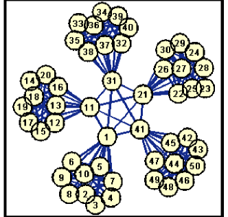
Figure 1: A sample graph with a spectral gap, $\mathcal{G}^{(50,5)}$, created using the procedure described in the text. (The image was created using the graphlayout package for MATLAB written by Matthew Dunham, University of British Columbia.)

Here, $N$ is the total number of oscillators in the system, $\theta_{i}$ and $\omega_{i}$ are the phases and the intrinsic angular frequencies of the individual oscillators, and $K$ is the coupling strength, measuring the influence of every oscillator on the oscillators connected to it. The matrix $A$, the adjacency matrix defining the network structure connecting the oscillators, is defined as follows: $A_{ij}=1$ if oscillators $i$ and $j$ communicate with each other and $A_{ij}=0$ otherwise.

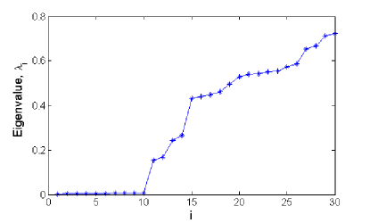
Figure 2: The first 100 eigenvalues of the graph Laplacian corresponding to $\mathcal{G}^{(500,10)}$.

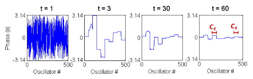
Figure 3: The temporal evolution of the phases of the oscillators at a coupling strength of $K=0.5$. The oscillators in a couple of representative communities (the fourth, $C_{4}$, and ninth, $C_{9}$) are marked in the last plot of the sequence.

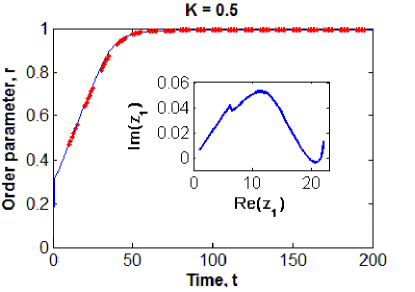
Figure 4: The evolution of the Kuramoto order parameter over time at a coupling strength of $K=0.5$. The results from direct simulation are the solid lines (blue) while the results from coarse projective integration ($5$ time steps for simulation and $5$ for projection) are the dots (red). (The thickness of the plotted dots make the projection step appear shorter). The phase portrait in terms of the real and imaginary components of the first coarse variable (see Eq. 9) is shown in the inset.

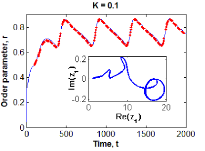
Figure 5: The evolution of the Kuramoto order parameter over time at a coupling strength of $K=0.1$. The results from direct simulation are the solid lines (blue) while the results from coarse projective integration ($25$ time steps for simulation and $25$ for projection) are the dots (red). (The thickness of the plotted dots make the projection step appear shorter). The phase portrait in terms of the real and imaginary components of the first coarse variable (see Eq. 9) is shown in the inset.

For our simulations, we use $500$ oscillators with their intrinsic frequencies sampled from a Gaussian distribution with mean $0$ and standard deviation $1/15$; we will discuss the possibility of different distributions in Section VII. For the underlying connectivity we built a network with a spectral gap, which was observed to lead to low-dimensionality in the long-term system dynamics; this provides the motivation for coarse-graining. The target graph for our illustration was created from a collection of $m$ subgraphs (communities) each containing $s$ nodes; the total number of nodes (oscillators) in the final network was $N=m\times s$. Each subgraph was created using the Watts-Strogatz model Watts and Strogatz (1998), which contains 2 parameters, $k$ - the average degree of the nodes and $p$ - the probability of rewiring. The values of $k$ for the $m$ subgraphs were assigned by uniformly sampling an even number in the interval [14,38] (corresponding to an average degree of approximately 25-75% of the total number of nodes in the sub-graph). The values of $p$ for the individual subgraphs were sampled uniformly in a log scale between 0.001 and 1 (i.e., the values of $log_{10}~{}p$ are sampled uniformly between -3 and 0). The Watts-Strogatz model was chosen to create the constituent subgraphs because it creates graphs ranging from Poisson degree distribution (random) to power law distribution (scale-free) depending on the parameter $p$. Once all the sub-graphs (or communities) are created, a node is randomly chosen from each of the communities to be its leader. Now, all the $m$ leaders are connected to each other resulting in a complete network of leaders (with ${{m}\choose{2}}$ edges). We thus arrive at a connected graph, $\mathcal{G}^{(N,m)}$ with $m$ communities and $N$ nodes in total; a sample resulting graph is shown in Fig. 1 for the case of $m=5$ and $s=10$. In our simulations, we use a graph $\mathcal{G}^{(500,10)}$ created using the same procedure with $m=10$ and $s=50$. The normalized Laplacian of the graph, denoted by $L$, is defined as:

$$L_{ij}:=\left\{\begin{array}[]{cl}1&\text{if }i=j\text{ and }d_{i}\neq 0,\\ -1/\sqrt{d_{i}d_{j}}&\text{if }i\neq j\text{ and }A_{ij}=1,\\ 0&\text{otherwise}\end{array}\right.$$ (2)

where $d_{i}$ is the degree of node $i$.

The normalized Laplacian (in this paper, the term Laplacian should always be taken to mean the normalized graph Laplacian) corresponding to our graph $\mathcal{G}^{(500,10)}$ was computed and its first few eigenvalues (arranged in the ascending order) are plotted in Fig. 2; there is a clear gap in the spectrum after the 10th eigenvalue.

We perform direct simulations of the phase oscillator model (Eq. 1) at different values of coupling strength, with the network topology and oscillator frequencies chosen as described above; the initial phases of the oscillators are sampled from a uniform distribution between $-\pi$ and $\pi$. All our results are reported after the instantaneous average system phase $\arg(\sum_{j}e^{i\theta_{j}})$ has been subtracted (i.e., in a frame that rotates along with the average system phase). At sufficiently large values of coupling strength $K$ we observe (as expected) that the oscillators spontaneously synchronize their frequencies, and their phases “lock” at steady state. Representative phase evolution at such a high coupling strength $K=0.5$ is shown at successive time steps in Fig. 3; note how the community structure of the oscillators quickly becomes visually apparent in the figure.

A quantitative measure of phase synchronization (or coherence in an oscillator population), the so-called order parameter has been defined as:

$$r=\left\|\frac{1}{N}\sum_{j=1}^{N}e^{i\theta_{j}}\right\|.$$ (3)

Its values can range between $0$ and $1$. The higher the value of the order parameter, the higher the degree of synchronization - a value of $1$ indicates the state where all oscillators have the exact same phase. The evolution of this order parameter is shown at a coupling strength of $K=0.5$ as solid lines in Fig. 4. As expected (and confirmed computationally) the steady state value of the order parameter decreases with coupling strength until a critical value of $K_{c}$; below this critical value the oscillators do not synchronize any more, and limit cycle oscillations are observed initially (in parameter space), resulting from a supercritical Hopf bifurcation at $K_{c}$. The evolution of the order parameter at $K=0.1$ depicted by the solid lines in Fig. 5 exhibits such steady limit cycle oscillations.

III Coarse-graining

Our objective is to develop and implement a computer-assisted coarse-grained model of our illustrative coupled oscillator system. The most important step in coarse-graining probably consists of the selection of appropriate coarse observables: a reduced set of variables in terms of which a useful closed description can be obtained. Given suitable coarse variables, it is sometimes possible to derive the reduced equations analytically (in closed form). If, however, the closures required to “write down” the reduced equations in closed form are not known, or cannot be easily approximated, the so-called equation-free framework Kevrekidis et al. (2003, 2004) can be used to computationally implement the reduced model, circumventing its explicit derivation. A brief description of the main points of this modeling/computation framework for complex systems can be found in the Appendix.

In order to motivate our selection of coarse variables, we first identify collective features in the detailed simulation results. Consider the temporal evolution of the oscillator phases as shown in Fig. 3 (for $K=0.5$). In our network $\mathcal{G}^{(N,m)}$, the first $s(=N/m)$ oscillators belong to the first community, the next $s$ to the second community and so on; we define $C_{k}$ as the set containing the indices of all the oscillators in the $k^{th}$ community:

$$C_{k\in[1,m]}=\{(k-1)s+1,(k-1)s+2,...ks\}.$$ (4)

Two oscillators within the same community are connected “more tightly” (they share more common neighbors) than oscillators in different communities. We observe in the simulations that the phases of all the oscillators within a community synchronize with each other at much shorter time scales than those over which the entire network synchronizes. This suggests that, because of the construction of our network topology, its structure can help rationalize the selection of coarse variables appropriate for the long-term dynamics, after initial transients quickly die out. That this separation of time scales leads to low-dimensionality in the system state can be seen in Fig. 3: the randomly initialized individual oscillator phases (our “microscopic” or “fine scale” variables, $U$ in equation-free notation) quickly evolve to “respect” the coarse community structure of the network.

As a result, the following possibilities for coarse variables suggest themselves:

Option 1: Average phase in each community

An obvious choice for a set of coarse variables, $u^{(1)},$ for our example is to use a single common (time-varying) phase angle for each community. The restriction operation (fine states to coarse states in equation-free language) is then defined by assigning the average phase, $\overline{\theta}_{k}$, of all the oscillators in the $k^{th}$ community as the single common phase of that community. The lifting operation (coarse states to consistent fine ones) is implemented by assigning this common phase as the phase angle of all the oscillators in that community.

$$\overline{\theta}_{k}=\frac{1}{s}\sum_{j\in C_{k}}\theta_{j},$$ (5)

$$u^{(1)}=\{\overline{\theta}_{k\in[1,m]}\}.$$ (6)

This apparently intuitive coarse variable selection suffers from two drawbacks. Firstly, partitioning the oscillators into different communities (“clustering” Newman (2006); Nadler et al. (2006); Gfeller and Rios (2008)) is nontrivial for a general network structure (even though -due to the particular construction- it was easy for our example). Even when community structures can be identified, however, this set of coarse variables does not take into account the differences between the different communities and the structure within the communities. This suggests an alternative set of coarse variables that uses the graph Laplacian of the network.

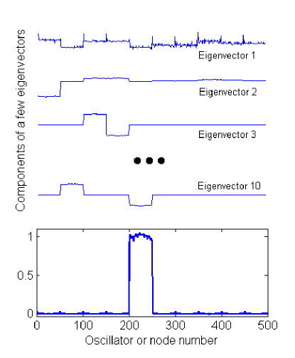
Figure 6: The components of a few eigenvectors of the Laplacian of the graph $\mathcal{G}^{(500,10)}$ are plotted in arbitrary units. The plot (blue line) at the bottom corresponds to a vector that is a linear combination of the first 10 eigenvectors; it is clearly localized to oscillators in the fifth community only. The ten linear combination coefficients are [2.066, 0.259, 0.004, 0.273, -0.323, 0.222, -1.151, 0.017, 4.385, -4.982].

Option 2: Projection to a (truncated) Laplacian eigenbasis

Consider the normalized Laplacian matrix, defined in Eq. 2, for the graph $\mathcal{G}^{(500,10)}$. Let $\lambda_{j}$ be the $j^{th}$ eigenvalue and $\textbf{v}_{j}$ the corresponding normalized eigenvector of the graph Laplacian. From Fig. 2, it can be seen that the first 10 eigenvalues are well separated from the rest (in other words, a spectral gap exists). The components of the eigenvectors of the graph Laplacian corresponding to the ten smallest eigenvalues are plotted as connected dotted lines in Fig. 6. These eigenvectors embody, in an alternative way, the coarse community structure of the entire network. Linear combinations of these eigenvectors can be used to approximately represent any one of the individual communities (as an example, a linear combination of the first 10 eigenvectors whose support lies (approximately) only on the oscillators in the fifth community is shown as a thick solid line in Fig. 6). When only a few eigenvectors capture the presence and structure of the different communities, they form a suitable basis to represent the long term dynamics of the system. A comparison of Figs. 3 and  6 also suggests that a linear combination of these eigenvectors is likely to represent well the long term evolving states of the phase oscillators. In other words, after a short initial transient, the system becomes attracted to a low-dimensional manifold on which the individual oscillator phases can be represented using a lower dimensional basis formed by the first few (here 10) Laplacian eigenvectors of the network; these eigevectors parametrize the low-dimensional manifold.

The use of the graph Laplacian in constructing (coarse) observables is, of course, not new Arenas et al. (2006a, b); McGraw and Menzinger (2007, 2008). Below we will use these variables not only as observables, but as the means to implement accelerated coarse-grained computations with the model. There is a clear analogy between such observables and the use of the finite Fourier transform in solving initial-boundary value problems: instead of eigenfunctions of diffusion in physical space we have eigenvectors of the Laplacian on a graph; instead of evolution equations for time-dependent Fourier mode amplitudes we envision evolution equations for time-dependent components of the system phases on the first few graph Laplacian eigenvectors. Finally, it is also worth pointing out that these eigenvectors are also the eigenvectors of the linearization of the model around the uniform solution of a “nearby” problem: that of coupled identical oscillators Arenas et al. (2006a, b).

We start by defining an $N\times 1$ vector of complex phase angles of the oscillators, $\Theta$:

$$\Theta_{j}=e^{i\theta_{j}};~{}j\in[1,N].$$ (7)

The phase angles should be defined modulo $2\pi$; this complex phase vector correctly represents the phase variable on a unit circle (described by $sin~{}\theta$ and $cos~{}\theta$). We now choose as coarse variables ($u^{(2)}$) the components, $z_{j}$, of this phase vector, $\Theta$, along the direction of the first ten eigenvectors of the graph Laplacian.

$$L\textbf{v}_{j}=\lambda_{j}\textbf{v}_{j};~{}j\in[1,N],$$ (8)

$$u^{(2)}=\{z_{j\in[1,m]}=\textbf{v}_{j}^{T}\mbox{\boldmath$\Theta$}\}.$$ (9)

This projection is our restriction, while translation between the fine description (phases of all the $N$ oscillators) and the coarse description is governed by Eq. 10, our lifting operator.

$$\sum_{j=1}^{m}z_{j}\textbf{v}_{j}\rightarrow\mbox{\boldmath$\Theta$}.$$ (10)

A third option for coarse graining, which includes additional heterogeneity considerations is discussed in Sec. V.

IV Computational Results

IV.1 Coarse projective integration

Using the set of coarse variables $u^{(2)}$, we accelerated the network simulation using coarse projective integration as detailed in the Appendix. Representative results are shown in Figs. 4 and 5, reported in the form of time-series of the order parameter for two values of the coupling strength, above and below $K_{c}$ respectively. For both these cases, the magnitude of the projective step is equal to the duration of the full simulation used to estimate the coarse time derivatives; that is, the full system, Eq. 1, is simulated for only $50\%$ of the overall evolution time. The coarse evolution in both cases clearly follows (in the “eye norm”) the resolved full direct simulation results; this demonstrates the accuracy of the equation-free approach and indirectly validates our selection of coarse variables.

IV.2 Coarse fixed point computation

We performed coarse-fixed point calculations (as outlined in the Appendix) using both choices of coarse variables and compared it to steady states calculated with the full model. Given an initial guess of the $10$ coarse variable steady values, the coarse time-stepper was constructed by lifting, followed by full model simulation (a representative time-stepper horizon was $\tau=10$) and restriction. Fixed points of the coarse time-stepper were arrived at through a Newton-Krylov GMRES iteration Saad and Schultz (1986); Kelley (1995). To quantify accuracy, we calculated the pairwise linear correlation coefficient between the detailed (“fine scale”) phases of the actual fixed point, and those lifted from the converged coarse fixed point values for each choice of coarse variables. The results are reported in Table 1 for three different coupling strengths. The first(respectively, second) row corresponds to results obtained using $u^{(1)}$(respectively, $u^{(2)}$) as coarse variables. Clearly, $u^{(2)}$ gives a more accurate coarse description of the system fixed points compared to just using the average phases in the communities ($u^{(1)}$).

Table 1: Correlation between the detailed phases of the actual fixed point, and those lifted from the converged coarse fixed point values for each choice of coarse variables.

$\rho$	$K=1$	$K=0.5$	$K=0.2$
Using $u^{(1)}$	0.9974	0.9975	0.9976
Using $u^{(2)}$	0.9983	0.9983	0.9983
Using $u^{(3)}$	0.9994	0.9994	0.9995

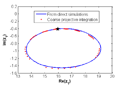
Figure 7: A coarse limit cycle computed from direct simulations at a coupling strength of $K=0.1$ is plotted using a solid (blue) line. The star (black) corresponds to the solution (the point on a Poincaré map) obtained using a coarse limit cycle solver. This point is then used as the initial condition for coarse projective integration (red dots); the coarse trajectory returns to that point after one period.

IV.3 Coarse limit cycle computation

We have already discussed the existence of stable limit cycle oscillations below (and close to) the critical coupling strength, $K_{c}$. The limit cycle found out from direct simulations for $K=0.1$ is plotted as a solid line in the phase space projection on the real and imaginary parts of $z_{1}$ in Fig. 7. We also find a (coarse) point on this limit cycle by locating the (coarse) fixed point of an appropriate (coarse) Poincaré map; the point is represented as a star in Fig. 7. This point (as well as the period of the coarse limit cycle) is found by solving (again through Newton-Krylov GMRES) Eq. 18 for the appropriate set of values of the coarse variables $u^{(2)}$; the Poincaré map was defined in terms of the $Re(z_{1})$ coarse variable. In these computations, the full system was simulated for the entire Poincaré return time; but the map, and the Newton fixed point computation were performed in the reduced space of the coarse variables. In an extra validation step, the trajectory around the limit cycle was followed through coarse projective integration (see Fig. 7), and seen to coincide visually with the (phase space projection of the) full simulation limit cycle.

These representative computations confirm that computational coarse-graining (with the appropriate selection of coarse variables) can be used to effectively perform computations with the (explicitly unavailable) coarse-grained model. Coarse projective integration, coarse fixed point and limit cycle computations (and also, easily, coarse stability and continuation computations) can be implemented in the form of computational “wrappers” around the full simulation. The choice of coarse variables (and the associated lifting and restriction steps) form a critical part of the approach; an improvement on this process is presented below.

V The effect of oscillator heterogeneity

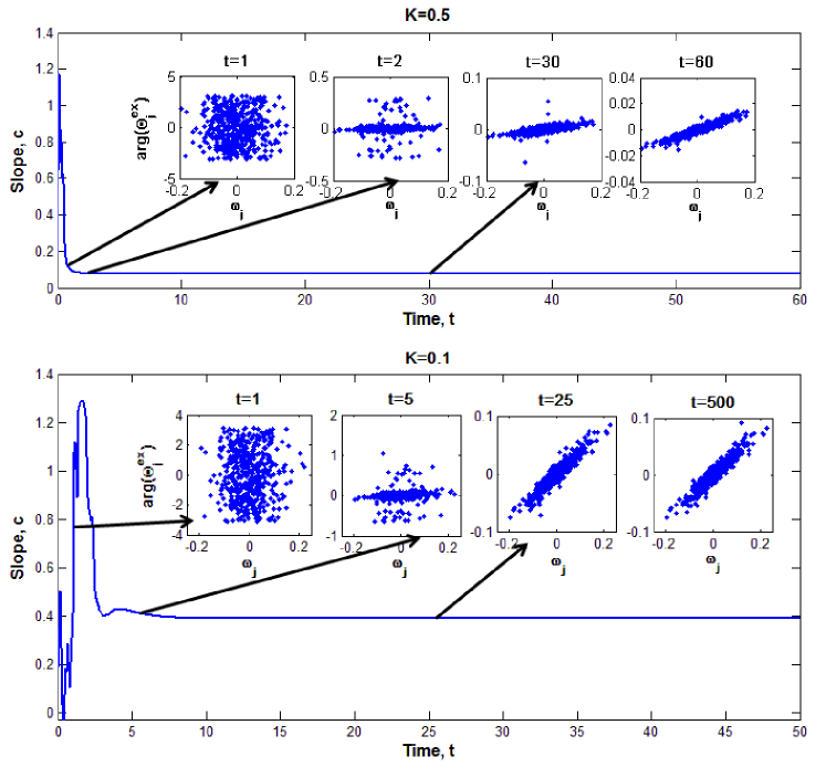
Figure 8: Evolution of the slope $c$ of the linear fit between excess phase and angular frequency for $K=0.5$ and $K=0.1$. Insets: Plots of excess phases $arg(\Theta_{j}^{ex})$ versus oscillator angular frequencies $\omega_{j}$ at a few representative temporal instances.

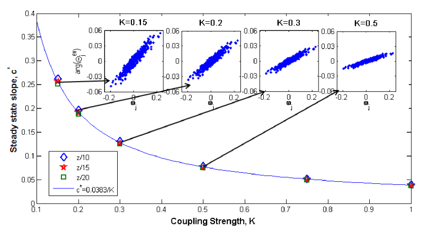
Figure 9: Steady state values of slope $c^{*}$ of the linear correlation between excess phase and intrinsic oscillator angular frequency plotted as a function of the coupling strength $K$. The labels $z/10$, $z/15$ and $z/20$ in the legend denote the three different distributions from which the intrinsic oscillator frequencies are sampled, $z$ representing a standard normal random variable). The inverse proportionality can be seen from the curve fit, $c^{*}=0.0383/K$. Insets: Plots of excess phases $arg(\Theta_{j}^{ex})$ versus oscillator angular frequencies $\omega_{j}$ at steady state for a few values of coupling strength.

In our coarse graining efforts, so far, we have focused on the structure of the network and ignored the effect of the heterogeneity in the angular frequencies of the oscillators. In this section we present a systematic approach to taking this heterogeneity into account in the coarse-graining procedure. The motivation comes from the observation, in the literature Moon et al. (2006), that for all-to-all coupling (that is, in the absence of fine network structure) the oscillator phases will, under certain conditions, become quickly correlated with their intrinsic frequencies. We have observed the same phenomenon in our, more structured, networks: the sequence of insets in Fig. 8 shows the transient evolution of the (“excess”) phase of the oscillators in our network plotted against their individual frequencies. The term “excess phase”, $\mbox{\boldmath$\Theta$}^{ex}$, here refers to the portion of the phase vector that is not captured by the projection on the first 10 Laplacian eigenvectors; using Eq. 11 we plot the complex argument of each oscillator, viz., $arg(\Theta_{j}^{ex})$ against $\omega_{j}$.

$$\mbox{\boldmath$\Theta$}^{ex}=\mbox{\boldmath$\Theta$}-\sum_{j=1}^{m}\textbf{v}_{j}^{T}\mbox{\boldmath$\Theta$}\textbf{v}_{j},$$ (11)

What we see is that, even when the oscillators are initialized with random phases (in the form of the “cloud” seen in the first inset), they very quickly (visibly by time $t=2$ and almost quantitatively by $t=30$) develop a strong, stationary correlation with the intrinsic frequencies. These plots confirm the existence of a strong linear correlation between the “excess phase” and the angular frequencies of the oscillators. The evolution of the slope of the best linear fit is plotted in Fig. 8 (a) and (b) for different values of the coupling strength $K$.

A number of additional observations can be made from these plots. The time taken for the correlation slope $c$ to approach steady state is much less than the time scale in which the order parameters reach steady state (compare with Figs. 4 and 5). Even for the case of $K=0.1$, corresponding to stable limit cycle oscillations, the values of $c$ do not vary much once the stable limit cycle is approached. Fig. 9 shows how this (quickly achieved) steady state correlation slope varies with the oscillator coupling strength. For a range of coupling strengths, this steady state value of $c$ is obtained for three different frequency distributions (the oscillator frequencies were sampled from the normal distribution with mean $0$ and standard deviation of $1/10$, $1/15$ and $1/20$ respectively.) The steady state correlation between excess phase and frequency appears to be independent of the range of (or the variance in) the oscillator frequencies. Fig. 9 and its insets quantify the dependence of the correlation on $K$; the steady state values of $c$ are seen to decrease with coupling strength as one might expect (since, at higher coupling strengths, the oscillator phases should exhibit less variance). In particular, an approximate inverse proportionality is computationally observed between the coupling strength $K$, and the steady slope $c^{*}$, quantified by the following fitted curve:

$$c^{*}=0.0383/K.$$ (12)

We find it remarkable that our “decoupled” procedure, which first considers heterogeneity in the network structure, and only then considers heterogeneity in the oscillator intrinsic properties gives us so robust features for the network dynamics. Note that the constant $0.0383$ applies only for the particular network used in the simulation shown. For different network structure realizations, the constant will be different.

Based on these results, we can now integrate the effects of both network structure and oscillator frequency distribution in the coarse-graining of the oscillator phases (in particular, in our lifting operator).

VI Coarse-graining the heterogeneous oscillators

The discussions in Section. V suggest that capturing the correlation between excess phase and intrinsic oscillator frequency can lead to a better set of coarse variables and a more accurate lifting operator for the coarse-graining process. For our illustrative example, a single additional variable, the slope $c$ is, as we will show, sufficient in capturing this correlation. Before we demonstrate this, however, we note the more general question: for arbitrary heterogeneity distributions (not just Gaussian as the one studied here), what is the nature and number of additional coarse variables necessary to quantitatively account for the frequency heterogeneity? We will return to this question in the last Section.

Using the single scalar slope $c$ as an additional coarse variable, we define the “corrected” vector of complex phase angles, $\widetilde{\Theta}$, similar to $\Theta$, but now taking the $c\omega_{j}$ into account:

$$\mbox{$\widetilde{\Theta}_{j}$}=e^{i(\theta_{j}-c\omega_{j})};~{}j\in[1,N],$$ (13)

$$\sum_{j=1}^{m}z_{j}\textbf{v}_{j}\rightarrow\mbox{\boldmath$\widetilde{\Theta}$}.$$ (14)

Our corrected lifting operation, going beyond the first $m$ (here, 10) eigenvectors of the graph Laplacian, is given by Eqs. 13 and  14. For the corrected restriction operation, the vector of phase angles is initially projected on the first $10$ graph Laplacian eigenvectors to obtain the $z_{j}$; the “excess phases” are then used to estimate the slope $c$ through linear regression. Our augmented set of coarse variables now reads:

$$u^{(3)}=\{z_{j\in[1,m]}=\textbf{v}_{j}^{T}\mbox{\boldmath$\widetilde{\Theta}$},c\}.$$ (15)

The results of computational coarse graining with the coarse variable set $u^{(3)}$ are, as one might expect, qualitatively similar to, but more accurate than, the results with the coarse set $u^{(2)}$ presented in Sec. IV.

Note that since (as we computationally observed) $c$ quickly approaches an approximately constant value $c^{*}$ for each specific system realization, we can -in studying long term dynamics- fix its value at $c^{*}$ and not even consider it as an extra dynamic coarse variable. The constant value $c^{*}$ for different coupling strengths can also be inferred from formulas like Eq. 12.

Each successive coarse variable choice $u^{(1)}$, $u^{(2)}$ and $u^{(3)}$ clearly includes more information about the system than the previous one: the coarse variable set $u^{(1)}$ just accounts for the presence of different communities, $u^{(2)}$ accommodates the structure of the different communities while set $u^{(3)}$ considers the influence of the heterogeneous frequencies of the oscillators as well. In order to quantify whether this additional information is also meaningful, we compared the results of coarse fixed point analysis using the three choices of coarse variables. The results in Table 1 demonstrate that the additional information included in successive choices of coarse variable sets actually leads to more accurate computation of the system features (in particular, its coarse steady states).

VII Conclusions

We have demonstrated an approach to coarse-graining the computations of the (long-term) dynamics of networks of coupled heterogeneous oscillators; our approach was based on the equation-free framework, and was able to account -in separate steps- for the network structure and the oscillator intrinsic heterogeneity. The effect of the network structure on the evolution of the individual oscillator phases was first accounted for using the spectral properties of the network (under the assumption that the network graph Laplacian possesses a spectral gap). In a second step, the effect of the heterogeneity in oscillator frequencies was accounted for by observing (and then capturing) a strong correlation between (“excess”) phase angles and intrinsic oscillator frequency distribution. Both steps were incorporated in the construction of a lifting and a restriction operator (from coarse variables to detailed, fine scale state consistent realizations and vice versa). These operators can then be linked, in the equation-free framework, with algorithms such as coarse fixed point and coarse limit cycle computations, as well as with coarse projective integration, all of which were demonstrated.

Even though the individual oscillator dynamics and the network topology used for illustration here were relatively simple, we are confident that the procedures demonstrated here can be extended to different, more complex individual oscillator dynamics and for other types of networks, as long as they possess spectral gaps as well. Extensions to networks of spiking neurons, which can also be considered as coupled oscillators -but with much more complex, and especially directional coupling topologies- is probably too ambitious with only these tools. As pointed out in Ref. Binzegger et al. (2009), “The information required to construct a detailed and specific configuration of neocortex containing some $\mathit{10^{12}}$ connections exceeds by far the roughly $\mathit{10^{8}}$ bits of information available in the genome for specification of the entire organism. On these grounds alone it appears that nature’s strategy for construction of the neocortex must depend on the dynamic assembly of rather specific but simple modules”. This reasoning supporting “module simplicity and specificity” provides hope and motivation for the deployment of reductionist approaches in such systems Laing and Lord (2009).

One particular direction of extension for which we are more confident, and which we are currently pursuing, is the study of diverse heterogeneity distributions. In our illustrative example, the (intrinsic frequency) heterogeneity distribution was simply a normal one (with different variances). A single scalar quantity (the slope, $c$) of the correlation between heterogeneity and system state was sufficient to improve our coarse description here. This slope is but the first nontrivial coefficient of an expansion of the system state (here, the excess phases) as a function of a random variable (here, the intrinsic frequency). In effect, this is a “one-term” polynomial chaos Ghanem and Spanos (1991) expansion of a function of a random variable (the oscillator frequency) with a particular probability distribution. It is straightforward to use different expansions (depending on the distribution of the random variable, different hierarchies of polynomials are applicable, see for example the Askey scheme Xiu and Karniadakis (2002)); it is also straightforward to use more than one term in the expansion in a particular polynomial set if the correlation exhibits more structure than the straight line we observed here. This research avenue provides a direct link between existing and developing tools in the study of uncertainty quantification (polynomial chaos approaches, and the associated collocation schemes) with the study of coupled heterogeneous oscillator problems, even when heterogeneity arises in more than one properties of the coupled system. One particularly interesting direction for network dynamics arises when the oscillator behavior depends crucially on the degree of this oscillator in the overall network. If correlations between node degrees and oscillator states quickly develop in system startup transients, the tools we outlined above may well serve in successful coarse-graining of the overall network dynamics.

*

Appendix A Outline of the Equation-Free Framework

The Equation-Free (EF) approach to modeling and computation for complex/multiscale systems has been developed for problems that can, in principle, be described at multiple levels. In particular, it is applicable to systems for which the evolution equations are available at a “fine” (atomistic, microscopic, individual-based) scale, while the equations for the “coarse” (macroscopic, system level) behavior, which is of interest, are not available in closed form. We will illustrate the EF approach through a brief description of coarse projective integration and coarse fixed point computation. The system of interest is completely specified at any moment in time by a set of fine or microscopic variables $U$. We start with the assumption that an appropriate set of coarse variables $u$ (observables in terms of which closed equations can in principle be written at the macroscopic level) have been selected. We also assume that good lifting ($\mathcal{L}[\cdot$]) and restriction ($\mathcal{R}[\cdot]$) operators are available: the lifting creates fine scale initial conditions consistent with prescribed values of macroscopic observables, while the restriction obtains the values of the observables from a fine scale state. These operators effectively “translate” fine scale states to the corresponding coarse ones, and coarse ones to consistent fine ones respectively.

For our illustrative example, the “fine scale” state at a time instance $t_{i}=i\Delta t$ is the vector of phase angles of all oscillators $U(t_{i})$, while the corresponding set of coarse variable values is $u(t_{i})$. A coarse projective integration step consists of the following sub-steps:

1. Lifting step: Start with initial condition $u(0)$ for the coarse macroscopic variables and lift them to a consistent microscopic description: $U(0)=\mathcal{L}[u(0)]$.

2. Evolve the oscillators using $U(0)$ as the initial condition for their phases in the microscopic simulator for a time $t_{h}$, long enough for the fast components of the dynamics to equilibrate, but short compared to the slow (coarse) system time scales (see Kevrekidis et al. (2003)). The final state of this step is $U(t_{h})$.

3. Evolve the microscopic variables, $U(0)$, for additional $k$ time steps, generating the values $U(t_{i})$, $i=h+1$ to $h+k$, i.e., $U(t_{h+k})=\mathcal{E}_{t_{h+k}}[U(0)]$.

4. Restriction step: Obtain the restrictions, $u(t_{i})=\mathcal{R}[U(t_{i})]$, $i=h+1$ to $h+k$.

5. Projective step: Estimate time derivatives from these restrictions, $u(t_{i})$, $i=h+1$ to $h+k$, and use any numerical scheme (the simplest one would be forward Euler) to “project” the macroscopic variables “into the future” over a time interval $p\Delta t$ to obtain $u(t_{h+k+p})$.

One then uses these projected values of the coarse variables as the initial condition in repeating the overall procedure.

Using the lifting and restriction operations, and the fine-scale system simulator, one can define a coarse time-stepper $\Phi_{\tau}$ (Eq. 16) that takes as input the coarse variables at a given time, $u(t)$, and outputs the coarse variables at a later time, $u(t+\tau)$.

$$u(t+\tau)=\Phi_{\tau}[u(t)]=\mathcal{R}[\mathcal{E}_{\tau}[\mathcal{L}[u(t)]]].$$ (16)

One can also use such a coarse time-stepper to find the coarse fixed points, $\widehat{u}$, by solving Eq. 17 for (in principle) any time $\tau$, using matrix-free implementations of algorithms like Newton-Krylov-GMRES Saad and Schultz (1986); Kelley (1995) to iteratively solve sets of nonlinear equations.

$$\widehat{u}=\Phi_{\tau}[\widehat{u}].$$ (17)

With the help of coarse Poincaré maps, one can solve a similar equation to find a (coarse) point on the (coarse) limit cycle, $\widetilde{u}$, as well as its period, $T$.

$$\widetilde{u}=\Phi_{T}[\widetilde{u}].$$ (18)

Matrix-free implementations of eigensolvers (e.g. matrix-free Arnoldi procedures Lehoucq et al. (1998)) can (and have been) used to characterize the coarse linearized stability of coarse fixed points and limit cycles Samaey et al. (2008); Siettos et al. (2003); Lust and Roose (1998).