Opportunities for Network Coding:
To Wait or Not to Wait

Abstract

It has been well established that wireless network coding can significantly improve the efficiency of multi-hop wireless networks. However, in a stochastic environment some of the packets might not have coding pairs, which limits the number of available coding opportunities. In this context, an important decision is whether to delay packet transmission in hope that a coding pair will be available in the future or transmit a packet without coding. The paper addresses this problem by formulating a stochastic dynamic program whose objective is to minimize the long-run average cost per unit time incurred due to transmissions and delays. In particular, we identify optimal control actions that would balance between costs of transmission against the costs incurred due to the delays. Moreover, we seek to address a crucial question: what should be observed as the state of the system? We analytically show that observing queue lengths suffices if the system can be modeled as a Markov decision process. We also show that a stationary threshold type policy based on queue lengths is optimal. We further substantiate our results with simulation experiments for more generalized settings.

An earlier version of this paper was presented at the ISIT, 20111.

I Introduction

In recent years, there has been a growing interest in the applications of network coding techniques in wireless networks. It was shown that network coding can result in significant improvements in the performance in terms of delay and transmission count. For example, consider a wireless network coding scheme depicted in Fig. 1(a). Here, wireless nodes 1 and 2 need to exchange packets $x_{1}$ and $x_{2}$ through a relay node (node 3). A simple store-and-forward approach needs four transmissions. In contrast, the network coding solution uses a store-code-and-forward approach in which the two packets $x_{1}$ and $x_{2}$ are combined by means of a bitwise XOR operation at the relay and are broadcast to nodes 1 and 2 simultaneously. Nodes 1 and 2 can then decode this coded packet to obtain the packets they need.

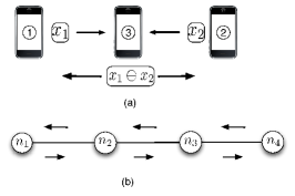
Figure 1: (a) Wireless Network Coding (b) Reverse carpooling.

Effros et al. [1] introduced the strategy of reverse carpooling that allows two information flows traveling in opposite directions to share a path. Fig. 1(b) shows an example of two connections, from $n_{1}$ to $n_{4}$ and from $n_{4}$ to $n_{1}$ that share a common path $(n_{1},n_{2},n_{3},n_{4})$. The wireless network coding approach results in a significant (up to 50%) reduction in the number of transmissions for two connections that use reverse carpooling. In particular, once the first connection is established, the second connection (of the same rate) can be established in the opposite direction with little additional cost.

In this paper, we focus on the design and analysis of scheduling protocols that exploit the fundamental trade-off between the number of transmissions and delay in the reverse carpooling schemes. In particular, to cater to delay-sensitive applications, the network must be aware that savings achieved by coding may be offset by delays incurred in waiting for such opportunities. Accordingly, we design delay-aware controllers that use local information to decide whether or not to wait for a coding opportunity, or to go ahead with an uncoded transmission. By sending uncoded packets we do not take advantage of network coding, resulting in a penalty in terms of transmission count, and, as a result, energy-inefficiency. However, by waiting for a coding opportunity, we might be able to achieve energy efficiency at the cost of a small delay increase.

Consider a relay node that transmits packets between two of its adjacent nodes with flows in opposite directions, as depicted in Fig. 2. The relay maintains two queues $q_{1}$ and $q_{2}$, such that $q_{1}$ and $q_{2}$ store packets that need to be delivered to node 2 and node 1, respectively. If both queues are not empty, then it can relay two packets from both queues by performing an XOR operation. However, what should the relay do if one of the queues has packets to transmit, while the other queue is empty? Should the relay wait for a coding opportunity or just transmit a packet from a non-empty queue without coding? This is the fundamental question we seek to answer. In essence we would like to trade off efficiently transmitting the packets against high quality of service (i.e., low delays).

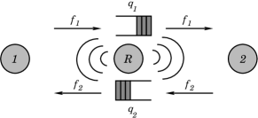
Figure 2: 3-Node Relay Network.

I-A Related Work

Network coding research was initiated by the seminal work of Ahlswede et al. [2] and since then attracted major interest from the research community. Network coding technique for wireless networks has been considered by Katti et al. [3]. They propose an architecture, referred to as COPE, which contains a special network coding layer between the IP and MAC layers. In [4], an opportunistic routing protocol is proposed, referred to as MORE, that randomly mixes packets that belong to the same flow before forwarding them to the next hop. In addition, several works, e.g., [5, 6, 7, 8, 9, 10], investigate the scheduling and/or routing problems in the network coding enabled networks. Sagduyu and Ephremides [5] focus on the network coding in the tandem networks and formulate related cross-layer optimization problems, while Khreishah et al. [6] devise a joint coding-scheduling-rate controller when the pairwise intersession network coding is allowed. Reddy et al. [7] have showed how to design coding-aware routing controllers that would maximize coding opportunities in multihop networks. References [8] and [9] attempt to schedule the network coding between multiple-session flows. Xi and Yeh [10] propose a distributed algorithm that minimizes the transmission cost of a multicast session.

The work of Ciftcioglu et al. [11] is the most relevant to our paper. It is important to note that this work was performed independently and analyzed a related problem from a different perspective. In particular, [11] proposed a control policy that strikes a balance between the delay and the cost, as well as compares the policy to one that never waits for the coding opportunity. In contrast, in our paper, we provide a provably optimal control policy and identify its structure.

In this paper, we consider a stochastic arrival process and address the decision problem of whether or not a packet should wait for a coding opportunity. Our objective is therefore to study the delicate trade-off between the energy consumption and the queueing delay when network coding is an option. We use the Markov decision process (MDP) framework to model this problem and formulate a stochastic dynamic program that determines the optimal control actions in various states. While there exists a large body of literature on the analysis of MDPs (see, e.g., [12, 13, 14, 15]), there is no clear methodology to find optimal policies for the problems that possess the proprieties of infinite horizon, average cost optimization, and with a countably infinite state space. Indeed, [15] remarks that it is difficult to analyze and obtain optimal policies for such problems. The works in [16, 17, 18, 19] contribute to the analysis of MDPs with countably infinite state space. Moreover, reference [20] that surveys the recent results on the monotonic structure of optimal policy, states that while one dimensional MDP with convex cost functions has been extensively studied, limited models for multi-dimensional spaces are dealt with due to the correlations between dimensions. In many high-dimension cases, one usually directly investigates the properties of the cost function. As we will see later, this paper poses precisely such a problem, and showing the properties of optimal solution is one of our main contributions.

I-B Main Results

We first consider the case illustrated in Fig. 2, in which we have a single relay node with two queues that contain packets traversing in opposite directions. We assume that time is slotted, and the relay can transmit at most one packet during each time slot. We also assume that the arrivals into each queue are independent and identically distributed. Each transmission by the relay incurs a cost, and similarly, each time slot when a packet waits in the queue has some cost. We would like to minimize the average sum of the two costs. In general, we could utilize a controller that belongs to one of the following sets [12]:

• $\Pi^{\text{HR}}$ - a set of randomized history dependent policies;

• $\Pi^{\text{MR}}$ - a set of randomized Markov policies;

• $\Pi^{\text{SR}}$ - a set of randomized stationary policies;

• $\Pi^{\text{SD}}$ - a set of deterministic stationary policies.

It is not hard to see (as shown in [12]) that

$$\Pi^{\text{SD}}\subset\Pi^{\text{SR}}\subset\Pi^{\text{MR}}\subset\Pi^{\text{HR}}.$$

The complexity of the algorithms increases from left to right above: in what regime does the solution to our problem lie? We can think of the system state as the two queue lengths. We find that the optimal policy is a simple queue-length threshold policy with one threshold for each queue at the relay, and whose action is simply: if a coding opportunity exists, code and transmit; else transmit a packet if the threshold for that queue is reached. We then show how to find the optimal thresholds. Thus, our result implies that although waiting time information might be available, we do not need to actually use it.

We examine two general models afterward. In the first model, the service capacity of the relay is not restricted to one packet per time slot. Then, if the relay can serve a batch of packets, we find that the optimal controller is of the threshold type for one queue, when the queue length of the other queue is fixed. Secondly, we study an arrival process with memory (Markov modulated). Here, we discover that the optimal policy has multiple thresholds.

We then perform a numerically study of a number of policies that are based on waiting time and queue length, waiting time only, as well as the optimal deterministic queue-length threshold policy to indicate the potential of our approach. We also evaluate the performance of a deterministic queue length based policy in the line network topology via simulations.

Contributions. Our contributions can be summarized as follows. We introduce the problem of delay versus coding efficiency trade-off, as well as formulate it as an MDP problem and obtain the structure of the optimal policy. It turns out that the optimal policy does not use the waiting time information. Moreover, we prove that the optimal policy is stationary and of threshold type in terms of the queue lengths, and therefore is easy to implement. While it is easy to analyze MDPs that have a finite number of states, or involve a discounted total cost optimization with a single communicating class, our problem does not possess any of these properties. Hence, although our policy is simple, the proof is extremely intricate. Furthermore, our policy and proof techniques can be extended to other scenarios such as batched service and Markov-modulated arrival process.

II System Overview

II-A System model

Consider a multi-hop wireless network operating a time-division multiplexing scheme to store and forward packets from various sources to destinations. Time is divided into slots that are further divided into mini-slots. In each slot, each node is allowed to transmit in its assigned mini-slot. Such a deterministic schedule without interference is easy to construct, e.g., see [21, 22] for a method to do so in a unit square with randomly dropped nodes, in which every node gets a transmission opportunity with finite periodicity.

Our first focus is on the case of a single relay node of interest, which has the potential for network coding packets from flows in opposing directions. Consider Fig. 2 again. We call the two adjacent nodes to the relay $R$ as nodes $1$ and $2$. We assume that there is a flow $f_{1}$ that goes from node $1$ to $2$ and another flow $f_{2}$ from node $2$ to $1$, both of which are through the relay under consideration. The packets from both flows are stored at separate queues, $q_{1}$ and $q_{2}$, at node $R$. Each slot is divided into several mini-slots, such that the last mini-slot is used by the relay and all other mini-slots are used by nodes $1$ and $2$. Note that the time period between transmission opportunities for the relay is precisely one slot.

The number of arrivals between consecutive slots to both flows is assumed to be independent of each other and also independent and identically distributed (i.i.d.) over time, with the random variables $\mathcal{A}_{i}$ for $i=1,2$ respectively. In each slot, $n$ packets arrive at $q_{i}$ with the probability $\mathbb{P}(\mathcal{A}_{i}=n)=p^{(i)}_{n}$ for $n\in\mathbb{N}\cup\{0\}$. Afterward, the relay gets an opportunity to transmit. Initially we assume that the relay can transmit a maximum of one packet in each time slot.

II-B Markov Decision Process Model

We use a Markov decision process (MDP) model to develop a strategy for the relay to decide its best course of action at every transmission opportunity. For $i=1,2$ and $t=0,1,2,\cdots$, let $Q^{(i)}_{t}$ be the number of packets in $q_{i}$ at the $t^{\text{th}}$ time slot just before an opportunity to transmit. Let $a_{t}$ be the action chosen at the end of the $t^{\text{th}}$ time slot with $a_{t}=0$ implying the action is to do nothing and $a_{t}=1$ implying the action is to transmit. Clearly, if $Q^{(1)}_{t}+Q^{(2)}_{t}=0$, then $a_{t}=0$ because that is the only feasible action. Also, if $Q^{(1)}_{t}Q^{(2)}_{t}>0$, then $a_{t}=1$ because the best option is to transmit as a coded XOR packet as it reduces both the number of transmissions as well as latency. However, when exactly one of $Q^{(1)}_{t}$ and $Q^{(2)}_{t}$ is non-zero, it is unclear what the best action is.

To develop a strategy for that, we first define the costs for latency and transmission. Let $C_{T}$ be the cost for transmitting a packet and $C_{H}$ be the cost of holding a packet for a length of time equal to one slot. Without loss of generality, we assume that if a packet is transmitted in the same slot that it arrived, its latency is zero. Also, the cost of transmitting a coded packet is the same as that of a non-coded packet. That said, our objective is to derive an optimal policy that minimizes the long-run average cost per slot. Therefore, we define the MDP$\{(Q_{t},a_{t}),t\geq 0\}$ where $Q_{t}=(Q^{(1)}_{t},Q^{(2)}_{t})$ is the state of the system and $a_{t}$ the control action chosen by the relay at the $t^{\text{th}}$ slot. The state space (i.e., all possible values of $Q_{t}$) is the set $\{(i,j):i=0,1,\cdots;j=0,1,\cdots\}$.

Let $C(Q_{t},a_{t})$ be the immediate cost if action $a_{t}$ is taken at time $t$ when the system is in state $Q_{t}=(Q^{(1)}_{t},Q^{(2)}_{t})$. Therefore,

$$C(Q_{t},a_{t})=C_{H}([Q^{(1)}_{t}-a_{t}]^{+}+[Q^{(2)}_{t}-a_{t}]^{+})+C_{T}a_{t},$$ (1)

where $[x]^{+}=\max(x,0)$. The long-run average cost for some policy $\theta\in\Pi^{\text{HR}}$ is given by

$$V(\theta)=\lim_{K\rightarrow\infty}\frac{1}{K+1}\mathbb{E}_{\theta}\left[\sum_{t=0}^{K}C(Q_{t},a_{t})|Q_{0}=(0,0)\right],$$ (2)

where $\mathbb{E}_{\theta}$ is the expectation operator taken for the system under policy $\theta$. Notice that our initial state is an empty system, although the average cost would not depend on it. Our goal is to characterize and obtain the average-optimal policy, i.e., the policy that minimizes $V(\theta)$. We first describe the probability law for our MDP and then in subsequent sections develop a methodology to obtain the average-optimal policy.

For the MDP$\{(Q_{t},a_{t}),t\geq 0\}$, let $P_{a_{t}}(Q_{t},Q_{t+1})$ be the transition probability from state $Q_{t}$ to $Q_{t+1}$ associated with action $a_{t}\in\{0,1\}$. Then the probability law can be derived as $P_{0}\left((i,j),(k,l)\right)=p^{(1)}_{k-i}p^{(2)}_{l-j}$ for all $k\geq i$ and $l\geq j$; otherwise, $P_{0}\left((i,j),(k,l)\right)=0$. Also, $P_{1}\left((i,j),(k,l)\right)=p^{(1)}_{k-[i-1]^{+}}p^{(2)}_{l-[j-1]^{+}}$ for all $k\geq[i-1]^{+}$ and $l\geq[j-1]^{+}$; otherwise, $P_{1}\left((i,j),(k,l)\right)=0$.

A list of important notation used in this paper is summarized in Table I.

$\mathcal{A}_{i}$	Random variable that represents the number of packets that arrives at $q_{i}$ for each time slot
$p^{(i)}_{n}$	Probability that $n$ packets arrive at $q_{i}$, i.e., $\mathbb{P}(\mathcal{A}_{i}=n)$
$Q^{(i)}_{t}$	The number of packets in $q_{i}$ at time $t$
$Q_{t}$	System state, i.e., $(Q^{(1)}_{t},Q^{(2)}_{t})$
$a_{t}$	Action chosen by relay at time $t$
$C_{T}$	Cost of transmitting one packet
$C_{H}$	Cost of holding a packet for one time slot
$C(Q_{t},a_{t})$	Immediate cost if action $a_{t}$ is taken at time $t$ when the system is in state $Q_{t}$
$V(\theta)$	Time average cost under the policy $\theta$
$P_{a_{t}}(Q_{t},Q_{t+1})$	Transition probability from state $Q_{t}$ to $Q_{t+1}$ when action $a_{t}$ is chosen
$V_{\alpha}(i,j,\theta)$	Total expected discounted cost under the policy $\theta$ when the initial state is $(i,j)$
$V_{\alpha}(i,j)$	Minimum total expected discounted cost when the initial state is $(i,j)$, i.e., $\min_{\theta}V_{\alpha}(i,j,\theta)$
$v_{\alpha}(i,j)$	Difference of the minimum total expected discounted cost between the states $(i,j)$ and $(0,0)$, i.e., $V_{\alpha}(i,j)-V_{\alpha}(0,0)$
$V_{\alpha,n}(i,j)$	Iterative definition for the optimality equation of $V_{\alpha}(i,j)$
$\mathcal{V}_{\alpha}(i,j,a)$	$V_{\alpha}(i,j)=\min_{a\in\{0,1\}}\mathcal{V}_{\alpha}(i,j,a)$, which is the optimality equation of $V_{\alpha}(i,j)$
$\Delta\mathcal{V}(i,j)$	$\mathcal{V}_{\alpha}(i,j,1)-\mathcal{V}_{\alpha}(i,j,0)$

TABLE I: Notation table

III Should we maintain waiting time information?

As described in the previous section, our goal is to obtain the average-optimal policy. To that end, we first find the space of possible policies and then identify the average-optimal policy within this space. Our first question is: what is the appropriate state space? Is it just queue length, or should we also consider waiting time?

Intuition tells us that if a packet has not been waiting for a long time then perhaps it could afford to wait a little more, but if a packet has waited for long, it might be better to just transmit it. That seems logical considering that we try our best to code but we cannot wait too long because it hurts in terms of holding costs. It is easy to keep track of waiting time information using time-stamps on packets when they are issued. Let $T^{(i)}$ be the arrival time of $i^{\text{th}}$ packet and $\mathcal{D}^{(i)}_{\theta}$ be its delay (i.e., the waiting time before it is transmitted) while policy $\theta$ is applied. We also denote by $\mathcal{T}_{t,\theta}$ the number of transmissions by time $t$ under policy $\theta$. Then Eq. (2) can be written as

$$V(\theta)=\lim_{K\rightarrow\infty}\frac{1}{K+1}\mathbb{E}_{\theta}\left[\sum_{i:T^{(i)}\leq K}C_{H}\mathcal{D}^{(i)}_{\theta}+C_{T}\mathcal{T}_{K,\theta}\right].$$ (3)

Would we be making better decisions by also keeping track of waiting times of each packet? We answer this question in Proposition 2 that requires the following lemma, which indeed holds for generic MDPs [12].

Lemma 1 ([12], Theorem 5.5.3).

For an MDP$\{(Q_{t},a_{t}),t\geq 0\}$, given any randomized history dependent policy and starting state, there exists a randomized Markov policy with the same long-run average cost.

Proposition 2.

• For the MDP$\{(Q_{t},a_{t}),t\geq 0\}$, if there exists a randomized history dependent policy that is average-optimal then there exists a randomized Markov policy $\theta^{*}\in\Pi^{\text{MR}}$ that minimizes $V(\theta)$.

• Further, one cannot find a policy which also uses waiting time information that would yield a better solution than $V(\theta^{*})$.

Proof.

The first result immediately follows from Lemma 1. Now, we focus on the second result. We notice that knowing the entire history of states (i.e., the number of packets in the queues) and actions one can always determine the history of waiting times as well as the current waiting times of all packets. Therefore the average-optimal policy $\theta^{\prime}$ that uses waiting time information is equivalent to a history dependent policy. From Lemma 1, we can always find a randomized Markov policy that yields the same average-optimal solution as $V(\theta^{\prime})$. ∎

IV Structure of the Average-Optimal Policy - Stationary and Deterministic Property

In the previous section, we showed that there exists an average-optimal policy that does not include the waiting time in the state of the system. Next, we focus on queue length based and randomized Markov policies, as well as determine the structure of the average-optimal policy. In this section, we will show that there exists an average-optimal policy that is stationary and deterministic.

We begin by considering the infinite horizon $\alpha$-discounted cost case, where $0<\alpha<1,$ which we then tie to the average cost case. This method is typically used in the MDP literature (e.g., [19]), where the conditions for the structure of the average-optimal policy usually rely on the results of the infinite horizon $\alpha$-discounted cost case. For our MDP$\{(Q_{t},a_{t}),t\geq 0\}$, the total expected discounted cost incurred by a policy $\theta\in\Pi^{\text{HR}}$ is

$$V_{\alpha}(i,j,\theta)=\mathbb{E}_{\theta}\left[\sum_{t=0}^{\infty}\alpha^{t}C(Q_{t},a_{t})|Q_{0}=(i,j)\right].$$ (4)

In addition, we define $V_{\alpha}(i,j)=\min_{\theta}V_{\alpha}(i,j,\theta)$ as well as $v_{\alpha}(i,j)=V_{\alpha}(i,j)-V_{\alpha}(0,0)$. Define the $\alpha$-optimal policy as the policy $\theta$ that minimizes $V_{\alpha}(i,j,\theta)$.

IV-A Preliminary results

In this subsection, we introduce the important properties of $V_{\alpha}(i,j)$, which are mostly based on the literature [19]. We first show that $V_{\alpha}(i,j)$ is finite (Proposition 3) and then introduce the optimality equation of $V_{\alpha}(i,j)$ (Lemma 4).

Proposition 3.

If $\mathbb{E}[\mathcal{A}_{i}]<\infty$ for $i=1,2$, then $V_{\alpha}(i,j)<\infty$ for every state $(i,j)$ and $\alpha$.

Proof.

Let $\tilde{\theta}$ be a stationary policy of waiting (i.e., $a_{t}=0$ for all $t$) in each time slot. By definition of optimality, $V_{\alpha}(i,j)\leq V_{\alpha}(i,j,\tilde{\theta})$. Hence, if $V_{\alpha}(i,j,\tilde{\theta})<\infty$, then $V_{\alpha}(i,j)<\infty$. Note that

$$V_{\alpha}(i,j,\tilde{\theta}) = \mathbb{E}_{\tilde{\theta}}\Bigl{[}\sum_{t=0}^{\infty}\alpha^{t}C(Q_{t},a_{t})|Q_{0}=(i,j)\Bigr{]}$$

$$= \sum_{t=0}^{\infty}\alpha^{t}C_{H}\left(i+j+t\mathbb{E}[\mathcal{A}_{1}+\mathcal{A}_{2}]\right)$$

$$= \frac{C_{H}(i+j)}{1-\alpha}+\frac{\alpha C_{H}}{(1-\alpha)^{2}}\mathbb{E}[\mathcal{A}_{1}+\mathcal{A}_{2}]<\infty.$$

∎

The next lemma follows from Propositions 1 in [19] and the fact that $V_{\alpha}(i,j)$ is finite (by Proposition 3).

Lemma 4 ([19], Proposition 1).

If $\mathbb{E}[\mathcal{A}_{i}]<\infty$ for $i=1,2$, then the optimal expected discounted cost $V_{\alpha}(i,j)$ satisfies the following optimality equation:

$$V_{\alpha}(i,j) = \min_{a\in\{0,1\}}[C_{H}([i-a]^{+}+[j-a]^{+})+C_{T}a+$$ (5)

$$\hskip 28.45274pt\alpha\sum_{k=0}^{\infty}\sum_{l=0}^{\infty}P_{a}\bigl{(}(i,j),(k,l)\bigr{)}V_{\alpha}(k,l)].$$

Moreover, the stationary policy that realizes the minimum of right hand side of (5) will be an $\alpha$-optimal policy.

We define $V_{\alpha,0}(i,j)=0$ and for $n\geq 0$,

$$V_{\alpha,n+1}(i,j) =\min_{a\in\{0,1\}}[C_{H}([i-a]^{+}+[j-a]^{+})+C_{T}a+$$

$$\hskip 28.45274pt\alpha\sum_{k=0}^{\infty}\sum_{l=0}^{\infty}P_{a}\bigl{(}(i,j),(k,l)\bigr{)}V_{\alpha,n}(k,l)].$$ (6)

Lemma 5 below follows from Proposition 3 in [19].

Lemma 5 ([19], Proposition 3).

$V_{\alpha,n}(i,j)\rightarrow V_{\alpha}(i,j)$ as $n\rightarrow\infty$ for every $i$, $j$, and $\alpha$.

Eq. (6) will be helpful for identifying the properties of $V_{\alpha}(i,j)$, e.g., to prove that $V_{\alpha}(i,j)$ is a non-decreasing function.

Lemma 6.

$V_{\alpha}(i,j)$ is a non-decreasing function with respect to (w.r.t.) $i$ for fixed $j$, and vice versa.

Proof.

The proof is by induction on $n$ in Eq. (6). The result clearly holds for $V_{\alpha,0}(i,j)$. Now, assume that $V_{\alpha,n}(i,j)$ is non-decreasing. First, note that $C_{H}([i-a]^{+}+[j-a]^{+})+C_{T}a$ is a non-decreasing function of $i$ and $j$ (since $C_{H}$ is non-negative). Next, we note that

$$\alpha\sum_{k=0}^{\infty}\sum_{l=0}^{\infty}P_{a}\bigl{(}(i,j),(k,l)\bigr{)}V_{\alpha,n}(k,l)$$

$$= \alpha\sum_{r=0}^{\infty}\sum_{s=0}^{\infty}p^{(1)}_{r}p^{(2)}_{s}V_{\alpha,n}([i-a]^{+}+r,[j-a]^{+}+s),$$

which is also a non-decreasing function in $i$ and $j$ separately due to the inductive assumption. Since the sum and the minimum (in Eq. (6)) of non-decreasing functions are a non-decreasing function, we conclude that $V_{\alpha,n+1}(i,j)$ is a non-decreasing function as well. ∎

The next two lemmas, which can be proven via the similar arguments in [19], specify the conditions for the existence of the optimal stationary and deterministic policy.

Lemma 7 ([19], Theorem (i)).

There exists a stationary and deterministic policy that is average-optimal for the MDP$\{(Q_{t},a_{t}),t\geq 0\}$ if the following conditions are satisfied:

• $V_{\alpha}(i,j)$ is finite for all $i$, $j$, and $\alpha$;

• There exists a nonnegative $N$ such that $v_{\alpha}(i,j)\geq-N$ for all $i$, $j$, and $\alpha$;

• There exists a nonnegative $M_{i,j}$ such that $v_{\alpha}(i,j)\leq M_{i,j}$ for every $i$, $j$, and $\alpha$. Moreover, for each state $(i,j)$ there is an action $a(i,j)$ such that $\sum_{k=0}^{\infty}\sum_{l=0}^{\infty}P_{a(i,j)}\bigl{(}(i,j),(k,l)\bigr{)}M_{k,l}<\infty$.

Lemma 8 ([19], Proposition 5).

Assume there exists a stationary policy $\theta$ inducing an irreducible and ergodic Markov chain with the following properties: there exists a nonnegative function $F(i,j)$ and a finite nonempty subset $G\subseteq(\mathbb{N}\cup\{0\})^{2}$ such that for $(i,j)\in(\mathbb{N}\cup\{0\})^{2}-G$ it holds that

$$\sum_{k=0}^{\infty}\sum_{l=0}^{\infty}P_{a(\theta)}((i,j),(k,l))F(k,l)-F(i,j)\leq-C((i,j),a(\theta)),$$ (7)

where $a(\theta)$ is the action when the policy $\theta$ is applied. Moreover, for $(i,j)\in G$ it holds that

$$\sum_{k=0}^{\infty}\sum_{l=0}^{\infty}P_{a(\theta)}((i,j),(k,l))F(k,l)<\infty.$$

Then, the condition (iii) in Lemma 7 holds.

IV-B Main result

Using lemmas 7 and 8, we show next that the MDP defined in this paper has an average-optimal policy that is stationary and deterministic.

Theorem 9.

For the MDP$\{(Q_{t},a_{t}),t\geq 0\}$, there exists a stationary and deterministic policy $\theta^{*}$ that minimizes $V(\theta)$ if $\mathbb{E}[\mathcal{A}_{i}^{2}]<\infty$ and $\mathbb{E}[\mathcal{A}_{i}]<1$ for $i=1,2$.

Proof.

As described earlier it is sufficient to show that the three conditions in Lemma 7 are satisfied. Proposition 3 implies that the condition (i) holds, while the condition (ii) is satisfied due to Lemma 6 (i.e., $N=0$ in Lemma 7). We denote by $\tilde{\theta}$ the stationary policy of transmitting at each time slot. We use this policy for each of the three cases described blow and show that condition (iii) of Lemma 7 holds.

Case (i): $p^{(i)}_{0}+p^{(i)}_{1}<1$ for $i=1,2$, i.e., the probability that two or more packets arrive for each time slot is non-zero. This policy $\tilde{\theta}$ results in an irreducible and ergodic Markov chain, and therefore Lemma 8 can be applied. Let $F(i,j)=B(i^{2}+j^{2})$ for some positive $B$. Then, for all states $(i,j)\in(\mathbb{N}\cup\{0\})^{2}-\{(0,0),(0,1),(1,0)\}$, it holds that

$$\sum_{k=0}^{\infty}\sum_{l=0}^{\infty}P_{a(\tilde{\theta})}\left((i,j),(k,l)\right)\left[F(k,l)-F(i,j)\right]$$

$$= \sum^{\infty}_{r=0}\sum^{\infty}_{s=0}P_{1}\left((i,j),([i-1]^{+}+r,[j-1]^{+}+s)\right)\cdot$$

$$\hskip 34.14322pt\left[F([i-1]^{+}+r,[j-1]^{+}+s)-F(i,j)\right]$$

$$= \sum^{\infty}_{r=0}\sum^{\infty}_{s=0}p^{(1)}_{r}p^{(2)}_{s}B\bigl{[}2i(r-1)+(r-1)^{2}+$$

$$\hskip 34.14322pt2j(s-1)+(s-1)^{2}\bigr{]}$$

$$= 2B\Bigl{(}i(\mathbb{E}[\mathcal{A}_{1}]-1)+j(\mathbb{E}[\mathcal{A}_{2}]-1)\Bigr{)}+$$

$$B\Bigl{(}\mathbb{E}[(\mathcal{A}_{1}-1)^{2}]+\mathbb{E}[(\mathcal{A}_{2}-1)^{2}]\Bigr{)}.$$

Note that $\mathbb{E}[\mathcal{A}_{i}]<1$, hence $2B(\mathbb{E}[\mathcal{A}_{i}]-1)<-C_{H}$ for sufficiently large $B$. Moreover, since $\mathbb{E}[\mathcal{A}_{i}^{2}]<\infty$, it holds that

$$\sum_{k=0}^{\infty}\sum_{l=0}^{\infty}P_{a(\tilde{\theta})}\left((i,j),(k,l)\right)\left[F(k,l)-F(i,j)\right]$$

$$\leq -C((i,j),a(\tilde{\theta})),$$

when $i,j$ are large enough, where

$$C((i,j),a(\tilde{\theta}))=C_{H}([i-1]^{+}+[j-1]^{+})+C_{T}.$$

We observe that there exists a finite set $G$ that contains states $\{(0,0),(0,1),(1,0)\}$ such that Eq. (7) is satisfied for $(i,j)\in(\mathbb{N}\cup\{0\})^{2}-G$. Then, for $(i,j)\in G$, it holds that

$$\sum_{k=0}^{\infty}\sum_{l=0}^{\infty}P_{a(\tilde{\theta})}\left((i,j),(k,l)\right)F(k,l)$$

$$= B\sum^{\infty}_{r=0}\sum^{\infty}_{s=0}p^{(1)}_{r}p^{(2)}_{s}\left[([i-1]^{+}+r)^{2}+([j-1]^{+}+s)^{2}\right]$$

$$= B\Bigl{\{}(i-1)^{2}+2[i-1]^{+}\mathbb{E}[\mathcal{A}_{1}]+\mathbb{E}[\mathcal{A}_{1}^{2}]+$$

$$(j-1)^{2}+2[j-1]^{+}\mathbb{E}[\mathcal{A}_{2}]+\mathbb{E}[\mathcal{A}_{2}^{2}]\Bigr{\}}<\infty.$$

Therefore, the condition of Lemma 8 is satisfied, which implies, in turn, that condition (iii) in Lemma 7 is satisfied as well.

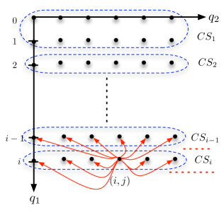
Figure 3: Case (ii) in the proof of Theorem 9: state $(i,j)$ can only transit to the states in the $CS_{i}$ and $CS_{i-1}$.

Case (ii): $p^{(1)}_{0}+p^{(1)}_{1}=1$ and $p^{(2)}_{0}+p^{(2)}_{1}<1$. Note that $\tilde{\theta}$ results in a reducible Markov chain. That is, there are several communicating classes as depicted in Fig. 3.

We define the classes $CS_{1}=\{(a,b):a=0,1\text{\,\,and\,\,}b\in\mathbb{N}\cup\{0\}\}$ and $CS_{i}=\{(a,b):a=i,b\in\mathbb{N}\cup\{0\}\}$ for $i\geq 2$. Then each $CS_{i}$ is a communicating class under policy $\tilde{\theta}$. The states in $CS_{1}$ are positive-recurrent, and each $CS_{i}$ for $i\geq 2$ is a transient class. For $i\geq 2$, let $\overline{C}_{i,j}$ be the expected cost of the passage from state $(i,j)$ (in class $CS_{i}$) to the next class $CS_{i-1}$. Note that state $(i,j)$ has the probability of $p^{(1)}_{0}$ to escape to class $CS_{i-1}$ and $p^{(1)}_{1}$ to remain in class $CS_{i}$. Now $C((i,Q^{(2)}_{t}),1)=C_{T}+C_{H}([i-1]^{+}+[Q^{(2)}_{t}-1]^{+})$. By considering all the possible paths to escape from state $(i,j)$, we can compute $\overline{C}_{i,j}$ as follows:

$$\overline{C}_{i,j}= \mathbb{E}\left[\sum_{k=0}^{\infty}(p^{(1)}_{1})^{k}p^{(1)}_{0}\sum^{k}_{t=0}C((i,Q^{(2)}_{t}),1)|(Q^{(1)}_{0},Q^{(2)}_{0})=(i,j)\right]$$

$$= p^{(1)}_{0}\mathbb{E}\left[\sum^{\infty}_{t=0}C((i,Q^{(2)}_{t}),1)\sum^{\infty}_{k=t}(p^{(1)}_{1})^{k}|(Q^{(1)}_{0},Q^{(2)}_{0})=(i,j)\right]$$

$$= \mathbb{E}\left[\sum^{\infty}_{t=0}(p^{(1)}_{1})^{t}C((i,Q^{(2)}_{t}),1)|(Q^{(1)}_{0},Q^{(2)}_{0})=(i,j)\right].$$

We observe that $\overline{C}_{i,j}$ can be viewed as the total expected $p^{(1)}_{1}$-discounted cost of the system. Following the arguments similar to these in the proof of Proposition 3, we conclude that $\overline{C}_{i,j}<\infty$.

We denote the expected cost of a first passage from state $(i,j)$ to $(k,l)$ by $\overline{C}_{(i,j),(k,l)}.$ Proposition 4 in [19] implies that $\overline{C}_{(1,j),(0,0)}<\infty$ for any $j$, where the intuition is that the expected traveling time from state $(1,j)$ to $(0,0)$ is finite due to the positive recurrence of $CS_{1}$. Let $T_{0}=\min\{t\geq 1:(Q^{(1)}_{t},Q^{(2)}_{t})=(0,0)\}$ and for $i\geq 1$, $T_{i}=\min\{t\geq 1:Q^{(1)}_{t}=i\}$ with the corresponding state $(Q^{(1)}_{T_{i}},Q^{(2)}_{T_{i}})=(i,\tilde{j}_{i})$. Since

$$\overline{C}_{(i,j),(0,0)}=\overline{C}_{i,j}+\sum_{k=1}^{i-2}\overline{C}_{i-k,\tilde{j}_{i-k}}+\overline{C}_{(1,\tilde{j}_{1}),(0,0)},$$

we conclude that $\overline{C}_{(i,j),(0,0)}<\infty$.

Let $\hat{\theta}$, be a policy that always transmits until time slot $T_{0}$ after which the $\alpha$-optimal policy is employed. Then, $V_{\alpha}(i,j)$ can be bounded by

$$V_{\alpha}(i,j)\leq \mathbb{E}_{\hat{\theta}}\left[\sum_{t=0}^{T_{0}-1}\alpha^{t}C(Q_{t},a_{t})|Q_{0}=(i,j)\right]+$$

$$\mathbb{E}_{\hat{\theta}}\left[\sum_{t=T_{0}}^{\infty}\alpha^{t}C(Q_{t},a_{t})|Q_{0}=(i,j)\right]$$

$$\leq \overline{C}_{(i,j),(0,0)}+V_{\alpha}(0,0).$$

We show that condition (iii) of Lemma 7 is satisfied by choosing $M_{i,j}=\overline{C}_{(i,j),(0,0)}$. In particular, it holds that $v_{\alpha}(i,j)=V_{\alpha}(i,j)-V_{\alpha}(0,0)\leq M_{i,j}$ and $M_{i,j}<\infty$. Moreover, $\sum_{k=0}^{\infty}\sum_{l=0}^{\infty}P_{1}\bigl{(}(i,j),(k,l)\bigr{)}M_{k,l}=\sum_{k=0}^{\infty}\sum_{l=0}^{\infty}P_{1}\bigl{(}(i,j),(k,l)\bigr{)}\overline{C}_{(k,l),(0,0)}\leq\overline{C}_{(i,j),(0,0)}<\infty$.

Case (iii): $p^{(i)}_{0}+p^{(i)}_{1}=1$ for $i=1,2$, i.e., Bernoulli arrivals to both queues. Note that in this case $\tilde{\theta}$ also results in a reducible Markov chain. The proof is similar to case (ii) - we define $M_{i,j}=\overline{C}_{(i,j),(0,0)}$, and show that $\overline{C}_{(i,j),(0,0)}$ is finite for this case. ∎

According to Borkar [23], it is possible to find the randomized policy that is closed to the average-optimal by applying linear programming methods for an MDP of a very generic setting, where randomized stationary policies are average-optimal. However, since the average-optimal policy has further been shown in Theorem 9 to be deterministic, in the next section we investigate the structural properties of the average-optimal policy and using a Markov-chain based enumeration to find the average-optimal polity that would be deterministic stationary.

V Structure of the Average-Optimal Policy - Threshold Based

Now that we know the average-optimal policy is stationary and deterministic, the question is how do we find it? If we know that the average-optimal policy satisfies the structural properties, then it is possible to search through the space of stationary deterministic policies and obtain the optimal one. We will study the $\alpha$-optimal policy first and then discuss how to correlate it with the average-optimal policy. Before investigating the general i.i.d. arrival model, we study a special case, namely Bernoulli process. Our objective is to determine the $\alpha$-optimal policy for the Bernoulli arrival process.

Lemma 10.

For the i.i.d. Bernoulli arrival process and the system starting from the empty queues, the $\alpha$-optimal policy is of threshold type. In particular, there exist optimal thresholds $L^{*}_{\alpha,1}$ and $L^{*}_{\alpha,2}$ so that the optimal deterministic action in state $(i,0)$ is to wait if $i\leq L^{*}_{\alpha,1}$, and to transmit without coding if $i>L^{*}_{\alpha,1}$; while in state $(0,j)$ is to wait if $j\leq L^{*}_{\alpha,2}$, and to transmit without coding if $j>L^{*}_{\alpha,2}$.

Proof.

We define

$$\mathcal{V}_{\alpha}(i,0,a)$$

$$= C_{H}([i-a]^{+})+C_{T}a+\alpha\sum_{k,l}P_{a}\bigl{(}(i,0),(k,l)\bigr{)}V_{\alpha}(k,l).$$

Then,

$$V_{\alpha}(i,0)=\min_{a\in\{0,1\}}\mathcal{V}_{\alpha}(i,0,a).$$

Let $L^{*}_{\alpha,1}=\min\{i\in\mathbb{N}\cup\{0\}:\mathcal{V}_{\alpha}(i,0,1)>\mathcal{V}_{\alpha}(i,0,0)\}-1$. Then the optimal stationary and deterministic action (for the total expected $\alpha$-discounted cost) is $a_{t}=0$ for the states $(i,0)$ with $i\leq L^{*}_{\alpha,1}$, and $a_{t}=1$ for the state $(L^{*}_{\alpha,1}+1,0)$. Note that we do not need to define the policy of states $(i,0)$ for $i>L^{*}_{\alpha,1}+1$, since they are not accessible as $(L^{*}_{\alpha,1}+1,0)$ only transits to $(L^{*}_{\alpha,1},0)$, $(L^{*}_{\alpha,1}+1,0)$, $(L^{*}_{\alpha,1},1)$, and $(L^{*}_{\alpha,1}+1,1)$. The similar argument is applicable for the states $(0,j)$. Consequently, there exists a policy of threshold type that is $\alpha$-optimal. ∎

V-A General i.i.d. arrival process

For the i.i.d. Bernoulli arrival process, we have just shown that the $\alpha$-optimal policy is threshold based. Our next objective is to extend this result to any i.i.d. arrival process. We define that $\mathcal{V}_{\alpha}(i,j,a)=C_{H}\left([i-a]^{+}+[j-a]^{+}\right)+C_{T}\cdot a+\alpha\mathbb{E}[V_{\alpha}\left([i-a]^{+}+\mathcal{A}_{1},[j-a]^{+}+\mathcal{A}_{2}\right)]$. Moreover, let $\mathcal{V}_{\alpha,n}(i,j,a)=C_{H}\left([i-a]^{+}+[j-a]^{+}\right)+C_{T}a+\alpha\mathbb{E}[V_{\alpha,n}\left([i-a]^{+}+\mathcal{A}_{1},[j-a]^{+}+\mathcal{A}_{2}\right)]$. Then Eq. (5) can be written as $V_{\alpha}(i,j)=\min_{a\in\{0,1\}}\mathcal{V}_{\alpha}(i,j,a)$, while Eq. (6) can be written as $V_{\alpha,n+1}(i,j)=\min_{a\in\{0,1\}}\mathcal{V}_{\alpha,n}(i,j,a)$. For every discount factor $\alpha$, we want to show that there exists an $\alpha$-optimal policy that is of threshold type. To be precise, let the $\alpha$-optimal policy for the first dimension be $a^{*}_{\alpha,i}=\min{\{a^{\prime}\in\operatornamewithlimits{arg\,min}_{a\in\{0,1\}}\mathcal{V}_{\alpha}(i,0,a)}\}$, and we will show that $a^{*}_{\alpha,i}$ is non-decreasing as $i$ increases, and so is the second dimension. We start with a number of definitions that describe the properties of $V_{\alpha}(i,j)$.

Definition 11 ([20], Submodularity).

A function $f:(\mathbb{N}\cup\{0\})^{2}\rightarrow\mathbb{R}$ is submodular if for all $i,j\in\mathbb{N}\cup\{0\}$

$$f(i,j)+f(i+1,j+1)\leq f(i+1,j)+f(i,j+1).$$

Definition 12 ($\mathcal{K}$-Convexity).

A function $f:(\mathbb{N}\cup\{0\})^{2}\rightarrow\mathbb{R}$ is $\mathcal{K}$-convex (where $\mathcal{K}\in\mathbb{N}$) if for every $i,j\in\mathbb{N}\cup\{0\}$

$$f(i+\mathcal{K},j)-f(i,j)\leq f(i+\mathcal{K}+1,j)-f(i+1,j);$$

$$f(i,j+\mathcal{K})-f(i,j)\leq f(i,j+\mathcal{K}+1)-f(i,j+1).$$

Definition 13 ($\mathcal{K}$-Subconvexity).

A function $f:(\mathbb{N}\cup\{0\})^{2}\rightarrow\mathbb{R}$ is $\mathcal{K}$-subconvex (where $\mathcal{K}\in\mathbb{N}$) if for all $i,j\in\mathbb{N}\cup\{0\}$

$$f(i+\mathcal{K},j+\mathcal{K})-f(i,j)\leq f(i+\mathcal{K}+1,j+\mathcal{K})-f(i+1,j);$$

$$f(i+\mathcal{K},j+\mathcal{K})-f(i,j)\leq f(i+\mathcal{K},j+\mathcal{K}+1)-f(i,j+1).$$

Remark 14.

If a function $f:(\mathbb{N}\cup\{0\})^{2}\rightarrow\mathbb{R}$ is submodular and $\mathcal{K}$-subconvex, then it is $\mathcal{K}$-convex, and for every $r\in\mathbb{N}$ with $1\leq r<\mathcal{K}$,

$$f(i+\mathcal{K},j+r)-f(i,j)\leq f(i+\mathcal{K}+1,j+r)-f(i+1,j);$$

$$f(i+r,j+\mathcal{K})-f(i,j)\leq f(i+r,j+\mathcal{K}+1)-f(i,j+1).$$

For simplicity, we will ignore $\mathcal{K}$ in definitions 12 and 13 when $\mathcal{K}=1$. We will show in Subsection V-C that $V_{\alpha}(i,j)$ is non-decreasing, submodular, and subconvex, that result in the threshold base of $\alpha$-optimal policy. Note that the definition of $\mathcal{K}$-Convexity (Definition 12) is dimension-wise, which is different from the definition of convexity for the continuous function in two dimensions.

V-B Proof overview

Before the technical proofs in Subsection V-C, in this subsection, we overview why submodularity and subconvexity of $V_{\alpha}(i,j)$ lead to the $\alpha$-optimality of the threshold based policy.

• To show that $\alpha$-optimal policy is monotonic w.r.t. state $(i,0)$, it suffices to show that $\mathcal{V}_{\alpha}(i,0,1)-\mathcal{V}_{\alpha}(i,0,0)$ is a non-increasing function w.r.t. $i$: Suppose it is true that $\mathcal{V}_{\alpha}(i+1,0,1)-\mathcal{V}_{\alpha}(i+1,0,0)\leq\mathcal{V}_{\alpha}(i,0,1)-\mathcal{V}_{\alpha}(i,0,0)$. We observe that if the $\alpha$-optimal policy for state $(i,0)$ is $a^{*}_{\alpha,i}=1$, i.e., $\mathcal{V}_{\alpha}(i,0,1)-\mathcal{V}_{\alpha}(i,0,0)\leq 0$, then the $\alpha$-optimal policy for state $(i+1,0)$ is also $a^{*}_{\alpha,i+1}=1$. Similarly, if the $\alpha$-optimal policy for state $(i+1,0)$ is $a^{*}_{\alpha,i+1}=0$ then the $\alpha$-optimal policy for state $(i,0)$ is $a^{*}_{\alpha,i}=0$.

• In oder to prove that $\mathcal{V}_{\alpha}(i,0,1)-\mathcal{V}_{\alpha}(i,0,0)$ is non-increasing, it is sufficient to show that $V_{\alpha}(i,j)$ is convex: When $i\geq 1$, the claim is true since

  $$\mathcal{V}_{\alpha}(i,0,1)-\mathcal{V}_{\alpha}(i,0,0)$$

  $$= C_{T}-C_{H}+\alpha\mathbb{E}[V_{\alpha}(i-1+\mathcal{A}_{1},\mathcal{A}_{2})-V_{\alpha}(i+\mathcal{A}_{1},\mathcal{A}_{2})].$$

• Similarly, to show that $\alpha$-optimal policy of state $(i,j)$ is monotonic w.r.t. $i$ for fixed $j$ and vice versa, it suffices to show that $V_{\alpha}(i,j)$ is subconvex: When $i,j\geq 1$, we observe that

  $$\mathcal{V}_{\alpha}(i,j,1)-\mathcal{V}_{\alpha}(i,j,0)$$

  $$= C_{t}-2C_{h}+\alpha\mathbb{E}[V_{\alpha}(i-1+\mathcal{A}_{1},j-1+\mathcal{A}_{2})-$$

  $$\hskip 65.44142ptV_{\alpha}(i+\mathcal{A}_{1},j+\mathcal{A}_{2})].$$

• To show $V_{\alpha}(i,j)$ is convex and subconvex, we need $V_{\alpha}(i,j)$ is submodular: We intend to prove the convexity and subconvexity of $V_{\alpha}(i,j)$ by induction, which will require the relation between $V_{\alpha}(i,j)+V_{\alpha}(i+1,j+1)$ and $V_{\alpha}(i+1,j)+V_{\alpha}(i,j+1)$. There will be two choices: (i) $V_{\alpha}(i,j)+V_{\alpha}(i+1,j+1)\leq V_{\alpha}(i+1,j)+V_{\alpha}(i,j+1)$, or (ii) $V_{\alpha}(i,j)+V_{\alpha}(i+1,j+1)\geq V_{\alpha}(i+1,j)+V_{\alpha}(i,j+1)$. We might assume that $V_{\alpha}(i,j)$ satisfies (i). Then (i) and the subconvexity of $V_{\alpha}(i,j)$ implies the convexity of $V_{\alpha}(i,j)$. In the contrary, the convexity of $V_{\alpha}(i,j)$ and (ii) lead to the subconvexity of $V_{\alpha}(i,j)$. In other words, both choices are possible since they do not violate the convexity and subconvexity of $V_{\alpha}(i,j)$. Now we are going to argue that the choice (ii) is wrong. Suppose the actions of $\alpha$-optimal policy for the states $(i,j)$, $(i+1,j)$, $(i,j+1)$, $(i+1,j+1)$ are $0,0,1,1$ respectively. If the choice (ii) is true, then when $i\geq 1$, we have

  $$C_{H}(i+j)+\mathbb{E}[V_{\alpha,n}(i+\mathcal{A}_{1},j+\mathcal{A}_{2})]+$$

  $$C_{T}+C_{H}(i+j)+\mathbb{E}[V_{\alpha,n}(i+\mathcal{A}_{1},j+\mathcal{A}_{2})]$$

  $$\geq C_{H}(i+1+j)+\mathbb{E}[V_{\alpha,n}(i+1+\mathcal{A}_{1},j+\mathcal{A}_{2})]+$$

  $$C_{T}+C_{H}(i-1+j)+\mathbb{E}[V_{\alpha,n}(i-1+\mathcal{A}_{1},j+\mathcal{A}_{2})].$$

  By simplifying the above inequality, we can observe the contradiction to the fact that $V_{\alpha,n}(i,j)$ is convex. Therefore, $V_{\alpha}(i,j)$ is submodular.

So far, we know that if we show $V_{\alpha}(i,j)$ is submodular and subconvex, then the $\alpha$-optimal policy of state $(i,j)$ is non-decreasing separately in the direction of $i$ and $j$ (i.e., threshold type). Next, we briefly discuss how Lemmas 15-18 and Theorem 19 in the next subsection work together. Theorem 19 states that the $\alpha$-optimal policy is of threshold type, with the proof of induction on $n$ in Eq. (6). First, we observe that $V_{\alpha,0}(i,j)$ is non-decreasing, submodular, and subconvex. Second, based on Lemma 15 and Corollary 16, $\min\{a^{\prime}\in\operatornamewithlimits{arg\,min}_{a\in\{0,1\}}\mathcal{V}_{\alpha,0}(i,j,a)\}$ is non-decreasing w.r.t. $i$ for fixed $j$, and vice versa. Third, according to Lemmas 6, 17, and 18, we know that $V_{\alpha,1}(i,j)$ is non-decreasing, submodular, and subconvex. Therefore, as $n$ goes to infinity, we conclude that $V_{\alpha}(i,j)$ is non-decreasing, submodular, and subconvex, as well as $\min\{a^{\prime}\in\operatornamewithlimits{arg\,min}_{a\in\{0,1\}}\mathcal{V}_{\alpha}(i,j,a)\}$ is non-decreasing w.r.t. $i$ for fixed $j$, and vice versa.

V-C Main results and proofs

Lemma 15.

Given $0<\alpha<1$ and $n\in\mathbb{N}\cup\{0\}$. If $V_{\alpha,n}(i,j)$ is non-decreasing, submodular, and subconvex, then $\mathcal{V}_{\alpha,n}(i,j,a)$ is submodular for $i$ and $a$ when $j$ is fixed, and so is for $j$ and $a$ when $i$ is fixed.

Proof.

We define $\Delta\mathcal{V}_{\alpha,n}(i,j)=\mathcal{V}_{\alpha,n}(i,j,1)-\mathcal{V}_{\alpha,n}(i,j,0)$. We claim that $\Delta\mathcal{V}_{\alpha,n}(i,j)$ is non-increasing, i.e., $\Delta\mathcal{V}_{\alpha,n}(i,j)$ is a non-increasing function w.r.t. $i$ while $j$ is fixed, and vice versa (we will focus on the former part). Notice that

$$\Delta\mathcal{V}_{\alpha,n}(i,j) = C_{H}([i-1]^{+}+(j-1)^{+})+C_{T}+$$

$$\alpha\mathbb{E}[V_{\alpha,n}([i-1]^{+}+\mathcal{A}_{1},[j-1]^{+}+\mathcal{A}_{2})]-$$

$$C_{H}(i+j)-\alpha\mathbb{E}[V_{\alpha,n}(i+\mathcal{A}_{1},j+\mathcal{A}_{2})].$$

To be precise, when $i\geq 1$,

$$\Delta\mathcal{V}_{\alpha,n}(i,j)= C_{T}-2C_{H}+\alpha\mathbb{E}[V_{\alpha,n}(i-1+\mathcal{A}_{1},j-1+\mathcal{A}_{2})-$$

$$V_{\alpha,n}(i+\mathcal{A}_{1},j+\mathcal{A}_{2})]\,\,\,\text{for}\,\,j\geq 1;$$ (8)

$$\Delta\mathcal{V}_{\alpha,n}(i,j)= C_{T}-C_{H}+\alpha\mathbb{E}[V_{\alpha,n}(i-1+\mathcal{A}_{1},\mathcal{A}_{2})-$$

$$V_{\alpha,n}(i+\mathcal{A}_{1},\mathcal{A}_{2})]\,\,\,\text{for}\,\,j=0.$$ (9)

Because of the subconvexity of $V_{\alpha,n}(i,j)$ in Eq. (8), when $i\geq 1$ and $j\geq 1$, $\Delta\mathcal{V}_{\alpha,n}(i,j)$ does not increase as $i$ increases. The same is for $i\geq 1$ and $j=0$ in Eq. (9) due to the convexity of $V_{\alpha,n}(i,j)$.

We proceed to establish the boundary conditions. When $j\geq 1$,

$$\Delta\mathcal{V}_{\alpha,n}(1,j) = C_{T}-2C_{H}+\alpha\mathbb{E}[V_{\alpha,n}(\mathcal{A}_{1},j-1+\mathcal{A}_{2})-$$

$$\hskip 71.13188ptV_{\alpha,n}(1+\mathcal{A}_{1},j+\mathcal{A}_{2})];$$

$$\Delta\mathcal{V}_{\alpha,n}(0,j) = C_{T}-C_{H}+\alpha\mathbb{E}[V_{\alpha,n}(\mathcal{A}_{1},j-1+\mathcal{A}_{2})-$$

$$\hskip 71.13188ptV_{\alpha,n}(\mathcal{A}_{1},j+\mathcal{A}_{2})].$$

Note that $\mathbb{E}[V_{\alpha,n}(1+\mathcal{A}_{1},j+\mathcal{A}_{2})]\geq\mathbb{E}[V_{\alpha,n}(\mathcal{A}_{1},j+\mathcal{A}_{2})]$ according to non-decreasing $V_{\alpha,n}(i,j)$ and then $\Delta\mathcal{V}_{\alpha,n}(1,j)\leq\Delta\mathcal{V}_{\alpha,n}(0,j)$ when $j\geq 1$. Finally, when $j=0$ we have

$$\Delta\mathcal{V}_{\alpha,n}(1,0) = C_{T}-C_{H}+\alpha\mathbb{E}[V_{\alpha,n}(\mathcal{A}_{1},\mathcal{A}_{2})-$$

$$\hskip 71.13188ptV_{\alpha,n}(1+\mathcal{A}_{1},\mathcal{A}_{2})];$$

$$\Delta\mathcal{V}_{\alpha,n}(0,0) = C_{T}.$$

Here, $\Delta\mathcal{V}_{\alpha,n}(1,0)\leq\Delta\mathcal{V}_{\alpha,n}(0,0)$ since $\mathbb{E}[V_{\alpha,n}(\mathcal{A}_{1},\mathcal{A}_{2})-V_{\alpha,n}(1+\mathcal{A}_{1},\mathcal{A}_{2})]\leq 0$ as $V_{\alpha,n}(i,j)$ is non-decreasing. Consequently, $\Delta\mathcal{V}_{\alpha,n}(i,j)$ is a non-increasing function w.r.t. $i$ while $j$ is fixed. ∎

Submodularity of $\mathcal{V}_{\alpha,n}(i,j,a)$ implies the monotonicity of the optimal minimizing policy [12, Lemma 4.7.1] as described in the following Corollary. This property will simplify the proofs of Lemmas 17 and 18.

Corollary 16.

Given $0<\alpha<1$ and $n\in\mathbb{N}\cup\{0\}$. If $V_{\alpha,n}(i,j)$ is non-decreasing, submodular, and subconvex, then $\min\{a^{\prime}\in\operatornamewithlimits{arg\,min}_{a\in\{0,1\}}\mathcal{V}_{\alpha,n}(i,j,a)\}$ is non-decreasing w.r.t. $i$ for fixed $j$, and vice versa.

Lemma 17.

Given $0<\alpha<1$ and $n\in\mathbb{N}\cup\{0\}$. If $V_{\alpha,n}(i,j)$ is non-decreasing, submodular, and subconvex, then $V_{\alpha,n+1}(i,j)$ is submodular.

Proof.

We intend to show that $V_{\alpha,n+1}(i+1,j+1)-V_{\alpha,n+1}(i+1,j)\leq V_{\alpha,n+1}(i,j+1)-V_{\alpha,n+1}(i,j)$ for all $i,j\in\mathbb{N}\cup\{0\}$. According to Corollary 16, only 6 cases of $(a^{*}_{i,j},a^{*}_{i+1,j},a^{*}_{i,j+1},a^{*}_{i+1,j+1})$ are considered, where $a^{*}_{i,j}=\min\{a^{\prime}\in\operatornamewithlimits{arg\,min}_{a\in\{0,1\}}\mathcal{V}_{\alpha,n}(i,j,a)\}$.

Case (i): if $(a^{*}_{i,j},a^{*}_{i+1,j},a^{*}_{i,j+1},a^{*}_{i+1,j+1})=(1,1,1,1)$, we claim that

$$\mathbb{E}[V_{\alpha,n}(i+\mathcal{A}_{1},j+\mathcal{A}_{2})-V_{\alpha,n}(i+\mathcal{A}_{1},[j-1]^{+}+\mathcal{A}_{2})]$$

$$\leq \mathbb{E}[V_{\alpha,n}([i-1]^{+}+\mathcal{A}_{1},j+\mathcal{A}_{2})-$$

$$\hskip 11.38092ptV_{\alpha,n}([i-1]^{+}+\mathcal{A}_{1},[j-1]^{+}+\mathcal{A}_{2})].$$

When $i,j\neq 0$, it is true according to submodularity of $V_{\alpha,n}(i,j)$. Otherwise, both sides of the inequality are 0.

Case (ii): if $(a^{*}_{i,j},a^{*}_{i+1,j},a^{*}_{i,j+1},a^{*}_{i+1,j+1})=(0,0,0,0)$, we claim that

$$\mathbb{E}[V_{\alpha,n}(i+1+\mathcal{A}_{1},j+1+\mathcal{A}_{2})-V_{\alpha,n}(i+1+\mathcal{A}_{1},j+\mathcal{A}_{2})]$$

$$\leq \mathbb{E}[V_{\alpha,n}(i+\mathcal{A}_{1},j+1+\mathcal{A}_{2})-V_{\alpha,n}(i+\mathcal{A}_{1},j+\mathcal{A}_{2})].$$

This is obvious from the submodularity of $V_{\alpha,n}(i,j)$.

Case (iii): if $(a^{*}_{i,j},a^{*}_{i+1,j},a^{*}_{i,j+1},a^{*}_{i+1,j+1})=(0,0,0,1)$, we claim that

$$C_{T}-C_{H}+\alpha\mathbb{E}[V_{\alpha,n}(i+\mathcal{A}_{1},j+\mathcal{A}_{2})-$$

$$\hskip 68.28644ptV_{\alpha,n}(i+1+\mathcal{A}_{1},j+\mathcal{A}_{2})]$$

$$\leq C_{H}+\alpha\mathbb{E}[V_{\alpha,n}(i+\mathcal{A}_{1},j+1+\mathcal{A}_{2})-$$

$$\hskip 42.67912ptV_{\alpha,n}(i+\mathcal{A}_{1},j+\mathcal{A}_{2})].$$

From the submodularity of $V_{\alpha,n}(i,j)$, it is obtained that

$$V_{\alpha,n}(i,j)-V_{\alpha,n}(i+1,j)+V_{\alpha,n}(i,j)-V_{\alpha,n}(i,j+1)$$

$$\leq V_{\alpha,n}(i,j)-V_{\alpha,n}(i+1,j)+V_{\alpha,n}(i+1,j)-$$

$$V_{\alpha,n}(i+1,j+1)$$

$$= V_{\alpha,n}(i,j)-V_{\alpha,n}(i+1,j+1).$$

Since $a^{*}_{i+1,j+1}=1$, we have $\Delta\mathcal{V}_{\alpha,n}(i+1,j+1)\leq 0$, i.e.,

$$C_{T}-2C_{H}+\alpha\mathbb{E}[V_{\alpha,n}(i+\mathcal{A}_{1},j+\mathcal{A}_{2})-$$

$$\hskip 73.97733ptV_{\alpha,n}(i+1+\mathcal{A}_{1},j+1+\mathcal{A}_{2})]\leq 0.$$

The claim follows from the following equation:

$$C_{T}-2C_{H}+\alpha\mathbb{E}[V_{\alpha,n}(i+\mathcal{A}_{1},j+\mathcal{A}_{2})-$$

$$\hskip 71.13188ptV_{\alpha,n}(i+1+\mathcal{A}_{1},j+\mathcal{A}_{2})+$$

$$\hskip 71.13188ptV_{n}(i+\mathcal{A}_{1},j+\mathcal{A}_{2})-$$

$$\hskip 71.13188ptV_{\alpha,n}(i+\mathcal{A}_{1},j+1+\mathcal{A}_{2})]$$

$$\leq \Delta\mathcal{V}_{\alpha,n}(i+1,j+1)\leq 0.$$

Case (iv): if $(a^{*}_{i,j},a^{*}_{i+1,j},a^{*}_{i,j+1},a^{*}_{i+1,j+1})=(0,0,1,1)$, we claim that

$$-C_{H}+\alpha\mathbb{E}[V_{\alpha,n}(i+\mathcal{A}_{1},j+\mathcal{A}_{2})-$$

$$\hskip 48.36958ptV_{\alpha,n}(i+1+\mathcal{A}_{1},j+\mathcal{A}_{2})]$$

$$\leq C_{H}([i-1]^{+}-i)+\alpha\mathbb{E}[V_{\alpha,n}([i-1]^{+}+\mathcal{A}_{1},j+\mathcal{A}_{2})-$$

$$\hskip 99.58464ptV_{\alpha,n}(i+\mathcal{A}_{1},j+\mathcal{A}_{2})]$$

When $i\neq 0$, it is satisfied because $V_{\alpha,n}(i,j)$ is convex. Otherwise, it is true since $V_{\alpha,n}(i,j)$ is non-decreasing.

Case (v): if $(a^{*}_{i,j},a^{*}_{i+1,j},a^{*}_{i,j+1},a^{*}_{i+1,j+1})=(0,1,0,1)$, we claim that

$$C_{H}(j-[j-1]^{+})+\alpha\mathbb{E}[V_{\alpha,n}(i+\mathcal{A}_{1},j+\mathcal{A}_{2})-$$

$$\hskip 99.58464ptV_{\alpha,n}(i+\mathcal{A}_{1},[j-1]^{+}+\mathcal{A}_{2})]$$

$$\leq C_{H}+\alpha\mathbb{E}[V_{\alpha,n}(i+\mathcal{A}_{1},j+1+\mathcal{A}_{2})-V_{\alpha,n}(i+\mathcal{A}_{1},j+\mathcal{A}_{2})].$$

When $j\neq 0$, it holds since $V_{\alpha,n}(i,j)$ is convex. It is true for other cases because of the non-decreasing $V_{\alpha,n}(i,j)$.

Case (vi): if $(a^{*}_{i,j},a^{*}_{i+1,j},a^{*}_{i,j+1},a^{*}_{i+1,j+1})=(0,1,1,1)$, we claim that

$$C_{H}(j-[j-1]^{+})+\alpha\mathbb{E}[V_{\alpha,n}(i+\mathcal{A}_{1},j+\mathcal{A}_{2})-$$

$$\hskip 102.43008ptV_{\alpha,n}(i+\mathcal{A}_{1},[j-1]^{+}+\mathcal{A}_{2})]$$

$$\leq C_{T}+C_{H}([i-1]^{+}-i)+\alpha\mathbb{E}[V_{\alpha,n}([i-1]^{+}+\mathcal{A}_{1},j+\mathcal{A}_{2})-$$

$$\hskip 125.19194ptV_{\alpha,n}(i+\mathcal{A}_{1},j+\mathcal{A}_{2})].$$

Based on the submodularity of $V_{\alpha,n}(i,j)$, we have

$$V_{\alpha,n}([i-1]^{+},j)-V_{\alpha,n}(i,j)+V_{\alpha,n}(i,[j-1]^{+})-V_{\alpha,n}(i,j)$$

$$\geq V_{\alpha,n}([i-1]^{+},[j-1]^{+})-V_{\alpha,n}(i,[j-1]^{+})+$$

$$V_{\alpha,n}(i,[j-1]^{+})-V_{\alpha,n}(i,j)$$

$$= V_{\alpha,n}([i-1]^{+},[j-1]^{+})-V_{\alpha,n}(i,j).$$

It is noted that $a^{*}_{i,j}=0$ and hence $\Delta\mathcal{V}_{\alpha,n}(i,j)\geq 0$, i.e.,

$$C_{T}+C_{H}([i-1]^{+}+[j-1]^{+}-i-j)+$$

$$\alpha\mathbb{E}[V_{\alpha,n}([i-1]^{+}+\mathcal{A}_{1},[j-1]^{+}+\mathcal{A}_{1})-$$

$$V_{\alpha,n}(i+\mathcal{A}_{1},j+\mathcal{A}_{1})]\geq 0.$$

Therefore, it can be concluded that

$$C_{T}+C_{H}([i-1]^{+}+[j-1]^{+}-i-j)+$$

$$\alpha\mathbb{E}[V_{\alpha,n}([i-1]^{+}+\mathcal{A}_{1},j+\mathcal{A}_{2})-$$

$$\hskip 14.22636ptV_{\alpha,n}(i+\mathcal{A}_{1},j+\mathcal{A}_{2})+V_{\alpha,n}(i+\mathcal{A}_{1},[j-1]^{+}+\mathcal{A}_{2})-$$

$$\hskip 14.22636ptV_{\alpha,n}(i+\mathcal{A}_{1},j+\mathcal{A}_{2})]$$

$$\geq \Delta\mathcal{V}_{\alpha,n}(i,j)\geq 0.$$

∎

Lemma 18.

Given $0<\alpha<1$ and $n\in\mathbb{N}\cup\{0\}$. If $V_{\alpha,n}(i,j)$ is non-decreasing, submodular, and subconvex, then $V_{\alpha,n+1}(i,j)$ is subconvex.

Proof.

We want to show that $V_{\alpha,n+1}(i+1,j+1)-V_{\alpha,n+1}(i,j)\leq V_{\alpha,n+1}(i+2,j+1)-V_{\alpha,n+1}(i+1,j)$ for all $i$ and $j$. There will be 5 cases of $(a^{*}_{i,j},a^{*}_{i+1,j},a^{*}_{i+1,j+1},a^{*}_{i+2,j+1})$ that need to be considered.

Case (i): if $(a^{*}_{i,j},a^{*}_{i+1,j},a^{*}_{i+1,j+1},a^{*}_{i+2,j+1})=(1,1,1,1)$, we claim that

$$C_{H}(i-[i-1]^{+})+\alpha\mathbb{E}[V_{\alpha,n}(i+\mathcal{A}_{1},j+\mathcal{A}_{2})-$$

$$\hskip 102.43008ptV_{\alpha,n}([i-1]^{+}+\mathcal{A}_{1},[j-1]^{+}+\mathcal{A}_{2})]$$

$$\leq C_{H}+\alpha\mathbb{E}[V_{\alpha,n}(i+1+\mathcal{A}_{1},j+\mathcal{A}_{2})-$$

$$\hskip 45.52458ptV_{\alpha,n}(i+\mathcal{A}_{1},[j-1]^{+}+\mathcal{A}_{2})].$$

When $i,j\neq 0$, it is true according to the subconvexity of $V_{\alpha,n}(i,j)$. The argument is satisfied for $i=0,j\neq 0$ due to the the non-decreasing $V_{\alpha,n}(i,j)$, and for the case $i\neq 0,j=0$ due to the convexity of $V_{\alpha,n}(i,j)$. Otherwise, it holds according to the non-decreasing property.

Case (ii): if $(a^{*}_{i,j},a^{*}_{i+1,j},a^{*}_{i+1,j+1},a^{*}_{i+2,j+1})=(0,0,0,0)$, we claim that

$$\mathbb{E}[V_{\alpha,n}(i+1+\mathcal{A}_{1},j+1+\mathcal{A}_{2})-V_{\alpha,n}(i+\mathcal{A}_{1},j+\mathcal{A}_{2})]$$

$$\leq \mathbb{E}[V_{\alpha,n}(i+2+\mathcal{A}_{1},j+1+\mathcal{A}_{2})-$$

$$\hskip 8.5359ptV_{\alpha,n}(i+1+\mathcal{A}_{1},j+\mathcal{A}_{2})].$$

The above results from the subconvexity of $V_{\alpha,n}(i,j)$.

Case (iii): if $(a^{*}_{i,j},a^{*}_{i+1,j},a^{*}_{i+1,j+1},a^{*}_{i+2,j+1})=(0,0,0,1)$, we claim that

$$2C_{H}+\alpha\mathbb{E}[V_{\alpha,n}(i+1+\mathcal{A}_{1},j+1+\mathcal{A}_{2})-$$

$$\hskip 45.52458ptV_{\alpha,n}(i+\mathcal{A}_{1},j+\mathcal{A}_{2})]\leq C_{T}.$$

Since $a^{*}_{i+1,j+1}=0$, we have $\Delta\mathcal{V}_{\alpha,n}(i+1,j+1)\geq 0$, i.e.,

$$C_{T}-2C_{H}+\alpha\mathbb{E}[V_{\alpha,n}(i+\mathcal{A}_{1},j+\mathcal{A}_{2})-$$

$$\hskip 71.13188ptV_{\alpha,n}(i+1+\mathcal{A}_{1},j+1+\mathcal{A}_{2})]\geq 0.$$

Hence the claim is verified.

Case (iv): if $(a^{*}_{i,j},a^{*}_{i+1,j},a^{*}_{i+1,j+1},a^{*}_{i+2,j+1})=(0,0,1,1)$, it is trivial since the both $V_{\alpha,n+1}(i+1,j+1)-V_{\alpha,n+1}(i,j)$ and $V_{\alpha,n+1}(i+2,j+1)-V_{\alpha,n+1}(i+1,j)$ are zeros.

Case (v): if $(a^{*}_{i,j},a^{*}_{i+1,j},a^{*}_{i+1,j+1},a^{*}_{i+2,j+1})=(0,1,1,1)$, we claim that

$$C_{T} \leq C_{H}(1+j-[j-1]^{+})+$$

$$\alpha\mathbb{E}[V_{\alpha,n}(i+1+\mathcal{A}_{1},j+\mathcal{A}_{2})-$$

$$\hskip 14.22636ptV_{\alpha,n}(i+\mathcal{A}_{1},[j-1]^{+}+\mathcal{A}_{2})].$$

Notice that $a^{*}_{i+1,j}=1$, so $\Delta\mathcal{V}_{\alpha,n}(i+1,j)\leq 0$, i.e.,

$$C_{T}-C_{H}(1+j-[j-1]^{+})+$$

$$\alpha\mathbb{E}[V_{\alpha,n}(i+\mathcal{A}_{1},[j-1]^{+}+\mathcal{A}_{2})-$$

$$\hskip 14.22636ptV_{\alpha,n}(i+1+\mathcal{A}_{1},j+\mathcal{A}_{2})]\leq 0.$$

∎

Based on the properties of $V_{\alpha}(i,j)$, we are ready to state the optimality of the threshold type policy in terms of the total expected discounted cost.

Theorem 19.

For the MDP$\{(Q_{t},a_{t}),t\geq 0\}$ with any i.i.d. arrival processes to both queues, there exists an $\alpha$-optimal policy that is of threshold type. Given $Q^{(2)}_{t}$, the $\alpha$-optimal policy is monotone w.r.t. $Q^{(1)}_{t}$, and vice versa.

Proof.

We prove by induction. $V_{\alpha,0}(i,j)=0$ is non-decreasing, submodular, and subconvex, that leads to the non-decreasing $\min\{a^{\prime}\in\operatornamewithlimits{arg\,min}_{a\in\{0,1\}}\mathcal{V}_{\alpha,0}(i,j,a)\}$ based on Corollary 16. These properties propagate as $n$ goes to infinity according to lemmas 6, 17, 18, and Corollary 16. ∎

Thus far, the $\alpha$-optimal policy is characterized. A useful relation between the average-optimal policy and the $\alpha$-optimal policy is described in the following lemma.

Lemma 20 ([19], Lemma and Theorem (i)).

Consider MDP$\{(Q_{t},a_{t}),t\geq 0\}$. Let $\{\alpha_{n}\}$ converging to 1 be any sequence of discount factors associated with the $\alpha$-optimal policy $\{\theta_{\alpha_{n}}(i,j)\}$. There exists a subsequence $\{\beta_{n}\}$ and a stationary policy $\theta^{*}(i,j)$ that is the limit point of $\{\theta_{\beta_{n}}(i,j)\}$. If the three conditions in Lemma 7 are satisfied, $\theta^{*}(i,j)$ is the average-optimal policy for Eq. (2).

Theorem 21.

Consider any i.i.d. arrival processes to both queues. For the MDP$\{(Q_{t},a_{t}),t\geq 0\}$, the average-optimal policy is of threshold type. There exist the optimal thresholds $L^{*}_{1}$ and $L^{*}_{2}$ so that the optimal deterministic action in states $(i,0)$ is to wait if $i\leq L^{*}_{1}$, and to transmit without coding if $i>L^{*}_{1}$; while in state $(0,j)$ is to wait if $j\leq L^{*}_{2}$, and to transmit without coding if $j>L^{*}_{2}$.

Proof.

Let $(\tilde{i},0)$ be any state which average-optimal policy is to transmit, i.e., $\theta^{*}(\tilde{i},0)=1$ in Lemma 20. Since there is a sequence of discount factors $\{\beta_{n}\}$ such that $\theta_{\beta_{n}}(i,j)\rightarrow\theta^{*}(i,j)$, then there exists $N>0$ so that $\theta_{\beta_{n}}(\tilde{i},0)=1$ for all $n\geq N$. Due to the monotonicity of $\alpha$-optimal policy in Theorem 19, $\theta_{\beta_{n}}(i,0)=1$ for all $i\geq\tilde{i}$ and $n\geq N$. Therefore, $\theta^{*}(i,0)=1$ for all $i\geq\tilde{i}$. To conclude, the average-optimal policy is of threshold type. ∎

VI Obtaining the Optimal Deterministic Stationary Policy

We have shown in the previous sections that the average-optimal policy is stationary, deterministic and of threshold type, so we only need to consider the subset of deterministic stationary policies. Given the thresholds of the both queues, the MDP is reduced to a Markov chain. The next step is to find the optimal threshold. First note that the condition $\mathbb{E}[\mathcal{A}_{i}]<1$ might not be sufficient for the stability of the queues since the threshold based policy leads to an average service rate lower than 1 packet per time slot. In the following theorem, we claim that the conditions $\mathbb{E}[\mathcal{A}_{i}^{2}]<\infty$ and $\mathbb{E}[\mathcal{A}_{i}]<1$ for $i=1,2$ are enough for the stability of the queues.

Theorem 22.

For the MDP$\{(Q_{t},a_{t}),t\geq 0\}$ with $\mathbb{E}[\mathcal{A}_{i}^{2}]<\infty$ and $\mathbb{E}[\mathcal{A}_{i}]<1$ for $i=1,2$. The reduced Markov chain from applying the stationary and deterministic threshold based policy to MDP is positive recurrent, i.e., the stationary distribution exists.

Proof.

The proof is based on Foster-Lyapunov theorem [24] associated with the Lyapunov function $\mathcal{L}(x,y)=x^{2}+y^{2}$. Notice that

$$Q^{(i)}_{t+1} = [Q^{(i)}_{t}-a_{t}]^{+}+\mathcal{A}_{i}$$

$$= Q^{(i)}_{t}-a_{t}+U^{(i)}_{t}+\mathcal{A}_{i},$$

where

$$U^{(i)}_{t}=\left\{\begin{array}[]{ll}0&\text{if\,\,}Q^{(i)}_{t}-a_{t}\geq 0\\ 1&\text{if\,\,}Q^{(i)}_{t}-a_{t}=-1.\\ \end{array}\right.$$

Then it can be observed that

$$\mathbb{E}\left[\mathcal{L}(Q^{(1)}_{t+1},Q^{(2)}_{t+1})-\mathcal{L}(Q^{(1)}_{t},Q^{(2)}_{t})|Q^{(1)}_{t}=x,Q^{(2)}_{t}=y\right]$$

$$= \mathbb{E}\left[\sum^{2}_{i=1}(Q^{(i)}_{t}-a_{t}+U^{(i)}_{t}+\mathcal{A}_{i})^{2}|Q^{(1)}_{t}=x,Q^{(2)}_{t}=y\right]-$$

$$(x^{2}+y^{2})$$

$$= \sum^{2}_{i=1}\mathbb{E}\left[(Q^{(i)}_{t}-a_{t}+\mathcal{A}_{i})^{2}|Q^{(1)}_{t}=x,Q^{(2)}_{t}=y\right]+$$

$$\sum^{2}_{i=1}\mathbb{E}\left[(U^{(i)}_{t})^{2}|Q^{(1)}_{t}=x,Q^{(2)}_{t}=y\right]+$$

$$\sum^{2}_{i=1}\mathbb{E}\left[2U^{(i)}_{t}(Q^{(i)}_{t}-a_{t}+\mathcal{A}_{i})|Q^{(1)}_{t}=x,Q^{(2)}_{t}=y\right]-$$

$$(x^{2}+y^{2})$$

$$\leq \sum^{2}_{i=1}\mathbb{E}\left[(Q^{(i)}_{t}-a_{t}+\mathcal{A}_{i})^{2}|Q^{(1)}_{t}=x,Q^{(2)}_{t}=y\right]+2+$$

$$2\mathbb{E}[\mathcal{A}_{1}]+2\mathbb{E}[\mathcal{A}_{2}]-(x^{2}+y^{2})$$ (11)

$$= 2x\mathbb{E}\left[\mathcal{A}_{1}-a_{t}|Q^{(1)}_{t}=x,Q^{(2)}_{t}=y\right]+$$

$$2y\mathbb{E}\left[\mathcal{A}_{2}-a_{t}|Q^{(1)}_{t}=x,Q^{(2)}_{t}=y\right]+$$

$$\mathbb{E}\left[(\mathcal{A}_{1}-a_{t})^{2}|Q^{(1)}_{t}=x,Q^{(2)}_{t}=y\right]+$$

$$\mathbb{E}\left[(\mathcal{A}_{2}-a_{t})^{2}|Q^{(1)}_{t}=x,Q^{(2)}_{t}=y\right]+$$

$$2\mathbb{E}[\mathcal{A}_{1}]+2\mathbb{E}[\mathcal{A}_{2}]+2$$

$$\leq 2x\mathbb{E}\left[\mathcal{A}_{1}-a_{t}|Q^{(1)}_{t}=x,Q^{(2)}_{t}=y\right]+$$

$$2y\mathbb{E}\left[\mathcal{A}_{2}-a_{t}|Q^{(1)}_{t}=x,Q^{(2)}_{t}=y\right]+$$

$$\mathbb{E}[\mathcal{A}^{2}_{1}]+1+\mathbb{E}[\mathcal{A}^{2}_{2}]+1+2\mathbb{E}[\mathcal{A}_{1}]+2\mathbb{E}[\mathcal{A}_{2}]+2$$ (12)

$$= \mathbb{E}[\mathcal{A}^{2}_{1}]+\mathbb{E}[\mathcal{A}^{2}_{2}]+2\mathbb{E}[\mathcal{A}_{1}]+2\mathbb{E}[\mathcal{A}_{2}]+4+$$

$$\left\{\begin{array}[]{ll}2x(\mathbb{E}[\mathcal{A}_{1}]-1)+2y(\mathbb{E}[\mathcal{A}_{2}]-1)&\text{if}\,\,(x,y)\in\mathcal{B}^{c}\\ 2x\mathbb{E}[\mathcal{A}_{1}]+2y\mathbb{E}[\mathcal{A}_{2}]&\text{if\,\,}(x,y)\in\mathcal{B},\end{array}\right.$$ (15)

where $\mathcal{B}=\{(x,y):(x=0,y\leq L_{2})\text{\,\,or\,\,}(x\leq L_{1},y=0)\}$. The inequality (11) comes from $(U^{(i)}_{t})^{2}\leq 1$ and $(Q^{(i)}_{t}-a_{t})U^{(i)}_{t}\leq 0$, while $\mathbb{E}[a_{t}]\leq 1$ results in Eq. (12). Since $\mathbb{E}[\mathcal{A}_{i}^{2}]<\infty$ and $\mathbb{E}[\mathcal{A}_{i}]<1$ for $i=1,2$, the value in Eq. (15) is negative for $(x,y)\in\mathcal{B}^{c}$ and is bounded for $(x,y)\in\mathcal{B}$. Then the result immediately follows from Foster-Lyapunov theorem. ∎

We realize that if $\mathbb{E}[\mathcal{A}_{i}^{2}]<\infty$ and $\mathbb{E}[\mathcal{A}_{i}]<1$ for $i=1,2$, then there exists a stationary threshold type policy that is average-optimal and can be obtained from the reduced Markov chain. The following theorem gives an example of how to compute the optimal thresholds.

Theorem 23.

Consider the Bernoulli arrival process. The optimal thresholds $L^{*}_{1}$ and $L^{*}_{2}$ are

$$(L^{*}_{1},L^{*}_{2})=\operatornamewithlimits{arg\,min}_{L_{1},L_{2}}C_{T}\mathcal{T}(L_{1},L_{2})+C_{H}\mathcal{H}(L_{1},L_{2}),$$

where

$$\mathcal{T}(L_{1},L_{2}) = p^{(1)}_{1}p^{(2)}_{1}\pi_{0,0}+p^{(2)}_{1}\sum_{i=1}^{L_{1}}\pi_{i,0}+p^{(1)}_{1}\sum_{j=1}^{L_{2}}\pi_{0,j}+$$

$$p^{(1)}_{1}p^{(2)}_{0}\pi_{L_{1},0}+p^{(1)}_{0}p^{(2)}_{1}\pi_{0,L_{2}};$$

$$\mathcal{H}(L_{1},L_{2}) = \sum_{i=1}^{L_{1}}i\pi_{i,0}+\sum_{j=1}^{L_{2}}j\pi_{0,j},$$

for which

$$\pi_{0,0} = \frac{1}{\left(\frac{1-\zeta^{L_{1}+1}}{1-\zeta}\right)+\left(\frac{1-1/\zeta^{L_{2}+1}}{1-1/\zeta}\right)-1};$$

$$\pi_{i,0} = \zeta^{i}\pi_{0,0};$$

$$\pi_{0,j} = \pi_{0,0}/\zeta^{j};$$

$$\zeta = \frac{p^{(1)}_{1}p^{(2)}_{0}}{p^{(1)}_{0}p^{(2)}_{1}}.$$

Proof.

Let $Y^{(i)}_{t}$ be the number of type $i$ packets at the $t^{\text{th}}$ slot after transmission. It is crucial to note that this observation time is different from when the MDP is observed. Then the bivariate stochastic process $\{(Y^{(1)}_{t},Y^{(2)}_{t}),t\geq 0\}$ is a discrete-time Markov chain which state space is smaller than the original MDP, i.e., $(0,0)$, $(1,0)$, $(2,0)$, $\cdots$, $(L_{1},0)$, $(0,1)$, $(0,2)$, $\cdots$, $(0,L_{2})$. Define $\zeta$ as a parameter such that

$$\zeta=\frac{p^{(1)}_{1}p^{(2)}_{0}}{p^{(1)}_{0}p^{(2)}_{1}}.$$

Then, the balance equations for $0<i\leq L_{1}$ and $0<j\leq L_{2}$ are:

$$\pi_{i,0} = \zeta\pi_{i-1,0};$$

$$\zeta\pi_{0,j} = \pi_{0,j-1}.$$

Since $\pi_{0,0}+\sum_{i,j}\pi_{i,0}+\pi_{0,j}=1$, we have

$$\pi_{0,0} = \frac{1}{\left(\frac{1-\zeta^{L_{1}+1}}{1-\zeta}\right)+\left(\frac{1-1/\zeta^{L_{2}+1}}{1-1/\zeta}\right)-1}.$$

The expected number of transmissions per slot is

$$\mathcal{T}(L_{1},L_{2}) = p^{(1)}_{1}p^{(2)}_{1}\pi_{0,0}+p^{(2)}_{1}\sum_{i=1}^{L_{1}}\pi_{i,0}+p^{(1)}_{1}\sum_{j=1}^{L_{2}}\pi_{0,j}+$$

$$p^{(1)}_{1}p^{(2)}_{0}\pi_{L_{1},0}+p^{(1)}_{0}p^{(2)}_{1}\pi_{0,L_{2}}.$$

The average number of packets in the system at the beginning of each slot is

$$\mathcal{H}(L_{1},L_{2})=\sum_{i=1}^{L_{1}}i\pi_{i,0}+\sum_{j=1}^{L_{2}}j\pi_{0,j}.$$

Thus upon minimizing we get the optimal thresholds $L^{*}_{1}$ and $L^{*}_{2}$. ∎

Whenever $C_{H}>0$, it is relatively straightforward to obtain $L^{*}_{1}$ and $L^{*}_{2}$. Since it costs $C_{T}$ to transmit a packet and $C_{H}$ for a packet to wait for a slot, it would be better to transmit a packet than make a packet wait for more than $C_{T}/C_{H}$ slots. Thus $L^{*}_{1}$ and $L^{*}_{2}$ would always be less than $C_{T}/C_{H}$. Hence, by completely enumerating between $0$ and $C_{T}/C_{H}$ for both $L_{1}$ and $L_{2}$, we can obtain $L^{*}_{1}$ and $L^{*}_{2}$. One could perhaps find faster techniques than complete enumeration, but it certainly serves the purpose.

Subsequently, we study a special case, $p^{(1)}_{1}=p^{(2)}_{1}\triangleq p$, in Theorem 23. Then $L_{1}=L_{2}\triangleq L$ as both arrival processes are identical. It can be calculated that $\zeta=1$ and $\pi_{i,j}=1/(2L+1)$ for all $i,j$, and

$$\mathcal{T}(L)=\frac{2pL+2p-p^{2}}{2L+1};$$

$$\mathcal{H}(L)=\frac{L^{2}+L}{2L+1}.$$

Define $\nu=C_{T}/C_{H}$. The optimal threshold is

$$L^{*}(p,\nu)=\operatornamewithlimits{arg\,min}_{L}\frac{\nu(2pL+2p-p^{2})+L+L^{2}}{2L+1}.$$

By taking the derivative, we obtain that $L^{*}=0$ if $\nu<1/(2p-2p^{2})$ and otherwise,

$$L^{*}(p,\nu)=\frac{-1+\sqrt{1-2(1-2\nu p+2\nu p^{2})}}{2}.$$

We can observe that $L^{*}(p,\nu)$ is a concave function w.r.t. $p$. Given $\nu$ fixed, $L^{*}(1/2,\nu)=(\sqrt{\nu-1}-1)/2$ is the largest optimal threshold among various values of $p$. When $p<1/2$, the optimal-threshold decreases as there is a relatively lower probability for packets in one queue to wait for a coding pair in another queue. When $p>1/2$, there will be a coding pair already in the relay node with a higher probability, and therefore the optimal-threshold also decreases. Moreover, $L^{*}(1/2,\nu)=\mathcal{O}(\sqrt{\nu})$, so the maximum optimal threshold grows with the square root of $\nu$, but not linearly. When $p$ is very small, $L^{*}(p,\nu)=\mathcal{O}(\sqrt{\nu p})$ grows slower than $L^{*}(1/2,\nu)$.

VII Numerical Studies

In this section we present several numerical results to compare the performance of different policies in the single relay setting as well as in the line network. We analyzed the following policies:

1. Opportunistic Coding (OC): this policy does not waste any opportunities for transmitting the packets. That is when a packet arrives, coding is performed if a coding opportunity exists, otherwise transmission takes place immediately.

2. Queue-length based threshold (QLT): this stationary deterministic policy applies the thresholds, proposed by Theorem 23, on the queue lengths.

3. Queue-length-plus-Waiting-time-based (QL+WT) thre-sholds: this is a history dependent policy which takes into account the waiting time of the packets in the queues as well as the queue lengths. That is a packet will be transmitted (without coding), if the queue length hits the threshold or the head-of-queue packet has been waiting for at least some pre-determined amount of time. The optimal waiting-time thresholds are found using exhaustive search through stochastic simulations for the given arrival distributions.

4. Waiting-time (WT) based threshold: this is another history dependent policy that only considers the waiting times of the packets, in order to schedule the transmissions. The optimum waiting times of the packets are found through exhaustive search.

We simulate these policies on two different cases: (i) the single relay network with Bernoulli arrivals (Figures 4 and 5) and (ii) a line network with $4$ nodes, in which the sources are Bernoulli (Figure 6). Note that in case (ii), since the departures from one queue determine the arrivals into the other queue, the arrival processes are significantly different from Bernoulli. Our simulations are done in Java and for each scenario we report the average results of $10^{5}$ iterations.

As expected, for the single relay network, the QLT policy has the optimal performance and the QL+WT policy does not have any advantage. Our simulation results indicate that QLT policy also exhibits a near optimal performance for the line network. We also observe, from the simulation results for the waiting-time-based policy, that making decisions based on waiting time alone leads to a suboptimal performance. In all experiments, the opportunistic policy has the worst possible performance.

The results are intriguing as they suggest that achieving a near-perfect trade-off between waiting and transmission costs is possible using simple policies; moreover, coupled with optimal network-coding aware routing policies like the one in our earlier work [7], have the potential to exploit the positive externalities that network coding offers.

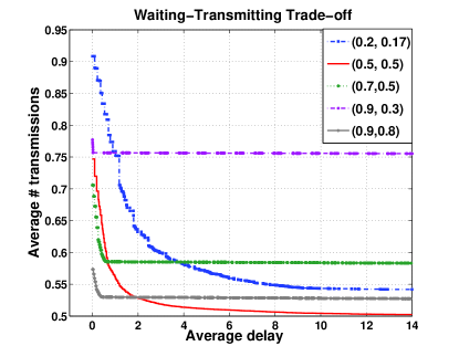
Figure 4: Trade-off between average delay and number of transmissions in a single relay using queue-length based threshold (QLT) policy for different Bernoulli arrival rates $(p_{1},p_{2})$.

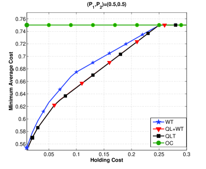
Figure 5: Comparison of the minimum average cost (per packet) in a single relay with Bernoulli arrival rates $(0.5,0.5)$, for different policies, where the costs are normalized by the transmission cost.

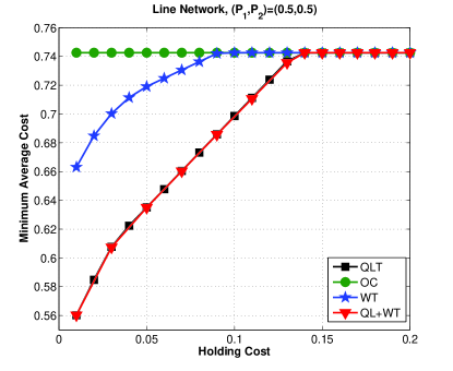
Figure 6: Comparison of different policies in a line network with two intermediate nodes and two Bernoulli flows with mean arrival rates $(0.5,0.5)$.

VIII Extensions

We have seen that the average-optimal policy is stationary and threshold based for the i.i.d. arrival process with the service rate of 1 packet per time slot. Two more general models are discussed here. We focus on the character of the optimality equation which results in the structure of the average-optimal policy.

VIII-A Batched service

Assume that the relay $R$ can serve a group of packets with the size of $\mathcal{M}$ at end of the time slot. At the end of every time slot, relay $R$ decides to transmit, $a_{t}=1$, or to wait $a_{t}=0$. The holding cost per unit time for a packet is $C_{H}$, while $C_{T}$ is the cost to transmit a batched packet. Then the immediate cost is

$$C^{(\mathcal{M})}(Q_{t},a_{t})$$

$$= C_{H}([Q^{(1)}_{t}-a_{t}\mathcal{M}]^{+}+[Q^{(2)}_{t}-a_{t}\mathcal{M}]^{+})+C_{T}a_{t}.$$

We also want to find the optimal policy $\theta^{*}$ that minimizes the long-time average cost $V^{(\mathcal{M})}(\theta)$, called $\mathcal{M}$-MDP$\{(Q_{t},a_{t}),t\geq 0\}$ problem,

$$V^{(\mathcal{M})}(\theta)=\lim_{K\rightarrow\infty}\frac{1}{K+1}\mathbb{E}_{\theta}\left[\sum_{t=0}^{K}C^{(\mathcal{M})}(Q_{t},a_{t})|Q_{0}=(0,0)\right].$$

Notice that the best policy might not just transmit when both queues are non-empty. When $\mathcal{M}>1$, $R$ might also want to wait even if $Q^{(1)}_{t}Q^{(2)}_{t}>0$ because the batched service of size less than $\mathcal{M}$ has the same transmission cost $C_{T}$. The optimality equation of the expected $\alpha$-discounted cost is revised as

$$V^{(\mathcal{M})}_{\alpha}(i,j)= \min_{a\in\{0,1\}}\Bigl{[}C_{H}([i-a\mathcal{M}]^{+}+[j-a\mathcal{M}]^{+})+C_{T}a+$$

$$\hskip 5.69046pt\mathbb{E}[V^{(\mathcal{M})}_{\alpha}([i-a\mathcal{M}]^{+}+\mathcal{A}_{1},[j-a\mathcal{M}]^{+}+\mathcal{A}_{2})]\Bigr{]}.$$

We can get the following results.

Theorem 24.

Given $\alpha$ and $\mathcal{M}$, $V^{(\mathcal{M})}_{\alpha}(i,j)$ is non-decreasing, submodular, and $\mathcal{M}$-subconvex. Moreover, there is an $\alpha$-optimal policy that is of threshold type. Fixed $j$, the $\alpha$-optimal policy is monotone w.r.t. $i$, and vice versa.

Theorem 25.

Consider any i.i.d. arrival processes to both queues. For the $\mathcal{M}$-MDP$\{(Q_{t},a_{t}),t\geq 0\}$, the average-optimal policy is of threshold type. Given $j=\tilde{j}$ fixed, there exists the optimal threshold $L^{*}_{\tilde{j}}$ such that the optimal stationary and deterministic policy in state $(i,\tilde{j})$ is to wait if $i\leq L^{*}_{\tilde{j}}$, and to transmit if $i>L^{*}_{\tilde{j}}$. Similar argument holds for the other queue.

VIII-B Markov-Modulated Arrival Process

While the i.i.d. arrival process is examined so far, a specific arrival process with memory is studied here, i.e., Markov-modulated arrival process (MMAP). The service capacity of $R$ is focused on $\mathcal{M}=1$ packet. Let $\mathcal{N}^{(i)}=\{0,1,\cdots,N^{(i)}\}$ be the state space of MMAP at node $i$, with the transition probability $p^{(i)}_{k,l}$ where $k,l\in\mathcal{N}^{(i)}$. Then the number of packets generated by the node $i$ at time $t$ is $\mathcal{N}^{(i)}_{t}\in\mathcal{N}^{(i)}$. Then the decision of $R$ is made based on the observation of $(Q^{(1)}_{t},Q^{(2)}_{t},\mathcal{N}^{(1)}_{t},\mathcal{N}^{(2)}_{t})$. Similarly, the objective is to find the optimal policy that minimizes the long-term average cost, named MMAP-MDP$\{((Q^{(1)}_{t},Q^{(2)}_{t},\mathcal{N}^{(1)}_{t},\mathcal{N}^{(2)}_{t}),a_{t}):t\geq 0\}$ problem. The optimality equation of the expected $\alpha$-discounted cost becomes

$$V^{\text{MMAP}}_{\alpha}(i,j,n_{1},n_{2})$$

$$= \min_{a\in\{0,1\}}[C_{H}([i-a]^{+}+[j-a]^{+})+C_{T}a+$$

$$\hskip 8.5359pt\alpha\sum_{k=0}^{N^{(1)}}\sum_{l=0}^{N^{(2)}}p^{(1)}_{n_{1},k}p^{(2)}_{n_{2},l}V^{\text{MMAP}}_{\alpha}([i-a]^{+}+k,[j-a]^{+}+l,k,l)].$$

Then we can conclude the following results.

Theorem 26.

Given $n_{1}\in\mathcal{N}^{(1)}$ and $n_{2}\in\mathcal{N}^{(2)}$, $V^{\text{MMAP}}_{\alpha}(i,j,n_{1},n_{2})$ is non-decreasing, submodular, and subconvex w.r.t. $i$ and $j$. Moreover, there is an $\alpha$-optimal policy that is of threshold type. Fixed $n_{1}$ and $n_{2}$, the $\alpha$-optimal policy is monotone w.r.t. $i$ when $j$ is fixed, and vice versa.

Theorem 27.

Consider any MMAP arrival process. For the MMAP-MDP$\{((Q^{(1)}_{t},Q^{(2)}_{t},\mathcal{N}^{(1)}_{t},\mathcal{N}^{(2)}_{t}),a_{t}):t\geq 0\}$, the average-optimal policy is of multiple thresholds type. There exists a set of optimal thresholds $\{L^{*}_{1,n_{1},n_{2}}\}$ and $\{L^{*}_{2,n_{1},n_{2}}\}$, where $n_{1}\in\mathcal{N}^{(1)}$ and $n_{2}\in\mathcal{N}^{(2)}$, so that the optimal stationary decision in states $(i,0,n_{1},n_{2})$ is to wait if $i\leq L^{*}_{1,n_{1},n_{2}}$, and to transmit without coding if $i>L^{*}_{1,n_{1},n_{2}}$; while in state $(0,j,n_{1},n_{2})$ is to wait if $j\leq L^{*}_{2,n_{1},n_{2}}$, and to transmit without coding if $j>L^{*}_{2,n_{1},n_{2}}$.

IX Conclusion

In this paper we investigate the delicate trade-off between waiting and transmitting using network coding. We started with the idea of exploring the whole space of history dependent policies, but showed step-by-step how we could move to simpler regimes, finally culminating in a stationary deterministic queue-length threshold based policy. The policy is attractive because its simplicity enables us to characterize the thresholds completely, and we can easily illustrate its performance on multiple networks. We showed by simulation how the performance of the policy is optimal in the Bernoulli arrival scenario, and how it also does well in other situations such as for line networks. Our results also have some bearing on the general problem of queuing networks with shared resources that we will explore in the future.

X Acknowledgement

The authors are grateful to Rajesh Sundaresan, Vivek Borkar, and Daren B. H. Cline for the useful discussions. This material is based upon work partially supported by the AFOSR under contract No. FA9550-13-1-0008.

References

- [1] M. Effros, T. Ho, and S. Kim, “A Tiling Approach to Network Code Design for Wireless Networks,” Proc of IEEE ITW, pp. 62–66, 2006.
- [2] R. Ahlswede, N. Cai, S. Y. R. Li, and R. W. Yeung, “Network Information Flow,” IEEE Trans. Inf. Theory, vol. 46, pp. 1204–1216, 2000.
- [3] S. Katti, H. Rahul, W. Hu, D. Katabi, M. Medard, and J. Crowcroft, “XORs in the Air: Practical Wireless Network Coding,” IEEE/ACM Trans. Netw., vol. 16, pp. 497–510, 2008.
- [4] S. Chachulski, M. Jennings, S. Katti, and D. Katabi, “Trading Structure for Randomness in Wireless Opportunistic Routing,” Proc. of ACM SIGCOMM, pp. 169–180, 2007.
- [5] Y. E. Sagduyu and A. Ephremides, “Cross-Layer Optimization of MAC and Network Coding in Wireless Queueing Tandem Networks,” IEEE Trans. Inf. Theory, vol. 54, pp. 554–571, 2008.
- [6] A. Khreishah, C. C. Wang, and N. Shroff, “Cross-Layer Optimization for Wireless Multihop Networks with Pairwise Intersession Network Coding,” IEEE J. Sel. Areas Commun., vol. 27, pp. 606–621, 2009.
- [7] V. Reddy, S. Shakkottai, A. Sprintson, and N. Gautam, “Multipath Wireless Network Coding: A Population Game Perspective,” Proc of IEEE INFOCOM, 2010.
- [8] A. Eryilmaz, D. S. Lun, and B. T. Swapna, “Control of Multi-Hop Communication Networks for Inter-Session Network Coding,” IEEE Trans. Inf. Theory, vol. 57, pp. 1092–1110, 2011.
- [9] T. Ho and H. Viswanathan, “Dynamic Algorithms for Multicast With Intra-Session Network Coding,” IEEE Trans. Inf. Theory, vol. 55, pp. 797–815, 2009.
- [10] Y. Xi and E. M. Yeh, “Distributed Algorithms for Minimum Cost Multicast With Network Coding,” IEEE/ACM Trans. Netw., vol. 18, pp. 379–392, 2010.
- [11] E. C. Ciftcioglu, Y. E. Sagduyu, R. A. Berry, and A. Yener, “Cost-Delay Tradeoffs for Two-Way Relay Networks,” IEEE Trans. Wireless Commun., pp. 4100–4109, 2011.
- [12] M. L. Puterman, Markov Decision Processes: Discrete Stochastic Dynamic Programming. The MIT Press, 1994.
- [13] S. M. Ross, Introduction to Stochastic Dynamic Programming. Academic Press, 1994.
- [14] L. I. Sennott, Stochastic Dynamic Programming and the Control of Queueing Systems. Wiley-Interscience, 1998.
- [15] D. P. Bertsekas, Dynamic Programming: Deterministic and Stochastic Models. Prentice-Hall, 1987.
- [16] V. S. Borkar, “Control of Markov Chains with Long-Run Average Cost Criterion: The Dynamic Programming Equations,” SIAM Journal on Control and Optimization, pp. 642–657, 1989.
- [17] R. Cavazos-Cadena and L. I. Sennott, “Comparing Recent Assumptions for the Existence of Average Optimal Stationary Policies,” Operations Research Letters, pp. 33–37, 1992.
- [18] M. Schal, “Average Optimality in Dynamic Programming with General State Space,” Mathematics of Operations Research, pp. 163–172, 1993.
- [19] L. I. Sennott, “Average Cost Optimal Stationary Policies in Infinite State Markov Decision Processes with Unbounded Costs,” Operations Research, vol. 37, pp. 626–633, 1989.
- [20] G. Koole, Monotonicity in Markov Reward and Decision Chains: Theory and Applications. Now Publishers Inc, 2007.
- [21] S. R. Kulkarni and P. Viswanath, “A deterministic approach to throughput scaling in wireless networks,” IEEE Transactions on Information Theory, vol. 50, no. 6, pp. 1041–1049, 2004.
- [22] S. Shakkottai, X. Liu, and R. Srikant, “The multicast capacity of large multihop wireless networks,” IEEE/ACM Transactions on Networking, vol. 18, no. 6, pp. 1691–1700, 2010.
- [23] V. S. Borkar, “Convex analytic methods in markov decision processes,” in Handbook of Markov Decision Processes, E. Feinberg and A. Shwartz, Eds. Springer US, 2002, pp. 347–375.
- [24] S. Meyn, Control Techniques for Complex Networks. Cambridge University Press, 2007.