The effects of betatron motion on the preservation of FEL microbunching
Abstract
In some options for circular polarization control at X-ray FELs, a helical radiator is placed a few ten meters distance behind the baseline undulator. If the microbunch structure induced in the baseline (planar) undulator can be preserved, intense coherent radiation is emitted in the helical radiator. The effects of betatron motion on the preservation of micro bunching in such in-line schemes should be accounting for. In this paper we present a comprehensive study of these effects. It is shown that one can work out an analytical expression for the debunching of an electron beam moving in a FODO lattice, strictly valid in the asymptote for a FODO cell much shorter than the betatron function. Further on, numerical studies can be used to demonstrate that the validity of such analytical expression goes beyond the above-mentioned asymptote, and can be used in much more a general context. Finally, a comparison with Genesis simulations is given.
DEUTSCHES ELEKTRONEN-SYNCHROTRON
Ein Forschungszentrum der Helmholtz-Gemeinschaft
DESY 11-081
May 2011
The effects of betatron motion on the preservation of FEL microbunching
Gianluca Geloni,
European XFEL GmbH, Hamburg
Vitali Kocharyan and Evgeni Saldin
Deutsches Elektronen-Synchrotron DESY, Hamburg ISSN 0418-9833 NOTKESTRASSE 85 - 22607 HAMBURG
1 Introduction
The LCLS baseline includes a planar undulator system, which produces intense linearly polarized light in the wavelength range between nm and nm LCLS2 . Several schemes using helical undulators have been proposed for polarization control at the LCLS setup GENG , KUSK , OURC . The option presented in OURC , exploits the microbunching of the planar undulator. After the baseline undulator, the electron beam is transported along a m long straight line by FODO focusing system and subsequently passed through a helical radiator. If the microbunch structure of the bunch can be preserved, intense coherent radiation is emitted in the helical radiator. The driving idea of this proposal is that the background linearly-polarized radiation from the baseline undulator is suppressed by spatial filtering. This operation consists in letting radiation and electron beam through horizontal and vertical slits upstream of the helical radiator, where the radiation spot size is about ten times larger than the electron bunch transverse size. The effect of betatron motion on the preservation of micro bunching in such scheme should be accounting for. In fact, the finite angular divergence of the electron beam, linked with the betatron function, yields a spread of the longitudinal velocity leading to microbunching suppression. In OURC we estimated this factor, and concluded that the betatron motion should not constitute a serious problem in proposed scheme.
In this paper we present a comprehensive study of the effect of betatron motion on the microbunch preservation. Our paper is based on the use results of SVEN , where it was showed that in the limit for a small length of a FODO cell with respect to the betatron function value, the longitudinal velocity of an electron, averaged over a FODO cell, is constant through the focusing system. Based on this non-trivial statement, one can work out an analytical expression for the debunching of an electron beam moving in a FODO lattice, strictly valid in the asymptote for a short FODO cell. Further on, numerical studies can be used to demonstrate that the validity of such analytical expression goes beyond the above-mentioned asymptote, and can be used in much more a general context.
The present work is organized as follows. In the following Section 2 we review the main result in SVEN , and we report the expression for the average longitudinal velocity of an electron, which depends on the Courant-Snyder invariant of motion. Based on this result, the analytical expression for the debunching is calculated. In Section 3, the analytical asymptote is cross-checked with numerical calculations, and its validity is extended. A comparison with results obtained with the code Genesis GENE is presented. Finally, in Section 4, we come to conclusions.
2 Analytical study
The starting point for our analysis is a consideration on the longitudinal velocity of an electron in a FODO lattice. As has been shown in SVEN , when the length of the FODO cell is much shorter than the betatron function, the longitudinal velocity of the electron, averaged over one FODO cell length, is constant. From a mathematical viewpoint, this result may be obtained with simple analytical calculations from Eq. (6) and Eq. (7) of reference SVEN . We will begin to consider a 2D motion on the plane. The longitudinal velocity of a certain electron can be written as , where is the electron speed, and is the angle formed at each point of the electron trajectory with the longitudinal axis. When, as is the case for ultrarelativistic electrons moving along the axis, , one can expand the trigonometric function and obtain , where is given by Eq. (6) and Eq. (7) of reference SVEN . When the length of FODO cell, , is much shorter then betatron function, the magnitude of the Twiss parameter approaches unity, and one can re-write these two equations approximatively as:
| (3) | |||
| (4) |
Here is the particle Courant-Snyder invariant, while and are the betatron function and the betatron phase respectively. Averaging over one FODO cell length one obtains:
| (5) |

which is proportional to the Courant-Snyder invariant , and is independent of . This result looks at first glance surprising. In fact, a glance of a typical electron trajectory shows, Fig. 1 shows an overall oscillatory trajectory, and one would expect that the longitudinal velocity at , where the electron trajectory forms an angle with the axis, should be smaller than, for example, that at m, where the trajectory is almost parallel to the axis. The physical explanation is that the longitudinal velocity is decreased at the position for at m, by the presence of sharp oscillations on the scale of the FODO cell, which, as demonstrated above, lead to a constant average longitudinal velocity.
We will now make use of Eq. (5) to study the effects of the betatron motion on the preservation of FEL microbunching. Consider an electron beam carrying an average current . Let us superimpose an initial modulation at a given frequency . The total current can be written as a function of the phase , with the longitudinal position, the time, the longitudinal velocity as
| (6) |
Similarly, given the unmodulated longitudinal particle density , being the electron charge, the longitudinal particle density after the initial modulation is given by
| (7) |
Here describes the initial bunching. The relation between and the bunching factor , which can be often found in literature is given by
| (8) |
where is the total number of particles within a wavelength , i.e. , and is the phase of each particle.
The ratio , with the average betatron function, is the first relevant parameter of our problem. We will assume , so that Eq. (5) can be used for the average longitudinal velocity of an electron. The phase difference of an electron with Courant-Snyder invariant with respect to one moving on-axis, after a given distance can thus be written as . Since the rms value for is the geometrical emittance one obtains, parametrically, is of order , which is the second and last relevant parameter of our problem. No debunching is expected for .
Under the accepted approximation it is possible to derive an analytical expression for the evolution of the bunching factor along the FODO lattice. In fact, the influence of the betatron motion alone can be modelled by substituting the phase of each individual electron with where, as described above,
| (9) |
The bunching factor after the propagation along the FODO cell can therefore be written as an average over the distribution of , which we call , as
| (11) | |||||
Using
| (12) |
remembering Eq. (7) and Eq. (8) one obtains from Eq. (11) the following expression for the ratio between final and initial bunching:
| (13) |
The integral can be calculated analytically yielding the final result
| (14) |


Note that is not a real number. The physical interpretation of is that of the evolution of the amplitude of the bunching. The physical interpretation of is that of the evolution of the phase of the bunching. In other words, the bunching evolves in modulus and phase along the FODO lattice. Also, notice that is independent of the initial definition of the bunching, or . In both cases, the final bunching can be found by multiplying the initial bunching by . Modulus and phase of are plotted in Fig. 2 as a function of the parameter .
Finally, we note that all considerations have been made for a 2D motion on the plane. However, generalizing to a 3D motion is trivial. One needs to account the divergence , giving an extra contribution to the phase formally identical as that for the horizontal direction, once the horizontal beta function is substituted with the vertical one. One obtains that , with formally identical to Eq. (14).
3 Numerical study
In order to study the influence of the betatron beating on the microbunch suppression and to have an idea about the accuracy of our analytical asymptotic results, we simulated the evolution of the bunching numerically. In particular, we considered a periodic lattice composed of drift, focusing element in the thin-lens approximation, drift, defocusing element. For simplicity, we considered the motion in the direction, so that Eq. (14) could be used to compare with debunching calculated numerically. In the numerical calculations, the magnetic structure is defined, in terms of quadrupole strength and length of the drifts. Then, the Twiss parameters at the beginning of the setup are calculated, and used to generate the horizontal phase-space distribution of electrons. Each particle is tracked through the setup in a linear matrix approach, and the trajectory is calculated. Knowing the trajectory for each electron it is then straightforward to calculate the curvilinear distance traveled. Comparison with the length of the setup allows one to recover the phase difference and to calculate .
We began our numerical investigations setting the average betatron function value m, and the length of the cell m. This choice for the length of the FODO cell allows to consider the asymptote nearly satisfied. The debunching module was calculated for different emittance value. A comparison with calculated analytically from Eq. (14) is shown in Fig. 3. The number of particles is varied from to to achieve a good accuracy, and is not constant for the calculated points. For the sake of exemplification, the white circle in Fig. 3 corresponds to particles, whereas the black circle at the same emittance value corresponds to particles. The good agreement between numerical and analytical results was to be expected on the basis of the asymptote .

An interesting result can be achieved by fixing the emittance (in our case m), and changing , keeping the other quantities as in the previous example. This means that still m. In this way one can sweep through different values of the parameter . In particular, we calculated numerically the value of for . The result of the comparison with the asymptotic for in Eq. (14) is shown in Fig. 4. A very good agreement can be seen even for values not much smaller than unity. Since the average beta function is related to the betatron phase and to the length of the FODO cell by , the maximuum value achievable for turns out to be limited to about for a working focusing system. From this numerical analysis it follows that Eq. (14) can be used not only in the asymptotic case for but, with the good accuracy given in Fig. 4, practically in all cases. This is the main result of this work.

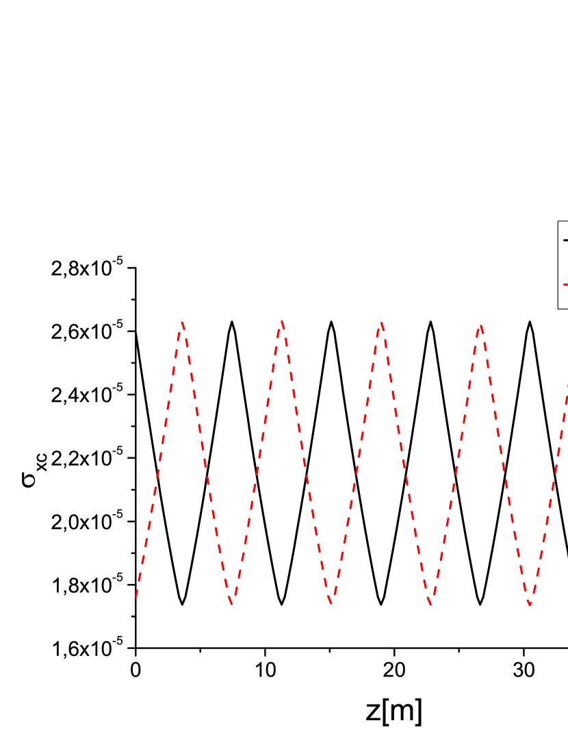
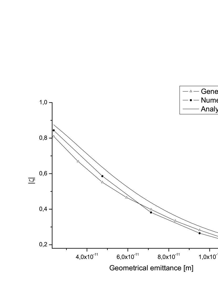
Finally, we present a comparison between obtained from Eq. (14), calculated numerically as above, and derived using the FEL code Genesis GENE . We assumed a cell length of m, so that we set m, and a drift distance equivalent to cells, i.e. m. We set both horizontal and vertical average betatron function to m. In order to simulate the focusing system in Genesis, without the influence of the undulators we set the electron beam current to zero, we switched off the undulator focusing, and we prepared a Genesis particle file with a given density bunching at the modulation wavelength nm, so that it was matched with the FODO beam transport line. The electron beam energy was set to GeV. All particles in the particle file were set with the same energy: as a result effects of the momentum compaction factor were excluded. The beam was propagated through the setup. The evolution of the rms horizontal and vertical size as a function of the distance along the setup is shown in Fig. 5. At the end of the setup, the final particle beam was extracted, allowing for a comparison of the final bunching with respect to the initial bunching. The debunching as a function of the geometrical emittance is presented in Fig. 6.
4 Conclusions
In this paper we derived an analytical expression for the debunching of an modulated electron beam through a FODO focusing structure. The expression is very simple, and can be practically used for any value in the parameter space.
5 Acknowledgements
We are grateful to Massimo Altarelli, Reinhard Brinkmann, Serguei Molodtsov and Edgar Weckert for their support and their interest during the compilation of this work.
References
- [1] P. Emma et al., Nature photonics doi:10.1038/nphoton.2010.176 (2010)
- [2] H.Geng, Y. Ding and Z. Huang, Nucl.Instr. and Meth. A 622 (2010) 276
- [3] B. Kuske and J. Bahrdt, FEL Conference Proceedings 2008 p.348, ”Tolerance studies for APPLE undulators in FEL facilities”
- [4] G. Geloni, V. Kocharyan and E. Saldin, ”Circular polarization control for the LCLS baseline in the soft X-ray regime”, DESY 10-252 (2010).
- [5] S. Reiche, Nucl. Instrum. Methods A, 445, 90 (2000)
- [6] S Reiche et al., Nucl. Instr. and Meth. A 429, 243 (1999).