On exact time-averages of a massive Poisson particle

Abstract

In this work we study, under the Stratonovich definition, the problem of the damped oscillatory massive particle subject to a heterogeneous Poisson noise characterised by a rate of events, $\lambda(t)$, and a magnitude, $\Phi$, following an exponential distribution. We tackle the problem by performing exact time-averages over the noise in a similar way to previous works analysing the problem of the Brownian particle. From this procedure we obtain the long-term equilibrium distributions of position and velocity as well as analytical asymptotic expressions for the injection and dissipation of energy terms. Considerations on the emergence of stochastic resonance in this type of system are also set forth.

Keywords: Stochastic processes, Rigorous results in statistical mechanics

1 Introduction

Stochastic processes have long surpassed the limits of a mere probability theory subject establishing itself as a topic of capital importance in various disciplines which go from molecular motors to internet traffic analysis [1, 2, 3]. In what concerns statistical mechanics, we owe its introduction to the study of Brownian motion by means of the Langevin equation [4]. Explicitly, a random term was added to the classical laws of movement in order to emulate the collisions between the particle under study and the particles of the supporting medium assuming that the jolts between particles cannot be deterministically written down [5, 6]. This approach was promptly adopted in other problems, particularly those coping with systems that exhibit a large number of degrees of freedom. Therehence, the allocation to the noise of the microscopic features and playing interactions of the system has become a common practice. Due to the accurate descriptions of diverse systems, the use of the Wiener process (driftless Brownian motion) [7, 8] has assumed a leading role in widespread fields. However, this corresponds to a very specific sub-class in the wider Lévy class of stochastic process [9]. Specifically, the Wiener process corresponds to the case of a stochastic process for which the increments are independent, stationary (in the sense that the distribution of any increment depends only on the time interval between events) associated with a Gaussian distribution thus having all statistical moments finite. Moreover, its intimate relation to the Fokker-Planck Equation has put the Wiener process and its adaptive processes in the limelight.

Despite the ubiquity of the Wiener process, several other processes, either in Nature or man made, are quite distinct [10, 11, 12]. Particularly, they can be associated with (compound) Poisson processes in which the independent increments befall upon a rate $\lambda\left(t\right)$ with its magnitude related to a certain probability density function. For this kind of noise, it was previously shown that the traditional Fokker-Planck approach cannot be applied because the Kramers-Moyal moments from the third order on do not vanish [13]. Consequently, the equation for the evolution of the probability density function cannot be exactly written as a second-order differential equation, but it maintains its full (infinite) Kramers-Moyal form instead [13]. As it turns out, a complete solution is quite demanding for most of the cases.

In this manuscript we study a damped harmonic oscillator subjected to a random force described by a heterogeneous compound Poisson process which can be replicated by means of a RLC circuit with random injections of power, or several other dynamical processes at the so-called complex system level. Moreover, such kind of problems often conduce to the emergence of stochastic resonance [14, 15] that is found in so diverse problems spanning from neuroscience and Parkinson’s disease [16] to micromechano-electronics [17]. Although this specific system (and its variants) has been studied by different authors [1], in this manuscript we survey the problem assuming a very fundamental and different approach. Explicitly, we make direct averages over the noise for different quantities of interest, in the reciprocal space-time (Fourier-Laplace) domain, by a method that can be applied to the treatment of coloured noise [18], multiple types of noise [19], thermal conductance problems [20], or work fluctuation theorems for small mechanical models [21]. Namely, within the Stratonovich definition, we first focus our efforts on the evaluation of the steady state probability density function (PDF). Afterwards, we study the evolution of the injected (dissipated) power into (out of) the system as well as the total energy of the system and the emergence of stochastic resonance.

2
Exactly solvable model

Our system can be described by two coupled stochastic differential equations:

$$\dot{x}(t)=v(t),$$ (1)

$$M\,\dot{v}(t)=-k_{0}x(t)-\gamma v(t)+\eta(t),$$ (2)

where $\eta$ is a compound heterogeneous Poisson noise,

$$\eta\left(t\right)=\sum\nolimits_{\ell}\Phi\left(t\right)\,\delta\left(t-t_{\ell}\right),$$ (3)

for which the shots (events) occur at a rate $\lambda\left(t\right)$. Specifically, we will study the following time dependency,

$$\lambda(t)=\lambda_{0}\left[1+A\cos(\omega\,t)\right],\qquad\left(0\leq A<1\right).$$ (4)

The case $A=0$ yields the standard homogeneous case. We have opted for a sinusoidal dependence of the rate $\lambda\left(t\right)$ because of its ubiquity in a wide range of phenomena [22].

The Poisson process, $\mathbb{P}$, is a continuous-time stochastic process belonging to the class of independently distributed random variables whose generating function between $t$ and $t+\Delta t$ is

$$\mathcal{G}_{t,t+\Delta t}\left(z\right)=\exp\left[\left(z-1\right)\int_{t}^{t+\Delta t}\lambda\left(t^{\prime}\right)\,dt^{\prime}\right],$$ (5)

which is defined by the rate of events, $\lambda\left(t\right)$, such that,

$$\left\langle n\left(t\right)\right\rangle=\int_{0}^{t}\lambda\left(t^{\prime}\right)\,dt^{\prime},$$ (6)

(we use the notation $\left\langle\left(\ldots\right)\right\rangle$ to represent averages over samples whereas $\overline{\left(\ldots\right)}$ symbolise averages over time). According to its definition, it is only possible to have a single event at instant $t$. Therefore, from Eq. (5) and considering the limit $\Delta t\rightarrow 0$, one can compute the probability that an event occurs is given by $\int_{t}^{t+\Delta t}\lambda\left(t\right)\,dt$, while $1-\int_{t}^{t+\Delta t}\lambda\left(t\right)\,dt$ is the probability of zero events. Again, from Eq. (5), we can analyse the probability distribution of the inter-arrival time PDF, $\mathcal{T}\left(\tau\right)$. The probability that having an event at time $t$ the next event occurs at $t+\tau$ is given by,

$$p\left(\tau|t\right)=\frac{d}{d\tau}\left(1-\exp\left[-\int_{t}^{t+\tau}\lambda\left(t^{\prime}\right)\,dt^{\prime}\right]\right).$$ (7)

For a heterogeneous Poisson process, one must still pay attention that each instant has a different weight in the calculation, exactly because of the time dependence of $\lambda$. This weight, $f\left(t\right)$, is defined by

$$f\left(t\right)=\lambda\left(t\right)/\int_{0}^{T}\lambda\left(t^{\prime}\right)\,dt^{\prime},$$ (8)

for a heterogeneous Poisson process taking place in the time interval from $0$ to $T$. Thence, combining Eqs. (7) and (8) and integrating over time one obtains,

$$\mathcal{T}\left(\tau\right)=\int_{0}^{T-\tau}f\left(t\right)\,p\left(\tau|t\right)\,dt.$$ (9)

Concerning the amplitude, $\Phi$, despite being possible to consider several distribution functions, we will restrict our study to the classical exponential probability density function for white shot-noises,

$$P\left(\Phi\right)=\bar{\Phi}^{-1}\exp\left[-\frac{\Phi}{\bar{\Phi}}\right],$$

whose $n$-th order raw moment is, $\overline{\Phi^{n}}=n!\,\bar{\Phi}^{n}$.

Going back to Eq. (3), we can define the Poisson patch, $I$, between $t$ and $t+\tau,$

$$I\left(\tau\right)\equiv\mathbb{P}\left(t+\tau\right)-\mathbb{P}\left(t\right)=\int_{t}^{t+\tau}d\mathbb{P}=\int_{t}^{t+\tau}\eta\left(t^{\prime}\right)\,dt^{\prime},$$

from which we can set out,

$$\int dI\left(\tau^{\prime}\right)=\int d\mathbb{P}=\int\eta\left(t^{\prime}\right)\,\,dt^{\prime},$$

where we have omitted the time dependence of the patch for the sake of simplicity. The average of the Poisson patch is,

$$\left\langle I\left(\tau\right)\right\rangle_{c}=\left\langle I\left(\tau\right)\right\rangle=\bar{\Phi}\int_{t}^{t+\tau}\lambda\left(t^{\prime}\right)\,dt^{\prime}.$$

and its covariance,

$$I\left(\tau_{1}\right)I\left(\tau_{2}\right)=\int_{t}^{t+\tau_{1}}\eta\left(t^{\prime}\right)\,dt^{\prime}\int_{t}^{t+\tau_{2}}\eta\left(t^{\prime\prime}\right)\,dt^{\prime\prime}.$$

which yields after averaging,

$$\left\langle I\left(\tau_{1}\right)\,I\left(\tau_{2}\right)\right\rangle_{c} = \overline{\Phi^{2}}\int_{t}^{t+\tau_{1}}\int_{t}^{t+\tau_{2}}\lambda\left(t^{\prime\prime}\right)\,\delta\left(t^{\prime\prime}-t^{\prime}\right)\,dt^{\prime\prime}\,dt^{\prime}$$

$$= \overline{\Phi^{2}}\int_{t}^{t+\min\left(\tau_{2},\tau_{1}\right)}\lambda\left(t^{\prime}\right)\,\,dt^{\prime}.$$

These moments can be straightforwardly generalised to,

$$I\left(t\right)^{n}=\int_{t}^{t+\tau}dt_{1}\ldots\int_{t}^{t+\tau}dt_{n}\,\eta(t_{1})\ldots\eta(t_{n}).$$

The noise cumulant averages are,

$$\langle I\left(t\right)^{n}\rangle_{c}=\int_{t}^{t+\Delta t}dt_{1}\ldots\int_{t}^{t+\Delta t}dt_{n}\,\langle\eta(t_{1})\ldots\eta(t_{n})\rangle_{c}=\lambda\left(t\right)\,\overline{\Phi^{n}}\,\Delta t.$$

This implies that the noise cumulant correlations are identified as [13],

$$\langle\eta(t_{1})\ldots\eta(t_{n})\rangle_{c}=\lambda(t_{1})\,\overline{\Phi^{n}}\,\delta(t_{1}-t_{2})\ldots\delta(t_{n-1}-t_{n}).$$ (10)

Accordingly,

$$\int_{t}^{t+\Delta t}\prod_{i=1}^{n}dt_{i}\,\langle\eta(t_{1})\ldots\eta(t_{n})\rangle_{c} = \int_{t}^{t+\Delta t}\prod_{i=1}^{n}dt_{i}\,\lambda_{0}\left(1+A\cos(\omega\,t_{1})\right)\Phi^{n}\prod_{j=1}^{n-1}\delta(t_{j}-t_{j+1})$$ (11)

$$= \lambda_{0}\,\overline{\Phi^{n}}\int_{t}^{t+\Delta t}dt_{1}\left(1+A\cos(\omega\,t_{1})\right)$$

$$= \lambda_{0}\,\overline{\Phi^{n}}\left[\Delta t+2\frac{A}{\omega}\sin\left(\omega\,\frac{\,\Delta\,t}{2}\right)\,\cos(\omega\,t)\right].$$

Taking into account the limit, $\Delta t\rightarrow 0$, the previous expression tends to $\lambda_{0}\,\overline{\Phi^{n}}\,\Delta t\left(1+A\cos(\omega\,t)\right)$ and thus,

$$\int_{t}^{t+\Delta t}dt_{1}\ldots\int_{t}^{t+\Delta t}dt_{n}\,\langle\eta(t_{1})\ldots\eta(t_{n})\rangle_{c}=\lambda_{0}\,\overline{\Phi^{n}}\left[1+A\cos\left(\omega t\right)\right]\,\Delta t=\lambda\left(t\right)\,\overline{\Phi^{n}}\,\Delta t.$$ (12)

In the case $n=1$, Eq. (12) satisfies the relation $\langle I\left(t\right)\rangle=\lambda\left(t\right)\,\bar{\Phi}\,\Delta t$, as expected.

Throughout this manuscript we employ the Stratonovich representation for the noise,

$$\left\langle\int_{t}^{t+\Delta t}I\,dI\right\rangle_{c}=\left\langle\int_{t}^{t+\Delta t}\frac{dI^{2}}{2}\right\rangle_{c}=\lambda\left(t\right)\,\overline{\Phi^{2}}\,\frac{\Delta t}{2},$$

where the effective noise in a interval $dt$ is computed as the average of the noise at $t$ and $t+dt$.

2.1 Laplace transformations

Taking the Laplace transformations of Eqs. (1) and (2) (with Re$(s)>0$) we obtain,

$$s\,\tilde{x}(s)=\tilde{v}(s).$$ (13)

Defining,

$$R(s)\,\equiv\,s^{2}+\frac{\gamma}{M}s+\frac{k_{0}}{M}=(s-\kappa_{+})(s-\kappa_{-}),$$ (14)

we can write,

$$\tilde{x}(s)=\frac{\tilde{\eta}(s)}{M\,R(s)},$$ (15)

the singularities of which (the zeroes of $R(s)$) are located at,

$$\kappa_{\pm}=-\theta\pm\,i\,\Omega.$$ (16)

with $\theta=\frac{\gamma}{2\,M}$, $\omega_{0}^{2}=\frac{k_{0}}{M}$ and $\Omega=\sqrt{\omega_{0}^{2}-\theta^{2}}.$

For the Poisson process with time-dependent rate, Eq. (4), the Laplace transform of the noise averages yields,

$$\langle\tilde{\eta}(z_{1})\ldots\tilde{\eta}(z_{n})\rangle_{c} = \int_{0}^{\infty}\prod_{i=1}^{n}dt_{i}\,\exp\left\{-\sum_{l=1}^{n}z_{l}t_{l}\right\}\langle\eta(t_{1})\ldots\eta(t_{n})\rangle_{c}$$ (17)

$$= \lambda_{0}\,\overline{\Phi^{n}}\int_{0}^{\infty}\prod_{i=1}^{n}dt_{i}\,\delta(t_{1}-t_{2})\ldots\delta(t_{n-1}-t_{n})$$

$$\times\left[1+A\cos(\omega\,t_{1})\right]\exp\left\{-\sum_{l=1}^{n}z_{l}t_{l}\right\},$$

for which we can separate out its homogeneous and heterogeneous parts. For the former, we obtain,

$$\mathcal{I}_{1} = \lambda_{0}\,\overline{\Phi^{n}}\int_{0}^{\infty}dt_{1}\,\exp\left\{-t_{1}\sum_{l=1}^{n}z_{l}\right\}$$ (18)

$$= \frac{\lambda_{0}\,\overline{\Phi^{n}}}{\sum_{l=1}^{n}z_{l}},$$

whereas the latter is given by,

$$\mathcal{I}_{2} = \lambda_{0}\,\overline{\Phi^{n}}\,A\int_{0}^{\infty}dt_{1}\,\cos(\omega\,t_{1})\exp\left\{-t_{1}\sum_{l=1}^{n}z_{l}\right\}$$ (19)

$$= \lambda_{0}\,\overline{\Phi^{n}}\frac{A}{2}\left(\frac{1}{\sum_{l=1}^{n}z_{l}-\mathrm{i}\,\omega}+\frac{1}{\sum_{l=1}^{n}z_{l}+\mathrm{i}\,\omega}\right).$$

The Laplace transform for the noise cumulants is thus given by:

$$\left\langle\tilde{\eta}(z_{1})\ldots\tilde{\eta}(z_{n})\right\rangle_{c}=\mathcal{I}_{1}+\mathcal{I}_{2}.$$ (20)

3
Averaged steady state

Instead of equilibrium conditions, a periodically forced system reaches a periodically driven state that is characterised by periodic variations of the averages and cumulants of its variables [23]. This behaviour can now be explicitly obtained by the method previously mentioned [18], that we shall use to study the Poisson process. However, taking the time average for the distribution function does make sense given that important quantities, such as the injected and dissipated energies, are well understood when represented by their time averaged values. In the following, we develop the techniques needed for the exact solution of Eqs. (1) and (2) at long times. Our results are comparable with those obtained from the analysis of a single (and sufficiently long) run of the process in which all the values of the observable are treated as equally distributed.

We average the probability distribution over time to obtain the cumulant expansion [1, 18, 19]

$$p_{ss}(x,v) = \sum_{n,m=0}^{\infty}\int_{-\infty}^{+\infty}\frac{dQ}{2\pi}\,\frac{dP}{2\pi}\,e^{\mathrm{i\,}\left(Q\,x+P\,v\right)}\frac{(-\mathrm{i\,}Q)^{n}}{n!}\frac{(-\mathrm{i\,}P)^{m}}{m!}\,\overline{\left\langle x^{n}v^{m}\right\rangle}$$

$$= \int_{-\infty}^{+\infty}\frac{dQ}{2\pi}\,\frac{dP}{2\pi}\,e^{\mathrm{\ i\,}\left(Q\,x+P\,v\right)}\,\exp\left\{\sum_{n,m=0:(m+n>0)}^{\infty\,}\frac{(-\mathrm{i\,}Q)^{n}}{n!}\frac{(-\mathrm{i\,}P)^{m}}{m!}\overline{\left\langle x^{n}v^{m}\right\rangle_{c}}\right\}.$$

Let us work out the exact form of the cumulants in terms of the Laplace transforms of the noise. Applying our definition for computing averages we have,

$$\overline{\left\langle x^{n}v^{m}\right\rangle_{c}} = \lim_{z\rightarrow 0}z\int_{0}^{\infty}dt\,e^{-zt}\,\,\langle x^{n}(t)\,v^{m}(t)\rangle_{c}\,$$

$$= \lim_{z\rightarrow 0}\lim_{\epsilon\rightarrow 0}\int_{-\infty}^{+\infty}\prod_{h=1}^{n}\frac{dq_{h}}{2\pi}\int_{-\infty}^{+\infty}\prod_{j=1}^{m}\frac{dp_{j}}{2\pi}\frac{z}{z-\left[\sum_{h=1}^{n}(\mathrm{i\,}q_{h}+\epsilon)+\sum_{j=1}^{m}(\mathrm{i\,}p_{j}+\epsilon)\right]}$$

$$\times\prod_{h=1}^{n}\frac{1}{\left[M\,R(\mathrm{i\,}q_{h}+\epsilon)\right]}\,\prod_{j=1}^{m}\frac{(\mathrm{i\,}p_{j}+\epsilon)}{\left[M\,R(\mathrm{i\,}p_{j}+\epsilon)\right]}\left\langle\prod_{h=1}^{n}\tilde{\eta}(\mathrm{i\,}q_{h}+\epsilon)\prod_{j=1}^{m}\tilde{\eta}(\mathrm{i\,}p_{j}+\epsilon)\right\rangle_{c},$$

where the integration path for the variables in complex space is the same as in Refs. [18, 19].

4 General steady state distribution

Following the previous section, the Poisson steady state distribution exactly yields,

$$p_{ss}(x,v)=\int_{-\infty}^{+\infty}\frac{dQ}{2\pi}\frac{dP}{2\pi}e^{iQx+iPv}\exp\left\{\sum_{n+m=0:(n+m>0)}^{\infty}\frac{(-\mathrm{i\,}Q)^{n}}{n!}\frac{(-\mathrm{i\,}P)^{m}}{m!}\,\mathcal{P}_{n,m}\right\}.$$ (21)

We may then split Eq. (21) into two parts: term $\mathcal{P}^{\left(1\right)}$ which arises from the time-independent contribution,

$$\mathcal{P}_{n,m}^{\left(1\right)}=\int_{-\infty}^{+\infty}\prod_{h=1}^{m+n-1}\frac{dp_{h}}{2\pi}\frac{\prod_{h=1}^{m}(\mathrm{i\,}p_{h}+\epsilon)}{\prod_{h=1}^{m+n-1}R(\mathrm{i\,}p_{h}+\epsilon)}\,\,\frac{1}{R\left(-\sum_{h=1}^{m+n-1}(\mathrm{i}\,p_{h}+\epsilon)\right)},$$ (22)

and the remaining terms arising from the periodic forcing term,

$$\mathcal{P}_{n,m}^{\left(\pm\right)}=\lim_{z\rightarrow 0}\frac{\lambda_{0}\,A}{2}\int_{-\infty}^{+\infty}\prod_{h=1}^{n+m-1}\frac{dp_{h}}{2\pi}\frac{z}{z\pm\mathrm{i}\,\omega}\frac{\prod_{h=1}^{m}(\mathrm{i\,}p_{h}+\epsilon)}{\prod_{h=1}^{n+m-1}R(\mathrm{i\,}p_{h}+\epsilon)}\frac{1}{R\left(\pm\mathrm{i}\,\omega-\sum_{h=1}^{n+m}(\mathrm{i\,}p_{h}+\epsilon)\right)}.$$

Unrolling Eq. (22), we can determine the different contributions that are allowed to emerge by taking into consideration the different powers of $x$ and $v$ in the cumulant. Accordingly, term $\Psi_{1}$ represents cumulants of zeroth order in the velocity, $\left\langle x^{n}\right\rangle_{c}$,

$$\Psi_{1x}=\sum\limits_{j=0}^{n-1}\left(\begin{array}[]{c}n-1\\ j\end{array}\right)\frac{\left(-1\right)^{n-j-1}}{\left[1,-1\right]^{n-1}\left[j\,,\left(n-j\right)\,\right]\left[\left(j+1\right),\left(n-j-1\right)\,\right]},$$ (23)

and in the position, $\left\langle v^{m}\right\rangle_{c}$,

$$\Psi_{1v}=\sum\limits_{j=0}^{m-1}\left(\begin{array}[]{c}m-1\\ j\end{array}\right)\frac{\mathrm{i}^{\,m}\left(-1\right)^{m-j}\,k_{+}^{\,j}\,k_{-}^{m-j-1}\left[j\,,\left(m-j-1\right)\,\right]}{\left[1,-1\right]^{m-1}\left[j\,,\left(m-j\right)\,\right]\left[\left(j+1\right),\left(m-j-1\right)\,\right]},$$ (24)

Term $\Psi_{2}$ describes cumulants which are such as $\left\langle x^{n-1}v\right\rangle_{c}$,

$$\Psi_{2}=\sum\limits_{j=0}^{n-2}\left(\begin{array}[]{c}n-2\\ j\end{array}\right)\frac{\mathrm{i\,}\left(-1\right)^{n-j-1}}{\left[1,-1\right]^{n-2}}\frac{\left[j,\left(n-j-2\right)\right]}{\left[j,\left(n-j-1\right)\,\right]\left[\left(j+1\right)\,,\left(n-j-2\right)\right]},$$ (25)

and last term $\Psi$₃ represents the remaining combinations of powers of $x^{l}$ and $v^{m}$ with $l+m=n$ and $l\geq 2$,

$$\Psi_{3}\left(m\right) = \sum\limits_{j=0}^{m}\sum_{l=0}^{n-m-1}\left(\begin{array}[]{c}m\\ j\end{array}\right)\left(\begin{array}[]{c}n-m-1\\ l\end{array}\right)\frac{\left(-1\right)^{n-m+j}}{\left[1,-1\right]^{n-m-1}}\frac{\mathrm{i}^{m+1}\,k_{+}^{j}\,k_{-}^{m-j}\,\left[j\,,\left(m-j\right)\,\right]}{\left[1,-1\right]^{m}}\times$$ (30)

$$\times \frac{1}{\left[\left(j+l+1\right)\,,\left(n-m-j-l-1\right)\,\right]\left[\left(j+l\right)\,,\left(n-m-j-l\right)\,\right]},$$ (31)

in which we have the used the following curtailed notation,

$$\left(a\,\kappa_{+}+b\,\kappa_{-}\right)\equiv\left[a,b\right].$$

Therefore, bearing in mind the last definition of the cumulant part of the probability distribution, Eq. (22), we can write it as:

$$p_{ss}(x,v) = \mathcal{F}_{x,v}\left[\exp\left\{\sum_{n,m=0:(m+n>0)}^{\infty}\lambda_{0}\,(n+m)!\,\frac{Q^{n}}{n!}\frac{P^{m}}{m!}\,\left(\mathrm{i\,}\bar{\Phi}\right)^{n+m}\times\right.\right.$$ (32)

$$\left.\left.\left(\Psi_{1x}\,\delta_{m,0}+\Psi_{1v}\,\delta_{n,0}+\Psi_{2}\,\delta_{m,1}+\sum\limits_{m=2}^{n+m-1}\Psi_{3}\left(m\right)\right)\right\}\right],$$

where $\mathcal{F}_{\left(x,v\right)}\left[f\left(Q,P\right)\right]$ represents the 2-dimensional Fourier Transform into position-velocity real space, $\left(x,v\right)$.

Owing to the factor $z/\left(z\mp\mathrm{i}\,\omega\right)$ in terms $\mathcal{P}^{\left(\pm\right)}$ we are able to verify that after performing integrations following the appropriate contour, the $z$ terms hold on up to the end, so that when we finally compute the limit of $z\rightarrow 0$ both contributions vanish. Therefore, for this type of heterogeneity, the steady state distribution bears out the same result as the homogeneous Poisson process with constant rate $\lambda_{0}$. This is quite understandable since we are making a long time average in which the contribution of the periods whose rate is larger than $\lambda_{0}$ kills off the contribution arising from the periods in which the rate is smaller than $\lambda_{0}$ because of the symmetry of the rate around $\lambda_{0}$.

Regarding the marginal steady state distributions,

$$p_{ss}\left(x\right)=\int p_{ss}(x,v)\,dv,$$ (33)

and

$$p_{ss}\left(v\right)=\int p_{ss}(x,v)\,dx,$$ (34)

we start with the probability distribution of the position and following our procedure we obtain,

$$p_{ss}\left(x\right)=\mathcal{F}_{x}\left[\exp\left\{\sum_{n>0}^{\infty}\lambda_{0}\mathrm{\,}Q^{n}\,\bar{\Phi}^{n}\,\Psi_{1x}\right\}\right],$$ (35)

whence we can identify the cumulants,

$$\kappa_{n}\equiv\overline{\left\langle x^{n}\right\rangle_{c}}=n!\lambda_{0}\,\left(\mathrm{i\,}\bar{\Phi}\right)^{n}\,\Psi_{1x}.$$ (36)

Using the property of Pascal triangles,

$$\left(\begin{array}[]{c}n\\ j\end{array}\right)=\left(\begin{array}[]{c}n-1\\ j-1\end{array}\right)+\left(\begin{array}[]{c}n-1\\ j\end{array}\right),$$ (37)

we can write the sum in Eq. (23) over the index $j$ as,

$$\sum_{j=0}^{n-1}\left[\ldots\right]=\,n!\,\left[1,-1\right]^{n-1}\frac{1}{D_{n}},$$ (38)

where,

$$D_{n}=\prod_{j=0}^{n}\left[j,n-j\right].$$ (39)

Accordingly, the cumulants of $p_{ss}(x)$ are

$$\kappa_{n}^{\left(x\right)}=\lambda_{0}\,\,\left(\frac{\bar{\Phi}}{M}\right)^{n}(-1)^{n-1}\frac{\left(n!\right)^{2}}{D_{n}}\qquad\left(n\geq 1\right).$$ (40)

Allowing for Eq. (40), we explicit the average,

$$\overline{\left\langle x\right\rangle}=\bar{\Phi}\,\frac{\lambda_{0}}{k_{0}},$$

and the second-order moment,

$$\overline{\left\langle x^{2}\right\rangle}-\overline{\left\langle x\right\rangle}^{2}=\bar{\Phi}^{2}\frac{\lambda_{0}}{\gamma\,k_{0}}.$$

We have implemented a computational procedure to numerically compute the probability density function of the position at the steady state. Our exhibited numerical results were obtained for different values of $M$, $k_{0}$ and $\gamma$ and fixed values of $\lambda_{0}=10$, $\bar{\Phi}=1$ and $\omega=\pi$ following the implementation described in A. From cases A and B (see values in the figure caption), we can understand that the mass does not impact in both the average and standard deviation and that B and C tally, although each is based on a homogeneous and a heterogeneous process, respectively. Comparing cases A, B and C we verify that the lighter the particle, the skewer the distribution $p_{ss}\left(x\right)$. The results of cases B, C and E help us show that $\gamma$ does not affect the average and finally case F sketches the influence of $k_{0}$. Case D permit us to follow the dependence on the mass. Lighter particles have a skewer distribution. The results are clearly different if we consider a symmetric noise with $\bar{\Phi}=0$. As we will see in the next section, the positive total injection of power associated with this case is replaced by a zero average injection of power related to the steady state average position being zero.

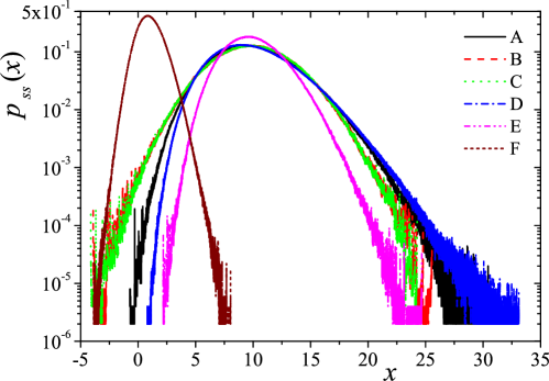
Figure 1: Numerically obtained probability density function $p_{ss}\left(x\right)$ vs position $x$ for various cases with $\lambda_{0}=10$, $\bar{\Phi}=1$ and the noise defined by Eq. (4) with $\omega=\pi$. Following the legend in the figure we have the respective cases, A: $M=1,k_{0}=1,\gamma=1,A=0$, B: $M=10,k_{0}=1,\gamma=1,A=0$, C: $M=10,k_{0}=1,\gamma=1,A=1/2$, D: $M=0.1,k_{0}=1,\gamma=1,A=0$, E: $M=1,k_{0}=1,\gamma=2,A=0$ and F: $M=1,k_{0}=10,\gamma=1,A=0$.

The picture is very much the same for the marginal distribution of the velocity. Namely, from Eq. (34) we get,

$$p_{ss}\left(v\right)=\mathcal{F}_{v}\left[\exp\left\{\sum_{m>0}^{\infty}\lambda_{0}\,P^{m}\,\bar{\Phi}^{m}\,\Psi_{1v}\right\}\right],$$

and consequently the cumulants are,

$$\kappa_{m}^{\left(v\right)}\equiv\overline{\left\langle v^{\,m}\right\rangle_{c}}=m!\,\lambda_{0}\,\left(\mathrm{i\,}\bar{\Phi}\right)^{m}\,\Psi_{1v}.$$ (41)

For the cumulants of the marginal velocity distribution, the calculation turns out much harder and haplessly we have not managed to write it in a compact form as Eq. (35). Nevertheless, we can still write some of them explicitly, such as the first,

$$\kappa_{1}^{v}\equiv\overline{\left\langle v\right\rangle}=0,$$

and the second cumulants,

$$\kappa_{2}^{v}\equiv\overline{\left\langle v^{2}\right\rangle}=\frac{\lambda_{0}\,\bar{\Phi}^{2}}{M\,\gamma}.$$

In Fig. 2, we plot the results of $p_{ss}\left(v\right)$ for the same the numerical implementation of Fig. 1. Once more, we can understand the independence of the probability distribution regarding the amplitude $A$ in Eq. (4). We can also notice the influence of the mass, lighter particles are more sensitive to the noise and thus, for the same noise intensity, they achieve larger positive values of the velocity. Moreover, it is visible that $p_{ss}\left(v\right)$ might be strongly positively skew for light particles. On the other hand, if we consider an average over samples the effect of the amplitude $A$ and frequency $\omega$ of the Poisson noise.

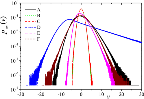
Figure 2: Numerically obtained probability density function $p_{ss}\left(v\right)$ vs scalar velocity $v$ for the same parameters sets of Fig. 1.

5

Injection and dissipation of Energy

An interesting element of study, especially in practical applications such as presented in Ref. [17, 14], concerns the time evolution of energy (related) quantities. This can be checked by heeding the fact that variations of energy in an isolated system equals the total work done by the external forces acting on it, in this case the fluctuating force $\eta$ and the dissipative one $-\gamma v$:

$$\sum W_{F_{ext,i}} = \Delta E_{m}$$ (42)

$$\int\eta\,dx-\gamma\int v\,dx = \frac{1}{2}M\,v\left(t\right)^{2}+\frac{1}{2}k_{0}\,x\left(t\right)^{2}$$

The injection of the energy balance can be also analysed by determining the evolution of the total energy of the particle,

$$\int_{0}^{\tau}\left[\eta\left(t\right)\,v\left(t\right)-\gamma v\left(t\right)^{2}\right]dt=\frac{1}{2}M\,\left.v\left(t\right)^{2}\right|_{t=0}^{t=\tau}+\frac{1}{2}k_{0}\,\left.x\left(t\right)^{2}\right|_{t=0}^{t=\tau}.$$ (43)

In what follows, we shall omit transient terms, keeping the more interesting asymptotic ones whenever possible.

5.1
Energetic considerations

The average values of $\left[v\left(t\right)\right]^{2}$ and $\left[x\left(t\right)\right]^{2}$ that we use in the computation of the total energy can be obtained once more using the Laplace representation,

$$v\left(t\right)^{2} = \int\int v\left(t_{1}\right)v\left(t_{2}\right)\,\delta\left(t-t_{1}\right)\,\delta\left(t-t_{2}\right)\,dt_{1}\,dt_{2}$$

$$= \lim_{\varepsilon\rightarrow 0}\int\int e^{\left(\mathrm{i}\,q_{1}+\mathrm{i}\,q_{2}+2\varepsilon\right)t}\,\tilde{v}\left(\mathrm{i}\,q_{1}+\varepsilon\right)\tilde{v}\left(\mathrm{i}\,q_{2}+\varepsilon\right)\,\frac{dq_{1}}{2\,\pi}\,\frac{dq_{2}}{2\,\pi},$$

whence by averaging and taking into account the second cumulant definition,

$$\left\langle v\left(t\right)^{2}\right\rangle-\left\langle v\left(t\right)\right\rangle^{2} = \lim_{\varepsilon\rightarrow 0}\frac{1}{M^{2}}\int\int e^{\left(\mathrm{i}\,q_{1}+\mathrm{i}\,q_{2}+2\varepsilon\right)t}\,\left(\mathrm{i}\,q_{1}+\varepsilon\right)\left(\mathrm{i}\,q_{2}+\varepsilon\right)\,\times$$

$$\frac{\left\langle\tilde{\eta}\left(\mathrm{i}\,q_{1}+\varepsilon\right)\,\tilde{\eta}\left(\mathrm{i}\,q_{2}+\varepsilon\right)\right\rangle_{c}}{R\left(\mathrm{i}\,q_{1}+\varepsilon\right)\,R\left(\mathrm{i}\,q_{2}+\varepsilon\right)}\frac{dq_{1}}{2\,\pi}\frac{dq_{2}}{2\,\pi},$$

and,

$$\left\langle x\left(t\right)^{2}\right\rangle-\left\langle x\left(t\right)\right\rangle^{2}=\lim_{\varepsilon\rightarrow 0}\frac{1}{M^{2}}\int\int e^{\left(\mathrm{i}\,q_{1}+\mathrm{i}\,q_{2}+2\varepsilon\right)t}\,\frac{\left\langle\tilde{\eta}\left(\mathrm{i}\,q_{1}+\varepsilon\right)\,\tilde{\eta}\left(\mathrm{i}\,q_{2}+\varepsilon\right)\right\rangle_{c}}{R\left(\mathrm{i}\,q_{1}+\varepsilon\right)\,R\left(\mathrm{i}\,q_{2}+\varepsilon\right)}\frac{dq_{1}}{2\,\pi}\,\frac{dq_{2}}{2\,\pi},$$

where the asymptotic solutions are,

$$\left\langle v\left(t\right)^{2}\right\rangle_{asy}-\left\langle v\left(t\right)\right\rangle_{asy}^{2} = {\frac{\lambda_{{0}}{\bar{\Phi}}^{2}}{\gamma\,M}}+8\,{\frac{A\left[4\,\left({\omega}^{2}{\theta}^{3}+\,\theta\,{\omega_{{0}}}^{4}\right)\cos\left(\omega\,t\right)+\,{\omega}^{3}{\theta}^{2}\sin\left(\omega\,t\right)\right]\lambda_{{0}}{\bar{\Phi}}^{2}}{{M}^{2}\left(4\,{\theta}^{2}+{\omega}^{2}\right)\left(\left(\omega_{0}^{2}-\omega^{2}\right)^{2}+4\,{\theta}^{2}{\omega}^{2}\right)}}+$$

$$4\,{\frac{A\left[2\,\theta\left({\omega}^{4}-3\,{\omega_{{0}}}^{2}{\omega}^{2}\right)\cos\left(\omega\,t\right)-3\,{\omega_{{0}}}^{2}{\omega}^{3}\sin\left(\omega\,t\right)\right]\lambda_{{0}}{\bar{\Phi}}^{2}}{{M}^{2}\left(4\,{\theta}^{2}+{\omega}^{2}\right)\left(\left(\omega_{0}^{2}-\omega^{2}\right)^{2}+4\,{\theta}^{2}{\omega}^{2}\right)}}+$$

$$2\,{\frac{A\left({\omega}^{5}+8\,{\omega_{{0}}}^{4}\omega\,\right)\,\lambda_{{0}}{\bar{\Phi}}^{2}\sin\left(\omega\,t\right)}{{M}^{2}\left(4\,{\theta}^{2}+{\omega}^{2}\right)\left(\left(\omega_{0}^{2}-\omega^{2}\right)^{2}+4\,{\theta}^{2}{\omega}^{2}\right)},}$$

and

$$\left\langle x\left(t\right)^{2}\right\rangle_{asy}-\left\langle x\left(t\right)\right\rangle_{asy}^{2} = \bar{\Phi}^{2}\frac{\lambda_{0}}{\gamma\,k_{0}}+{\frac{4\omega\left({\omega}^{2}-4\,{\omega_{{0}}}^{2}-8\,{\theta}^{2}\right)\,A\,{\bar{\Phi}}^{2}\lambda_{{0}}\sin\left(\omega\,t\right)}{\left({\omega}^{4}-8\,{\omega_{{0}}}^{2}{\omega}^{2}+16\,{\theta}^{2}{\omega}^{2}+16\,{\omega_{{0}}}^{4}\right)\left(4\,{\theta}^{2}+{\omega}^{2}\right){M}^{2}}}+$$

$${\frac{8\left(3\,\theta\,{\omega}^{2}-2\,\theta\,{\omega_{{0}}}^{2}\right)\,A\,{\bar{\Phi}}^{2}\lambda_{{0}}\cos\left(\omega\,t\right)\,}{\left({\omega}^{4}-8\,{\omega_{{0}}}^{2}{\omega}^{2}+16\,{\theta}^{2}{\omega}^{2}+16\,{\omega_{{0}}}^{4}\right)\left(4\,{\theta}^{2}+{\omega}^{2}\right){M}^{2}}}.$$

We must now take into account the square values of $\left\langle v\left(t\right)\right\rangle_{asy}$ and $\left\langle x\left(t\right)\right\rangle_{asy}$, which, for all times, are given by,

$$\left\langle x\left(t\right)\right\rangle = \lim_{\varepsilon\rightarrow 0}\frac{1}{M}\int\,\frac{dq_{1}}{2\,\pi}\,e^{\left(\mathrm{i}\,q_{1}+\varepsilon\right)t}\,\frac{\left\langle\tilde{\eta}\left(\mathrm{i}\,q_{1}+\varepsilon\right)\,\right\rangle}{R\left(\mathrm{i}\,q_{1}+\varepsilon\right)}$$

$$= \lim_{\varepsilon\rightarrow 0}\frac{\lambda_{0}\,\bar{\Phi}}{M}\int\,\frac{dq_{1}}{2\,\pi}\,\,\frac{e^{\left(\mathrm{i}\,q_{1}+\varepsilon\right)t}}{R\left(\mathrm{i}\,q_{1}+\varepsilon\right)}\left\{\frac{1}{\mathrm{i}\,q_{1}+\epsilon}+\frac{A}{2}\left(\frac{1}{\mathrm{i}\,q_{1}+\epsilon-\mathrm{i}\,\omega}+\frac{1}{\mathrm{i}\,q_{1}+\epsilon+\mathrm{i}\,\omega}\right)\right\},$$

and,

$$\left\langle v\left(t\right)\right\rangle = \lim_{\varepsilon\rightarrow 0}\frac{\lambda_{0}\,\bar{\Phi}}{M}\int\,\frac{dq_{1}}{2\,\pi}\,\,\frac{e^{\left(\mathrm{i}\,q_{1}+\varepsilon\right)t}}{R\left(\mathrm{i}\,q_{1}+\varepsilon\right)}\left\{1+\frac{A}{2}\left(\frac{\mathrm{i}\,q_{1}+\epsilon}{\mathrm{i}\,q_{1}+\epsilon-\mathrm{i}\,\omega}+\frac{\mathrm{i}\,q_{1}+\epsilon}{\mathrm{i}\,q_{1}+\epsilon+\mathrm{\ i}\,\omega}\right)\right\}.$$

After integrating over the poles above, we obtain the asymptotic behaviour,

$$\left\langle v\left(t\right)\right\rangle_{asy} = {\frac{\,\,A\left[\left({\omega}^{2}-{\ \omega_{{0}}}^{2}\right)\sin\left(\omega\,t\right)+2\,\omega\,\theta\,\cos\left(\omega\,t\right)\right]\omega\,\lambda_{{0}}\bar{\Phi}}{M\,\,\left[\left(\omega_{0}^{2}-\omega^{2}\right)^{2}+4\,{\theta}^{2}{\ \omega}^{2}\right]},}$$

$$\left\langle x\left(t\right)\right\rangle_{asy} = {\frac{\bar{\Phi}\,\lambda_{{0}}}{{\omega_{{0}}^{2}\,}M}}-{\frac{A\,\left[\left({\omega}^{2}-{\omega_{{0}}}^{2}\right)\cos\left(\omega\,t\right)-2\,\theta\,\omega\,\sin\left(\omega\,t\right)\right]\lambda_{{0}}\bar{\Phi}}{M\,\left[\left(\omega_{0}^{2}-\omega^{2}\right)^{2}+4\,{\theta}^{2}{\ \omega}^{2}\right]}},$$

where it can be easily seen that,

$$\left\langle v\left(t\right)\right\rangle_{asy}=\frac{d}{dt}\,\left\langle x\left(t\right)\right\rangle_{asy}.$$

We observe that the results above are those expected when we interpret the oscillating rate Poisson process as a periodic forcing acting upon a damped harmonic oscillator. As expected, the amplitude of motion shows the typical resonant behaviour. In order to illustrate this behaviour, we plot in Fig. 3 the quantity,

$$\sqrt{\overline{\left\langle x\left(t\right)\right\rangle_{asy}^{2}}}=\frac{\bar{\Phi}\,\lambda_{{0}}}{{\omega_{{0}}^{2}}\,M}\sqrt{1+A^{2}\frac{\omega_{0}^{4}}{2\left[4\theta^{2}\omega^{2}+\left(\omega_{0}^{2}-\omega^{2}\right)^{2}\right]}},$$ (44)

as a function of the amplitude of the oscillating contribution, $A$, and the frequency of these oscillations, $\omega$. In the both planels is evident the emergence of a maximum at a frequency of the heterogeneous Poisson rate $\lambda\left(t\right)$ equal to $\sqrt{\omega_{0}^{2}-2\theta^{2}}$.

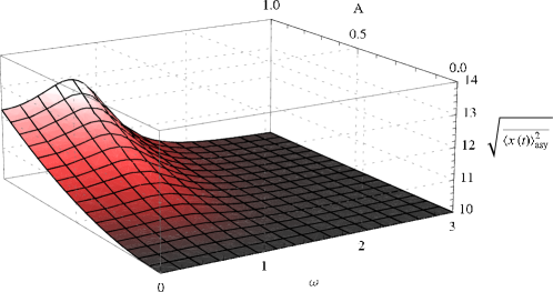
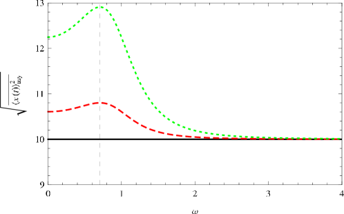
Figure 3: Upper panel: $\sqrt{\overline{\left\langle x\left(t\right)\right\rangle_{asy}^{2}}}$ vs amplitude of the heterogeneous part, $A$, and frequency, $\omega$, with $M=1$, $\gamma=1$, $k_{0}=1$, $\lambda_{0}=10$, $\bar{\Phi}=1$. The maximum, characterising a stochastic resonance phenomenon, occurs at $\omega_{\mathrm{res}}=\sqrt{\omega_{0}^{2}-2\,\theta^{2}}$ that defines the grey dashed line in the lower panel containing the plane cuts for $A=0$ (black line), $A=\frac{1}{2}$ (dashed red line) and $A=1$ (dotted green line). For this case the maximum occurs at $1/\sqrt{2}$.

Adding all the terms and taking the limit $t\rightarrow\infty$, we obtain the equilibrium energy of the system. The energy is composed of an oscillating term, with time zero average, and a constant term $E_{M}^{c}$:

$$E_{M}^{c} = \frac{1}{2}M\overline{\left\langle v\left(t\right)^{2}\right\rangle_{asy}}+\frac{1}{2}k_{0}\,\overline{\left\langle x\left(t\right)^{2}\right\rangle_{asy}}$$ (45)

$$= \lambda_{0}\frac{\bar{\Phi}^{2}}{\gamma}+\,{\frac{{\lambda_{{0}}}^{2}{\bar{\Phi}}^{2}}{2\,M\,{\omega_{{0}}^{2}}}}+{\frac{{\lambda_{{0}}}^{2}{\bar{\Phi}}^{2}{A}^{2}\left({\omega}^{2}+{\ \omega_{{0}}}^{2}\right)}{4\,M\left[\left(\omega_{0}^{2}-\omega^{2}\right)^{2}+4\,{\theta}^{2}{\ \omega}^{2}\right]}}.$$

It is worth mentioning that in this case we have made explicit the asymptotic time dependence so that our averages are computed over samples and not over time in a single sample as we have made in the previous section.

5.2 Power considerations

Going back to Eq. (43), we can define the two following quantities,

$$J_{I}=v(t)\,\eta(t),$$ (46)

and

$$J_{D}=-\gamma\,v^{2}(t).$$ (47)

Physically, both rates, $J_{I}$ and $J_{D}$, constitute changes of energy due to the interactions with the thermal bath. Within this context, it is particularly important the study of the cumulative changes of energy in the system up to a time $t=\tau$, namely the injected total,

$$J_{IT}=\int_{0}^{\tau}dt\,v(t)\,\eta(t),$$ (48)

and the dissipated total,

$$J_{DT}=-\gamma\,\int_{0}^{\tau}dt\,\,v^{2}(t).$$ (49)

in which we will apply the same Laplace transform operation in order to better handle the noise averages [18, 19, 20, 21]. The dissipation of energy flux can be written as

$$J_{DT} = -\gamma\int_{0}^{\tau}dt\,\int_{0}^{\infty}dt_{1}\,\delta(t-t_{1})\,\int_{0}^{\infty}dt_{2}\,\delta(t-t_{2})\,v(t_{1})\,\eta(t_{2}),$$

$$= \lim_{\epsilon\rightarrow 0}\int_{-\infty}^{\infty}\frac{dq_{1}}{2\pi}\,\int_{-\infty}^{\infty}\frac{dq_{2}}{2\pi}\,\frac{e^{(\mathrm{i}\,q_{1}+\mathrm{i}\,q_{2}+2\epsilon)\tau}-1}{(\mathrm{i}\,q_{1}+\mathrm{i}\,q_{2}+2\epsilon)}\,\tilde{v}(\mathrm{i}\,q_{1}+\epsilon)\,\tilde{v}(\mathrm{i}\,q_{2}+\epsilon),$$

$$= \lim_{\epsilon\rightarrow 0}\int_{-\infty}^{\infty}\frac{dq_{1}}{2\pi}\,\int_{-\infty}^{\infty}\frac{dq_{2}}{2\pi}\,\frac{e^{(\mathrm{i}\,q_{1}+\mathrm{i}\,q_{2}+2\epsilon)\tau}-1}{(\mathrm{i}\,q_{1}+\mathrm{i}\,q_{2}+2\epsilon)}\,\times$$

$$\left[\frac{(\mathrm{i}\,q_{1}+\epsilon)}{M\,R(\mathrm{i}\,q_{1}+\epsilon)}\frac{(\mathrm{i}\,q_{2}+\epsilon)}{M\,R(\mathrm{i}\,q_{2}+\epsilon)}\tilde{\eta}(\mathrm{i}\,q_{1}+\epsilon)\tilde{\eta}(\mathrm{i}\,q_{2}+\epsilon)\right],$$

which becomes, after taking the thermal average,

$$\left\langle J_{DT}\right\rangle = \left(-\frac{2\gamma\lambda_{0}\,{\bar{\Phi}}^{2}}{M^{2}}\right)\lim_{\epsilon\rightarrow 0}\int_{-\infty}^{\infty}\frac{dq_{1}}{2\pi}\,\int_{-\infty}^{\infty}\frac{dq_{2}}{2\pi}\,\frac{e^{(\mathrm{i}\,q_{1}+\mathrm{i}\,q_{2}+2\epsilon)\tau}-1}{(\mathrm{i}\,q_{1}+\mathrm{i}\,q_{2}+2\epsilon)}\,\frac{(\mathrm{i}\,q_{1}+\epsilon)}{R(\mathrm{i}\,q_{1}+\epsilon)}\frac{(\mathrm{i}\,q_{2}+\epsilon)}{R(\mathrm{i}\,q_{2}+\epsilon)}\times$$

$$\left[\frac{1}{\mathrm{i}\,q_{1}+\mathrm{i}\,q_{2}+2\,\epsilon}+\frac{A}{2}\left(\frac{1}{\mathrm{i}\,q_{1}+\mathrm{i}\,q_{2}+2\,\epsilon-\mathrm{i}\,\omega}+\frac{1}{\mathrm{i}\,q_{1}+\mathrm{i}\,q_{2}+2\,\epsilon+\mathrm{i}\,\omega}\right)\right.+$$

$$\frac{\lambda_{0}}{2}\,\left\{\frac{1}{\mathrm{i}\,q_{1}+\epsilon}+\frac{A}{2}\left(\frac{1}{\mathrm{i}\,q_{1}+\epsilon-\mathrm{i}\,\omega}+\frac{1}{\mathrm{i}\,q_{1}+\epsilon+\mathrm{i}\,\omega}\right)\right\}\times$$

$$\left.\left\{\frac{1}{\mathrm{i}\,q_{2}+2\,\epsilon}+\frac{A}{2}\left(\frac{1}{\mathrm{i}\,q_{2}+\epsilon-\mathrm{i}\,\omega}+\frac{1}{\mathrm{i}\,q_{2}+\epsilon+\mathrm{i}\,\omega}\right)\right\}\right]$$

$$\equiv J_{DT0}(\tau)+J_{D,osc}(\tau).$$

Under the condition $\tau\theta\gg 1$ (transient terms are negligible), we can explicitly write the results for the integration above as a sum of three contributions: a term proportional to $\tau$,

$$J_{DT0}(\tau)=-\left({\frac{\,{\bar{\Phi}}^{2}{\lambda_{{0}}}}{M}}+{\frac{{A}^{2}{\omega}^{2}{\bar{\Phi}}^{2}{\lambda_{{0}}^{2}\,}\theta}{\,\left[{\omega}^{2}\left(\omega^{2}-2\,{\omega_{{0}}^{2}}+4\,{\theta}^{2}\right)+{\omega_{{0}}^{2}}\right]\,M}}\right)\,\tau,$$

an oscillating term,

$$J_{D,osc}(\tau) = 8\,{\frac{A\left(3\,\theta\,{\omega}^{2}\,{\omega_{{0}}}^{2}-4\,\theta\,{\ \omega_{{0}}^{4}}-2\,\theta\,{\omega}^{4}-4\,{\theta}^{3}\,{\omega}^{2}\right){\bar{\Phi}}^{2}{\lambda_{{0}}^{2}}\gamma\sin\left(\omega\,\tau\right)}{{M}^{2}\omega\,\left(4\,{\theta}^{2}+{\omega}^{2}\right)\left({\omega}^{4}+16\,{\ {\theta}^{2}\omega}^{2}+16\,{\omega_{{0}}^{4}}-8\,{\omega}^{2}{\omega_{{0}}^{2}}\right)}}+$$ (50)

$$2\,{\frac{A\left(8\,\omega\,{\omega_{{0}}}^{4}+4\,{\theta}^{2}{\omega}^{3}+{\omega}^{5}-6\,{\omega}^{3}{\omega_{{0}}}^{2}\right)\,{\bar{\Phi}}^{2}{\lambda_{{0}}^{2}}\gamma\cos\left(\omega\,\tau\right)}{{M}^{2}\omega\,\left({\omega}^{2}+4\,{\theta}^{2}\right)\left({\omega}^{4}+16\,{\ \omega}^{2}{\theta}^{2}+16\,{\omega_{{0}}^{4}}-8\,{\omega}^{2}{\omega_{{0}}^{2}}\right)}}-$$

$$2\,{\frac{{A}^{2}\,\left[{\omega\,\theta}^{2}\sin\left(2\,\omega\,\tau\right)+\left(\,{\omega_{{0}}^{2}}\,-{\omega}^{2}\right)\cos\left(2\,\omega\,\tau\right)\right]{\bar{\Phi}}^{2}{\lambda_{{0}}^{2}}\theta^{2}\omega^{2}}{M\,\,\left[{\omega}^{2}\left(\omega^{2}-2\,{\omega_{{0}}^{2}}+4\,{\theta}^{2}\right)+{\omega_{{0}}^{2}}\right]^{2}}+}$$

$${\frac{{A}^{2}\,\left[{\omega}^{2}\left({\omega}^{4}+-2\,{\omega_{{0}}}^{2}\right)+{\omega_{{0}}}^{4}\right]{\bar{\Phi}}^{2}{\lambda_{{0}}}^{2}\theta\,\omega\,\sin\left(2\,\omega\,\tau\right)}{2\,M\,\,\left[{\omega}^{2}\left(\omega^{2}-2\,{\omega_{{0}}^{2}}+4\,{\theta}^{2}\right)+{\omega_{{0}}^{2}}\right]^{2}}},$$

and a constant term,

$$J_{DTc} = {\frac{{\bar{\Phi}}^{2}{\ \lambda_{{0}}}}{\gamma}}-{\frac{{\bar{\Phi}}^{2}{\lambda_{{0}}^{2}}}{2\,M\,{\omega_{{0}}^{2}}}}+{\frac{A{\bar{\Phi}}^{2}{\lambda_{{0}}^{2}}\left({\omega}^{2}-{\omega_{{0}}^{2}}\right)}{M\,\,\left[{\omega}^{2}\left(\omega^{2}-2\,{\omega_{{0}}^{2}}+4\,{\theta}^{2}\right)+{\omega_{{0}}^{2}}\right]}}+$$ (51)

$${\frac{{A}^{2}\left[\left[2\,{\omega}^{2}\left({\omega_{{0}}^{2}}+2\,{\theta}^{2}\right)-{\omega_{{0}}^{4}}\right]{\omega_{{0}}^{2}}+8\,\omega^{4}\,\left({\theta}^{2}-{\omega_{{0}}}^{2}\right)\right]{\bar{\Phi}}^{2}{\ \lambda_{{0}}^{2}}}{2\,M\,\left[{\omega}^{2}\left(\omega^{2}-2\,{\omega_{{0}}^{2}}+4\,{\theta}^{2}\right)+{\omega_{{0}}^{2}}\right]^{2}}},$$

where $J_{DT}=J_{DT0}(\tau)+J_{D,osc}(\tau)+J_{DTc}$.

The injection of energy can be written in a similar way,

$$J_{IT} = \int_{0}^{\tau}dt\,\int_{0}^{\infty}dt_{1}\,\delta(t-t_{1})\,\int_{0}^{\infty}dt_{2}\,\delta(t-t_{2})\,v(t_{1})\,\eta(t_{2}),$$

$$= \lim_{\epsilon\rightarrow 0}\int_{-\infty}^{\infty}\frac{dq_{1}}{2\pi}\,\int_{-\infty}^{\infty}\frac{dq_{2}}{2\pi}\,\frac{e^{(\mathrm{i}\,q_{1}+\mathrm{i}\,q_{2}+2\epsilon)\tau}-1}{(\mathrm{i}\,q_{1}+\mathrm{i}\,q_{2}+2\epsilon)}\,\tilde{v}(\mathrm{i}\,q_{1}+\epsilon)\,\tilde{\eta}(\mathrm{i}\,q_{2}+\epsilon),$$

$$= \lim_{\epsilon\rightarrow 0}\int_{-\infty}^{\infty}\frac{dq_{1}}{2\pi}\,\int_{-\infty}^{\infty}\frac{dq_{2}}{2\pi}\,\frac{e^{(\mathrm{i}\,q_{1}+\mathrm{i}\,q_{2}+2\epsilon)\tau}-1}{(\mathrm{i}\,q_{1}+\mathrm{i}\,q_{2}+2\epsilon)}\,\left[\frac{(\mathrm{i}\,q_{1}+\epsilon)}{M\,R(\mathrm{i}\,q_{1}+\epsilon)}\tilde{\eta}(\mathrm{i}\,q_{1}+\epsilon)\tilde{\eta}(\mathrm{i}\,q_{2}+\epsilon)\right],\,$$

where after taking the thermal average gives,

$$\left\langle J_{IT}\right\rangle = \left(\frac{\lambda_{0}\,\overline{\Phi^{2}}}{M}\right)\lim_{\epsilon\rightarrow 0}\int_{-\infty}^{\infty}\frac{dq_{1}}{2\pi}\,\int_{-\infty}^{\infty}\frac{dq_{2}}{2\pi}\,\frac{e^{(\mathrm{i}\,q_{1}+\mathrm{i}\,q_{2}+2\epsilon)\tau}-1}{(\mathrm{i}\,q_{1}+\mathrm{i}\,q_{2}+2\epsilon)}\,\frac{(\mathrm{i}\,q_{1}+\epsilon)}{R(\mathrm{i}\,q_{1}+\epsilon)}\times$$

$$\left[\frac{1}{\mathrm{i}\,q_{1}+\mathrm{i}\,q_{2}+2\,\epsilon}+\frac{A}{2}\left(\frac{1}{\mathrm{i}\,q_{1}+\mathrm{i}\,q_{2}+2\,\epsilon-\mathrm{i}\,\omega}+\frac{1}{\mathrm{i}\,q_{1}+\mathrm{i}\,q_{2}+2\,\epsilon+\mathrm{i}\,\omega}\right)\right.+$$

$$+ \frac{\lambda_{0}}{2}\,\left\{\frac{1}{\mathrm{i}\,q_{1}+\epsilon}+\frac{A}{2}\left(\frac{1}{\mathrm{i}\,q_{1}+\epsilon-\mathrm{i}\,\omega}+\frac{1}{\mathrm{i}\,q_{1}+\epsilon+\mathrm{i}\,\omega}\right)\right\}\times$$

$$\times \left.\left\{\frac{1}{\mathrm{i}\,q_{2}+2\,\epsilon}+\frac{A}{2}\left(\frac{1}{\mathrm{i}\,q_{2}+\epsilon-\mathrm{i}\,\omega}+\frac{1}{\mathrm{i}\,q_{2}+\epsilon+\mathrm{i}\,\omega}\right)\right\}\right]$$

$$\equiv J_{IT0}(\tau)+J_{IT,osc}(\tau)+J_{ITc}.$$

An important part of the injection of energy flux has to be carefully obtained since,

$$\left\langle J_{IT0}(\tau)\right\rangle_{1} = \frac{\lambda_{0}\,\overline{\Phi^{2}}}{M}\lim_{\epsilon\rightarrow 0}\int_{-\infty}^{\infty}\frac{dq_{1}}{2\pi}\,\int_{-\infty}^{\infty}\frac{dq_{2}}{2\pi}\,\frac{e^{(iq_{1}+iq_{2}+2\epsilon)\tau}-1}{(\mathrm{i}\,q_{1}+\mathrm{i}\,q_{2}+2\epsilon)^{2}}\,\frac{(\mathrm{i}\,q_{1}+\epsilon)}{R(\mathrm{i}\,q_{1}+\epsilon)}$$

$$= \frac{\lambda_{0}\,\overline{\Phi^{2}}}{M}\,\tau\lim_{\epsilon\rightarrow 0}\int_{-\infty}^{\infty}\frac{dq_{1}}{2\pi}\,\,\left(\frac{(\mathrm{i}\,q_{1}+\epsilon)}{(\mathrm{i}\,q_{1}+\epsilon-\kappa_{+})(\mathrm{i}\,q_{1}+\epsilon-\kappa_{-})}\right),$$

$$= \frac{\lambda_{0}\,\overline{\Phi}^{2}}{\,M}\tau,$$

where the last term in the r.h.s. contains the integration over the the upper arch, because the reduction lemma is not valid in this case, and using the relations between raw moments of $\Phi$ as well.

Then finally, we write the contributions for the injection of energy as

$$J_{IT0}(\tau)=\left(\frac{\lambda_{0}\,{\bar{\Phi}}^{2}}{\,M}+{\frac{{A}^{2}{\omega}^{2}\,\theta\,{\lambda_{{0}}^{2}\,\bar{\Phi}}^{2}}{M\,\left[{\omega}^{2}\left(\omega^{2}-2\,{\omega_{{0}}^{2}}+4\,{\theta}^{2}\right)+{\omega_{{0}}^{4}}\right]}}\right)\,\tau,$$

and

$$J_{IT,osc}(\tau) = {\frac{\lambda_{{0}}{\bar{\Phi}}^{2}A\sin\left(\omega\,\tau\right)}{M\omega}}+{\frac{A\left[A\left({\omega_{{0}}}^{2}-{\omega}^{2}\right)\,\cos\left(2\,\omega\,\tau\right)+4\,{\omega_{{0}}}^{2}\cos\left(\omega\,\tau\right)\right]{\lambda_{{0}}^{2}\,\bar{\Phi}}^{2}}{4\,M\,\left[{\omega}^{2}\left(\omega^{2}-2\,{\omega_{{0}}^{2}}+4\,{\theta}^{2}\right)+{\omega_{{0}}^{4}}\right]}}$$ (52)

$$+{\frac{A\left[2\omega\theta\left(A\sin\left(2\,\omega\,\tau\right)+4\sin\left(\omega\,\tau\right)\right)-4\,{\omega}^{2}\cos\left(\omega\,\tau\right)\right]{\lambda_{{0}}^{2}\,\bar{\Phi}}^{2}}{4\,M\,\left[{\omega}^{2}\left(\omega^{2}-2\,{\omega_{{0}}^{2}}+4\,{\theta}^{2}\right)+{\omega_{{0}}^{4}}\right]},}$$

and

$$J_{ITc} = {\frac{{\lambda_{{0}}^{2}\bar{\Phi}}^{2}}{M{\omega_{{0}}^{2}}}}+{\frac{A{\lambda_{{0}}^{2}\bar{\Phi}}^{2}\left({\omega_{{0}}}^{2}-{\omega}^{2}\right)}{M\,\left[{\omega}^{2}\left(\omega^{2}-2\,{\omega_{{0}}^{2}}+4\,{\theta}^{2}\right)+{\omega_{{0}}^{4}}\right]}}+$$ (53)

$$\,{\frac{\left[{\omega}^{4}\left({\omega}^{2}-12\,{\theta}^{2}\right)+{\omega_{{0}}^{2}}\left(3\,{\omega_{{0}}^{4}}-5\,{\omega_{{0}}^{2}\,\omega}^{2}+{\omega}^{4}-4\,{\theta}^{2}\right)\right]\,{A}^{2}{\lambda_{{0}}^{2}\,\bar{\Phi}}^{2}}{4\,M\,\left[{\omega}^{2}\left(\omega^{2}-2\,{\omega_{{0}}^{2}}+4\,{\theta}^{2}\right)+{\omega_{{0}}^{4}}\right]^{2}}}.$$

For the total energy flux $J_{E}=J_{IT}+J_{DT}$ it can be easily seen that the linear term on $\tau$ cancel out, while the constant term becomes exactly the average energy of Eq. (45). The non-oscillating part of the energy reads,

$$J_{E}^{no}=\,{\frac{{\bar{\Phi}}^{2}\lambda_{{0}}\left(2\,M{\omega_{{0}}}^{2}+\lambda_{{0}}\gamma\right)}{2\gamma\,M{\omega_{{0}}^{2}}}}+{\frac{\left({\omega}^{2}+{\omega_{{0}}}^{2}\right){A}^{2}{\bar{\Phi}}^{2}{\lambda_{{0}}}^{2}}{4\,M\,\left[{\omega}^{2}\left(\omega^{2}-2\,{\omega_{{0}}^{2}}+4\,{\theta}^{2}\right)+{\omega_{{0}}^{4}}\right]}},$$ (54)

coinciding perfectly with Eq. (45). The oscillating term $J_{IT,osc}+J_{DT,osc}$ do not contribute if the time average is taken. Thus, the average energy will in the form of an oscillation around the mean.

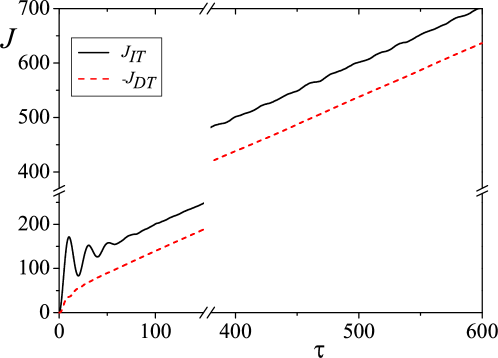
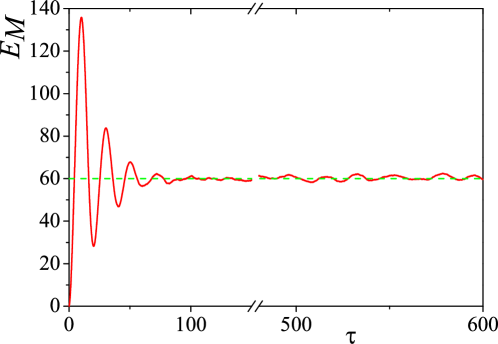
Figure 4: Upper panel: Total injected and (symmetric) dissipated power, $J_{IT}\left(-J_{DT}\right)$ vs time, $\tau$, according to the definitions in the legend. Lower panel: Total energy, $E_{M}$, vs time, $\tau$. The dashed (green) line represents the assymptotic limit given by Eq. (45). In both cases we have used the following values: $M=10$, $k_{0}=1$, $\gamma=1$ $\bar{\Phi}=1$, $\lambda_{0}=10$ and $A=0$. n.b.: The difference between the values of $J_{IT}$ and $-J_{DT}$ in the upper panel is exactly equal to the total energy, $E_{M}$, that is shown in the lower panel and equals the theoretical value given by Eq. (45) as well.

As expected, in the long-term the magnitudes of the injected and dissipated energy fluxes are exactly the same signalling the emergence of equilibrium. All of our calculations are compatible with the plots in Fig. 4 whereby we depict the evolution of the injected and dissipated power total (mechanical) energy of an oscillator following our dynamical equations.

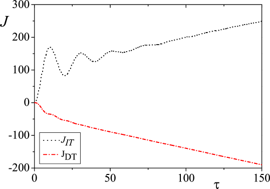
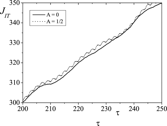
Figure 5: Upper panel: Total injected, $J_{IT}$, and dissipated power, $J_{DT}$, vs time, $\tau$, according to the definitions in the legend for the heterogeneous case $M=10$, $k_{0}=1$, $\gamma=1$ $\bar{\Phi}=1$, $\lambda_{0}=10$ and $A=1/2$. Lower panel: Comparison of $J_{IT}$ for this heterogeneous process with a homogeneous process ($A=0$) under the same remaining parameters. The impact of the oscilations in the noise are clearly visible.

6 Concluding remarks

In this work we have revisited the problem of the damped harmonic oscillator subject to a heterogeneous Poisson process. Our approach, which is carried out by averaging over the noise in the Fourier-Laplace space, allowed us to obtain the long-term distributions of the position and distributions (joint and marginal). Moreover, we have surveyed the interaction between the system and the thermal bath by computing the rates of energy that are dissipated from the system and injected into it. As expected, after a transient time, both rates balance so that the system achieves a steady state. The application of time averages over the position and velocity of the massive partible has allowed obtaining the long-term distributions of the two quantities, which is independent of the heteregeneous character of the noise. This last feature will only have impact when averages over samples, instead of averages of the time, are implemented. Notwithstanding, we having been able to find the effect of the heterogeneity of the rate of events be the emergence of resonance effects linking the “natural” frequency of oscillation and and the frequency of the time-dependent part of the rate of events. This impact is also visible when the total injected and dissipated powers have been surveyed. Considerations regarding Jarzynski’s equalities as well as modifications on the inter-event rule of the noise are addressed to future work.

Appendix A Numerical calculations

In order to solve in a numerical way our main Eqs. (1) and (2) we have considered a trapezoidal approximation which is reminiscent of the Stratanovich approach to noise phenomena,

$$x\left(t_{2}\right)-x\left(t_{1}\right)=\int_{t_{1}}^{t_{2}}v\left(t\right)\,dt\approx\left(t_{2}-t_{1}\right)\frac{v\left(t_{2}\right)+v\left(t_{1}\right)}{2},$$

and the same for the deterministic part of the velocity,

$$\Delta v^{\det}\left(t_{2},t_{1}\right) \equiv M^{-1}\int_{t_{1}}^{t_{2}}\left[-k_{0}x(t)-\gamma v(t)\right]dt$$

$$\approx \left(t_{1}-t_{2}\right)\frac{\gamma\left[v\left(t_{2}\right)+v\left(t_{1}\right)\right]+k_{0}\left[x\left(t_{2}\right)+x\left(t_{1}\right)\right]}{2\,M},$$

for small enough $dt$.

In respect of the stochastic part [24], its calculation can be at least made threefold. The first one concerns the inter-event time which is given by Eq. (9). Accordingly, starting from $t_{0}$ we would randomly select a certain time interval, $\delta t$, following PDF in Eq. (9) and we would let deterministic equations evolve up to $t_{0}+\delta t$ when we would add the value of the kick, $M^{-1}\Phi\left(t_{0}+\delta t\right),$ to $\Delta v^{\det}$ with $\Phi$ chosen from the specific distribution $P\left(\Phi\right)$. Despite its accurateness this procedure is not the most hard-headed when it comes to simulating heterogeneous Poisson processes, since we are obliged to constantly update the distribution in a rather grinding way.

The second method is a shrewd procedure of carrying out the numerical simulation without having to heed to a very tiny value of the mesh $\delta t$ or also to problems with a very high rate of occurrence of events $\lambda\left(t\right)$. In this case we can determine the (expected) number of events that take place within $\delta t$,

$$n\left(t\right)=\int_{t}^{t+\delta t}\lambda\left(t^{\prime}\right)\,dt^{\prime},$$

and consider that the overall effect of the noise in that time interval is equivalent to the occurrence of a single kick the intensity of which is given by the convolution of $n\left(t\right)$ distributions $P\left(\Phi\right)$. Bearing in mind that the events are uncorrelated the resulting distribution is given by,

$$P_{n}\left(\Phi\right)=\mathcal{F}_{\Phi}^{-1}\left[\mathcal{F}_{\phi}\left[P\left(\Phi\right)\right]^{n}\right].$$

However, it must be stressed that this procedure is half-averaged since it already assumes the mean number of events in its implementation, thus leaving all the randomness to the resulting amplitude of the added noise. Although we have not tested the following assertation, we believe that its application reduces the number of samples needed to obtain the same dispersion in the sample set.

The third way corresponds to our main option, particularly for the figures in the text. Specifically, we were intentionally careless about optimising computational time, as we have preferred a very conservative approach and a very tight grid. Since we did not opt for depicting examples with very high event rates, we went ahead by picking a random number uniformly distributed between 0 and 1 and compared it with the probability of having an event according with the Poisson distribution with parameter $\int_{t}^{t+\delta t}\lambda\left(t^{\prime}\right)\,dt^{\prime}$, which is similar to Eq. (12). If the random number is the smaller of both numbers, then a kick takes place and therefore we need to select the noise intensity as described for the first approach. In all the cases we have shown $\delta t=10^{-4}$. The distributions were obtained from a total of $5\times 10^{8}$ records (10³ samples) made at intervals of $10^{-3}$ time units. To assure equilibrium we have set apart the first 10⁵ (100 time units) logs of each sample.

References

References

- [1] N C van Kampen. Stochastic processes in Physics and Chemistry. North-Holland, Amsterdam, 1992.
- [2] P Hänggi and F Marchesoni. Artificial Brownian motors: Controlling transport on the nanoscale. Reviews of Modern Physics, 81(1):387–442, 2009.
- [3] W E Leland, M S Taqqu, W Willinger, and D V Wilson. On the self-similar nature of Ethernet traffic (extended version). IEEE/ACM Transactions on Networking, 2(1):1–15, 1994.
- [4] N G van Kampen. How good is Langevin. The Journal of Physical Chemistry. B, 109(45):21293–5, 2005.
- [5] E Nelson. Dynamical Theories of Brownian Motion. Princeton University Press, Princeton, 2006, 2nd Ed. also available at: www.math.princeton.edu/nelson/books.html.
- [6] N G van Kampen and I Oppenheim. Brownian motion as a problem of eliminating fast variables. Physica A, 138:231, 1986.
- [7] K Ioannis and S E Shreve. Brownian Motion and Stochastic Calculus. Springer-Verlag, New York, 1991, 2nd Ed.
- [8] D Revuz and M Yor. Continuous martingales and Brownian motion. Springer-Verlag, 1994, 2nd Ed.
- [9] J-P Bouchaud and A Georges. Anomalous diffusion in disordered media: Statistical mechanisms, models and physical applications. Physics Reports, 195(4-5):127–293, 1990.
- [10] A Baule and E G D Cohen. Fluctuation properties of an effective nonlinear system subject to Poisson noise. Physical Review E, 79(3):30103, 2009.
- [11] C Anteneodo, R D Malmgren, and D R Chialvo. Poissonian bursts in e-mail correspondence. The European Physical Journal B, 75(3):389–394, 2010.
- [12] M I Dykman. Poisson-noise-induced escape from a metastable state. Physical Review E, 81(5):51124, 2010.
- [13] P Hanggi, K E Shuler, and I Oppenheim. On the relations between markovian master equations and stochastic differential equations. Physica A, 107(A):143 – 157, 1981.
- [14] R Benzi, A Sutera, and A Vulpiani. The mechanism of stochastic resonance. J. Phys. A: Math. and Gen., 14:L453, 1981.
- [15] J R Chaudhuri, P Chaudhuri, and S Chattopadhyay. Harmonic oscillator in presence of nonequilibrium environment. J. Chem. Phys., 130:234109, 2009.
- [16] A Eusebio, A Pogosyan, S Wang, B Averbeck, L D Gaynor, S Cantiniaux, T Witjas, T Limousin, J-P Azulay, and P Brown. Resonance in subthalamo-cortical circuits in Parkinson’s disease. Brain, 132:2139, 2009.
- [17] C Stambaugh and H B Chan. Noise-activated switching in a driven nonlinear micromechanical oscillator. Physical Review B, 74:172302, 2006.
- [18] D O Soares-Pinto and W A M Morgado. Brownian dynamics, time-averaging and colored noise. Physica A, 365:289, 2006.
- [19] D O Soares-Pinto and W A M Morgado. Exact time-average distribution for a stationary non-Markovian massive Brownian particle coupled to two heat baths. Physical Review E, 77:011103, 2008.
- [20] W A M Morgado and D O Soares-Pinto. Exact time-averaged thermal conductance for small systems: Comparison between direct calculation and Green-Kubo formalism. Physical Review E, 79:051116, 2009.
- [21] W A M Morgado and D O Soares-Pinto. Exact Nonequilibrium Work Generating Function for a Small Classical System. Physical Review E, 82:021112, 2010.
- [22] J F C Kingman. Poisson Processes (Oxford Studies in Probability). Clarendon Press, Oxford, 1992.
- [23] P Reimann, R Bartussek, R Häussler, and P Hänggi. Brownian motors driven by temperature oscillations. Physics Letters A, 215:26, 1996.
- [24] C Kim, E K Lee, P Hänggi, and P Talkner. Numerical method for solving stochastic differential equations with Poissonian white shot noise. Phys. Rev. E, 76:011109, 2007.