IPM/P-2011/017

On Holography of Julia-Zee Dyon

Davood Allahbakhshi

Department of Physics, Sharif University of Technology
P.O. Box 11365-9161, Tehran, Iran

School of physics, Institute for Research in Fundamental Sciences (IPM)
P.O. Box 19395-5531, Tehran, Iran

allahbakhshi@ipm.ir

The holographic dual of self gravitating Julia-Zee dyon is discussed. It is shown that the dual field theory is generally a field theory with a vortex condensate. The vacuum expectation values of the dual operators, as functions of the sources in the field theory, are studied in a class of bulk solutions. In these solutions the sign of the vacuum expectation values of the dual operators change, by changing the sources in the model.

1 Introduction

It is well known that the AdS/CFT correspondence [1, 2, 3], is a useful tool in understanding at least the qualitative features of strongly coupled field theories. During past years many holographic models are studied. In some cases the bulk theories are constructed so as to simulate certain features of a known quantum field theory, e.g., AdS/QCD and AdS/CMT models; and in some cases a field theory is proposed as the dual theory of a given bulk theory. In both approaches, by the well known recipe of AdS/CFT correspondence, the key considerations are symmetries and the field contents of the theories. In some cases the comparable quantities and behaviors are illuminating for finding the dual theories.

In this work we study one of the gravitational systems recently studied, the self gravitating Julia-Zee dyon [4, 5, 6]. A.R.Lugo, E.F.Moreno and F.A.Schaponsik, have found a numerical solutions for the Julia-Zee black dyon, in the BPS limit, with[5] and without[4] back reaction on the metric, and they found that the vacuum expectation values vanish by raising the temperature of the bulk blackhole. It can be considered as a phase transition from a dyonic blackhole. In [6], it is shown that a simple, vanishing scalar solution for the dyon, becomes dynamically unstable by lowering the temperature of the bulk blackhole to a scalar hairy blackhole, which means that the dual field theory changes its vacuum, so by lowering the temperature of the dual boundary system, a phase transition occurs to a scalar condensed phase. Multimonopole solutions with AdS background are studied with axial [7, 8] and crystalline [9, 10] symmetry. In[9], D.Tong and S.Bolognesi have studied the multi monopole solution at the BPS limit, and found that at low temperatures, the multi monopole solutions are favored in comparison to blackhole single monopole solutions. As the multi monopole solutions in AdS background can have crystalline symmetry, they have proposed that these configurations could correspond to strange metals at low temperatures. In this article we study the holographic vacuum expectation values for the dual operators, by the well known recipe of the Gauge/Gravity duality; and also calculate a numerical solution to the equations of motion, to determine the behavior of the v.e.vs of the dual operators, as functions of the sources.

The paper is organized as follows. In the next section we introduce the bulk action, equations of motion and the form of the Julia-Zee dyon. In section (3) we calculate the vacuum expectation values of the dual operators, generally from Einstein-Yang-Mills-Higgs action and as a special case, for Julia-Zee dyon. In section (4) we find a set of numerical solutions for the dyon, and generically study their thermodynamics and v.e.v of the dual operators. In the last section we end with conclusion.

2 The model

The action we consider in this article is [6]:

$$S\ =\int\sqrt{-g}\;d^{4}x\ \big{[}\frac{1}{16\pi G}(R+\frac{6}{L^{2}})-\frac{1}{4}F^{a}_{\mu\nu}F^{a\mu\nu}-\frac{1}{2}D_{\mu}\phi^{a}D^{\mu}\phi^{a}-\frac{\lambda}{4}(\phi^{a}\phi^{a})^{2}+\frac{1}{L^{2}}(\phi^{a}\phi^{a})\big{]},$$ (2.1)

The covariant derivative and the field strength are:

$$D_{\mu}\phi^{a}=\partial_{\mu}\phi^{a}+e\epsilon^{abc}A^{b}_{\mu}\phi^{c}\;;\;F^{a}_{\mu\nu}=\partial_{\mu}A^{a}_{\nu}-\partial_{\nu}A^{a}_{\mu}+e\epsilon^{abc}A^{b}_{\mu}A^{c}_{\nu}.$$ (2.2)

As is clear, the mass term for the scalar field is chosen to be $m^{2}=-2/L^{2}$. Since the su(2) gauge symmetry of the bulk action corresponds to a global su(2) symmetry in dual field theory, so the scalar field can be considered as the dual of a two fermion flavored composite operator (similar to pions or a flavored Cooper pair). In this sense, since the mass dimension of a fermion in 2+1 dimensions is one, the operator dual to the $\phi$, in the field theory, will have mass dimension two. On the other hand the source that couples to such an operator has mass dimension one. In order to have these special mass dimensions, the asymptotic form of the bulk scalar field should be:

$$\phi=\frac{\tilde{\phi}_{0}}{r}+\frac{\tilde{\phi}_{1}}{r^{2}}+...\;.$$ (2.3)

So $m^{2}$, has to be $-2/L^{2}$.

The equations of motion are:

$$\begin{split}&R_{\mu\nu}-\frac{1}{2}(R+\frac{6}{L^{2}})\;g_{\mu\nu}=8\pi G\;T_{\mu\nu}\cr&T_{\mu\nu}=\big{[}-\frac{1}{4}F_{\rho\lambda}^{a}F^{a\rho\lambda}-\frac{1}{2}D_{\lambda}\phi^{a}D^{\lambda}\phi^{a}-V(\phi^{2})\big{]}g_{\mu\nu}+F^{a}_{\mu\lambda}F^{a\lambda}_{\nu}+D_{\mu}\phi^{a}D_{\nu}\phi^{a}\cr\cr&D_{\mu}\big{(}\sqrt{-g}D^{\mu}\phi\big{)}^{a}-\sqrt{-g}\;\frac{\delta V}{\delta\phi^{a}}=0\cr\cr&D_{\mu}\big{(}\sqrt{-g}F^{\mu\nu}\big{)}^{a}-e\sqrt{-g}\;\epsilon^{abc}\;\phi^{b}\;(D^{\nu}\phi)^{c}=0\end{split}$$ (2.4)

The Julia-Zee ansatz has the form:

$$\begin{split}\phi=\vec{\sigma}.\vec{\phi}&=\frac{H(r)}{er}\;\sigma^{r}\cr A=\vec{\sigma}.\vec{A}&=\frac{J(r)}{er}\;\sigma^{r}\;dt+\frac{1-K(r)}{e}\;\big{(}-\sigma^{\varphi}\;d\theta+sin(\theta)\;\sigma^{\theta}\;d\varphi\big{)},\end{split}$$ (2.5)

where $\sigma^{r},\sigma^{\theta},\sigma^{\varphi}$ are defined as:

$$\sigma^{r}=\hat{r}.\vec{\sigma}\;,\;\sigma^{\theta}=\hat{\theta}.\vec{\sigma}\;,\;\sigma^{\varphi}=\hat{\varphi}.\vec{\sigma}$$ (2.6)

and $\hat{r}\;,\;\hat{\theta}\;,\;\hat{\varphi}$ are the usual unit vectors of spherical coordinates . We consider the metric in the most general form of a spherical symmetric metric in global coordinates:

$$ds^{2}=\;-e^{X(r)}\;dt^{2}\;+\;e^{Y(r)}\;dr^{2}\;+\;r^{2}\;d\Omega_{2}^{2}$$ (2.7)

There are two simple solutions for the full equations of motion [11, 6]:

$$\begin{split}H&=Cr\;,\;K=0\;,\;J=\mu r-\rho\;,\;e^{X}=e^{-Y}=1-\frac{2M}{r}+\frac{q^{2}}{r^{2}}+\frac{r^{2}}{\tilde{L}^{2}}\cr H&=0\;,\;K=0\;,\;J=\mu r-\rho\;,\;e^{X}=e^{-Y}=1-\frac{2M}{r}+\frac{q^{2}}{r^{2}}+\frac{r^{2}}{L^{2}}\end{split}$$ (2.8)

where $C=\sqrt{2/\lambda L^{2}}$ is the minimum of the potential, and q is related to $\rho$ through:

$$q^{2}=\frac{4\pi G_{N}(1+\rho^{2})}{e^{2}},$$ (2.9)

and $\rho$ is related to the chemical potential by

$$\rho=\mu r_{H}.$$ (2.10)

$\tilde{L}$ satisfies:

$$\frac{1}{\tilde{L}^{2}}=\frac{1}{L^{2}}+\frac{8\pi G_{N}}{3\lambda L^{4}}.$$ (2.11)

It is very easy to see that for the above solution there is a relation between the temperature of the blackhole and chemical potential as:

$$T+\alpha\;\mu^{2}=\beta$$ (2.12)

where $\alpha$ and $\beta$ are two constants related to the parameters of the solution ($\lambda,r_{H},G_{N},e,L$). This relation is in fact the first law of thermodynamics:

$$\frac{\epsilon+P}{s}=T+\mu\;\frac{\rho}{s}\;;\;\rho\propto\mu$$ (2.13)

3 Vacuum of dual theory

To understand the vacuum of the dual field theory, we should calculate the vacuum expectation values of the operators in the field theory. In the theory under consideration we have a scalar field, $\phi^{a}$, which is dual to a scalar operator, $O^{a}$, and a gauge field $A^{a}_{\mu}$, which corresponds to a vector operator, $V^{a}_{\mu}$, in the dual field theory.

Before we proceed to calculate the one point functions of the operators, we recall the linear method for calculating them in AdS/CFT.

Suppose that we have a bulk theory which is defined by an action S($\phi$). In order to calculate the 1-point functions we need to vary the on-shell action with respect to the fields. Expanding to the second order we have:

$$\begin{split}S_{on-shell}(\phi_{B}+\delta\phi)&=S^{(0)}(\phi_{B})+S^{(1)}(\phi_{B},\delta\phi)+S^{(2)}(\phi_{B},\delta\phi^{2})+...;\end{split}$$ (3.1)

the first term is the free energy of the dual theory. The second and third terms can be written in the forms:

$$\begin{split}S^{(1)}&=\int{\delta\phi.(\text{b.e.m})}+\;S_{N}^{(1)}(\phi_{B},\delta\phi)\cr S^{(2)}&=\int{\delta\phi.(\text{f.e.m})}+\;S_{N}^{(2)}(\phi_{B},\delta\phi^{2})\end{split}$$ (3.2)

the terms b.e.m and f.e.m refer to the expressions for the background equation of motion and that of the linearized equation of motion for the fluctuation, respectively; which are zero. Now suppose that the asymptotic expansion of the fields are:

$$\begin{split}\phi_{B}&=\tilde{\phi}_{s}r^{\Delta_{+}}+...+\tilde{\phi}_{c}r^{\Delta_{-}}+...,\cr\delta\phi&=\delta\tilde{\phi}_{p}r^{\Delta_{+}}+...+\delta\tilde{\phi}_{r}r^{\Delta_{-}}+...,\end{split}$$ (3.3)

where the subscripts s,c,p,r, refer to source, condensate, probe and response, respectively.

In general the relevant parts of the $S_{N}$’s are of the forms:

$$\begin{split}S_{N}^{(1)}&=\int{...+\;c_{B}\;\delta\tilde{\phi}_{p}\;\tilde{\phi}_{c}}\;+...\cr S_{N}^{(2)}&=\int{...+\;c_{r}\;\delta\tilde{\phi}_{p}\;\delta\tilde{\phi}_{r}}\;+...\end{split}$$ (3.4)

where cs are constants. Then the one point function for the operator dual to $\phi$ will be:

$$\langle O\rangle=\frac{\delta S_{on-shell}}{\delta\tilde{\phi}_{p}}=c_{B}\;\tilde{\phi}_{c}+c_{r}\;\delta\tilde{\phi}_{r}=\langle O\rangle_{B}+\langle O\rangle_{r},$$ (3.5)

where subscripts B and r refer to the background contribution to the v.e.v of O, and the response of the system to the probe, respectively.

Doing the above calculation for the Einstein-Yang-Mills-Higgs action leads to:

$$\begin{split}S(A_{B}+\delta A,\phi_{B}+\delta\phi)=&S^{(0)}(A_{B},\phi_{B})+\cr&S_{\phi}^{(1)}(A_{B},\phi_{B},\delta\phi)+S_{A}^{(1)}(A_{B},\phi_{B},\delta A)+\cr&S_{\phi}^{(2)}(A_{B},\phi_{B},\delta\phi^{2})+S_{A\phi}^{(2)}(A_{B},\phi_{B},\delta A,\delta\phi)+S_{A}^{(2)}(A_{B},\phi_{B},\delta A^{2})+...\cr=&S^{(0)}(A_{B},\phi_{B})+\cr&S_{N\phi}^{(1)}(A_{B},\phi_{B},\delta\phi)+S_{NA}^{(1)}(A_{B},\phi_{B},\delta A)+\cr&S_{N\phi}^{(2)}(A_{B},\phi_{B},\delta\phi^{2})+S_{NA}^{(2)}(A_{B},\phi_{B},\delta A^{2})+...;\end{split}$$ (3.6)

In the last line we have used the equations of motion for background and linear equations for fluctuations. For Einstein-Yang-Mills-Higgs action, the Noether actions are:

$$\begin{split}S^{(1)}_{N\phi}&=-\int{\sqrt{-g}\;\delta\vec{\phi}.D^{\mu}\vec{\phi_{B}}\;ds_{\mu}}=-\int{\sqrt{-g}\;\delta\vec{\phi}.D^{r}\vec{\phi_{B}}\;d^{3}x}\cr S^{(2)}_{N\phi}&=-\frac{1}{2}\int{\sqrt{-g}\;\delta\vec{\phi}.D^{\mu}\delta\vec{\phi}\;ds_{\mu}}=-\frac{1}{2}\int{\sqrt{-g}\;\delta\vec{\phi}.D^{r}\delta\vec{\phi}\;d^{3}x}\cr S^{(1)}_{NA}&=-\int{\sqrt{-g}\;\delta\vec{A}_{\nu}.\vec{F}_{B}^{\mu\nu}\;ds_{\mu}}=-\int{\sqrt{-g}\;\delta\vec{A}_{\nu}.\vec{F}_{B}^{r\nu}\;d^{3}x}\cr S^{(2)}_{NA}&=-\frac{1}{2}\int{\sqrt{-g}\;\delta\vec{A}_{\nu}.\delta\vec{F}^{\mu\nu}\;ds_{\mu}}=-\frac{1}{2}\int{\sqrt{-g}\;\delta\vec{A}_{\nu}.\delta\vec{F}^{r\nu}\;d^{3}x}\end{split}$$ (3.7)

where $ds_{\mu}$ is the area element normal to the boundary.

So roughly we have:

$$\langle\vec{V}_{\mu}\rangle_{B}\propto(\vec{F}_{B})_{r\mu}\;,\;\langle\vec{O}\rangle_{B}\propto\partial_{r}\vec{\phi}_{B}.$$ (3.8)

The v.e.v of the charge density operator ($V_{0}=\rho$), is proportional to the radial electric field; the v.e.v of spatial components of the vector operator ($V_{i}$), are proportional to the tangent to the boundary components of the magnetic field, and the v.e.v of the scalar operator is proportional to the radial derivative of the scalar field. So for Enstein-Yang-Mills-Higgs action, the radial magnetic field, which is the characteristic of magnetic monopoles, doesn’t contribute to v.e.vs as a condensate; but, its boundary value plays the role of a source for the dual field theory. If we want the radial magnetic field to contribute to the v.e.vs, as a condensate, we have to add other terms to the action. For example adding a $\theta$-term leads to:

$$\begin{split}\langle\vec{\rho}\rangle&\propto\vec{E}_{r}+\theta\;\vec{B}_{r}\cr\langle\vec{V}_{i}\rangle&\propto\epsilon_{ij}\;(\vec{B}_{j}+\theta\;\vec{E}_{j})\end{split}$$ (3.9)

3.1 Julia-Zee dyon and Vortex condensation

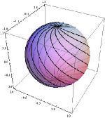
(a)

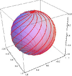
(b)

Figure 1: plot of directed curves for $e_{+}$ (a) and $e_{-}$ (b) basis.

Applied to the Julia-Zee dyon, it is easy to see that:

$$\langle\vec{V}_{t}\rangle\propto(\vec{E})_{r}\propto(\frac{J}{r})^{\prime}\;\hat{r}$$ (3.10)

$$\langle\vec{V}_{i}\rangle\propto\epsilon_{ij}(\vec{B})_{j}\propto K^{\prime}\;\epsilon_{ij}\partial_{j}\hat{r}$$ (3.11)

$$\langle\vec{O}\rangle\propto\partial_{r}\vec{\phi}\propto(\frac{H}{r})^{\prime}\;\hat{r}.$$ (3.12)

Thus for both solutions in (2.7), these quantities are zero, except for the charge density. In the next section we will introduce a numerical set of solutions for which the vacuum expectation value of the operators are non zero, and we will study them in the phase space; but, before we proceed, it is interesting to look at the profile of the vector condensate.

By looking at the ansatz (2.4), we see that only two components of the vector field are non zero, $A_{\theta}^{\varphi}$ and $A_{\varphi}^{\theta}$; where the subscripts refer to spatial indices and superscripts are internal indices. Projecting this vector on the surface, by stereographic projection, we see that the profile of the vector is that of a vortex. These vectors do not have definite charge under $\sigma^{r}$; but, after some simple algebra we can change the basis to have definite charge vectors. As usual we can define $\tau^{\pm}=\tau^{\theta}\pm i\tau^{\varphi}$ and write

$$A=\frac{2J}{er}\;\tau^{r}\;dt+\;\frac{1-K}{e}\big{[}\tau^{+}\;\hat{e}_{+}+\tau^{-}\;\hat{e}_{-}\big{]}$$ (3.13)

where the $\hat{e}_{\pm}$ are:

$$\hat{e}_{\pm}=sin(\theta)\;d\varphi\;\pm\;i\;d\theta.$$ (3.14)

As it is clear, by multiplying these basis with a length factor R, the real part of the basis is the azimuthal and the imaginary part of the basis is radial differential length elements in the complex plane. In figure (1) we have shown the directed curves for $e^{\pm}$ basis. At the poles the basis is completely polar, and at the equator there are equal contributions to the $\hat{e}_{\pm}$, from $\theta$ and $\varphi$ coordinates. The profile of the vector in this basis is also similar to a vortex. In hedgehog gauge the magnetic charge is related to $\pi_{2}(S^{2})$, but, in abelian gauge it is the magnetic flow which is carried by the Dirac string[12]; since the Dirac string passes through the center of the vortex, so the magnetic charge is the magnetic flow which is trapped by the vortex. In figure (2), we have shown the profile of the vector condensate, in hedgehog gauge.

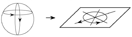
Figure 2: profile of the vector condensate.

4 Numerical calculations

In this section we construct a numerical self-garvitating Julia-Zee dyon, and study the behavior of the v.e.vs as functions of the sources of the model. The equation of motion for the matter functions are:

$$\begin{split}&J^{\prime\prime}-\frac{r}{2}(X+Y)^{\prime}\big{(}\frac{J}{r}\big{)}^{\prime}-e^{Y}\frac{2JK^{2}}{r^{2}}=0,\cr&K^{\prime\prime}+\frac{1}{2}(X-Y)^{\prime}K^{\prime}-e^{Y}\frac{K}{r^{2}}\big{(}K^{2}+H^{2}-e^{-X}J^{2}-1\big{)}=0,\cr&H^{\prime\prime}+\frac{r}{2}(X-Y)^{\prime}\big{(}\frac{H}{r}\big{)}^{\prime}-e^{Y}\frac{H}{r^{2}}\big{(}2K^{2}+\frac{\lambda}{e^{2}}(H^{2}-c^{2}r^{2})\big{)}=0;\end{split}$$ (4.1)

and the equations for metric functions are:

$$\begin{split}&\frac{e^{-Y}}{r^{2}}(rY^{\prime}-1)+\frac{1}{r^{2}}+\frac{3}{L^{2}}=\frac{8\pi G}{e^{2}}T^{t}_{t}\cr-&\frac{e^{-Y}}{r^{2}}(rX^{\prime}+1)+\frac{1}{r^{2}}+\frac{3}{L^{2}}=\frac{8\pi G}{e^{2}}T^{r}_{r}\cr-&\frac{e^{-Y}}{2}\big{[}X^{\prime\prime}+\frac{1}{2}(X^{\prime})^{2}-\frac{1}{2}X^{\prime}Y^{\prime}+\frac{1}{r}(X-Y)^{\prime}\big{]}+\frac{3}{L^{2}}=\frac{8\pi G}{e^{2}}T^{\theta}_{\theta}=\frac{8\pi G}{e^{2}}T^{\varphi}_{\varphi},\end{split}$$ (4.2)

where

$$\begin{split}&T^{t}_{t}\;=\;\bigg{[}\frac{e^{-Y}}{r^{2}}(K^{\prime})^{2}+\frac{(K^{2}-1)^{2}}{2r^{4}}+\frac{e^{-(X+Y)}}{2}[(\frac{J}{r})^{\prime}]^{2}+\cr&e^{-X}\frac{J^{2}K^{2}}{r^{4}}+\frac{e^{-Y}}{2}[(\frac{H}{r})^{\prime}]^{2}+\frac{H^{2}K^{2}}{r^{4}}+e^{2}V(\phi)\bigg{]}\cr\cr&T^{r}_{r}\;=\;\bigg{[}-\frac{e^{-Y}}{r^{2}}(K^{\prime})^{2}+\frac{(K^{2}-1)^{2}}{2r^{4}}+\frac{e^{-(X+Y)}}{2}[(\frac{J}{r})^{\prime}]^{2}-\cr&e^{-X}\frac{J^{2}K^{2}}{r^{4}}-\frac{e^{-Y}}{2}[(\frac{H}{r})^{\prime}]^{2}+\frac{H^{2}K^{2}}{r^{4}}+e^{2}V(\phi)\bigg{]}\cr\cr&T^{\theta}_{\theta}\;=\;T^{\varphi}_{\varphi}\;=\;\bigg{[}-\frac{(K^{2}-1)^{2}}{2r^{4}}-\frac{e^{-(X+Y)}}{2}[(\frac{J}{r})^{\prime}]^{2}+\frac{e^{-Y}}{2}[(\frac{H}{r})^{\prime}]^{2}+e^{2}V(\phi)\bigg{]}.\end{split}$$ (4.3)

To find a solution we assume that there is a horizon at $r_{H}$, and consider a solution with the near horizon expansion of the form:

$$\begin{split}J(r)&=J_{1}(r-r_{H})+J_{2}(r-r_{H})^{2}+...\cr H(r)&=H_{0}+H_{1}(r-r_{H})+H_{2}(r-r_{H})^{2}+...\cr K(r)&=K_{0}+K_{1}(r-r_{H})+K_{2}(r-r_{H})^{2}+...\cr e^{X(r)}&=X_{1}(r-r_{H})+X_{2}(r-r_{H})^{2}+...\cr e^{-Y(r)}&=Y_{1}(r-r_{H})+Y_{2}(r-r_{H})^{2}+...\end{split}$$ (4.4)

using the equations of motion it is easy to see that only $J_{1},H_{0},K_{0},X_{1}$ are independent coefficients, and other coefficients can be determined from them.

Our system of equations has a scaling symmetry:

$$\begin{split}&(r,r_{H},t,L)\rightarrow\alpha\;(r,r_{H},t,L)\cr&(ds^{2},G_{N})\rightarrow\alpha^{2}\;(ds^{2},G_{N})\cr&c^{2}\rightarrow\frac{1}{\alpha^{2}}c^{2}\cr&(\theta,\varphi,J,K,H,e^{X},e^{Y},\lambda,e)\rightarrow(\theta,\varphi,J,K,H,e^{X},e^{Y},\lambda,e)\end{split}$$ (4.5)

Thus, choosing $\alpha=1/r_{H}$, we can set $r_{H}=1$; we then define

$$\begin{split}x&=\frac{r}{r_{H}}\cr\tilde{L}&=\frac{L}{r_{H}}\cr\tau&=\frac{t}{r_{H}}\end{split}$$ (4.6)

($\tilde{L}$ in this definition should not be confused with $\tilde{L}$ in (2.7)). So that by starting from these expansions and running to large radii, from our numerical calculations, we see that the asymptotic form of the functions are:

$$\begin{split}J(x)&=\mu x-\rho+...\cr H(x)&=\tilde{H}_{0}+\frac{\tilde{H}_{1}}{x}+...\cr K(x)&=\tilde{K}_{0}+\frac{\tilde{K}_{1}}{x}+...\cr e^{X(x)}&=c^{2}\;\frac{x^{2}}{\tilde{L}^{2}}+...\cr e^{-Y(x)}&=\frac{x^{2}}{\tilde{L}^{2}}+...\cr\rightarrow d\tilde{s}^{2}&=\frac{1}{r_{H}^{2}}\;ds^{2}\sim-\frac{x^{2}}{\tilde{L}^{2}}\;c^{2}\;d\tau^{2}+\frac{\tilde{L}^{2}}{x^{2}}\;dx^{2}+x^{2}\;d\Omega_{2}^{2}.\end{split}$$ (4.7)

Note that generally in our numerical calculations, $c\neq 1$. In order for the asymptotic speed of light to be 1, we have to rescale the time. In fact there is another scale symmetry in the equations of motion:

$$X(r)\rightarrow X(r)+2\beta\;;\;t\rightarrow e^{-\beta}t\;;\;A_{t}\rightarrow e^{\beta}A_{t}.$$ (4.8)

Using this scaling we can write

$$\tau\rightarrow\tilde{t}=c\;\tau.$$ (4.9)

So the correct physical time is

$$\tilde{\tau}=r_{H}\;\tilde{t}=c\;r_{H}\;\tau.$$ (4.10)

Since what we calculate numerically are $g_{xx},g_{\tau\tau}$ and $A_{\tau}$, for calculating temperature, chemical potential and charge density (and all quantities which are related to time coordinate in someway) correctly, this rescaling must be considered in the calculations. So for the temperature we have:

$$T=\frac{1}{2\pi}\big{(}\;\sqrt{g^{rr}}\partial_{r}\sqrt{-g_{\tilde{\tau}\tilde{\tau}}}\;\big{)}_{r=r_{H}}=\frac{1}{2\pi\;c\;r_{H}}\big{(}\;\sqrt{g^{xx}}\partial_{x}\sqrt{-g_{\tau\tau}}\;\big{)}_{x=1}.$$ (4.11)

In the series considered below, we use in our numerical calculations,

$$\begin{split}g^{xx}=Y_{1}(x-1)+...\cr g_{\tau\tau}=X_{1}(x-1)+...\end{split}$$ (4.12)

the correct temperature is:

$$T=\frac{1}{4\pi\;c\;r_{H}}\sqrt{X_{1}Y_{1}}.$$ (4.13)

Also concerning the chemical potential we have,

$$A_{\tau}\;d\tau=\big{(}\;A_{\tau}\frac{1}{c\;r_{H}}\;\big{)}d\tilde{\tau}=A_{\tilde{\tau}}\;d\tilde{\tau};$$ (4.14)

so that $A_{\tilde{\tau}}$ is the physical field.

In order to calculate the vacuum expectation values, we should study the fluctuations on the background. As can be seen from (3.7) to get the background v.e.vs it is enough to consider the fluctuations of the same form as those of the background. So by varying the matter functions,

$$\begin{split}&\frac{H}{er}\rightarrow\frac{H}{er}+\epsilon\;\frac{h(r)}{e},\cr&\frac{J}{er}\rightarrow\frac{J}{er}+\epsilon\;\frac{P(r)}{e},\cr&\frac{K}{e}\rightarrow\frac{K}{e}+\epsilon\;\frac{Q(r)}{e},\end{split}$$ (4.15)

and solving the linearized equations for the fluctuations on the background of the calculated numerical solution, with the same initial conditions as the background functions, we see that their asymptotic forms are the same as those of the background:

$$\begin{split}h(r)&=\frac{\tilde{h}_{0}}{r}+\frac{\tilde{h}_{1}}{r^{2}}+...\cr P(r)&=\tilde{P}_{0}+\frac{\tilde{P}_{1}}{r}+...\cr Q(r)&=\tilde{Q}_{0}+\frac{\tilde{Q}_{1}}{r}+...;\end{split}$$ (4.16)

so $\mu,\tilde{H}_{0},1-\tilde{K}_{0}$, are sources and $\rho,\tilde{H}_{1},\tilde{K}_{1}$, are condensates; also $\tilde{h}_{0},\tilde{P}_{0},\tilde{Q}_{0}$, are probes and $\tilde{h}_{1},\tilde{P}_{1},\tilde{Q}_{1}$, are responses.

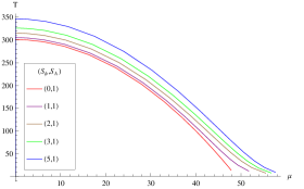
(a)

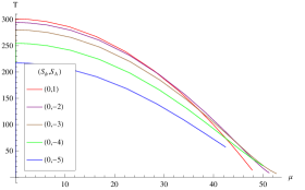
(b)

Figure 3: plot of the phase subspace when $S_{\phi}$ and $S_{A}$ are constant. The red line is the AdS-RN solution.

When the radius of the horizon is fixed, although we have four sources ($T,\mu,S_{\phi},S_{A}$) in the model, the phase space is a three dimensional hypersurface. It is similar to equation (2.11), where temperature and chemical potential are constrained and the phase space is one dimensional. In this case we expect the constraint to be:

$$\frac{\epsilon+P}{s}=T+\mu\;\frac{\rho}{s}+S_{\phi}\;\frac{\langle o\rangle}{s}+S_{A}\;\frac{\langle v\rangle}{s}.$$ (4.17)

In figure (3) we have plotted some curves related to some numerical solutions in the ($T,\mu$) plane, for fixed values of $S_{\phi}$ and $S_{A}$.

From the numerical calculations the following emerges:

1. The solutions with the desired boundary conditions exist only for a limited range of $S_{\phi}$ and $S_{A}$ and also temperature (chemical potential).

2. As is shown in figures (4,5), the vacuum expectation value of the vector operator generally has different signs in different regions of the phase space, and there is a two dimensional surface on which the vacuum expectation value is zero. The sign changes smoothly. This phenomenon can be interpreted as a vortex reversing.

3. At $\mu=S_{\phi}=0$, the sign of $\langle V\rangle$ changes at $(S_{A})_{cr}=0$, or alternatively, $(\tilde{K}_{0})_{cr}=1$. Since the radial nonabelian magnetic field is proportional to $\vec{B}_{r}\propto(1-K(r)^{2})\hat{r}$, the boundary magnetic field is $(\vec{B}_{r})_{boundary}\propto(1-\tilde{K}_{0}^{2})\hat{r}$. So at $\mu=S_{\phi}=0$, the vortex reverses when the boundary magnetic field is reversed.

4. As is clear from figures (4,5), at nonzero chemical potential, even when the boundary magnetic field is zero, the vacuum expectation value of the vector operator can be nonzero; So the vortex can be a condensate. In order to cancel the vortex, we should impose a boundary magnetic field. Increasing $\mu$, increases $(\tilde{K}_{0})_{cr}$ and alternatively $(\vec{B}_{r})_{boundary}$ which is needed to cancel the vortex;and increasing $S_{\phi}$, decreases $(\tilde{K}_{0})_{cr}$.

5. When $S_{\phi}$ is small enough, similar to the vector operator, the vacuum expectation value of the scalar operator has different signs in different regions of the phase space, and there is a two dimensional surface on which the vacuum expectation value is zero, but this time it occurs at low temperatures. This phenomenon can be related to an instability, because in[6], it is shown that such an event occurs for linear fluctuations which means that at some special value of parameters the equations admit a zero mode solution, as a marginal stable mode. For vector fluctuations this is not the case.

(a)

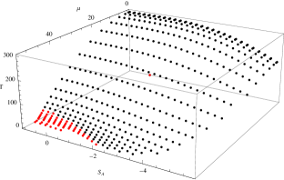
(b)

Figure 4: plot of the phase subspace when $S_{\phi}=0.1$. The red region is where the v.e.vs are negative, and in black region they are positive. Plot (a) is for $\langle V\rangle$, and plot (b) is for $\langle O\rangle$

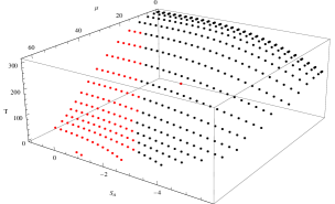
(a)

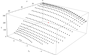
(b)

Figure 5: plot of the phase subspace when $S_{\phi}=1.5$. Plot (a) is for $\langle V\rangle$, and plot (b) is for $\langle O\rangle$. The negative region for $\langle O\rangle$ is disappeared.

5 Conclusion

In this article we studied the vacuum expectation values of dual operators from Einstein-Yang-Mills-Higgs action in a holographic setup and found that the radial magnetic field which is the main property of the magnetic monopoles does not play explicit role in the vacuum expectation values. In particular we consider the Julia-Zee dyon, and saw that the v.e.v of dual scalar and vector operators can be nonzero, and the profile of the vector condensate is similar to a vortex. We also constructed a numerical self-gravitating dyon and studied the changing of the v.e.vs as a function of the sources. We observed a sign changing phenomenon in the v.e.vs by changing temperature, chemical potential, and scalar and vector sources. It will be interesting to check whether these sign changings relate to an instability. Also it seems reasonable to expect that the multi monopole solutions which are studied in[9], correspond to multi vortex configurations in the dual field theory side. Any firm statement on this requires knowledge of the profile of the vector field in the bulk.


Acknowledgements
I would like to thank Farhad Ardalan, for extensive discussions and reading the manuscript, M. Alishahiha and A.E. Mosaffa and also R. Fareghbal, A. Davody, A. Naseh and R. Mozaffari for useful discussions.

References

[1]
J. M. Maldacena,
“The large N limit of superconformal field theories and supergravity,”
Adv. Theor. Math. Phys. 2, 231 (1998)
[Int. J. Theor. Phys. 38, 1113 (1999)]
[arXiv:hep-th/9711200].
[2]
E. Witten,
“Anti-de Sitter space and holography,”
Adv. Theor. Math. Phys. 2, 253 (1998)
[arXiv:hep-th/9802150].
[3]
S. S. Gubser, I. R. Klebanov and A. M. Polyakov,
“Gauge theory correlators from non-critical string theory,”
Phys. Lett. B 428, 105 (1998)
[arXiv:hep-th/9802109].
[4]
A. R. Lugo, E. F. Moreno and F. A. Schaposnik,
“Holographic phase transition from dyons in an AdS black hole background,”
JHEP 1003, 013 (2010)
[arXiv:1001.3378 [hep-th]].
[5]
A. R. Lugo, E. F. Moreno, F. A. Schaposnik,
“Holography and self-gravitating dyons,”
JHEP 1011, 081 (2010).
[arXiv:1007.1482 [hep-th]].
[6]
D. Allahbakhshi, F. Ardalan,
“Holographic Phase Transition to Topological dyons,”
JHEP 1010, 114 (2010).
[arXiv:1007.4451 [hep-th]].
[7]
J. J. van der Bij, E. Radu,
“Magnetic charge, angular momentum and negative cosmological constant,”
Int. J. Mod. Phys. A18, 2379-2393 (2003).
[hep-th/0210185].
[8]
E. Radu, D. H. Tchrakian,
“New axially symmetric Yang-Mills-Higgs solutions with negative cosmological constant,”
Phys. Rev. D71, 064002 (2005).
[hep-th/0411084].
[9]
S. Bolognesi, D. Tong,
“Monopoles and Holography,”
JHEP 1101, 153 (2011).
[arXiv:1010.4178 [hep-th]].
[10]
P. Sutcliffe,
“Monopoles in AdS,”. [arXiv:1104.1888 [hep-th]].
[11]
M. Kasuya and M. Kamata,
“An Exact Dyon Solution With The Reissner-Nordstrom Metric,”
Nuovo Cim. B 66, 75 (1981).
[12]
J. Arafune, P. G. O. Freund and C. J. Goebel,
“Topology Of Higgs Fields,”
IN *Kyoto 1975, Proceedings. Lecture Notes in Physics*,
Berlin 1975, 240-241