The two-loop hemisphere soft function

Randall Kelley and Matthew D. Schwartz
Center for the Fundamental Laws of Nature
Harvard University
Cambridge, MA 02138, USA

Robert M. Schabinger

Instituto de Física Teórica UAM/CSIC
Universidad Autónoma de Madrid
Cantoblanco, E-28049 Madrid, España
Hua Xing Zhu
Department of Physics and State Key Laboratory of Nuclear Physics and Technology
Peking University
Beijing 100871, China

The hemisphere soft function is calculated to order $\alpha_{s}^{2}$. This is the first multi-scale soft function calculated to two loops. The renormalization scale dependence of the result agrees exactly with the prediction from effective field theory. This fixes the unknown coefficients of the singular parts of the two-loop thrust and heavy-jet mass distributions. There are four such coefficients, for 2 event shapes and 2 color structures, which are shown to be in excellent agreement with previous numerical extraction. The asymptotic behavior of the soft function has double logs in the $C_{F}C_{A}$ color structure, which agree with non-global log calculations, but also has sub-leading single logs for both the $C_{F}C_{A}$ and $C_{F}T_{F}n_{f}$ color structures. The general form of the soft function is complicated, does not factorize in a simple way, and disagrees with the Hoang-Kluth ansatz. The exact hemisphere soft function will remove one source of uncertainty on the $\alpha_{s}$ fits from $e^{+}e^{-}$ event shapes.

1 Introduction

There has been significant activity in the last few years in the effective field community to perform accurate calculations of event shapes for $e^{+}e^{-}$ colliders. At high energy, the hadronic final states in $e^{+}e^{-}$ collisions are dominated by the formation of jets of particles and are described by perturbative QCD. Comparison of theoretic calculations of event shapes with the experimentally measured values has lead to some of the most precise measurements of the strong coupling constant $\alpha_{s}$. The NNLO fixed order calculations in [1, 2, 3, 4] allow the prediction of many events shapes to order $\alpha_{s}^{3}$. Advances in Soft-Collinear Effective Theory (SCET) [5, 6, 7, 8] have allowed for resummation of large logarithmic corrections to thrust [9, 10, 11] and heavy jet mass [12] to ${\rm N^{3}LL}$ accuracy and non-perturbative considerations were included for thrust in [13]. These results have been used to extract a value of $\alpha_{s}$ that is competitive with the world average [14].

Dijet event shapes such as thrust and heavy jet mass demonstrate singular behavior when calculated perturbatively at fixed order due to the appearance of large logarithmic corrections. These large logarithms invalidate a naive expansion in $\alpha_{s}$ and thus need to be resummed to provide accurate predictions in the dijet limit. In the dijet limit, there is a clear separation between scales. Effective theory techniques rely on a separation between kinematic scales and, through renormalization group (RG) evolution, logarithms of the ratio of these scales can be resummed. Each of the relevant scales is described by different physics, each of which can be calculated using a different theory. The contribution from each can be shown to factorize into a hard contribution, due to physics at the center of mass energy $Q$, a jet function, due to physics at the jet scale, and a soft function which describes soft gluon emission. The hard and jet functions are known to 2-loops. However, the soft function relevant for thrust or heavy jet mass is only partially known beyond 1-loop [15, 12]. In this paper, the perturbative soft function is computed analytically to order $\alpha_{s}^{2}$.

Soft functions have been studied for many years, not just in SCET. These soft functions are defined as matrix elements of Wilson lines. For resummation up to the next-to-leading logarithmic order (NLL), all that is needed about the soft function is its anomalous dimension. This can be extracted either from renormalization-group invariance or from the virtual graphs. For example, such calculations have been done for thrust [11], direct photon [16], and dijet production [17, 18, 20, 21]. To go beyond NLL, one needs the finite parts of these soft functions, which are more difficult to calculate because the real emission graphs are needed, and these involve often complicated phase-space cuts. In all cases calculated at 2-loops so far, such as Drell-Yan [22, 23] or $b\to s\gamma$ [24], the real emission graphs only involve one scale. Multi-scale soft functions, where different constraints are placed on gluons or quarks going in different directions, such as the hemisphere soft function, are likely to play an important role in hadron collisions [19, 25]. At order $\alpha_{s}$, the multiple scales are irrelevant, since only one gluon can be emitted. At order $\alpha_{s}^{2}$ or beyond, there can be real emission graphs depending on multiple scales at the same time. It has been suggested [15] that the soft function should depend only on logarithms of these scales, such as $\ln^{2}(k_{L}/k_{R})$. Whether more complicated scale-independent terms, such as $\text{Li}_{2}(-{k_{L}/k_{R}})+\text{Li}_{2}(-{k_{R}/k_{L}})$ might appear has been an open question. Understanding the form of these soft functions in more detail will be important for LHC precision jet physics at NNLL and beyond [25].

The hemisphere soft function $S(k_{L},k_{R},\mu)$ is the probability to have soft radiation with small component $k_{L}$ going into the left hemisphere and soft radiation with small component $k_{R}$ going into the right hemisphere. More precisely, in $e^{+}e^{-}\to$ hadron events at center-of-mass energy $Q$, in the limit that all radiation is much softer than $Q$, the cross section is given by matrix elements of Wilson lines. These Wilson lines point in the direction of two back-to-back light-like quarks which come from the Born process $e^{+}e^{-}\to\bar{q}q$. Each quark direction defines a hemisphere, which we call left and right and denote with the light-like 4-vectors $n^{\mu}$ and $\bar{n}^{\mu}$. If the total radiation in the left (right) hemisphere is $P_{L}^{\mu}$ ($P_{R}^{\mu}$), then $S(k_{L},k_{R},\mu)$ is the matrix element squared to have $k_{L}=n\cdot P_{L}$ and $k_{R}=\bar{n}\cdot P_{R}$, with all other degrees of freedom integrated over.

The hemisphere soft function is known to have many interesting properties and is conjectured to have others. The factorization theorem for the full hemisphere mass distribution implies that the Laplace transform of the soft function should factorize into the form

$$\tilde{s}(L_{1},L_{2},\mu)=\widetilde{s}_{\mu}(L_{1})\widetilde{s}_{\mu}(L_{2})\widetilde{s}_{f}(L_{1}-L_{2})$$ (1)

where $L_{1}=\ln x_{L}\mu$ and $L_{2}=\ln x_{R}\mu$, with $x_{R}$ and $x_{L}$ the Laplace conjugate variables to $k_{L}$ and $k_{R}$. The anomalous dimension of the soft function and the function $\tilde{s}_{\mu}(L)$ are known exactly to 3-loop order. The function $\tilde{s}_{f}(L)$ is known exactly only to order $\alpha_{s}$. Hoang and Kluth [15] argued that at order $\alpha_{s}^{2}$ the function $\tilde{s}_{f}(L)$ must be a polynomial of at most 2nd order in $L$, i.e. $\widetilde{s}_{f}(L)=c_{2}^{S}+c_{2L}^{S}L^{2}$. In this paper, we show that this Hoang-Kluth ansatz does not hold; $\widetilde{s}_{f}(L)$ is much more complicated. Certain moments of $\widetilde{s}_{f}(L)$ contribute to the coefficients of $\delta(\tau)$ and $\delta(\rho)$ in the thrust and heavy-jet mass distributions. These moments were fit numerically in [15] and [12] using numerical calculations of the singular behaviour of these distributions in full QCD with the program event 2. In this paper, we produce these moments analytically and find that they are in excellent agreement with the most accurate available numerical fit [12].

Any $L$ dependence at large $L$ in $\widetilde{s}_{f}(L)$ turns into large logarithmic behavior of the hemisphere mass distribution (i.e. $\ln(M_{L}/M_{R}$)). Since all of the $\mu$ dependence is in $\widetilde{s}_{\mu}(L)$, these large logs are not determined by RG invariance and correspond to so-called “non-global logs”. Dasgupta and Salam calculated the non-global logs for the related left-hemisphere mass distribution in full QCD [26] and found no non-global logs (up to order $L^{2}$) for the $C_{F}n_{f}T_{F}$ color structure and an $L^{2}$ term with coefficient $-\frac{4\pi^{2}}{3}$ for the $C_{F}C_{A}$ term. We show below that the asymptotic behavior of $\widetilde{s}_{f}(L)$ in the full soft function is indeed of the form $-\frac{4\pi^{2}}{3}L^{2}$ for the $C_{F}C_{A}$ color structure. We also find that both this color structure and the $C_{F}n_{f}T_{F}$ one have additional non-global single logs. These are especially interesting because the soft function is symmetric in $L\to-L$, which seems to forbid a linear term. The linear term appears through a complicated analytic function involving polylogarithms which actually asymptotes to $|L|$.

This paper is organized as follows. In section 2 we review the factorization formula for the hemisphere mass distribution and its thrust and heavy-jet mass projections. Section 3 computes the soft function in dimensional regularization. The calculation is complicated, so the results are summarized separately in 3.3. Section 4 discusses the result and presents the renormalized result for the integrated soft function, which can be compared directly to the predictions from SCET. Section  5 gives the previously missing terms in the singular parts of the 2-loop thrust and heavy jet mass distributions, and compares to previous numerical estimates. Section 6 gives the full integrated hemisphere soft function which is compared to previous conjectures. The asymptotic form of this distribution, which exhibits non-global logs, is discussed in Section 7. Section 8 has some comments on predicting higher order terms with non-Abelian exponentiation. Conclusions and implications are discussed in Section 9.

2 Event Shapes and Factorization in SCET

The hemisphere soft function appears in the factorization theorem for the hemisphere mass distribution. The hemispheres are defined with respect to the thrust axis. Thrust itself is defined by

$$T=\max_{\mathbf{n}}\left(\frac{\sum_{i}|{\mathbf{p}}_{i}\cdot{\mathbf{n}}|}{\sum_{i}|\mathbf{p}_{i}|}\right),$$ (2)

where the sum is over all momentum 3-vectors $\mathbf{p}_{i}$ in the event. The thrust axis is the unit 3-vector $\mathbf{n}$ that maximizes the expression in parentheses. We then define the light-like 4-vectors $n^{\mu}=(1,\mathbf{n})$ and $\bar{n}^{\mu}=(1,-\mathbf{n})$. In the dijet limit $T\to 1$ and it is therefore more convenient to define $\tau=1-T$ as the thrust variable so that $\tau$ is small in the dijet limit.

Once the thrust axis is known, we divide the event into two hemispheres defined by the plane perpendicular to the thrust axis. We define $P_{L}^{\mu}$ and $P_{R}^{\mu}$ to be the 4-vector sum of all of the radiation going into each hemisphere and $M_{L}=\sqrt{P_{L}^{2}}$ and $M_{R}=\sqrt{P_{R}^{2}}$ to be the hemisphere invariant masses. When both $M_{L}$ and $M_{R}$ are small compared to the center-of-mass energy, $Q$, the hemisphere mass distribution factorizes into [8]

$$\frac{1}{\sigma_{0}}\frac{\mathrm{d}^{2}\sigma}{\mathrm{d}M_{L}^{2}\mathrm{d}M_{R}^{2}}=H(Q^{2},\mu)\int\mathrm{d}k_{L}\mathrm{d}k_{R}J(M_{L}^{2}-Qk_{L},\mu)J(M_{R}^{2}-Qk_{R},\mu)S(k_{L},k_{R},\mu)\,.$$ (3)

Here, $\sigma_{0}$ is the tree level total cross section. $H(Q^{2},\mu)$ is the hard function which accounts for the matching between QCD and SCET. $J(p^{2})$ is the inclusive jet function which accounts for the matching between an effective field theory with soft and collinear modes to a theory with only soft modes. Finally, the object of interest, $S(k_{L},k_{R},\mu)$ is the hemisphere soft function, which is derived by integrating out the remaining soft modes.

In the threshold limit (small hemisphere masses), the thrust axis aligns with the jet axis and thrust can be written as the sum of the two hemisphere masses,

$$\tau=\frac{M_{L}^{2}+M_{R}^{2}}{Q^{2}}+\mathcal{O}\left(\frac{M_{L,R}^{4}}{Q^{4}}\right)$$ (4)

Heavy jet mass $\rho$ is defined to be the larger of the two hemisphere masses, normalized to the center of mass energy $Q$,

$$\rho=\frac{1}{Q^{2}}\max(M_{L}^{2},M_{R}^{2}).$$ (5)

When $\rho$ is small, both hemisphere masses are small and the event appears as two pencil-like, back to back jets.

The factorization formula can be used to calculate thrust and heavy jet mass in the dijet limit as integrals over the doubly differential hemisphere mass distribution. Explicitly,

$$\frac{\mathrm{d}\sigma}{\mathrm{d}\tau}=Q^{2}\int\mathrm{d}M_{L}^{2}\mathrm{d}M_{R}^{2}\frac{\mathrm{d}^{2}\sigma}{\mathrm{d}M_{L}^{2}\mathrm{d}M_{R}^{2}}\delta(Q^{2}\tau-M_{L}^{2}-M_{R}^{2})$$ (6)

and

$$\frac{\mathrm{d}\sigma}{\mathrm{d}\rho}=Q^{2}\int\mathrm{d}M_{L}^{2}\mathrm{d}M_{R}^{2}\frac{\mathrm{d}^{2}\sigma}{\mathrm{d}M_{L}^{2}\mathrm{d}M_{R}^{2}}\left[\delta(Q^{2}\rho-M_{L}^{2})\theta(M_{L}^{2}-M_{R}^{2})+\delta(Q^{2}\rho-M_{R}^{2})\theta(M_{R}^{2}-M_{L}^{2})\right]\,.$$ (7)

The thrust distribution can be written so that it depends not on the full hemisphere soft function but on the thrust-soft function, defined as

$$S_{T}(k,\mu)=\int\mathrm{d}k_{L}\mathrm{d}k_{R}S(k_{L},k_{R},\mu)\delta(k-k_{L}-k_{R})\,.$$ (8)

Since the thrust soft function is dimensionless and its $\mu$ dependence is determined by renormalization group invariance, the $k$ dependence is also completely known. Thus at each order in $\alpha_{s}$ only one number, the constant part, is unknown. In contrast, for the heavy jet mass distribution, the full $k_{L}$ and $k_{R}$ dependence of the soft function is needed for the factorization theorem. In particular, for resummation to N³LL order, only one number is needed for thrust (the constant in the 2-loop thrust soft function), which has been fit numerically, but for heavy-jet mass a function is needed [12]. In this paper we compute both the number and the function.

3 Calculation of the Soft Function

The soft function is defined as

$$S(k_{L},k_{R},\mu)\equiv\frac{1}{N_{c}}\sum_{X_{s}}\delta(k_{R}-n\cdot P_{s}^{R})\delta(k_{L}-{\bar{n}}\cdot P_{s}^{L})\left<0\right|\overline{Y}_{{\bar{n}}}Y_{n}\left|X_{s}\right>\left<X_{s}\right|Y^{\dagger}_{n}\overline{Y}^{\dagger}_{{\bar{n}}}\left|0\right>,$$ (9)

where $P_{s}^{L,R}$ is the total momentum of the final state $\left|X_{s}\right>$ in the left and right hemisphere, respectively. The Wilson lines $Y_{n}$ and $\overline{Y}_{{\bar{n}}}$ are defined by

$$Y^{\dagger}_{n}(x)=P\exp\left(ig\int_{0}^{\infty}\!\!ds\ n\cdot A_{s}(ns+x)\right) \overline{Y}^{\dagger}_{{\bar{n}}}(x)=P\exp\left(ig\int_{0}^{\infty}\!\!ds\ {\bar{n}}\cdot\overline{A}_{s}(ns+x)\right),$$ (10)

where $P$ denotes path ordering and $A_{s}=A^{a}_{s}T^{a}$ $(\overline{A}_{s}=A_{s}^{a}\overline{T}^{a})$ are gauge fields in the fundamental (anti-fundamental) representation. The soft function can be factorized into a perturbative (partonic) part and non-perturbative part which has support of order $\Lambda_{QCD}$ [13].

The authors of [15] observed that the form of the soft function is constrained by the non-Abelian exponentiation theorem and RG invariance, which puts constraints on powers of logarithms of $\mu$. The theorem also restricts the $C_{F}^{n}$ color structure in the soft function to be completely determined by the one-loop result. Beyond this, however, the soft function is unconstrained. The one-loop calculation was done in [9, 27]. The main result of this paper is the calculation of the perturbative part of the hemisphere soft function to order $\alpha_{s}^{2}$. Since the order $\alpha_{s}^{2}$ color structure $C_{F}^{2}$ is given in [15], we will only calculate the $C_{F}C_{A}$ and the $C_{F}n_{f}T_{F}$ terms.

3.1 $C_{F}C_{A}$ color structure

The order $\alpha_{s}^{2}$ calculation involves pure virtual graphs, pure real emission graphs, and interference between the two. The pure virtual contributions to the soft function give scaleless integrals which convert IR divergences to UV divergences, and are not explicitly written. The diagrams needed to compute the pure real emission contributions are shown in Figs. 1-4, whereas the interference graphs between the order $\alpha_{s}$ real and virtual emission amplitudes are shown in Fig. 5.

The integrals corresponding to the two diagrams in Fig. 1 (and the twin of diagram A obtained by interchanging $k$ and $q$) are given, in $d=4-2\epsilon$ dimensions using the $\overline{\text{MS}}$ scheme, by

$$I_{{\color[rgb]{0.0,0.0,0.9}A}}=2(-4g^{4})\left(C_{F}^{2}-\frac{C_{F}C_{A}}{2}\right)\left(\frac{\mu^{2}e^{\gamma_{E}}}{4\pi}\right)^{2\epsilon}\int\frac{\mathrm{d}^{d}q}{(2\pi)^{d}}\int\frac{\mathrm{d}^{d}k}{(2\pi)^{d}}\frac{1}{k^{-}k^{+}q^{-}q^{+}}F(k_{L},k_{R})$$ (11)

and

$$I_{{\color[rgb]{0.0,0.0,0.9}B}}=-4g^{4}\left(\frac{\mu^{2}e^{\gamma_{E}}}{4\pi}\right)^{2\epsilon}\int\frac{\mathrm{d}^{d}q}{(2\pi)^{d}}\int\frac{\mathrm{d}^{d}k}{(2\pi)^{d}}\frac{1}{(k^{+}+q^{+})(k^{-}+q^{-})}$$

$$\qquad\times\left\{\left(C_{F}^{2}-\frac{C_{F}C_{A}}{2}\right)\left(\frac{1}{k^{-}k^{+}}+\frac{1}{q^{-}q^{+}}\right)+C_{F}^{2}\left(\frac{1}{k^{-}q^{+}}+\frac{1}{q^{-}k^{+}}\right)\right\}F(k_{L},k_{R}),$$ (12)

where $k^{-}={\bar{n}}\cdot k$, $k^{+}=n\cdot k$ and $F(k_{L},k_{R})$ contains the $\delta(q^{2})$ and $\delta(k^{2})$ factors which put the emitted gluons on shell and the phase-space restrictions in the definition of the hemisphere soft function. Explicitly, $F(k_{L},k_{R})$ is given by

$$F(k_{L},k_{R}) =\frac{1}{2!}(-2\pi i)^{2}\delta(k^{2})\delta(q^{2})$$

$$\times\Bigl{[}\Theta(k^{-}-k^{+})\Theta(q^{+}-q^{-})\delta(k^{+}-k_{R})\delta(q^{-}-k_{L})$$

$$\ \ +\Theta(k^{+}-k^{-})\Theta(q^{-}-q^{+})\delta(k^{-}-k_{L})\delta(q^{+}-k_{R})$$

$$\ \ +\Theta(k^{-}-k^{+})\Theta(q^{-}-q^{+})\delta(k^{+}+q^{+}-k_{R})\delta(k_{L})$$

$$\ \ +\Theta(q^{+}-q^{-})\Theta(k^{+}-k^{-})\delta(k^{-}+q^{-}-k_{L})\delta(k_{R})\Bigr{]}.$$ (13)

In each diagram, the momentum has been routed so that the 4-vectors $k$ and $q$ correspond to the final state gluons. The gluonic contribution to the $C_{F}C_{A}$ color factor will be symmetric in $k$ and $q$ due to the fact that the radiated gluons are identical particles. In the first diagram, a factor of two has been added since the integrand is unchanged after $k\leftrightarrow q$, whereas in the second diagram, the SCET Feynman rules for two gluon emission from a single soft Wilson line automatically account for $k\leftrightarrow q$. The factor of $1/2!$ needed for averaging over $k\leftrightarrow q$ is in $F(k_{L},k_{R})$. Not shown in Fig. 1 is the graph that corresponds to the complex conjugate of diagram B. This diagram gives the same integral as diagram B. Since we are interested in the $C_{F}C_{A}$ contribution, the linear combination of interest is $I_{{\color[rgb]{0.0,0.0,0.9}A}}+2I_{{\color[rgb]{0.0,0.0,0.9}B}}$. Diagram A and its identical twin are self-conjugate and only contribute once because they represent the squares of tree-level Feynman diagrams.

Figure 1: Diagrams A and B contribute to both $C_{F}^{2}$ and $C_{F}C_{A}$ color factors.

Figure 2: Diagrams C and D contribute to the $C_{F}C_{A}$ color factor.

Figure 3: Diagrams E and F contribute to the $C_{F}C_{A}$ color factor.

Figure 4: Diagrams G, H and I. These classes of diagrams contribute to integrals $I_{{\color[rgb]{0.0,0.0,0.9}G}},I_{{\color[rgb]{0.0,0.0,0.9}H}}$, and $I_{{\color[rgb]{0.0,0.0,0.9}I}}$ when the self-energy graphs involve gluons or ghosts and they contribute to integrals $\tilde{I}_{{\color[rgb]{0.0,0.0,0.9}G}},\tilde{I}_{{\color[rgb]{0.0,0.0,0.9}H}}$, and $\tilde{I}_{{\color[rgb]{0.0,0.0,0.9}I}}$ when the self-energy graphs involve a fermion/anti-fermion pair.

Figure 5: Diagrams J and K account for the interference between the one-loop virtual emission amplitude and the single gluon emission amplitude. Diagram L is the contribution from charge renormalization.

There are four classes of diagrams involving the triple gauge coupling. Diagrams C and D, shown in Fig. 2, give the following integrals,

$$I_{{\color[rgb]{0.0,0.0,0.9}C}} =-g^{4}C_{A}C_{F}\left(\frac{\mu^{2}e^{\gamma_{E}}}{4\pi}\right)^{2\epsilon}\int\frac{\mathrm{d}^{d}q}{(2\pi)^{d}}\int\frac{\mathrm{d}^{d}k}{(2\pi)^{d}}\frac{F(k_{L},k_{R})}{(k^{-}+q^{-})(k+q)^{2}}\left(\frac{k^{-}+2q^{-}}{k^{+}q^{-}}+\frac{q^{-}+2k^{-}}{q^{+}k^{-}}\right)$$ (14)

$$I_{{\color[rgb]{0.0,0.0,0.9}D}} =-g^{4}C_{A}C_{F}\left(\frac{\mu^{2}e^{\gamma_{E}}}{4\pi}\right)^{2\epsilon}\int\frac{\mathrm{d}^{d}q}{(2\pi)^{d}}\int\frac{\mathrm{d}^{d}k}{(2\pi)^{d}}\frac{F(k_{L},k_{R})}{(k^{+}+q^{+})(k+q)^{2}}\left(\frac{2k^{+}+q^{+}}{k^{+}q^{-}}+\frac{2q^{+}+k^{+}}{q^{+}k^{-}}\right)$$ (15)

whereas, diagrams E and F, shown in Fig 3, give

$$I_{{\color[rgb]{0.0,0.0,0.9}E}}=g^{4}C_{F}C_{A}\left(\frac{\mu^{2}e^{\gamma_{E}}}{4\pi}\right)^{2\epsilon}\int\frac{\mathrm{d}^{d}q}{(2\pi)^{d}}\int\frac{\mathrm{d}^{d}k}{(2\pi)^{d}}\\ \qquad\times\left(\frac{1}{q^{-}}-\frac{1}{k^{-}}\right)\frac{q^{-}-k^{-}}{(k^{+}+q^{+})(k^{-}+q^{-})(k+q)^{2}}F(k_{L},k_{R})$$ (16)

$$I_{{\color[rgb]{0.0,0.0,0.9}F}}=g^{4}C_{F}C_{A}\left(\frac{\mu^{2}e^{\gamma_{E}}}{4\pi}\right)^{2\epsilon}\int\frac{\mathrm{d}^{d}q}{(2\pi)^{d}}\int\frac{\mathrm{d}^{d}k}{(2\pi)^{d}}\\ \qquad\times\left(\frac{1}{k^{+}}-\frac{1}{q^{+}}\right)\frac{k^{+}-q^{+}}{(k^{+}+q^{+})(k^{-}+q^{-})(k+q)^{2}}F(k_{L},k_{R})$$ (17)

Each of these diagrams has a complex conjugate and so they contribute twice.

There are three self-energy topologies, shown in Fig. 4. The gluon and ghost self-energy graphs contribute to integrals $I_{{\color[rgb]{0.0,0.0,0.9}G}},I_{{\color[rgb]{0.0,0.0,0.9}H}}$ and $I_{{\color[rgb]{0.0,0.0,0.9}I}}$ below.

$$I_{{\color[rgb]{0.0,0.0,0.9}G}}=g^{4}C_{F}C_{A}\left(\frac{\mu^{2}e^{\gamma_{E}}}{4\pi}\right)^{2\epsilon}\int\frac{\mathrm{d}^{d}q}{(2\pi)^{d}}\int\frac{\mathrm{d}^{d}k}{(2\pi)^{d}}\frac{1}{(k^{-}+q^{-})(k^{+}+q^{+})(k+q)^{4}}\\ \qquad\times\Bigl{[}q^{+}[(d-6)q^{-}-(d+2)k^{-}]+k^{+}[(d-6)k^{-}-(d+2)q^{-}]+16k\cdot q\Bigr{]}F(k_{L},k_{R})$$ (18)

$$I_{{\color[rgb]{0.0,0.0,0.9}H}}=g^{4}C_{F}C_{A}\left(\frac{\mu^{2}e^{\gamma_{E}}}{4\pi}\right)^{2\epsilon}\int\frac{\mathrm{d}^{d}q}{(2\pi)^{d}}\int\frac{\mathrm{d}^{d}k}{(2\pi)^{d}}\frac{1}{(k^{-}+q^{-})^{2}(k+q)^{4}}\\ \qquad\times\Bigl{[}2(d+2)q^{-}k^{-}-(d-6)(k^{-})^{2}-(d-6)(q^{-})^{2}\Bigr{]}F(k_{L},k_{R})$$ (19)

$$I_{{\color[rgb]{0.0,0.0,0.9}I}}=g^{4}C_{F}C_{A}\left(\frac{\mu^{2}e^{\gamma_{E}}}{4\pi}\right)^{2\epsilon}\int\frac{\mathrm{d}^{d}q}{(2\pi)^{d}}\int\frac{\mathrm{d}^{d}k}{(2\pi)^{d}}\frac{1}{(k^{+}+q^{+})^{2}(k+q)^{4}}\\ \qquad\times\Bigl{[}2(d+2)q^{+}k^{+}-(d-6)(k^{+})^{2}-(d-6)(q^{+})^{2}\Bigr{]}F(k_{L},k_{R})$$ (20)

As usual, cutting Feynman diagrams removes any symmetry factors that were associated to the cut lines prior to cutting. It is also worth reminding the reader that, in order to consistently combine the ghost emission diagrams with the gluon emission diagrams, we have to double-count the ghosts (they do not have the $1/2!$ symmetry factor that the gluons do). Diagram G has a complex conjugate graph which must be included but diagrams H and I, like diagram A, represent squares of tree-level Feynman diagrams and are therefore self-conjugate.

Adding all of these contributions together, we have

$$S^{R}_{C_{A}}(k_{L},k_{R})=I_{{\color[rgb]{0.0,0.0,0.9}A}}+I_{{\color[rgb]{0.0,0.0,0.9}H}}+I_{{\color[rgb]{0.0,0.0,0.9}I}}+2(I_{{\color[rgb]{0.0,0.0,0.9}B}}+I_{{\color[rgb]{0.0,0.0,0.9}C}}+I_{{\color[rgb]{0.0,0.0,0.9}D}}+I_{{\color[rgb]{0.0,0.0,0.9}E}}+I_{{\color[rgb]{0.0,0.0,0.9}F}}+I_{{\color[rgb]{0.0,0.0,0.9}G}})\qquad(\text{$C_{F}C_{A}$ part})$$

$$\qquad=g^{4}C_{F}C_{A}\left(\frac{\mu^{2}e^{\gamma_{E}}}{4\pi}\right)^{2\epsilon}\int\frac{\mathrm{d}^{d}q}{(2\pi)^{d}}\int\frac{\mathrm{d}^{d}k}{(2\pi)^{d}}\Bigl{\{}\frac{2}{(k\cdot q)^{2}k^{-}k^{+}q^{-}q^{+}(k^{-}+q^{-})(k^{+}+q^{+})}$$

$$\qquad\times\Bigl{[}-k\cdot q\Bigl{(}(k^{-})^{2}q^{+}(2k^{+}+q^{+})+2k^{-}q^{-}\left((k^{+})^{2}-k^{+}q^{+}+(q^{+})^{2}\right)+k^{+}(q^{-})^{2}(k^{+}+2q^{+})\Bigr{)}$$

$$\qquad+2(k\cdot q)^{2}\Bigl{(}k^{-}(2k^{+}+q^{+})+q^{-}(k^{+}+2q^{+})\Bigr{)}\Bigr{]}$$

$$\qquad+(\epsilon-1)\frac{2(k^{+}q^{-}-k^{-}q^{+})^{2}}{(k\cdot q)^{2}(k^{-}+q^{-})^{2}(k^{+}+q^{+})^{2}}\Bigr{\}}F(k_{L},k_{R})\,.$$ (21)

Before presenting the result for the $C_{F}C_{A}$ color factor, we briefly describe our general computational strategy. Normally, one expects scaleless integrals to be simpler than single scale integrals. In this particular case, the single scale integrals (with scale $k_{L}/k_{R}$) are actually much less technically demanding. This is true primarily because these contributions (see the first two terms of Eq. (3.1)) are integrable at $\epsilon=0$. It turns out that this special feature of the problem more than makes up for the fact that single scale integrals are generically harder to evaluate than scaleless integrals.

The calculation proceeds as follows for a single scale integral. First there will be an integral over angles (the integrand depends non-trivially on $k\cdot q$) that can be done analytically to all orders in $\epsilon$. It is then convenient to Taylor series expand the resulting hypergeometric functions using the HypExp package [28] for Mathematica. In fact, the whole integrand can be expanded in a Taylor series in $\epsilon$ and integrated term-by-term, due to the fact that the integral converges at $\epsilon=0$. With a modest amount of knowledge of the basic functional identities satisfied by the polylogarithm functions, it is possible to do the resulting two-fold one-parameter integral in Mathematica and express the final result in terms of a minimal basis of transcendental functions. The results of our single scale calculations for both non-trivial color factors are tabulated in the Appendix.

The evaluation of a scaleless integral (originating from the last two terms of Eq. (3.1)) begins in much the same way. Unfortunately, it quickly becomes clear that what remains after integrating over all angles has a non-trivial analytical structure (considered as a function of $\epsilon$). In particular, the integral diverges at $\epsilon=0$. Expanding an integral of this class under the integral sign is significantly more complicated and requires new tools. To begin, one should transform all hypergeometric functions in the integrand and expose their singularity structure. In this fashion, one learns that there is a line of singularities within the region of integration. A well-known procedure called sector decomposition [29] allows one to move singularities within the region of integration to singularities on the boundaries of the region of integration. Sector decomposition works as follows. Through a sequence of variable changes and interchanges of integration orders, all phase-space singularities are put into a canonical form. At this point, one can use an expansion in distributions to extract singularities in $\epsilon$ under the integral sign. Finally, the entire integrand can be expanded in $\epsilon$ in terms of distributions and ordinary functions and one can integrate the Laurent series term-by-term.

Once we understood the computational procedure described above, it was straightforward to evaluate the integrals of interest for the $C_{F}C_{A}$ color factor. The result has the form

$$S^{R}_{C_{A}}(k_{L},k_{R})=\left(\frac{\alpha}{4\pi}\right)^{2}C_{F}C_{A}\left[\frac{\mu^{4\epsilon}}{(k_{R}k_{L})^{1+2\epsilon}}f_{C_{A}}\left(\frac{k_{L}}{k_{R}},\epsilon\right)+\left(\frac{\mu^{4\epsilon}}{k_{L}^{1+4\epsilon}}\delta(k_{R})+\frac{\mu^{4\epsilon}}{k_{R}^{1+4\epsilon}}\delta(k_{L})\right)g_{C_{A}}(\epsilon)\right].$$

The first term corresponds to the first two terms in Eq. (3.1), those that account for the possibility that exactly one gluon is radiated into each hemisphere. It depends on $f_{C_{A}}(r,\epsilon)$, a dimensionless function of $r=k_{L}/k_{R}$ and $\epsilon$. It can be written as an expansion in $\epsilon$ as

$$f_{C_{A}}(r,\epsilon) =f_{C_{A}}^{(0)}(r)+\epsilon f_{C_{A}}^{(1)}(r)+\epsilon^{2}f_{C_{A}}^{(2)}(r)+\cdots.$$ (22)

The expressions for $f_{C_{A}}^{(n)}(r)$ are quite lengthy and are given in the appendix for $n=0,1,2$. The second term in Eq. (3.1) accounts for the fact that both gluons can propagate into the same hemisphere and it has no non-trivial $k_{L}$ or $k_{R}$ dependence. $g_{C_{A}}(\epsilon)$ is simply a constant with $\epsilon$ expansion

$$g_{C_{A}}(\epsilon) =\frac{4}{\epsilon^{3}}+\frac{22}{3\epsilon^{2}}+\frac{1}{\epsilon}\left(\frac{134}{9}-\frac{4\pi^{2}}{3}\right)-\frac{116\zeta_{3}}{3}+\frac{11\pi^{2}}{9}+\frac{772}{27}$$

$$\qquad+\left(\frac{484\zeta_{3}}{9}+\frac{4784}{81}+\frac{67\pi^{2}}{27}-\frac{137\pi^{4}}{90}\right)\epsilon.$$ (23)

The interference between the one-loop and tree-level single gluon emission amplitudes is shown in diagrams J and K of Fig. 5. The integrals associated with diagram J are scaleless and are set to zero in dimensional regularization. Diagram K gives the integral

$$I_{{\color[rgb]{0.0,0.0,0.9}{\color[rgb]{0.0,0.0,0.9}K}}} =4(-g^{4})C_{A}C_{F}\int\frac{\mathrm{d}^{d}q}{(2\pi)^{d}}\frac{1}{q^{-}}\int\frac{\mathrm{d}^{d}k}{(2\pi)^{d}}\frac{2q^{-}-k^{-}}{k^{+}(q^{-}-k^{-})(q-k)^{2}k^{2}}$$

$$\qquad\times(-2\pi i)\delta(q^{2})[\Theta(q^{-}-q^{+})\delta(q^{+}-k_{R})\delta(k_{L})+\Theta(q^{+}-q^{-})\delta(q^{-}-k_{L})\delta(k_{R})].$$ (24)

There are 2 diagrams with the topology of diagram K. When they are considered with single real emission phase-space cuts, they can easily be mapped into each other and therefore give identical results. Both diagrams also have a complex conjugate graph and these obviously give equal contributions as well. This is why $I_{{\color[rgb]{0.0,0.0,0.9}{\color[rgb]{0.0,0.0,0.9}K}}}$ has an overall factor of 4 out front. After evaluating this integral, the real-virtual interference contribution becomes

$$S^{\rm V}_{C_{A}}(k_{L},k_{R}) =\left(\frac{\alpha}{4\pi}\right)^{2}C_{F}C_{A}\left(\frac{\mu^{4\epsilon}}{k_{L}^{1+4\epsilon}}\delta(k_{R})+\frac{\mu^{4\epsilon}}{k_{R}^{1+4\epsilon}}\delta(k_{L})\right)v_{C_{A}}(\epsilon),$$ (25)

where $v_{C_{A}}(\epsilon)$ can be expanded in $\epsilon$ as

$$v_{C_{A}}(\epsilon) =-\frac{4}{\epsilon^{3}}+\frac{2\pi^{2}}{\epsilon}+\frac{32\zeta_{3}}{3}-\epsilon\frac{\pi^{4}}{30}.$$ (26)

It is worth noting that, in this case, the application of the optical theorem for Feynman diagrams is a bit subtle; one finds an explicit factor of ${\rm exp}(\pm i\pi\epsilon)$ after doing the $k$ integral (the sign of the phase depends on the precise pole prescription). Cutkosky’s rules still apply provided that one keeps only the appropriate projection of the complex phase. After a moment’s thought it becomes clear that the real part, $\cos(\pi\epsilon)$ (independent of the pole prescription), is what one needs to keep to complete the calculation and derive the above result.

The result of diagram L, including the complex conjugate graph, is given by

$$S^{\rm Ren}(k_{L},k_{R}) =-\left(\frac{\alpha}{4\pi}\right)^{2}C_{F}\left(\frac{\mu^{2\epsilon}}{k_{L}^{1+2\epsilon}}\delta(k_{R})+\frac{\mu^{2\epsilon}}{k_{R}^{1+2\epsilon}}\delta(k_{L})\right)\frac{4e^{\gamma_{E}}}{\epsilon^{2}\Gamma(1-\epsilon)}\beta_{0}$$ (27)

where $\beta_{0}=\frac{11}{3}C_{A}-\frac{4}{3}n_{f}T_{F}$ is the first expansion coefficient of the QCD $\beta$-function, $\beta(g)/g=\frac{\alpha_{s}}{4\pi}\beta_{0}$. Finally, the total contribution to the $C_{F}C_{A}$ color factor is given by

$$S_{C_{A}}(k_{L},k_{R}) =S^{R}_{C_{A}}(k_{L},k_{R})+S^{V}_{C_{A}}(k_{L},k_{R})+S^{\rm Ren}_{C_{A}}(k_{L},k_{R}),$$ (28)

where $S^{\rm Ren}_{C_{A}}$ is the $C_{F}C_{A}$ part of $S^{\rm Ren}$.

3.2 $C_{F}n_{F}T_{F}$ color structure

The diagrams involving a fermion loop contribute to the $C_{F}n_{f}T_{F}$ color factor and give integrals $\tilde{I}_{{\color[rgb]{0.0,0.0,0.9}G}},\tilde{I}_{{\color[rgb]{0.0,0.0,0.9}H}},$ and $\tilde{I}_{{\color[rgb]{0.0,0.0,0.9}I}}$. The first topology in Fig. 4, where the blob now represents a fermion loop, gives

$$\tilde{I}_{{\color[rgb]{0.0,0.0,0.9}G}} =g^{4}C_{F}n_{f}T_{F}\left(\frac{\mu^{2}e^{\gamma_{E}}}{4\pi}\right)^{2\epsilon}\int\frac{\mathrm{d}^{d}q}{(2\pi)^{d}}\int\frac{\mathrm{d}^{d}k}{(2\pi)^{d}}\frac{4(k^{+}q^{-}+k^{-}q^{+}-2k\cdot q)}{(k^{+}+q^{+})(k^{-}+q^{-})(k+q)^{4}}F_{n_{f}}(k_{L},k_{R}).$$ (29)

The phase-space cut is accounted for by

$$F_{n_{f}}(k_{L},k_{R})=(-2\pi i)^{2}\delta(k^{2})\delta(q^{2})\\ \times\Bigl{[}\Theta(k^{-}-k^{+})\Theta(q^{+}-q^{-})\delta(k^{+}-k_{R})\delta(q^{-}-k_{L})+\Theta(k^{+}-k^{-})\Theta(q^{-}-q^{+})\delta(k^{-}-k_{L})\delta(q^{+}-k_{R})\\ \ \ +\Theta(k^{-}-k^{+})\Theta(q^{-}-q^{+})\delta(k^{+}+q^{+}-k_{R})\delta(k_{L})+\Theta(q^{+}-q^{-})\Theta(k^{+}-k^{-})\delta(k^{-}+q^{-}-k_{L})\delta(k_{R})\Bigr{]}.$$ (30)

The complex conjugate of this diagram gives the same result, so $\tilde{I}_{g}$ contributes twice. For the second and third topologies shown in Fig. 4, we get

$$\tilde{I}_{{\color[rgb]{0.0,0.0,0.9}H}}=g^{4}C_{F}n_{f}T_{F}\left(\frac{\mu^{2}e^{\gamma_{E}}}{4\pi}\right)^{2\epsilon}\int\frac{\mathrm{d}^{d}q}{(2\pi)^{d}}\int\frac{\mathrm{d}^{d}k}{(2\pi)^{d}}\frac{-8k^{+}q^{+}}{(k^{+}+q^{+})^{2}(k+q)^{4}}F_{n_{f}}(k_{L},k_{R})$$ (31)

and

$$\tilde{I}_{{\color[rgb]{0.0,0.0,0.9}I}}=g^{4}C_{F}n_{f}T_{F}\left(\frac{\mu^{2}e^{\gamma_{E}}}{4\pi}\right)^{2\epsilon}\int\frac{\mathrm{d}^{d}q}{(2\pi)^{d}}\int\frac{\mathrm{d}^{d}k}{(2\pi)^{d}}\frac{-8k^{-}q^{-}}{(k^{-}+q^{-})^{2}(k+q)^{4}}F_{n_{f}}(k_{L},k_{R})\,.$$ (32)

The sum of these contributions is

$$S^{R}_{n_{f}}(k_{L},k_{R})=2\tilde{I}_{{\color[rgb]{0.0,0.0,0.9}G}}+\tilde{I}_{{\color[rgb]{0.0,0.0,0.9}H}}+\tilde{I}_{{\color[rgb]{0.0,0.0,0.9}I}}$$

$$\qquad=g^{4}C_{F}n_{f}T_{F}\left(\frac{\mu^{2}e^{\gamma_{E}}}{4\pi}\right)^{2\epsilon}\int\frac{\mathrm{d}^{d}q}{(2\pi)^{d}}\int\frac{\mathrm{d}^{d}k}{(2\pi)^{d}}$$

$$\qquad\times\frac{8}{(k+q)^{4}}\left(\frac{k^{+}q^{-}+k^{-}q^{+}-2k\cdot q}{(k^{+}+q^{+})(k^{-}+q^{-})}-\frac{k^{-}q^{-}}{(k^{-}+q^{-})^{2}}-\frac{k^{+}q^{+}}{(k^{+}+q^{+})^{2}}\right)F_{n_{f}}(k_{L},k_{R})$$ (33)

Evaluating this integral gives

$$S^{R}_{n_{f}}(k_{L},k_{R})=\left(\frac{\alpha}{4\pi}\right)^{2}C_{F}n_{f}T_{F}\left[\frac{\mu^{4\epsilon}}{(k_{R}k_{L})^{1+2\epsilon}}f_{n_{f}}\left(\frac{k_{L}}{k_{R}},\epsilon\right)+\left(\frac{\mu^{4\epsilon}}{k_{L}^{1+4\epsilon}}\delta(k_{R})+\frac{\mu^{4\epsilon}}{k_{R}^{1+4\epsilon}}\delta(k_{L})\right)g_{n_{f}}(\epsilon)\right].$$

As in the $C_{F}C_{A}$ case, the first term corresponds to the quark and anti-quark propagating into different hemispheres and it depends on $r=k_{L}/k_{R}$ in a non-trivial way through a function $f_{n_{f}}(r,\epsilon)$. $f_{n_{f}}(r,\epsilon)$ can be expanded in a Taylor series in $\epsilon$ as

$$f_{n_{f}}(r,\epsilon) =f_{n_{f}}^{(0)}(r)+\epsilon f_{n_{f}}^{(1)}(r)+\cdots.$$ (34)

The expressions for $f_{n_{f}}^{(n)}(r)$ are given in the appendix for $n=0,1$. For the $C_{F}n_{f}T_{F}$ color factor $n=2$ plays no role due to the fact that $f_{n_{f}}^{(n)}(0)=f_{n_{f}}^{(n)}(\infty)=0$.

The second term Eq. (3.2) is present because both the quark and anti-quark may propagate into the same hemisphere as well. As before, this contribution has no non-trivial $k_{L}$ or $k_{R}$ dependence. The constant $g_{n_{f}}$ has a series expansion

$$g_{n_{f}}(\epsilon)=-\frac{8}{3\epsilon^{2}}-\frac{40}{9\epsilon}-\frac{152}{27}-\frac{4\pi^{2}}{9}+\left(-\frac{952}{81}-\frac{20\pi^{2}}{27}-\frac{176\zeta_{3}}{9}\right)\epsilon.$$ (35)

The final contribution to this color factor is from the charge renormalization, diagram L, the results of which were given in Eq. (27). Adding this contribution to the real emission contributions yields the final result for the $C_{F}n_{f}T_{F}$ color factor. It is

$$S_{n_{f}}(k_{L},k_{R}) =S^{R}_{n_{f}}(k_{L},k_{R})+S^{\rm Ren}_{n_{f}}(k_{L},k_{R}),$$ (36)

where $S^{\rm Ren}_{n_{f}}$ is the $C_{F}n_{f}T_{F}$ part of $S^{\rm Ren}$.

3.3 Summary of the Calculation

In summary, we found that the 2-loop hemisphere soft function in $d=4-2\epsilon$ dimensions has the form

$$S(k_{L},k_{R},\mu) =\left(\frac{\alpha}{4\pi}\right)^{2}\left[\frac{\mu^{4\epsilon}}{(k_{R}k_{L})^{1+2\epsilon}}f\left(\frac{k_{L}}{k_{R}},\epsilon\right)+\left(\frac{\mu^{4\epsilon}}{k_{L}^{1+4\epsilon}}\delta(k_{R})+\frac{\mu^{4\epsilon}}{k_{R}^{1+4\epsilon}}\delta(k_{L})\right)h(\epsilon)\right.$$

$$\left.-4C_{F}\beta_{0}\left(\frac{\mu^{2\epsilon}}{k_{L}^{1+2\epsilon}}\delta(k_{R})+\frac{\mu^{2\epsilon}}{k_{R}^{1+2\epsilon}}\delta(k_{L})\right)\frac{e^{\gamma_{E}}}{\epsilon^{2}\Gamma(1-\epsilon)}\right]\,.$$ (37)

Here $f(r,\epsilon)=f(1/r,\epsilon)$ is the opposite-direction contribution (where the two gluons or two quarks go into opposite hemispheres) and $h(\epsilon)$ is the same-direction contribution. Since all the $\mu$ dependence is shown explicitly, $h(\epsilon)$ cannot depend on $k_{L}$ or $k_{R}$ by dimensional analysis. The second line is the contribution that comes from the interference of the first non-trivial term in the expansion of the charge renormalization constant and the $\mathcal{O}(\alpha_{s})$ hemisphere soft function. It is proportional to $\beta_{0}=\frac{11}{3}C_{A}-\frac{4}{3}T_{F}n_{f}$.

There are 3 color structures, $C_{F}^{2},C_{F}C_{A}$ and $C_{F}n_{f}T_{F}$. The $C_{F}^{2}$ color structure is trivial – by non-Abelian exponentiation it is the square of the one-loop result. For the other two color structures the function $f(r,\epsilon)$ is complicated. In both cases it is finite at $\epsilon=0$, and in the $C_{F}n_{f}T_{F}$ case, $f_{n_{f}}(0,\epsilon)=f_{n_{f}}(\infty,\epsilon)=0$. We write

$$f(r,\epsilon) =f^{(0)}(r)+\epsilon f^{(1)}(r)+\epsilon^{2}f^{(2)}(r)$$ (38)

The expansions in $\epsilon$ of $f(r,\epsilon)$ for the two color structures are given in the Appendix. Due to the fact that $f_{n_{f}}(0,\epsilon)=f_{n_{f}}(\infty,\epsilon)=0$, $f^{(2)}_{n_{f}}(r)$ does not contribute to the renormalized soft function and is not given.

For the same direction contribution, $h(\epsilon)$, there are contributions from the real-emission diagrams and, for the $C_{F}C_{A}$ color structure, interference between tree-level real emission and one-loop real-virtual graphs. The real emission contributions we called $g(\epsilon)$, and are given in Eqs. (3.1) and (35). The interference graphs are given by $v_{C_{A}}(\epsilon)$ in Eq. (26). Adding these terms we get for the $C_{F}C_{A}$ color structure

$$h_{C_{A}}(\epsilon)=\frac{22}{3\epsilon^{2}}+\frac{\frac{134}{9}+\frac{2\pi^{2}}{3}}{\epsilon}-28\zeta_{3}+\frac{11\pi^{2}}{9}+\frac{772}{27}+\left(\frac{484\zeta_{3}}{9}+\frac{4784}{81}+\frac{67\pi^{2}}{27}-\frac{14\pi^{4}}{9}\right)\epsilon$$ (39)

and for completeness, copying Eq. (35)

$$h_{n_{f}}(\epsilon)=-\frac{8}{3\epsilon^{2}}-\frac{40}{9\epsilon}-\frac{152}{27}-\frac{4\pi^{2}}{9}+\left(-\frac{952}{81}-\frac{20\pi^{2}}{27}-\frac{176\zeta_{3}}{9}\right)\epsilon.$$ (40)

4 Integrating the soft function

Now we would like to expand and renormalize the soft function. At one-loop, all that is necessary for the expansion is the relation

$$\frac{\mu^{4\epsilon}}{k^{1+2\epsilon}}=-\frac{1}{2\epsilon}\delta(k)+\left[\frac{1}{k}\right]_{\ast}-2\epsilon\left[\frac{\ln\frac{k}{\mu}}{k}\right]_{\ast}+\cdots,$$ (41)

where the $\ast$-distributions are defined, for example, in [9]. Unfortunately, this expansion cannot be used separately for $k_{L}$ and $k_{R}$, since the region where they both go to zero is not well-defined. For example, what does $\delta(k_{L})\delta(k_{R})f(k_{L}/k_{R})$ mean? If we take $k_{L}\to 0$ first, then $k_{R}\to 0$, then we pick up $f(0)$. If we take $k_{L},k_{R}\to 0$ holding $k_{L}=k_{R}$, then we pick up $f(1)$. Unless $f(r)$ is constant, one must do the expansion more carefully.

A simple solution is just to expand in distributions of $p=k_{L}k_{R}$ and $r=k_{L}/k_{R}$. This expansion is well-defined, and can be used to integrate any observable, such as thrust or heavy jet mass against the hemisphere soft function. For example, consider the integrated soft function:

$${\mathcal{R}}(X,Y,\mu)\equiv\int_{0}^{X}\mathrm{d}k_{L}\int_{0}^{Y}\mathrm{d}k_{R}\ s(k_{L},k_{R},\mu).$$ (42)

This function contains the entire soft contribution to the integrated doubly differential hemisphere mass distribution. Since it is a function, rather than a distribution, we can use this integrated form to check the $\mu$-dependence and compare to previous predictions.

We can calculate ${\mathcal{R}}(X,Y,\mu)$ using Eq. (3.3) and the expansion in Eq. (41). For the same direction contribution (the real emission graphs, real/virtual interference graphs, and charge renormalization), the soft function is trivial to integrate in $d$ dimensions. For the opposite direction contribution, the integral of the distributions is complicated by the overlapping singularities. It is a straightforward exercise in sector decomposition [29] to isolate the singularities and perform the integrations. The result can then be renormalized in $\overline{\text{MS}}$. We find, for the opposite direction contribution,

$${\mathcal{R}}(X,Y,\mu)=\left(\frac{\alpha_{s}}{4\pi}\right)^{2}\Bigg{\{}\frac{1}{4}f^{(2)}(0)-\frac{1}{2}f^{(1)}(0)\ln\frac{XY}{\mu^{2}}+\frac{1}{2}f^{(0)}(0)\ln^{2}\frac{XY}{\mu^{2}}\\ -\frac{1}{2}\int_{0}^{1}\!\!\mathrm{d}z\ \left[\frac{1}{z}\right]_{+}f^{(1)}(z)+\int_{0}^{1}\!\!\mathrm{d}z\ \left[\frac{\ln z}{z}\right]_{+}f^{(0)}(z)+\ln\frac{XY}{\mu^{2}}\int_{0}^{1}\!\!\mathrm{d}z\ \left[\frac{1}{z}\right]_{+}f^{(0)}(z)\\ -\frac{1}{2}\int_{1}^{Y/X}\!\!\mathrm{d}y\int_{1}^{Y/X}\!\!\mathrm{d}x\ \frac{f^{(0)}(x/y)-f^{(0)}(0)}{xy}\Bigg{\}},$$ (43)

where $f^{(n)}(r)$ refer to the coefficients in the expansion in Eq. (38). The final compiled results for ${\mathcal{R}}(X,Y,\mu)$ for the different color structures, including the same-direction and opposite direction contributions, are given in Sec. 6.

The integrated soft function directly gives us the $\alpha_{s}^{2}$ soft function contribution to the integrated order $\alpha_{s}^{2}$ heavy jet mass distribution,

$$R_{\rho}(\rho,\mu)=\frac{1}{\sigma_{0}}\int_{0}^{\rho}\frac{\mathrm{d}\sigma}{\mathrm{d}\rho^{\prime}}\mathrm{d}\rho^{\prime}={\mathcal{R}}(\rho Q,\rho Q,\mu).$$ (44)

For thrust, the integrated distribution is not given in trivial way from the integrated soft function. However, it differs from the heavy-jet mass distribution only by a single finite integral

$$R_{\tau}(\tau,\mu)=\frac{1}{\sigma_{0}}\int_{0}^{\tau}\frac{\mathrm{d}\sigma}{\mathrm{d}\tau^{\prime}}\mathrm{d}\tau^{\prime}=R_{\rho}(\tau,\mu)-\left(\frac{\alpha_{s}}{4\pi}\right)^{2}\int_{0}^{1}\mathrm{d}x\int_{1-x}^{1}\mathrm{d}y\frac{f^{(0)}(x/y)}{xy}$$ (45)

which we can now compute for the $C_{F}C_{A}$ and $C_{F}n_{f}T_{F}$ color structures. Adding also the $C_{F}^{2}$ terms, which were already konwn, the result is

$$R_{\tau}(\tau,\mu) =R_{\rho}(\tau,\mu)+\left(\frac{\alpha_{s}}{4\pi}\right)^{2}\left[-\frac{8\pi^{4}}{45}C_{F}^{2}+\left(\frac{8}{3}-8\zeta_{3}\right)C_{F}n_{f}T_{F}\right.$$

$$\left.+\left(32\text{Li}_{4}\frac{1}{2}+22\zeta_{3}+28\zeta_{3}\ln 2-\frac{4}{3}-\frac{38\pi^{4}}{45}+\frac{4\ln^{4}2}{3}-\frac{4}{3}\pi^{2}\ln^{2}2\right)C_{F}C_{A}\right].$$ (46)

5 Numerical check for thrust and heavy jet mass

As a check on our results, we can use the soft function to calculate the soft contribution to the differential thrust and heavy jet mass distributions. The singular parts of these distributions at $\mathcal{O}(\alpha_{s}^{2})$ were previously determined up to four numbers: the coefficients of $\delta(\tau)$ and $\delta(\rho)$ for the $C_{F}C_{A}$ and $C_{F}n_{f}T_{F}$ color structures. Until now these four numbers were unknown and had to be fit numerically using the event 2 program. We can now use our results for the hemisphere soft function to replace these numerically fit numbers with analytical results. The coefficients of the $\delta$-functions are the same as the constant terms in $R_{\rho}(\rho)$ and $R_{\tau}(\tau)$, for which formulae were given in the previous section.

The unknown soft contributions to the coefficients of $\delta(\tau)$ and $\delta(\rho)$ were denoted $c_{2}^{S}$ and $c_{2\rho}^{S}$ in [12]. We find

$${c^{S}_{2}} =\frac{\pi^{4}}{2}C_{F}^{2}+\left(-\frac{2140}{81}-\frac{871\pi^{2}}{54}+\frac{14\pi^{4}}{15}+\frac{286\zeta_{3}}{9}\right)C_{F}C_{A}$$

$$\qquad+\left(\frac{80}{81}+\frac{154\pi^{2}}{27}-\frac{104\zeta_{3}}{9}\right)C_{F}n_{f}T_{F},$$ (47)

$${c^{S}_{2\rho}} =\frac{\pi^{4}}{2}C_{F}^{2}+\left(-\frac{2032}{81}-\frac{871\pi^{2}}{54}+\frac{16\pi^{4}}{9}-\frac{4\ln^{4}2}{3}+\frac{4}{3}\pi^{2}\ln^{2}2-28\zeta_{3}\ln 2\right.$$

$$\qquad\left.+\frac{88\zeta_{3}}{9}-32\text{Li}_{4}\left(\frac{1}{2}\right)\right)C_{F}C_{A}+\left(-\frac{136}{81}+\frac{154\pi^{2}}{27}-\frac{32\zeta_{3}}{9}\right)C_{F}n_{f}T_{F}.$$ (48)

These numbers were fit numerically in [11, 12, 15] based on a method introduced in [11]. The procedure involves subtracting the singular parts of the thrust and heavy jet mass distributions, which are known analytically from SCET, up to delta-function terms, from the full QCD distributions for thrust and heavy jet mass calculated numerically with the program event 2. The difference is then integrated over and compared to the total cross section, which is known analytically, minus the analytic integral over the singular terms. The highest precision fits were done in [12] so we compare only to those. The result is

$${c^{S}_{2}} =(48.7045)C_{F}^{2}+(-56.4990)C_{F}C_{A}+(43.3905)C_{F}n_{f}T_{F} (\text{analytic result})$$

$$=(49.1)C_{F}^{2}+(-57.8)C_{F}C_{A}+(43.4)C_{F}n_{f}T_{F} (\text{fit result}~{}\cite[cite]{[\@@bibref{}{Chien:2010kc}{}{}]})$$ (49)

and $c_{2\rho}^{S}$

$${c^{S}_{2\rho}} =(48.7045)C_{F}^{2}+(-33.2286)C_{F}C_{A}+(50.3403)C_{F}n_{f}T_{F} (\text{analytic result})$$

$$=(49.1)C_{F}^{2}+(-33.2)C_{F}C_{A}+(50.2)C_{F}n_{f}T_{F} (\text{fit result}~{}\cite[cite]{[\@@bibref{}{Chien:2010kc}{}{}]}).$$ (50)

The percent errors for these numbers are 0.8%, 2%, 0.02% for ${c^{S}_{2}}$ and 0.8%, 0.08% and 0.2% for ${c^{S}_{2\rho}}$ respectively, with an average error of around 0.5%. This is excellent agreement. Note that the $C_{F}^{2}$ terms were already known when the fits were done, so small errors were expected.

For completeness, the complete contributions of the soft function to $\delta(\rho)$ and $\delta(\tau)$, denoted by $D^{(\rho)}_{\delta}$ and $D^{(\tau)}_{\delta}$ at order $\alpha_{s}^{2}$ are

$$D^{(\tau)}_{\delta} =\left(\frac{\alpha_{s}}{4\pi}\right)^{2}\Bigg{\{}c^{S}_{2}-\frac{4}{5}\pi^{4}C^{2}_{F}+C_{F}C_{A}\left(\frac{352\zeta_{3}}{9}+\frac{268\pi^{2}}{27}-\frac{4\pi^{4}}{9}\right)+C_{F}T_{F}n_{f}\left(-\frac{128\zeta_{3}}{9}-\frac{80\pi^{2}}{27}\right)\Bigg{\}},$$

$$D^{(\rho)}_{\delta} =\left(\frac{\alpha_{s}}{4\pi}\right)^{2}\Bigg{\{}c^{S}_{2\rho}-\frac{28}{45}\pi^{4}C^{2}_{F}+C_{F}C_{A}\left(\frac{352\zeta_{3}}{9}+\frac{268\pi^{2}}{27}-\frac{4\pi^{4}}{9}\right)+C_{F}T_{F}n_{f}\left(-\frac{128\zeta_{3}}{9}-\frac{80\pi^{2}}{27}\right)\Bigg{\}}.$$ (51)

One can also use ${c^{S}_{2}}$ and ${c^{S}_{2\rho}}$ to get the complete coefficient of $\delta(\tau)$ and $\delta(\rho)$ including jet and hard function contributions, using Appendices C of Refs. [11] and [12].

6 Hemisphere mass distribution

The numerical check performed in the previous section provides strong evidence that our analytical results are correct. With these results in hand, we can now compare to other features of the hemisphere mass distribution and the integrated hemisphere soft function, ${\mathcal{R}}(X,Y,\mu)$.

The entire $\mu$-dependence of ${\mathcal{R}}(X,Y,\mu)$ is predicted by SCET. Indeed, renormalization group invariance predicts that the differential soft function must factorize in Laplace space, as in Eq. (1). The Laplace transform is defined by

$$\tilde{s}(x_{L},x_{R},\mu)=\int_{0}^{\infty}\mathrm{d}k_{L}\int_{0}^{\infty}\mathrm{d}k_{R}S(k_{L},k_{R},\mu)e^{-x_{L}k_{L}e^{-\gamma_{E}}}e^{-x_{R}k_{R}e^{-\gamma_{E}}},$$ (52)

where the $\gamma_{E}$ factors are added in the definition to avoid their appearance elsewhere. The factorization theorem then implies

$$\tilde{s}(x_{L},x_{R},\mu)=\widetilde{s}_{\mu}(\ln x_{L}\mu)\widetilde{s}_{\mu}(\ln x_{R}\mu)\widetilde{s}_{f}(x_{L},x_{R}).$$ (53)

The RG-kernel $\widetilde{s}_{\mu}(L)$ is determined by the renormalization group invariance of the factorization formula, and is expressible in terms of the anomalous dimensions of the hard and jet functions, which are known up to $\alpha_{s}^{3}$. The finite part $\widetilde{s}_{f}(L)$, until now, has been known only to $\alpha_{s}$. This Laplace form leads to a simple expression for the integrated soft function in SCET [12]

$${\mathcal{R}}(X,Y,\mu)=\tilde{s}(\partial_{\eta_{1}},\partial_{\eta_{2}},\mu)\left(\frac{X}{\mu}\right)^{\eta_{1}}\frac{e^{-\gamma_{E}\eta_{1}}}{\Gamma(\eta_{1}+1)}\left(\frac{Y}{\mu}\right)^{\eta_{2}}\frac{e^{-\gamma_{E}\eta_{2}}}{\Gamma(\eta_{2}+1)}\Big{|}_{\eta_{1}=\eta_{2}=0}.$$ (54)

The $\mu$-dependent terms in the order $\alpha_{s}^{2}$ integrated soft function calculated in this way agree exactly with the $\mu$-dependent terms in ${\mathcal{R}}(X,Y,\mu)$. In fact, it is helpful to separate out those terms. To that end, we write the $\alpha_{s}^{2}$ terms as

$${\mathcal{R}}(X,Y,\mu)=\left(\frac{\alpha_{s}}{4\pi}\right)^{2}\left[{\mathcal{R}}_{\mu}\left(\frac{X}{\mu},\frac{Y}{\mu}\right)+{\mathcal{R}}_{f}\left(\frac{X}{Y}\right)\right],$$ (55)

where ${\mathcal{R}}_{\mu}(X/\mu,Y/\mu)$ is the part coming directly from the $\widetilde{s}_{\mu}(L)$ terms and ${\mathcal{R}}_{f}(X/Y)$ is the remainder, which comes from $\widetilde{s}_{f}(x_{L},x_{R})$. The result for ${\mathcal{R}}_{\mu}(X/\mu,Y/\mu)$ is

$${\mathcal{R}}_{\mu}\left(\frac{X}{\mu},\frac{Y}{\mu}\right)=\Bigg{[}8\ln^{4}\frac{X}{\mu}-\frac{20}{3}\pi^{2}\ln^{2}\frac{X}{\mu}+16\ln^{2}\frac{X}{\mu}\ln^{2}\frac{Y}{\mu}$$

$$\quad+64\zeta_{3}\ln\frac{XY}{\mu^{2}}+8\ln^{4}\frac{Y}{\mu}-\frac{20}{3}\pi^{2}\ln^{2}\frac{Y}{\mu}-\frac{28\pi^{4}}{45}\Bigg{]}C^{2}_{F}$$

$$\quad+\Bigg{[}\frac{88}{9}\ln^{3}\frac{X}{\mu}+\frac{4}{3}\pi^{2}\ln^{2}\frac{X}{\mu}-\frac{268}{9}\ln^{2}\frac{X}{\mu}-\frac{22}{9}\pi^{2}\ln\frac{XY}{\mu^{2}}+\frac{808}{27}\ln\frac{XY}{\mu^{2}}$$

$$\quad-28\zeta_{3}\ln\frac{XY}{\mu^{2}}+\frac{88}{9}\ln^{3}\frac{Y}{\mu}+\frac{4}{3}\pi^{2}\ln^{2}\frac{Y}{\mu}-\frac{268}{9}\ln^{2}\frac{Y}{\mu}+\frac{352\zeta_{3}}{9}-\frac{4\pi^{4}}{9}+\frac{268\pi^{2}}{27}\Bigg{]}C_{F}C_{A}$$

$$\quad+\Bigg{[}-\frac{32}{9}\ln^{3}\frac{X}{\mu}+\frac{80}{9}\ln^{2}\frac{X}{\mu}+\frac{8}{9}\pi^{2}\ln\frac{XY}{\mu^{2}}-\frac{224}{27}\ln\frac{XY}{\mu^{2}}$$

$$~{}~{}~{}~{}~{}~{}~{}~{}~{}~{}~{}~{}~{}~{}~{}~{}~{}~{}~{}~{}~{}~{}~{}~{}~{}~{}\quad-\frac{32}{9}\ln^{3}\frac{Y}{\mu}+\frac{80}{9}\ln^{2}\frac{Y}{\mu}-\frac{128\zeta_{3}}{9}-\frac{80\pi^{2}}{27}\Bigg{]}C_{F}T_{F}n_{f}.$$ (56)

The part of the soft function not determined by RG-invariance is represented entirely by $\widetilde{s}_{f}(x_{L},x_{R})$. This function is $\mu$-independent and can only depend on the ratio $x_{L}/x_{R}$ by dimensional analysis. Moreover, it is symmetric in $x_{L}\leftrightarrow x_{R}$, since the hemisphere soft function is symmetric in $k_{L}\leftrightarrow k_{R}$. Hoang and Kluth claimed [15] that it should only have logarithms, and up to order $\alpha_{s}^{2}$, only have $\ln^{0}$ and $\ln^{2}$ terms. Their ansatz was that

$$\widetilde{s}_{f}(x_{L},x_{R})^{\text{Hoang-Kluth}}=1+\left(\frac{\alpha_{s}}{4\pi}\right)c_{1}^{S}+\left(\frac{\alpha_{s}}{4\pi}\right)^{2}[{c^{S}_{2}}+{c^{S}_{2L}}\ln^{2}\frac{x_{L}}{x_{R}}],$$ (57)

with ${c^{S}_{1}}=-C_{F}\pi^{2}$ already known.

To check the Hoang-Kluth ansatz, the easiest approach is to look at the contribution of $\widetilde{s}_{f}(x_{L},x_{R})$ to ${\mathcal{R}}(X,Y,\mu)$, which we called ${\mathcal{R}}_{f}(X/Y)$. For the Hoang-Kluth ansatz, the result is

$${\mathcal{R}}_{f}(z)^{\text{Hoang-Kluth}}={c^{S}_{2}}+{c^{S}_{2L}}(\ln^{2}z-\frac{\pi^{2}}{3}).$$ (58)

The values of ${c^{S}_{2}}$ and ${c^{S}_{2L}}$ which get right the singular parts of the thrust and heavy jet mass distributions are given in Eqs. (5) and (5) with ${c^{S}_{2L}}=\frac{3}{\pi^{2}}({c^{S}_{2}}-{c^{S}_{2\rho}})$.

The exact answer, at order $\alpha_{s}^{2}$ is

$${\mathcal{R}}_{f}(z)=\frac{\pi^{4}}{2}C_{F}^{2}+\left[-88\text{Li}_{3}(-z)-16\text{Li}_{4}\left(\frac{1}{z+1}\right)-16\text{Li}_{4}\left(\frac{z}{z+1}\right)+16\text{Li}_{3}(-z)\ln(z+1)\right.$$

$$\qquad\left.+\frac{88\text{Li}_{2}(-z)\ln(z)}{3}-8\text{Li}_{3}(-z)\ln(z)-16\zeta(3)\ln(z+1)+8\zeta(3)\ln(z)-\frac{4}{3}\ln^{4}(z+1)\right.$$

$$\qquad\left.+\frac{8}{3}\ln(z)\ln^{3}(z+1)+\frac{4}{3}\pi^{2}\ln^{2}(z+1)-\frac{4}{3}\pi^{2}\ln^{2}(z)-\frac{4\left(3(z-1)+11\pi^{2}(z+1)\right)\ln(z)}{9(z+1)}\right.$$

$$\qquad\left.-\frac{506\zeta(3)}{9}+\frac{16\pi^{4}}{9}-\frac{871\pi^{2}}{54}-\frac{2032}{81}\right]C_{F}C_{A}+\left[32\text{Li}_{3}(-z)-\frac{32}{3}\text{Li}_{2}(-z)\ln(z)\right.$$

$$\qquad\left.+\frac{8(z-1)\ln(z)}{3(z+1)}+\frac{16}{9}\pi^{2}\ln(z)+\frac{184\zeta(3)}{9}+\frac{154\pi^{2}}{27}-\frac{136}{81}\right]C_{F}n_{f}T_{F}$$ (59)

This is clearly very different from the Hoang-Kluth form.

7 Asymptotic behavior and non-global logs

The factorization theorem is valid in the dijet limit when the hemisphere masses are small compared to $Q$; however, there is no restriction on the relative size of the two masses. In addition to logarithms $\ln\frac{M_{L,R}}{\mu}$ required by RG invariance, there may be logarithms of the form $\ln\frac{M_{L}}{M_{R}}$ that enter at order $\alpha_{s}^{2}$. These logarithms cannot be predicted by RG invariance and are known as non-global logarithms. Salam and Dasgupta have shown that non-global logs appear in distributions such as the light jet mass. They argued that in the strongly-ordered soft limit, when $M_{L}\ll M_{R}\ll Q$, the leading non-global log should be $-(\frac{\alpha_{s}}{4\pi})^{2}\frac{4\pi^{2}}{3}C_{F}C_{A}\ln^{2}\frac{M_{L}^{2}}{M_{R}^{2}}$ in full QCD. This double log was reproduced in [30].

Non-global logs must be present in SCET, since for small $M_{L}$ and $M_{R}$, the entire distribution is determined by soft and collinear degrees of freedom. The non-global logs cannot come from the hard function, which has no knowledge of either mass, or the jet function, since each jet function knows about only one mass. Thus, they must come from the soft function. Moreover since, by definition, they are not determined by RG invariance, they must be present in the $\mu$-independent part, ${\mathcal{R}}_{f}(X/Y)$ of the integrated hemisphere soft function, ${\mathcal{R}}(X,Y,\mu)$. This function was given explicitly in Eq. (6).

To see the non-global logs in ${\mathcal{R}}_{f}(z)$ we can simply take the limit $z\to\infty$. Note that ${\mathcal{R}}_{f}(z)={\mathcal{R}}_{f}(\frac{1}{z})$ so this is also the limit $z\to 0$. The asymptotic limit of ${\mathcal{R}}_{f}(z)$ for large or small $z$ is

$${\mathcal{R}}_{f}^{z\gg 1}(z)=\frac{\pi^{4}}{2}C_{F}^{2}+\left[\left(\frac{8}{3}-\frac{16\pi^{2}}{9}\right)|\ln z|+-\frac{136}{81}+\frac{154\pi^{2}}{27}+\frac{184\zeta_{3}}{9}\right]C_{F}n_{f}T_{F}$$ (60)

$$+\left[-\frac{4}{3}\pi^{2}\ln^{2}z+\left(-8\zeta_{3}-\frac{4}{3}+\frac{44\pi^{2}}{9}\right)|\ln z|-\frac{506\zeta_{3}}{9}+\frac{8\pi^{4}}{5}-\frac{871\pi^{2}}{54}-\frac{2032}{81}\right]C_{F}C_{A}.$$

There are two important features to note in this expansion. First of all, in the $C_{F}C_{A}$ color structure there is a term $-\frac{4\pi^{2}}{3}\ln^{2}z$, which is the leading non-global log found by Dasgupta and Salam and in [30]. But we also see that there are sub-leading non-global logs, of the form $|\ln z|$. The absolute value is necessary to keep the expression symmetric in $z\to\frac{1}{z}$. It is interesting to see how this sign flip comes out of the full analytic expression.

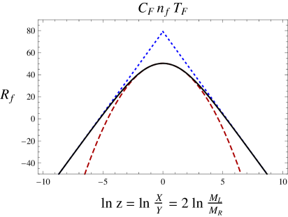
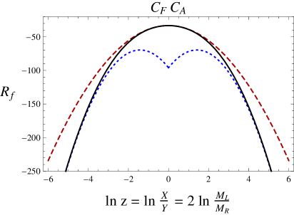
Figure 6: The contribution of the part of the soft function not fixed by renormalization group invariance to the hemisphere mass distribution, ${\mathcal{R}}_{f}(z)$ is shown. On the left is the $C_{F}n_{f}T_{F}$ color factor and on the right is $C_{F}C_{A}$, both as a function of $\ln z\equiv\ln\frac{X}{Y}$. The solid black curve is the exact result of Eq. (6). The dashed red curve is the plot of the small $\ln z$ expression of Eq. (7) and the dotted blue curve give the large $\ln z$ behavior of Eq. (60). The kink is due to a sign flip, since the linear term appears as $|\ln z|$.

Next, let us look at $z\sim 1$. Here we find

$${\mathcal{R}}_{f}^{z\sim 1}(z)=\frac{\pi^{4}}{2}C_{F}^{2}+\left[\left(-\frac{2}{3}-\frac{4\pi^{2}}{3}-4\ln^{2}2+\frac{44\ln 2}{3}\right)\ln^{2}z-32\text{Li}_{4}\left(\frac{1}{2}\right)+\frac{88\zeta_{3}}{9}\right.$$

$$\qquad\left.-28\zeta_{3}\ln(2)-\frac{2032}{81}-\frac{871\pi^{2}}{54}+\frac{16\pi^{4}}{9}-\frac{4\ln^{4}2}{3}+\frac{4}{3}\pi^{2}\ln^{2}2\right]C_{F}C_{A}$$

$$\qquad+\left[\left(\frac{4}{3}-\frac{16\ln 2}{3}\right)\ln^{2}z+\frac{154\pi^{2}}{27}-\frac{136}{81}-\frac{32\zeta_{3}}{9}\right]C_{F}n_{f}T_{F}+\mathcal{O}(\ln^{3}z).$$ (61)

We see there is a double logarithmic term for both the $C_{F}C_{A}$ and $C_{F}n_{f}T_{F}$ color structures. This is consistent with an analysis performed in [15] of an observable $\rho^{\alpha}=\max(\alpha M_{L}^{2},M_{R}^{2})/Q^{2}$. They found that the integrated $\rho^{\alpha}$ distribution looked like $\ln^{2}\alpha$ for $\alpha\sim 1$. This quadratic behavior in $\ln\alpha$ corresponds exactly to the quadratic behavior in the $z\sim 1$ limit in (7).

We show in Figure 6 the exact finite function ${\mathcal{R}}_{f}(z)$ and a comparison to its asymptotic behavior at small $\ln z$ and large $\ln z$ for the $C_{F}C_{A}$ and $C_{F}n_{f}T_{F}$ color structures. For both color structures, the exact curve is well approximated by a parabola for small $\ln z$. At large $\ln z$, for the $C_{F}n_{f}T_{F}$ color factor, the exact result approaches a linear function whereas the $C_{F}C_{A}$ color structure has $\ln^{2}z$ dependence with a different coefficient than for the small $\ln z$ limit. The $C_{F}C_{A}$ term has a linear term as well.

As we have discussed, the integrated hemisphere soft function contributes directly to the doubly differential hemisphere mass distribution. In the limit where both hemisphere masses are small, and well separated, the soft function gives the dominant contribution. In this regime, we can read off that the leading non-global logarithms are given by ${\mathcal{R}}_{f}^{z\gg 1}(M_{L}^{2}/M_{R}^{2})$ in Eq.(60). The $\ln^{2}$ term has an identical coefficient to that found in [26]. The subleading non-global logarithm is a new result.

8 Exponentiation

These non-global logarithms become important when one scale becomes parametrically larger than the other. The separation of scales suggest that at the higher of the two scales, one may be able to match onto a new effective theory and then run the matching coefficient between the two scales. In fact, the $-\frac{4\pi^{2}}{3}\ln^{2}z$ term in this calculation has its origin in $f(0,0)$, where $f(r,\epsilon)$ is the opposite-direction contribution to the hemisphere soft function, as in the Appendix. Indeed, we found that

$$f_{C_{A}}(0,\epsilon)=\frac{8\pi^{2}}{3}+\mathcal{O}(\epsilon),\qquad f_{nf}(0,\epsilon)=\mathcal{O}(\epsilon^{2}),$$ (62)

which is consistent with the leading non-global logarithm only having the $C_{F}C_{A}$ color structure. Since it is the $\epsilon^{0}$ part of this expression which contributes, and there are double soft poles, the full expansion also has terms like $f(0,0)\ln^{2}\mu$. Thus $f(0,0)$ can be thought of as an anomalous dimension, providing hope that these non-global logs might be resummed in an effective theory. A consistent framework may require some kind of refactorization, like the one found for a related event shape, $\tau_{\omega}$, in [25]. Ideas along these lines were suggested in talks by Chris Lee [30, 31]. Lee and collaborators proposed that the leading non-global logs might be resummed with effective field theory, although no details were given.

There is actually good reason to believe the resummation of non-global logs is more challenging than the types of resummation done in SCET. To see this, we first consider the predictions from non-Abelian exponentiation. Non-Abelian exponentiation applies only to the case of pure QCD, without fermion loops. In this case, it says that the full soft function, in Laplace space, can be written as an exponential of 2-particle irreducible diagrams. At order $\alpha_{s}^{n}$, new contributions can appear only to the maximally non-Abelian color structure, $C_{F}C_{A}^{n-1}$. For example, at two-loops, this tells us that the $C_{F}^{2}$ color structure is given entirely by the exponential of the one-loop $C_{F}$ color structure. At 3-loops it predicts the entire $C_{F}^{3}$ and $C_{F}^{2}C_{A}$ color structures.

To be more specific, the soft function in Laplace space factorizes as in Eq. (53), with the $\widetilde{s}_{\mu}$ terms and the $\widetilde{s}_{f}$ terms separately exponentiating, as explained in [15]. So we can write

$$\widetilde{s}_{f}(x_{L},x_{R})=\exp\left[\frac{\alpha_{s}}{4\pi}(-\pi^{2})C_{F}+\left(\frac{\alpha_{s}}{4\pi}\right)^{2}\left(C_{F}n_{f}T_{F}\widetilde{s}_{f}^{(2,n_{f})}(x_{L},x_{R})+C_{F}C_{A}\widetilde{s}_{f}^{(2,C_{A})}(x_{L},x_{R})\right)+\cdots\right]$$ (63)

where $\widetilde{s}_{f}^{(2,n_{f})}$ and $\widetilde{s}_{f}^{(2,C_{A})}$ are the Laplace transforms of the $C_{F}n_{f}T_{F}$ and $C_{F}C_{A}$ color structures in the 2-loop soft function. Such a rewriting has no content unless there is some restriction on the terms appearing in the exponent. Non-Abelian exponentiation tells us that the higher-order terms with $C_{F}$ and $C_{A}$’s only must be maximally non-Abelian, $C_{F}C_{A}^{n-1}$.

This implies, for example, that at 3-loops we know 2 color structures. Explicitly,

$$\widetilde{s}_{f}^{~{}\text{3-loop}}(x_{L},x_{R})=\left(\frac{\alpha_{s}}{4\pi}\right)^{3}\left[C_{F}^{3}\frac{(-\pi^{2})^{3}}{6}+C_{F}^{2}C_{A}(-\pi^{2})\widetilde{s}_{f}^{(2,C_{A})}(x_{L},x_{R})+\cdots\right]$$ (64)

There are 4 remaining color structures, $C_{F}C_{A}^{2}$, $C_{F}n_{f}^{2}T_{F}^{2}$, $C_{F}C_{A}n_{f}T_{F}$ and $C_{F}^{2}n_{f}T_{F}$ which are still unknown. Actually, the $C_{F}n_{f}^{2}T_{F}^{2}$ color structure at 3-loops should not be hard to compute, but there is no known general formula for how the $n_{f}$ color structures exponentiate (see [35] for some discussion).

From the exponentiation formula, one can read off the missing parts of the soft contribution to the 3-loop thrust and heavy-jet mass distributions. Indeed, for $n\geq 2$, we have

$$c^{S}_{n}=C_{F}^{n}\frac{(-\pi^{2})^{n}}{n!}+C_{F}^{n-1}C_{A}\frac{(-\pi^{2})^{n-2}}{(n-2)!}\left[{c^{S}_{2}}\Big{|}_{C_{F}C_{A}}\right]+\cdots\,,$$ (65)

and similarly for $c^{2}_{n\rho}$, with ${c^{S}_{2}}$ and ${c^{S}_{2\rho}}$ given in Eqs. (5) and (5). These constants can be included in future $\alpha_{s}$ fits or, once the finite part of the 3-loop jet function is computed, compared to extractions from the full thrust distrubtion at NNLO [36].

Returning to the exponentiation of non-global logs, recall that the leading non-global log comes from $\widetilde{s}_{f}^{(2,C_{A})}(x_{L},x_{R})=-\frac{4\pi^{2}}{3}L^{2}$, with $L=\ln\frac{x_{L}}{x_{R}}$. Thus non-Abelian exponentiation predicts a series with terms $(C_{F}C_{A}\alpha_{s}^{2}L^{2})^{n-1}$, as well as cross-terms with the $C_{F}$ one-loop color structure which are subleading. The question is whether this is the entire resummation of the leading non-global log. It seems like the answer is no, since there is no apparent reason why 3-loop graphs cannot produce terms which scale like $\alpha_{s}^{3}C_{F}C_{A}^{2}L^{3}$ (or even $\alpha_{s}^{3}L^{4}$) for large $L$. A clue that these terms do exist comes from the numerical resummation of the leading non-global log at large $N_{c}$ in [26]. These authors found that the resummed distribution could be fit by an exponential, but it is numerically different from the pure $(C_{F}C_{A}\alpha_{s}^{2}L^{2})^{n-1}$ terms predicted by Eq. (63). Since $C_{F}$ and $C_{A}$ both scale as $N_{c}$ at large $N_{c}$, this implies that there must be a $\alpha_{s}^{3}C_{F}C_{A}^{2}L^{3}$ term at 3-loops (and no $\alpha_{s}^{3}L^{4}$ term). Thus the resummation of even the leading non-global log may require a way to predict arbitrarily complicated color structures. It would be exciting to see how this can be done in the effective field theory framework.

9 Conclusions

In this paper, we have presented the complete calculation of the hemisphere soft function to order $\alpha_{s}^{2}$. This is the first 2-loop calculation of a soft function which depends on two scales in addition to the renormalization group scale $\mu$. The hemisphere soft function, $S(k_{L},k_{R},\mu)$, depends on the components of the momenta going into the left and right hemispheres. In a one-scale soft function, such as the Drell-Yan soft function, $S_{DY}(k,\mu)$ [22, 23, 32], the thrust soft function $S_{T}(k,\mu)$ [9, 11] or the direct photon soft function $S_{\gamma}(k,\mu)$ [16], all of the $k$ dependence is fixed once the $\mu$-dependence is known. Since the $\mu$-dependence is fixed by RG invariance, these functions are often completely determined. For multi-scale soft functions, like the hemisphere soft function, there can be additional dependence on the ratio $r=k_{L}/k_{R}$. We worked out this dependence explicitly at order $\alpha_{s}^{2}$, and the result is more complicated than previously anticipated.

We performed a number of checks on our calculation. The $\mu$-dependence of the result was entirely known by virtue of the factorization theorem in SCET, and we have confirmed that the $\mu$-dependence of our hemisphere soft function matches the result obtained from factorization analysis. In addition, the result allows us to produce analytic expressions for all of the singular terms in the 2-loop thrust and heavy jet mass distributions. The constant terms in the singular distributions were previously unknown and had to be extracted from numerical fits [11, 15, 12]. We found our analytical results to be in excellent agreement with the very precise recent numerical fit of [12].

The full hemisphere soft function produces the leading and sub-leading non-global logs in the hemisphere mass distribution. Previously, only the leading double-log term was known, from a calculation in the soft limit of full QCD [26]. In this work we reproduced that double logarithm and, furthermore, showed the existence of a sub-leading single logarithm. This single logarithm, of $M_{L}/M_{R}$, is interesting because $\ln M_{L}/M_{R}$ seems like it should be forbidden by the $M_{L}\leftrightarrow M_{R}$ symmetry. Curiously, we find that the complicated behavior of the hemisphere mass distribution when $M_{L}\sim M_{R}$ allows the single log to flip sign and it manifests itself as $\ln[\max(M_{L},M_{R})/\min(M_{L},M_{R})]=|\ln M_{L}/M_{R}|$. Our calculation is the first to exhibit a sub-leading non-global logarithm of this type.

Besides being of formal interest, the hemisphere soft function at $\mathcal{O}(\alpha_{s}^{2})$ is a crucial component of the resummed heavy-jet mass distribution at N³LL order. Previous fits to $\alpha_{s}$ at this order assumed a simple form for the soft function, using the Hoang-Kluth ansatz. We have shown that this ansatz is valid only in the limit that $k_{L}\sim k_{R}$. With the exact $\mathcal{O}(\alpha_{s}^{2})$ soft function in hand, one source of uncertainty in the $\alpha_{s}$ fits to event shapes can be removed.

This work also has implications for calculations of distributions at hadron colliders. At hadron colliders, there are necessarily many more scales in relevant observables than at $e^{+}e^{-}$ machines. For example, jet sizes and veto scales play a critical role in many analysis [33, 19, 25]. For multi-scale observables to be computed in effective field theory, we need a better understanding of multi-scale soft functions, such as this exact result on the 2-loop hemisphere soft function provides.

10 Acknowledgements

The authors would like to thank Y.-T. Chien, M. Dasgupta, C. Lee, K. Melnikov, G. Salam and I. Stewart for useful discussions and F. Petriello and I. Scimemi for collaboration on intermediate stages of this project. RK and MDS were supported in part by the Department of Energy, under grant DE-SC003916. HXZ was supported by the National Natural Science Foundation of China under grants No. 11021092 and No. 10975004 and the Graduate Student academic exchange program of Peking University.

Appendix A Opposite direction contributions

The following are the first 3 terms in the $\epsilon$ expansion of $f_{C_{A}}$ from Eq. (22).

$$f_{C_{A}}^{(0)}(r) =8\left(\frac{r\left(11r^{2}+21r+12\right)\ln(r)}{3(r+1)^{3}}+\frac{\pi^{2}(r+1)^{2}+2r}{3(r+1)^{2}}+\ln^{2}(r+1)\right.$$

$$\qquad\left.-\ln(r)\ln(r+1)-\frac{11}{3}\ln(r+1)\right),$$ (66)

$$f_{C_{A}}^{(1)}(r) =\frac{8\left(-11r^{3}-9r^{2}+9r+11\right)\text{Li}_{2}(-r)}{3(r+1)^{3}}+24\text{Li}_{3}(-r)-16\text{Li}_{2}(-r)\log(r)$$

$$+\frac{4r\left(11r^{2}+21r+12\right)\log^{2}(r)}{3(r+1)^{3}}-\frac{8r\left(67r^{2}+141r+60\right)\log(r)}{9(r+1)^{3}}$$

$$-\frac{4\left(r^{3}\left(11\pi^{2}-36\zeta(3)\right)+r^{2}\left(-108\zeta(3)+32+21\pi^{2}\right)+4r\left(-27\zeta(3)+8+3\pi^{2}\right)-36\zeta(3)\right)}{9(r+1)^{3}}$$

$$+\frac{8\left(-11r^{3}-9r^{2}+9r+11\right)\ln(r+1)\ln(r)}{3(r+1)^{3}}-4\ln(r+1)\ln^{2}(r)+\frac{4}{9}\left(134+3\pi^{2}\right)\ln(r+1),$$ (67)

$$f_{C_{A}}^{(2)}(r) =\frac{8\left(67r^{3}+81r^{2}-81r-67\right)\text{Li}_{2}(-r)}{9(r+1)^{3}}-\frac{8\left(55r^{3}+117r^{2}+81r+11\right)\text{Li}_{3}(-r)}{3(r+1)^{3}}$$

$$-\frac{32\left(11r^{3}+9r^{2}-9r-11\right)\text{Li}_{3}\left(\frac{1}{r+1}\right)}{3(r+1)^{3}}-\frac{16\left(11r^{3}+9r^{2}-9r-11\right)\text{Li}_{2}(-r)\ln(r+1)}{3(r+1)^{3}}$$

$$+\frac{8\left(33r^{3}+75r^{2}+57r+11\right)\text{Li}_{2}(-r)\ln(r)}{3(r+1)^{3}}-16\text{Li}_{4}\left(\frac{1}{r+1}\right)-16\text{Li}_{4}\left(\frac{r}{r+1}\right)$$

$$-8\text{Li}_{2}(-r)\ln^{2}(r)+16\text{Li}_{2}(-r)\ln(r)\ln(r+1)+8\text{Li}_{3}(-r)\ln(r)+16\text{Li}_{3}\left(\frac{1}{r+1}\right)\ln(r)$$

$$+\frac{4\left(-40\left(4r^{2}(27\zeta(3)-2)+r(189\zeta(3)-8)+99\zeta(3)\right)+5\pi^{2}r\left(67r^{2}+147r+66\right)+33\pi^{4}(r+1)^{3}\right)}{135(r+1)^{3}}$$

$$-\frac{32\left(12r^{2}+21r+11\right)\ln^{3}(r+1)}{9(r+1)^{3}}+\frac{4r\left(11r^{2}+21r+12\right)\ln^{3}(r)}{9(r+1)^{3}}-\frac{4}{3}\ln^{3}(r)\ln(r+1)$$

$$+\frac{16\left(12r^{2}+21r+11\right)\ln(r)\ln^{2}(r+1)}{3(r+1)^{3}}-\frac{4r\left(67r^{2}+141r+60\right)\ln^{2}(r)}{9(r+1)^{3}}$$

$$+\frac{16r\left(193r^{2}+384r+177\right)\ln(r)}{27(r+1)^{3}}+\frac{4\left(-11r^{3}-9r^{2}+9r+11\right)\ln^{2}(r)\ln(r+1)}{3(r+1)^{3}}$$

$$-\frac{8\left(\pi^{2}\left(66r^{3}+90r^{2}+9r-33\right)+2\left(193r^{3}+561r^{2}+561r+193\right)\right)\ln(r+1)}{27(r+1)^{3}}$$

$$+\frac{8\left(67r^{3}+69r^{2}-93r+3\pi^{2}(r+1)^{3}-67\right)\ln(r)\ln(r+1)}{9(r+1)^{3}}-\frac{4}{3}\ln^{4}(r+1)$$

$$+8\ln^{2}(r)\ln^{2}(r+1)+16\zeta(3)\ln(r+1)-16\zeta(3)\log(r)+\frac{32r\ln^{2}(r+1)}{3(r+1)^{2}}.$$ (68)

The following are the first 2 terms in the $\epsilon$ expansion of $f_{n_{f}}$ from Eq. (34).

$$f_{n_{f}}^{(0)}(r) =-\frac{16\left(2r(r+1)-2(r+1)^{3}\ln(r+1)+r(r(2r+3)+3)\ln(r)\right)}{3(r+1)^{3}},$$ (69)

$$f_{n_{f}}^{(1)}(r) =\frac{8}{9(r+1)^{3}}\left(-12\left(r^{3}-1\right)\text{Li}_{2}\left(-\frac{1}{r}\right)-32r^{3}\ln(r+1)+3\pi^{2}r^{2}+20r^{2}\right.$$

$$\quad\left.-96r^{2}\ln(r+1)-3\left(4r^{3}+3r^{2}+3r-2\right)\ln^{2}(r)+4\ln(r)\left(3\left(r^{3}-1\right)\ln(r+1)\right.\right.$$

$$\quad\left.\left.+r\left(8r^{2}+21r+3\right)\right)+3\pi^{2}r+20r-96r\ln(r+1)-32\ln(r+1)+2\pi^{2}\right).$$ (70)

References

- [1] A. Gehrmann-De Ridder, T. Gehrmann and E. W. N. Glover, JHEP 0509, 056 (2005) [arXiv:hep-ph/0505111].
- [2] A. Gehrmann-De Ridder, T. Gehrmann, E. W. N. Glover and G. Heinrich, Phys. Rev. Lett. 99, 132002 (2007) [arXiv:0707.1285 [hep-ph]].
- [3] A. Gehrmann-De Ridder, T. Gehrmann, E. W. N. Glover and G. Heinrich, JHEP 0712, 094 (2007) [arXiv:0711.4711 [hep-ph]].
- [4] S. Weinzierl, Phys. Rev. Lett. 101, 162001 (2008) [arXiv:0807.3241 [hep-ph]].
- [5] C. W. Bauer, S. Fleming, D. Pirjol and I. W. Stewart, Phys. Rev. D 63, 114020 (2001) [arXiv:hep-ph/0011336].
- [6] C. W. Bauer, D. Pirjol and I. W. Stewart, Phys. Rev. D 65, 054022 (2002) [arXiv:hep-ph/0109045].
- [7] M. Beneke, A. P. Chapovsky, M. Diehl and T. Feldmann, Nucl. Phys. B 643, 431 (2002) [arXiv:hep-ph/0206152].
- [8] S. Fleming, A. H. Hoang, S. Mantry and I. W. Stewart, Phys. Rev. D 77, 074010 (2008) [arXiv:hep-ph/0703207].
- [9] M. D. Schwartz, Phys. Rev. D 77, 014026 (2008) [arXiv:0709.2709 [hep-ph]].
- [10] T. Becher and M. Neubert, Phys. Lett. B 637, 251 (2006) [arXiv:hep-ph/0603140].
- [11] T. Becher and M. D. Schwartz, JHEP 0807, 034 (2008) [arXiv:0803.0342 [hep-ph]].
- [12] Y. T. Chien and M. D. Schwartz, JHEP 1008, 058 (2010) [arXiv:1005.1644 [hep-ph]].
- [13] R. Abbate, M. Fickinger, A. H. Hoang, V. Mateu, I. W. Stewart, Phys. Rev. D83, 074021 (2011). [arXiv:1006.3080 [hep-ph]].
- [14] W. M. Yao et al. [Particle Data Group], J. Phys. G 33, 1 (2006).
- [15] A. H. Hoang and S. Kluth, arXiv:0806.3852 [hep-ph].
- [16] T. Becher and M. D. Schwartz, JHEP 1002, 040 (2010) [arXiv:0911.0681 [hep-ph]].
- [17] N. Kidonakis, G. F. Sterman, Nucl. Phys. B505, 321-348 (1997). [hep-ph/9705234].
- [18] S. M. Aybat, L. J. Dixon, G. F. Sterman, Phys. Rev. D74, 074004 (2006). [hep-ph/0607309].
- [19] S. D. Ellis, C. K. Vermilion, J. R. Walsh, A. Hornig and C. Lee, arXiv:1001.0014 [hep-ph].
- [20] R. Kelley, M. D. Schwartz, Phys. Rev. D83, 033001 (2011). [arXiv:1008.4355 [hep-ph]].
- [21] R. Kelley, M. D. Schwartz, Phys. Rev. D83, 045022 (2011). [arXiv:1008.2759 [hep-ph]]. ,1002,040;
- [22] G. P. Korchemsky and G. Marchesini, Phys. Lett. B 313, 433 (1993).
- [23] A. V. Belitsky, Phys. Lett. B 442, 307 (1998) [arXiv:hep-ph/9808389].
- [24] T. Becher and M. Neubert, Phys. Lett. B 633, 739 (2006) [arXiv:hep-ph/0512208].
- [25] R. Kelley, M. D. Schwartz and H. X. Zhu, arXiv:1102.0561 [hep-ph].
- [26] M. Dasgupta and G. P. Salam, Phys. Lett. B 512, 323 (2001) [arXiv:hep-ph/0104277].
- [27] S. Fleming, A. H. Hoang, S. Mantry and I. W. Stewart, Phys. Rev. D 77, 114003 (2008) [arXiv:0711.2079 [hep-ph]].
- [28] T. Huber and D. Maitre, Comput. Phys. Commun. 175, 122 (2006) [arXiv:hep-ph/0507094].
- [29] G. Heinrich, Int. J. Mod. Phys. A 23, 1457 (2008) [arXiv:0803.4177 [hep-ph]].
- [30] C. Lee, A. Hornig, I. W. Stewart, J. R. Walsh, and S. Zuberi, “Non-Global Logs in SCET.” Talk presented at SCET 2011 Workshop, March 6–8, 2011, Carnegie Mellon University.
- [31] C. Lee, A. Hornig, I. W. Stewart, J. R. Walsh, and S. Zuberi, “Non-Global Logs in SCET.” Talk presented at BOOST 2011 Workshop, May 22-26, 2011, Princeton NJ.
- [32] T. Becher, M. Neubert and G. Xu, JHEP 0807, 030 (2008) [arXiv:0710.0680 [hep-ph]].
- [33] S. D. Ellis, A. Hornig, C. Lee, C. K. Vermilion, J. R. Walsh, Phys. Lett. B689, 82-89 (2010). [arXiv:0912.0262 [hep-ph]].
- [34] A. Hornig, C. Lee, I. W. Stewart, J. R. Walsh, S. Zuberi, [arXiv:1105.4628 [hep-ph]].
- [35] C. F. Berger, Phys. Rev. D 66, 116002 (2002) [arXiv:hep-ph/0209107].
- [36] P. F. Monni, T. Gehrmann, G. Luisoni, [arXiv:1105.4560 [hep-ph]].