Perturbation analysis of Mode III interfacial cracks advancing in a dilute heterogeneous material

Abstract

The paper addresses the problem of a Mode III interfacial crack advancing quasi-statically in a heterogeneous composite material, that is a two-phase material containing elastic inclusions, both soft and stiff, and defects, such as microcracks, rigid line inclusions and voids. It is assumed that the bonding between dissimilar elastic materials is weak so that the interface is a preferential path for the crack. The perturbation analysis is made possible by means of the fundamental solutions (symmetric and skew-symmetric weight functions) derived in Piccolroaz et al. (2009). We derive the dipole matrices of the defects in question and use the corresponding dipole fields to evaluate effective tractions along the crack faces and interface to describe the interaction between the main interfacial crack and the defects. For a stable propagation of the crack, the perturbation of the stress intensity factor induced by the defects is then balanced by the elongation of the crack along the interface, thus giving an explicit asymptotic formula for the calculation of the crack advance. The method is general and applicable to interfacial cracks with general distributed loading on the crack faces, taking into account possible asymmetry in the boundary conditions.

The analytical results are used to analyse the shielding and amplification effects of various types of defects in different configurations. Numerical computations based on the explicit analytical formulae allows for the analysis of crack propagation and arrest.

1 Introduction

Analytic solutions for a crack propagating in a homogeneous elastic solid containing a finite number of small defects (elastic and rigid inclusions, microcracks, voids) have been derived in Bigoni et al. (1998), Valentini et al. (1999), Movchan et al. (2002) on the basis of the dipole matrix and weight function approach. The dipole field describes the leading-order perturbation produced by a small defect placed in a smooth stress field and gives rise to “effective” tractions applied along the crack faces. Furthermore, the weight functions allow for the derivation of the corresponding perturbation of the stress intensity factor as weighted integral of the “effective” loading. The method is general and applicable to both 2D and 3D cases and to defects of different type and shape, provided that the corresponding dipole matrix is appropriately constructed and the weight functions for the corresponding unperturbed cracked body are available.

Problems of a macrocrack interacting with microcracks have been analysed by Romalis and Tamuzh (1984) under the influence of mechanical loading and by Tamusz et al. (1993) under the influence of heat flux, using the analytic functions and singular integrals approach (Muskhelishvili, 2008). The possible closure of crack surfaces and the consequent appearance of a contact zone have been considered in Tamuzs et al. (1994) and Tamuzs et al. (1996). Asymptotic models of a semi-infinite crack interacting with microcracks have been developed by Gong and Horii (1989) and Meguid et al. (1991) using complex potentials and the superposition principle. A review of publications on macro–microcrack interaction problem is given in Tamuzs and Petrova (2002).

Recently, Piccolroaz et al. (2009) derived the symmetric and skew-symmetric weight functions for a semi-infinite two-dimensional interfacial crack, thus disclosing the possibility of applying the dipole matrix approach to the propagation of cracks along the interface in heterogeneous materials with small defects. The weight functions constructed in Piccolroaz et al. (2009) are of the generalised type and thus applicable to any type of boundary conditions along the crack faces. The singular perturbation associated with a small crack advance was also obtained there. It is worth noting that the availability of the skew-symmetric function for the problem under consideration is essential since the “effective” loading produced by the defects on the crack faces is not symmetrical, in general. In the present paper, we analyse the scalar case of antiplane shear loading. The full vector problem will be addressed elsewhere.

The paper is organised as follows. The formulation of the problem is outlined in Section 2, which includes also preliminary results on the unperturbed problem. Section 3 is devoted to the perturbation analysis, in particular the derivation of the dipole fields for several types of defects and the analysis of singular perturbation associated with the crack advance. Section 4 provides a number of numerical results based on the explicit analytical formulae. In particular, shielding and amplification effects of different defect configurations on the crack-tip field are presented. The possibility to design a neutral configuration for any given force system distributed along the crack faces is discussed. Finally, the crack propagation and arrest produced by the defects under consideration is analysed. In the appendix, we derive the dipole matrix for an elliptic elastic inclusion placed in a homogeneous antiplane field.

2 Problem formulation and preliminary results

We consider a two-dimensional composite structure consisting of a bimaterial matrix (two dissimilar elastic half-planes $\Omega_{\pm}$) containing a dilute distribution of inclusions, microcracks and rigid line inclusions, see Fig. 1. The two materials constituting the matrix are assumed to be linear elastic and isotropic, with shear moduli denoted by $\mu_{+}$ and $\mu_{-}$, respectively. All interfaces between different phases are assumed to be perfect, that is, the displacements and tractions remain continuous across the interface.

We introduce the following notations. Let $g_{\varepsilon}\subset\Omega_{+}$ be a small elastic inclusion of diameter $2\varepsilon l_{1}$ centred at the point $\mbox{\boldmath$Y$}_{1}=(a_{1},h_{1})$. The shear modulus of the inclusion is denoted by $\mu_{i}$, and it can be greater or smaller than the shear modulus $\mu_{+}$ of the surrounding material, so that both stiff and soft inclusions are considered. The notation $\gamma_{2}^{\varepsilon}\subset\Omega_{-}$ is used for a microcrack of the length $2\varepsilon l_{2}$, centred at the point $Y_{2}=(a_{2},h_{2})$ and making an angle $\alpha_{2}>0$ with the positive direction of the $x_{1}$-axis. By $\gamma_{3}^{\varepsilon}\subset\Omega_{+}$ we denote a movable rigid line inclusion of the length $2\varepsilon l_{3}$, centred at the point $Y_{3}=(a_{3},h_{3})$ and making an angle $\alpha_{3}>0$ with the positive direction of the $x_{1}$-axis. Although these notations refer specifically to Fig. 1, the formulation can be easily extended to problems with different number and type of defects, as those considered in Sec. 4.

We assume that a semi-infinite interface crack $M_{\varepsilon}$ advances quasi-statically along the interface $\Gamma_{\varepsilon}$ connecting the half-planes, and we denote the uniform advance of the crack by $\varepsilon^{2}\phi$. Here and in the sequel, $\varepsilon>0$ is a small dimensionless parameter. The reason for the order $\varepsilon^{2}$ in the crack advance will be clear in Sec. 3, where we perform the asymptotic analysis.

Figure 1: Geometry of the problem: interface crack in a bimaterial plane with defects: $g_{\varepsilon}$ denotes a small elastic inclusion, $\gamma_{2}^{\varepsilon}$ a microcrack, and $\gamma_{3}^{\varepsilon}$ a rigid line inclusion; $\mbox{\boldmath$Y$}_{1},\mbox{\boldmath$Y$}_{2},\mbox{\boldmath$Y$}_{3}$ are the “centres” of the defects.

We assume that the composite is dilute, that is, the small defects are distant from each other so that the interaction between them can be neglected. Consequently, we can model the three cases of an elastic inclusion, of a microcrack and of a rigid line inclusion separately. It is possible then to extend the results to a finite number of defects by superposition using the linearity of the problem, provided that the distance between defects remains finite.

An external loading $p_{\pm}$ is applied to the crack faces $\Gamma_{\pm}^{\varepsilon}$ and it is assumed to be self-balanced such that the principal force vector is zero, that is,

$$\int_{\Gamma_{+}^{\varepsilon}}p_{+}d\mbox{\boldmath$x$}-\int_{\Gamma_{-}^{\varepsilon}}p_{-}d\mbox{\boldmath$x$}=0.$$ (1)

We assume that the loading $p_{\pm}$ on the crack faces vanishes in a neighbourhood of the crack tip.

The problem is then formulated in terms of the Laplace equation

$$\Delta u_{\pm}(x_{1},x_{2})=0,\quad\Delta u_{i}(x_{1},x_{2})=0,$$ (2)

where $u=\{u_{+},u_{-},u_{i}\}$ denotes the displacement component along $x_{3}$-axis in the respective domain $\Omega_{+}\setminus\{g_{\varepsilon}\cup\gamma_{3}^{\varepsilon}\}$, $\Omega_{-}\setminus\gamma_{2}^{\varepsilon}$ and $g_{\varepsilon}$.

We prescribe the following boundary conditions on the crack faces

$$\mu_{\pm}\frac{\partial u_{\pm}}{\partial x_{2}}=p_{\pm}\quad\text{on $\Gamma_{\pm}^{\varepsilon}$},$$ (3)

and the interface conditions

$$u_{+}=u_{-},\quad\mu_{+}\frac{\partial u_{+}}{\partial x_{2}}=\mu_{-}\frac{\partial u_{-}}{\partial x_{2}}\quad\text{on $\Gamma^{\varepsilon}$}.$$ (4)

The transmission conditions for the elastic inclusion $g_{\varepsilon}$ are formulated similarly to (4), that is,

$$u_{+}=u_{i},\quad\mu_{+}\frac{\partial u_{+}}{\partial n}=\mu_{i}\frac{\partial u_{i}}{\partial n}\quad\text{on $\partial g_{\varepsilon}$}.$$ (5)

We assume that the microcrack faces $\gamma_{2}^{\pm}$ are traction free, so that

$$\frac{\partial u_{-}}{\partial n}=0\quad\text{on}\quad\gamma_{2}^{\pm}.$$ (6)

Finally, on the boundary of the movable rigid line inclusion $\gamma_{3}^{\varepsilon}$ the Dirichlet boundary condition is prescribed, that is,

$$u_{+}=u_{*}\quad\text{on}\quad\gamma_{3}^{\varepsilon},$$ (7)

where $u_{*}$ is an unknown constant which will be defined later from the balance condition

$$\int_{\gamma_{3}^{\varepsilon}}\frac{\partial u_{+}}{\partial n}ds=0.$$ (8)

The unperturbed problem ($\varepsilon=0$) corresponds to a semi-infinite interfacial crack in a bimaterial plane. The solution to this problem (see, for example, Piccolroaz et al. 2010) can be expressed in the form

$$u_{\pm}^{(0)}(r,\theta)=\frac{1}{2\pi i}\int_{\omega-i\infty}^{\omega+i\infty}\tilde{u}_{\pm}^{(0)}(s,\theta)r^{-s}ds,\quad\pm\theta\in(0,\pi),$$ (9)

where

$$\tilde{u}^{(0)}_{\pm}(s,\theta)=-\frac{\sin(s\theta)}{\mu_{\pm}s\cos(\pi s)}\langle\tilde{p}\rangle(s)+\left[\frac{\cos(s\theta)}{(\mu_{+}+\mu_{-})s\sin(\pi s)}+\frac{(\mu_{+}-\mu_{-})\sin(s\theta)}{2\mu_{\pm}(\mu_{+}+\mu_{-})s\cos(\pi s)}\right][\mbox{}[\tilde{p}]\mbox{}](s),$$ (10)

and $0<\omega<0.5$, with the symmetric and skew-symmetric components of the loading denoted by $[\mbox{}[p]\mbox{}]=p_{+}-p_{-}$ and $\langle p\rangle=(p_{+}+p_{-})/2$, respectively.

The two-terms asymptotic expansions for the traction $\sigma^{(0)}$ ahead of the crack tip and for the crack opening $[\mbox{}[u^{(0)}]\mbox{}]$ read as follows

$$\sigma^{(0)}(r,0)=\frac{K^{(0)}_{\text{III}}}{\sqrt{2\pi}}r^{-1/2}+\frac{A^{(0)}_{\text{III}}}{\sqrt{2\pi}}r^{1/2}+O(r^{3/2}),$$ (11)

$$[\mbox{}[u^{(0)}]\mbox{}](r)=\frac{\mu_{+}+\mu_{-}}{\mu_{+}\mu_{-}}\left(\frac{2K^{(0)}_{\text{III}}}{\sqrt{2\pi}}r^{1/2}-\frac{2A^{(0)}_{\text{III}}}{3\sqrt{2\pi}}r^{3/2}\right)+O(r^{5/2}),$$ (12)

where

$$K^{(0)}_{\text{III}}=-\sqrt{\frac{2}{\pi}}\int_{0}^{\infty}\left\{\langle p\rangle(-r)+\frac{\eta}{2}[\mbox{}[p]\mbox{}](-r)\right\}r^{-1/2}dr,$$ (13)

$$A^{(0)}_{\text{III}}=\sqrt{\frac{2}{\pi}}\int_{0}^{\infty}\left\{\langle p\rangle(-r)+\frac{\eta}{2}[\mbox{}[p]\mbox{}](-r)\right\}r^{-3/2}dr,$$ (14)

with $\eta=(\mu_{-}-\mu_{+})/(\mu_{+}+\mu_{-})$ being the contrast parameter.

For the perturbation analysis we will also need the so-called symmetric and skew-symmetric weight functions, $[\mbox{}[U]\mbox{}]$ and $\langle U\rangle$, respectively, and the corresponding traction $\langle\Sigma\rangle$ in a bimaterial plane with a semi-infinite crack (see Piccolroaz et al., 2009),

$$[\mbox{}[U]\mbox{}](x_{1})=\left\{\begin{array}[]{ll}\displaystyle\frac{1-i}{\sqrt{2\pi}}x_{1}^{-1/2},&\displaystyle x_{1}>0,\\[8.53581pt] 0,&x_{1}<0,\end{array}\right.\quad\langle U\rangle(x_{1})=\eta/2[\mbox{}[U]\mbox{}](x_{1}),$$ (15)

$$\langle\Sigma\rangle(x_{1})=\left\{\begin{array}[]{ll}0,&\displaystyle x_{1}>0,\\[8.53581pt] \displaystyle\frac{(1-i)\mu_{+}\mu_{-}}{2\sqrt{2\pi}(\mu_{+}+\mu_{-})}(-x_{1})^{-3/2},&x_{1}<0.\end{array}\right.$$ (16)

For an arbitrary solution $u$ of the governing equation (2) and the corresponding traction $\sigma$ along the $x_{1}$-axis, the reciprocity identity has the form (Piccolroaz et al., 2009)

$$\int_{-\infty}^{\infty}\Big{\{}[\mbox{}[U]\mbox{}](x_{1}^{\prime}-x_{1})\langle\sigma\rangle(x_{1})+\langle U\rangle(x_{1}^{\prime}-x_{1})[\mbox{}[\sigma]\mbox{}](x_{1})-\langle\Sigma\rangle(x_{1}^{\prime}-x_{1})[\mbox{}[u]\mbox{}](x_{1})\Big{\}}dx_{1}=0,$$ (17)

where the following notations have been used:

$$[\mbox{}[f]\mbox{}]=f_{+}-f_{-},\quad\langle f\rangle=\frac{1}{2}(f_{+}+f_{-}).$$

Let us introduce the notations

$$f^{(+)}(x_{1})=f(x_{1})H(x_{1}),\quad f^{(-)}(x_{1})=f(x_{1})H(-x_{1}),$$

where $H$ denotes the Heaviside function, so that

$$f(x_{1})=f^{(+)}(x_{1})+f^{(-)}(x_{1}).$$ (18)

The reciprocity identity (17) can be written as

$$\begin{array}[]{l}\displaystyle\int_{-\infty}^{\infty}\left\{[\mbox{}[U]\mbox{}](x_{1}^{\prime}-x_{1})\langle\sigma\rangle^{(+)}(x_{1})-\langle\Sigma\rangle(x_{1}^{\prime}-x_{1})[\mbox{}[u]\mbox{}]^{(-)}(x_{1})\right\}dx_{1}=\\[8.53581pt] \displaystyle-\int_{-\infty}^{\infty}\left\{[\mbox{}[U]\mbox{}](x_{1}^{\prime}-x_{1})\langle\sigma\rangle^{(-)}(x_{1})+\langle U\rangle(x_{1}^{\prime}-x_{1})[\mbox{}[\sigma]\mbox{}]^{(-)}(x_{1})\right\}dx_{1}\\[8.53581pt] \displaystyle-\int_{-\infty}^{\infty}\langle U\rangle(x_{1}^{\prime}-x_{1})[\mbox{}[\sigma]\mbox{}]^{(+)}(x_{1})dx_{1}+\int_{-\infty}^{\infty}\langle\Sigma\rangle(x_{1}^{\prime}-x_{1})[\mbox{}[u]\mbox{}]^{(+)}(x_{1})dx_{1}.\end{array}$$ (19)

Note that $\langle\sigma\rangle^{(-)}$, $[\mbox{}[\sigma]\mbox{}]^{(-)}$ are the average and the jump of the prescribed loading on the crack faces, whereas $[\mbox{}[\sigma]\mbox{}]^{(+)}$, $[\mbox{}[u]\mbox{}]^{(+)}$ are the prescribed discontinuities of traction and displacement across the interface. The identity (19) will be used extensively later in the perturbation analysis.

Additionally, we shall need the components of the displacement gradient $\nabla_{\mbox{\boldmath$x$}}u_{\pm}^{(0)}$ computed at an arbitrary point $\mbox{\boldmath$Y$}=(d\cos\varphi,d\sin\varphi)$. These are obtained from (9) and given by

$$\begin{array}[]{r}\displaystyle\left.\frac{\partial u_{\pm}^{(0)}}{\partial x_{1}}\right|_{\mbox{\boldmath$Y$}}=\frac{1}{\pi d}\int_{-\infty}^{0}\frac{dx_{1}}{2\cos\varphi-x_{1}/d-d/x_{1}}\left\{\frac{[\mbox{}[p]\mbox{}](x_{1})}{\mu_{+}+\mu_{-}}\left[\vphantom{\sqrt{\frac{-x_{1}}{d}}}\sin^{2}\varphi-\frac{1}{2}\cos\varphi\left(\frac{d}{x_{1}}-\frac{x_{1}}{d}\right)\right]+\right.\\[14.22636pt] \displaystyle\left.+\frac{2\langle p\rangle(x_{1})+\eta[\mbox{}[p]\mbox{}](x_{1})}{2\mu_{\pm}}\left(\sqrt{\frac{-x_{1}}{d}}\sin\frac{\varphi}{2}+\sqrt{\frac{d}{-x_{1}}}\sin\frac{3\varphi}{2}\right)\right\},\end{array}$$ (20)

$$\begin{array}[]{r}\displaystyle\left.\frac{\partial u_{\pm}^{(0)}}{\partial x_{2}}\right|_{\mbox{\boldmath$Y$}}=-\frac{1}{\pi d}\int_{-\infty}^{0}\frac{dx_{1}}{2\cos\varphi-x_{1}/d-d/x_{1}}\left\{\frac{[\mbox{}[p]\mbox{}](x_{1})\sin\varphi}{\mu_{+}+\mu_{-}}\left[\vphantom{\sqrt{\frac{-x_{1}}{d}}}\cos\varphi+\frac{1}{2}\left(\frac{d}{x_{1}}-\frac{x_{1}}{d}\right)\right]+\right.\\[14.22636pt] \displaystyle\left.+\frac{2\langle p\rangle(x_{1})+\eta[\mbox{}[p]\mbox{}](x_{1})}{2\mu_{\pm}}\left(\sqrt{\frac{-x_{1}}{d}}\cos\frac{\varphi}{2}+\sqrt{\frac{d}{-x_{1}}}\cos\frac{3\varphi}{2}\right)\right\}.\end{array}$$ (21)

3 Perturbation analysis

We shall construct an asymptotic solution of the problem using the method of Movchan and Movchan (1995), that is the asymptotics of the solution will be taken in the form

$$u_{\pm}(\mbox{\boldmath$x$},\varepsilon)=u_{\pm}^{(0)}(\mbox{\boldmath$x$})+\varepsilon\sum_{j=1}^{3}W_{j}(\mbox{\boldmath$\xi$}_{j})+\varepsilon^{2}\sum_{j=1}^{3}u_{\pm}^{(j)}(\mbox{\boldmath$x$})+\varepsilon^{2}v(\mbox{\boldmath$x$},\phi)+o(\varepsilon^{2}),\quad\varepsilon\to 0.$$ (22)

In (22), the leading term $u_{\pm}^{(0)}(\mbox{\boldmath$x$})$ corresponds to the unperturbed solution, and it is described in the previous section. The term $\varepsilon\sum_{j=1}^{3}W_{j}(\mbox{\boldmath$\xi$}_{j})$ corresponds to the boundary layers concentrated near the defects and needed to satisfy the respective conditions (5), (6) and (7); the variables $\mbox{\boldmath$\xi$}_{j}$ will be defined in the next section. The term $\varepsilon^{2}\sum_{j=1}^{3}u_{\pm}^{(j)}(\mbox{\boldmath$x$})$ is introduced to fulfil the original boundary conditions (3) on the crack faces and the interface conditions (4) disturbed by the boundary layers; this term, in turn, will produce perturbations of the crack tip fields and correspondingly of the stress intensity factor. In Sec. 3.1 we will analyse the effect of each defect separately. Finally, the term $\varepsilon^{2}v(\mbox{\boldmath$x$},\phi)$ corresponds to a singular perturbation associated with a possible crack advance, $\varepsilon^{2}\phi$, and will be addressed in Sec. 3.2.

3.1 Singular perturbation and dipole fields generated by small defects

3.1.1 Small elastic inclusion

We shall start with the elastic inclusion, situated in the upper half-plane. The leading term $u^{(0)}=u^{(0)}_{+}$ clearly does not satisfy the transmission conditions (5) on the boundary $\partial g_{\varepsilon}$. Thus, we shall correct the solution by constructing the boundary layer $W_{1}(\mbox{\boldmath$\xi$}_{1})$, where the new scaled variable $\mbox{\boldmath$\xi$}_{1}$ is defined by

$$\mbox{\boldmath$\xi$}_{1}=\frac{\mbox{\boldmath$x$}-\mbox{\boldmath$Y$}_{1}}{\varepsilon},$$ (23)

with $\mbox{\boldmath$Y$}_{1}$ being the “centre” of the inclusion $g_{\varepsilon}$ (see Fig. 1).

For $W_{1}(\mbox{\boldmath$\xi$}_{1})=\{W_{1}^{in},\ \mbox{\boldmath$\xi$}_{1}\in g;\ W_{1}^{out},\ \mbox{\boldmath$\xi$}_{1}\in\mathbb{R}^{2}\setminus\overline{g}\}$ we consider the following problem

$$\Delta W_{1}^{in}(\mbox{\boldmath$\xi$}_{1})=0,\quad\mbox{\boldmath$\xi$}_{1}\in g,\quad\Delta W_{1}^{out}=0,\quad\mbox{\boldmath$\xi$}_{1}\in\mathbb{R}^{2}\setminus\overline{g},$$ (24)

where

$$g=\varepsilon^{-1}g_{\varepsilon}\equiv\{\mbox{\boldmath$\xi$}_{1}\in\mathbb{R}^{2}:\varepsilon\mbox{\boldmath$\xi$}_{1}+\mbox{\boldmath$Y$}_{1}\in g_{\varepsilon}\}.$$

The function $W_{1}$ remains continuous across the interface $\partial g$, that is,

$$W_{1}^{in}=W_{1}^{out}\quad\text{on}\quad\partial g,$$

and satisfies on $\partial g$ the following transmission condition

$$\mu_{i}\frac{\partial}{\partial\mbox{\boldmath$n$}}W_{1}^{in}(\mbox{\boldmath$\xi$}_{1})-\mu_{+}\frac{\partial}{\partial\mbox{\boldmath$n$}}W_{1}^{out}(\mbox{\boldmath$\xi$}_{1})=(\mu_{+}-\mu_{i})\mbox{\boldmath$n$}\cdot\nabla u^{(0)}(\mbox{\boldmath$Y$}_{1})+O(\varepsilon),\quad\varepsilon\to 0,$$ (25)

where $\mbox{\boldmath$n$}=\mbox{\boldmath$n$}_{\mbox{\boldmath$\xi$}_{1}}$ is an outward unit normal on $\partial g$. The formulation is completed by setting the following condition at infinity

$$W_{1}^{out}\to 0\quad\text{as}\quad|\mbox{\boldmath$\xi$}_{1}|\to\infty.$$ (26)

The problem above has been solved by various techniques and the solution can be found, for example, in Movchan and Movchan (1995).

Since we assume that the inclusion is at a finite distance from the interface between the half-planes, we shall only need the leading term of the asymptotics of the solution at infinity. This term reads as follows

$$W_{1}^{out}(\mbox{\boldmath$\xi$}_{1})=-\frac{1}{2\pi}\left[\left.\nabla_{\mbox{\boldmath$x$}}\,u^{(0)}\right|_{\mbox{\boldmath$Y$}_{1}}\right]\cdot\left[\mbox{\boldmath$\mathcal{M}$}_{1}\frac{\mbox{\boldmath$\xi$}_{1}}{|\mbox{\boldmath$\xi$}_{1}|^{2}}\right]+O(|\mbox{\boldmath$\xi$}_{1}|^{-2})\quad\text{as}\quad\mbox{\boldmath$\xi$}_{1}\to\infty,$$ (27)

where $\mbox{\boldmath$\mathcal{M}$}_{1}$ is a 2 $\times$ 2 matrix which depends on the characteristic size $l_{1}$ of the domain $g$ and the ratio $\mu_{+}/\mu_{i}$; it is called the dipole matrix. For example, in the case of an elliptic inclusion with the semi-axes $l_{a}$ and $l_{b}$ making an angle $\alpha_{1}$ with the positive direction of the $x_{1}$-axis and $x_{2}$-axis, respectively, the matrix $\mbox{\boldmath$\mathcal{M}$}_{1}$ takes the form

$$\mbox{\boldmath$\mathcal{M}$}_{1}=-\frac{\pi}{2}l_{a}l_{b}(1+e)(\mu_{\star}-1)\left[\begin{array}[]{ll}\displaystyle\frac{1+\cos 2\alpha_{1}}{e+\mu_{\star}}+\frac{1-\cos 2\alpha_{1}}{1+e\mu_{\star}}&\displaystyle-\frac{(1-e)(\mu_{\star}-1)\sin 2\alpha_{1}}{(e+\mu_{\star})(1+e\mu_{\star})}\\[8.53581pt] \displaystyle-\frac{(1-e)(\mu_{\star}-1)\sin 2\alpha_{1}}{(e+\mu_{\star})(1+e\mu_{\star})}&\displaystyle\frac{1-\cos 2\alpha_{1}}{e+\mu_{\star}}+\frac{1+\cos 2\alpha_{1}}{1+e\mu_{\star}}\end{array}\right],$$ (28)

where $e=l_{b}/l_{a}$ and $\mu_{\star}=\mu_{+}/\mu_{i}$. We note that for a soft inclusion, $\mu_{+}>\mu_{i}$, the dipole matrix is negative definite, whereas for a stiff inclusion, $\mu_{+}<\mu_{i}$, the dipole matrix is positive definite.

The term $\varepsilon W_{1}(\mbox{\boldmath$\xi$}_{1})$ in a neighbourhood of the $x_{1}$-axis written in the $x$ coordinates takes the form

$$\varepsilon W_{1}(\mbox{\boldmath$\xi$}_{1})=\varepsilon^{2}w_{1}(\mbox{\boldmath$x$})+o(\varepsilon^{2}),\quad\varepsilon\to 0,$$ (29)

where

$$w_{1}(\mbox{\boldmath$x$})=-\frac{1}{2\pi}\left[\left.\nabla_{\mbox{\boldmath$x$}}u^{(0)}\right|_{\mbox{\boldmath$Y$}_{1}}\right]\cdot\left[\mbox{\boldmath$\mathcal{M}$}_{1}\frac{\mbox{\boldmath$x$}-\mbox{\boldmath$Y$}_{1}}{|\mbox{\boldmath$x$}-\mbox{\boldmath$Y$}_{1}|^{2}}\right].$$ (30)

As a result, one can compute the average $\varepsilon^{2}\langle\sigma_{1}\rangle$ and the jump $\varepsilon^{2}[\mbox{}[\sigma_{1}]\mbox{}]$ of the “effective” traction across the line $x_{2}=0$ induced by the elastic inclusion $g_{\varepsilon}$. Since $\partial u^{(1)}/\partial x_{2}=-\partial w_{1}/\partial x_{2}$ must hold on the line $x_{2}=0$ (to satisfy the original boundary conditions (3) and interface conditions (4)), this gives

$$\langle\sigma_{1}\rangle=-\frac{1}{2}(\mu_{+}+\mu_{-})\frac{\partial w_{1}}{\partial x_{2}},\quad[\mbox{}[\sigma_{1}]\mbox{}]=-(\mu_{+}-\mu_{-})\frac{\partial w_{1}}{\partial x_{2}},$$ (31)

where

$$\frac{\partial w_{1}}{\partial x_{2}}=-\frac{1}{2\pi}\left[\left.\nabla_{\mbox{\boldmath$x$}}u^{(0)}\right|_{\mbox{\boldmath$Y$}_{1}}\right]\cdot\mbox{\boldmath$\mathcal{M}$}_{1}\frac{\mbox{\boldmath$e$}_{2}}{|\mbox{\boldmath$x$}-\mbox{\boldmath$Y$}_{1}|^{2}}+\frac{1}{\pi}\left[\left.\nabla_{\mbox{\boldmath$x$}}u^{(0)}\right|_{\mbox{\boldmath$Y$}_{1}}\right]\cdot\mbox{\boldmath$\mathcal{M}$}_{1}\frac{(\mbox{\boldmath$x$}-\mbox{\boldmath$Y$}_{1})(x_{2}-Y_{12})}{|\mbox{\boldmath$x$}-\mbox{\boldmath$Y$}_{1}|^{4}}$$ (32)

In the limit $\mu_{i}\to\infty$, we obtain the dipole matrix for a rigid movable inclusion. In the case of an elliptic rigid inclusion, we have

$$\mbox{\boldmath$\mathcal{M}$}=\frac{\pi}{2}l_{a}l_{b}(1/e+1)\left[\begin{array}[]{ll}1+\cos 2\alpha+e(1-\cos 2\alpha)&(1-e)\sin 2\alpha\\[8.53581pt] (1-e)\sin 2\alpha&1-\cos 2\alpha+e(1+\cos 2\alpha)\end{array}\right].$$ (33)

3.1.2 Microcrack or small void

Now we apply the same procedure to a microcrack. Since the leading term $u^{(0)}$ does not satisfy traction free boundary conditions (6) on the microcrack faces $\gamma_{2}^{\pm}$, we construct a boundary layer $W_{2}(\mbox{\boldmath$\xi$}_{2})$, where the new scaled variable $\mbox{\boldmath$\xi$}_{2}$ is defined similarly to (23) with $\mbox{\boldmath$Y$}_{1}$ replaced by $\mbox{\boldmath$Y$}_{2}$, the middle point of the microcrack (see Fig. 1).

The function $W_{2}$ satisfies the Laplace equation in a homogeneous plane containing a crack of finite length $2l_{2}$ and the following traction conditions on the crack faces

$$\frac{\partial}{\partial\mbox{\boldmath$n$}}W_{2}(\mbox{\boldmath$\xi$}_{2})=-\mbox{\boldmath$n$}\cdot\nabla u^{(0)}(\mbox{\boldmath$Y$}_{2})+O(\varepsilon),\quad\varepsilon\to 0,$$ (34)

where $\mbox{\boldmath$n$}=\mbox{\boldmath$n$}_{\mbox{\boldmath$\xi$}_{2}}$ is an outward unit normal on the crack faces of the finite crack $\gamma_{2}=\varepsilon^{-1}\gamma_{2}^{\varepsilon}\equiv\{\mbox{\boldmath$\xi$}_{2}\in\mathbb{R}^{2}:\varepsilon\mbox{\boldmath$\xi$}_{2}+\mbox{\boldmath$Y$}_{2}\in\gamma_{2}^{\varepsilon}\}$. Again, we are looking for the boundary layer solution which decays at infinity. Such a problem has been solved by various techniques and the solution can be found, for example, in Muskhelishvili (2008). The asymptotic formulae (27), (29) and (30) remain the same with the dipole matrix $\mbox{\boldmath$\mathcal{M}$}_{1}$ replaced by

$$\mbox{\boldmath$\mathcal{M}$}_{2}=-\pi l_{2}^{2}\left[\begin{array}[]{ll}\sin^{2}\alpha_{2}&-\sin\alpha_{2}\cos\alpha_{2}\\[8.53581pt] -\sin\alpha_{2}\cos\alpha_{2}&\cos^{2}\alpha_{2}\end{array}\right]=-\frac{\pi l_{2}^{2}}{2}\left[\begin{array}[]{ll}1-\cos 2\alpha_{2}&-\sin 2\alpha_{2}\\[8.53581pt] -\sin 2\alpha_{2}&1+\cos 2\alpha_{2}\end{array}\right],$$ (35)

giving the average $\varepsilon^{2}\langle\sigma_{2}\rangle$ and the jump $\varepsilon^{2}[\mbox{}[\sigma_{2}]\mbox{}]$ of traction across the interface between the two half-planes in the form of (31) with $w_{1}$ replaced by $w_{2}$.

For the case of a small void, one can construct the corresponding boundary layer following Movchan et al. (2002). It has been shown that for an arbitrary finite void, the dipole matrix coincide with the one corresponding to an “equivalent” elliptic void. Denoting by $l_{a}$ and $l_{b}$ the semi-axes of the ellipse, and by $\alpha_{2}$ the angle formed by $l_{a}$-semi-axis and the $x_{1}$-axis, the dipole matrix can be written as follows

$$\mbox{\boldmath$\mathcal{M}$}=-\frac{\pi}{2}(l_{a}+l_{b})^{2}\left\{\mbox{\boldmath$I$}+\frac{1-e}{1+e}\left[\begin{array}[]{ll}-\cos 2\alpha&-\sin 2\alpha\\[8.53581pt] -\sin 2\alpha&\cos 2\alpha\end{array}\right]\right\},$$ (36)

where $e=l_{b}/l_{a}$ is the eccentricity of the ellipse. One can see that in the limit case as $e\to 0$, the formula (35) is recovered from (36).

3.1.3 Rigid line inclusion

In the case of a small rigid line inclusion, the boundary layer solution $W_{3}(\mbox{\boldmath$\xi$}_{3})$ satisfies the Laplace equation (24) in the entire plane of the scaled coordinates system $\mbox{\boldmath$\xi$}_{3}\in\mathbb{R}^{2}$ introduced as in (23), where the point $\mbox{\boldmath$Y$}_{1}$ is replaced by $\mbox{\boldmath$Y$}_{3}$ and stands for the middle point of the rigid inclusion (see Fig. 1).

On the boundary of the rigid inclusion $\gamma_{3}=\varepsilon^{-1}\gamma_{3}^{\varepsilon}\equiv\{\mbox{\boldmath$\xi$}_{3}\in\mathbb{R}^{2}:\varepsilon\mbox{\boldmath$\xi$}_{3}+\mbox{\boldmath$Y$}_{3}\in\gamma_{3}^{\varepsilon}\}$ the function $W_{3}$ satisfies the following condition (compare with (7)):

$$\varepsilon W_{3}(\mbox{\boldmath$\xi$}_{3})=u_{*}-u^{(0)}(\mbox{\boldmath$Y$}_{3})-\varepsilon\left.\nabla_{\mbox{\boldmath$x$}}u^{(0)}\right|_{\mbox{\boldmath$Y$}_{3}}\cdot\mbox{\boldmath$\xi$}_{3}+O(\varepsilon^{2}),\quad\varepsilon\to 0.$$

Substituting (22) into (7) gives

$$u_{*}=u_{+}^{(0)}(\mbox{\boldmath$Y$}_{3})+\varepsilon\left.\nabla_{\mbox{\boldmath$x$}}u_{+}^{(0)}\right|_{\mbox{\boldmath$Y$}_{3}}\cdot\mbox{\boldmath$\xi$}_{3}+\varepsilon W_{3}(\mbox{\boldmath$\xi$}_{3})+O(\varepsilon^{2}),\quad\varepsilon\to 0.$$ (37)

To satisfy this condition we need to set $u_{*}=u_{+}^{(0)}(\mbox{\boldmath$Y$}_{3})$ and

$$W_{3}(\mbox{\boldmath$\xi$}_{3})=-\left.\nabla_{\mbox{\boldmath$x$}}u^{(0)}\right|_{\mbox{\boldmath$Y$}_{3}}\cdot\mbox{\boldmath$\xi$}_{3},\quad\mbox{\boldmath$\xi$}_{3}\in\gamma_{3}.$$ (38)

Finally, we are looking for a solution which decays at infinity similarly to (26).

Such a problem can been solved by various techniques. We shall present the construction of the dipole field using complex analysis in B, following Muskhelishvili (2008). The corresponding dipole matrix takes the form

$$\mbox{\boldmath$\mathcal{M}$}_{3}=\frac{\pi l_{3}^{2}}{2}\left[\begin{array}[]{ll}1+\cos 2\alpha_{3}&\sin 2\alpha_{3}\\[8.53581pt] \sin 2\alpha_{3}&1-\cos 2\alpha_{3}\end{array}\right].$$ (39)

One can see that in the limit case as $e\to 0$, the formula (39) is recovered from (33).

In the original coordinate system $x$, far away from the rigid inclusion, the asymptotics of the boundary layer solution $W_{3}$ takes the same form as (29) and (30), where $w_{1}$ and $\mbox{\boldmath$\mathcal{M}$}_{1}$ should be replaced by $w_{3}$ and $\mbox{\boldmath$\mathcal{M}$}_{3}$, respectively.

The average and jump of traction across the interface crack can be found by formulae analogous to (31).

3.1.4 Line defect with imperfect bonding

The dipole field and corresponding dipole matrix for a line defect with imperfect bonding can be derived, as a limiting case, from the solution for a perfectly bonded elastic elliptic inclusion, see Sec. 3.1.1. We distinguish between stiff and soft line defect.

The transmission conditions for a soft line defect (Antipov et al., 2001; Mishuris, 2001; Hashin, 2001) are given by

$$[\mbox{}[\sigma]\mbox{}](s)=0,\quad[\mbox{}[u]\mbox{}](s)=\kappa\sigma(s),$$ (40)

where $s$ is an abscissa along the line inclusion, $[\mbox{}[u]\mbox{}]$ and $\sigma$ are the displacement jump across the line inclusion and the respective (continuous) traction, and $\kappa$ is the compliance of the bonding. Correspondingly, the dipole matrix is derived from (28) by choosing $\mu_{*}l_{b}=\kappa$ and then taking the limit $l_{b}\to 0$. We obtain

$$\mbox{\boldmath$\mathcal{M}$}=-\frac{\pi}{2}\frac{l^{2}\kappa}{l+\kappa}\left[\begin{array}[]{cc}1-\cos 2\alpha&-\sin 2\alpha\\ -\sin 2\alpha&1+\cos 2\alpha\end{array}\right].$$ (41)

One can check that the solution for a microcrack (35) is recovered by taking the limit $\kappa\to\infty$ in (41).

For a stiff line defect, the transmission conditions (Benveniste and Miloh, 2001; Mishuris, 2003) are written as

$$[\mbox{}[u]\mbox{}](s)=0,\quad\kappa[\mbox{}[\sigma]\mbox{}](s)+\left.\frac{\partial^{2}u}{\partial s^{2}}\right|_{\gamma}=0.$$ (42)

In this case, the dipole matrix is derived from (28) by choosing $\mu_{*}=\kappa l_{b}$ and then taking the limit $l_{b}\to 0$. We obtain

$$\mbox{\boldmath$\mathcal{M}$}=\frac{\pi}{2}\frac{l^{2}}{1+\kappa l}\left[\begin{array}[]{cc}1+\cos 2\alpha&\sin 2\alpha\\ \sin 2\alpha&1-\cos 2\alpha\end{array}\right].$$ (43)

One can check that the solution for a rigid line inclusion (39) is recovered by taking the limit $\kappa\to 0$ in (43).

3.2 Singular perturbation for crack advance

In this section, we consider a singular perturbation of the physical fields generated by an advance of the crack tip by a small quantity $\varepsilon^{2}\phi$. We denote unperturbed quantities by subscript $0$ and perturbed quantities by subscript $\star$. We also write the perturbed fields with reference to a coordinate system centred at the new crack tip position.

Writing the Betti identity (19) for the unperturbed ($\sigma_{0}$ and $[\mbox{}[u_{0}]\mbox{}]$) and the perturbed ($\sigma_{\star}$ and $[\mbox{}[u_{\star}]\mbox{}]$) quantites and then subtracting one from the other, we obtain, after the Fourier transform, (see for details Piccolroaz et al., 2009)

$$[\mbox{}[\overline{U}]\mbox{}]^{+}(\overline{\sigma}_{0}^{+}-e^{i\beta\varepsilon^{2}\phi}\overline{\sigma}_{\star}^{+})-\overline{\Sigma}^{-}([\mbox{}[\overline{u}_{0}]\mbox{}]^{-}-e^{i\beta\varepsilon^{2}\phi}[\mbox{}[\overline{u}_{\star}]\mbox{}]^{-})=0.$$ (44)

In (44) the bar denotes Fourier transform with respect to the variable $x_{1}$, and $\beta$ the corresponding variable in the transformed space. The superscripts $+$ and $-$ characterise functions analytic in the upper and lower half planes respectively.

Following Willis and Movchan (1995), we expand the exponential term as $\exp(i\beta\varepsilon^{2}\phi)=1+i\varepsilon^{2}\phi\beta+O(\varepsilon^{4})$ and also substitute into (44) the two-terms asymptotic of traction $\overline{\sigma}^{+}_{0}$ and crack opening $[\mbox{}[\overline{u}_{0}]\mbox{}]^{-}$, as $\beta_{\pm}\to\infty$:

$$\overline{\sigma}^{+}_{0}=\frac{(1+i)K_{\text{III}}^{(0)}}{2}\beta_{+}^{-1/2}-\frac{(1-i)A_{\text{III}}^{(0)}}{4}\beta_{+}^{-3/2}+O(\beta_{+}^{-5/2}),$$ (45)

$$[\mbox{}[\overline{u}_{0}]\mbox{}]^{-}=-\frac{(1+i)(\mu_{+}+\mu_{-})K_{\text{III}}^{(0)}}{2\mu_{+}\mu_{-}}\beta_{-}^{-3/2}+\frac{(1-i)(\mu_{+}+\mu_{-})A_{\text{III}}^{(0)}}{4\mu_{+}\mu_{-}}\beta_{-}^{-5/2}+O(\beta_{-}^{-7/2}).$$ (46)

Note that the perturbed fields, $\overline{\sigma}^{+}_{\star}$ and $[\mbox{}[\overline{u}_{\star}]\mbox{}]^{-}$, have the same asymptotic expansion as in (45) and (46), subject to replacing $K_{\text{III}}^{(0)}$ with $K_{\text{III}}^{\star}$ and $A_{\text{III}}^{(0)}$ with $A_{\text{III}}^{\star}$. Then, collecting like powers of $\beta_{\pm}$, we get

$$\left\{\frac{1+i}{2}(K_{\text{III}}^{(0)}-K_{\text{III}}^{\star})+\frac{1-i}{4}i\varepsilon^{2}\phi A_{\text{III}}^{\star}\right\}(\beta_{+}^{-1}-\beta_{-}^{-1})+O(\beta^{-2})=0.$$ (47)

From (47) we can conclude that, in the limit as $\varepsilon\to 0$, the first-order perturbation of the stress intensity factor due to a uniform advance of the crack tip is given by

$$K_{\text{III}}^{*}-K_{\text{III}}^{(0)}:=\varepsilon^{2}\Delta K_{\text{III}}^{\phi}=\frac{\varepsilon^{2}\phi}{2}A_{\text{III}}^{(0)},$$ (48)

where $A_{\text{III}}^{(0)}$ is the coefficient in the second-order term asymptotics of the unperturbed fields and it is given in terms of the loading applied to the crack faces as follows

$$A_{\text{III}}^{(0)}=\sqrt{\frac{2}{\pi}}\int_{-\infty}^{0}\left(\langle p\rangle(x_{1})+\frac{\eta}{2}[\mbox{}[p]\mbox{}](x_{1})\right)(-x_{1})^{-3/2}dx_{1}.$$ (49)

Note that, although a competing double expansion, as $\varepsilon\to 0$ and $\beta_{\pm}\to\infty$, has been used in this procedure, the correctness of the final result has been proved in Piccolroaz et al. (2009) by means of the Wiener–Hopf technique.

3.3 Analysis of a stable quasi-static propagation of an interfacial crack

The stress intensity factor is expanded as follows

$$K_{\text{III}}=K_{\text{III}}^{(0)}+\varepsilon^{2}\left(\Delta K_{\text{III}}^{\phi}+\sum_{j=1}^{3}\Delta K_{\text{III}}^{(j)}\right)+o(\varepsilon^{2}),\quad\varepsilon\to 0,$$ (50)

where $K_{\text{III}}^{(0)}$ is the stress intensity factor for the unperturbed crack, $\Delta K_{\text{III}}^{\phi}$ is the singular perturbation due to the uniform advance of the crack tip, $\sum_{j=1}^{3}\Delta K_{\text{III}}^{(j)}$ is the perturbation produced by the defects.

Assuming that the crack is advancing quasi-statically along the interface, the energy release rate remains constant and equal to the critical value, $G=G_{c}$, so that

$$\Delta G=G-G^{(0)}=0.$$ (51)

The energy release rate can be represented in terms of the stress intensity factor by

$$G=\frac{1}{4}\left(\frac{1}{\mu_{+}}+\frac{1}{\mu_{-}}\right)K_{\text{III}}^{2},$$ (52)

so that (51) becomes

$$K_{\text{III}}=K_{\text{III}}^{(0)}.$$ (53)

Upon replacing in the above equation the expansion (50), we obtain

$$2\varepsilon^{2}K_{\text{III}}^{(0)}\left(\Delta K_{\text{III}}^{\phi}+\sum_{j=1}^{3}\Delta K_{\text{III}}^{(j)}\right)+o(\varepsilon^{2})=0,\quad\varepsilon\to 0,$$ (54)

and thus

$$\Delta K_{\text{III}}^{\phi}+\sum_{j=1}^{3}\Delta K_{\text{III}}^{(j)}=0,$$ (55)

where $\Delta K_{\text{III}}^{\phi}$ is given by (48), whereas $\Delta K_{\text{III}}^{(j)}$ is given by

$$\Delta K_{\text{III}}^{(j)}=-\sqrt{\frac{2}{\pi}}\int_{-\infty}^{0}\left(\langle\sigma^{(j)}\rangle+\frac{\eta}{2}[\mbox{}[\sigma^{(j)}]\mbox{}]\right)(-x_{1})^{-1/2}dx_{1},$$ (56)

with $\langle\sigma^{(j)}\rangle$ and $[\mbox{}[\sigma^{(j)}]\mbox{}]$ being the average and the jump of the traction induced by the defects across the crack faces, given by (31)–(32). The integral in (56) can be evaluated explicitly and we obtain the formula

$$\Delta K_{\text{III}}^{(j)}=-\sqrt{\frac{2}{\pi}}\frac{\mu_{+}\mu_{-}}{\mu_{+}+\mu_{-}}\left.\nabla_{\mbox{\boldmath$x$}}u^{(0)}\right|_{\mbox{\boldmath$Y$}_{j}}\cdot\mbox{\boldmath$\mathcal{M}$}_{j}\mbox{\boldmath$c$}_{j},$$ (57)

where $\mbox{\boldmath$\mathcal{M}$}_{j}$ is the dipole matrix for the corresponding defect, $\left.\nabla_{\mbox{\boldmath$x$}}u^{(0)}\right|_{\mbox{\boldmath$Y$}_{j}}$ is the gradient of the displacement in the unperturbed configuration evaluated at the centre of the defect $\mbox{\boldmath$Y$}_{j}=(d_{j}\cos\varphi_{j},d_{j}\sin\varphi_{j})$, given by (21), and

$$\mbox{\boldmath$c$}_{j}=\frac{1}{2d_{j}^{3/2}}\left[-\sin\frac{3\varphi_{j}}{2},\cos\frac{3\varphi_{j}}{2}\right].$$ (58)

As a result, we obtain the formula

$$\phi=-\frac{2}{A_{\text{III}}^{(0)}}\sum_{j=1}^{3}\Delta K_{\text{III}}^{(j)},$$ (59)

which, together with (49) and (57), allows for the analysis of the quasi-static propagation of the interfacial crack interacting with small micro-cracks and inclusions.

4 Numerical results

In this section, we show numerical results based on the explicit asymptotic formulae for the perturbation of stress intensity factor (57) and for the crack advance (59). In Sec. 4.1 we analyse the shielding and amplification effects on the crack-tip field of two defect arrangements (see Fig. 2). From this analysis it is possible to predict whether the crack will propagate (amplification) or not (shielding) from the specified position. In the case of propagation, the formula (59) allows us to incrementally calculate the crack advance, so that we can predict the extent of crack propagation and, in particular, whether the crack will arrest at a certain point or continue propagating. This is discussed in Sec. 4.2.

4.1 Shielding and amplification effects.

A neutral defect configuration is a configuration for which the perturbation of the stress intensity factor is zero, $\Delta K_{\text{III}}=0$. For non-neutral configurations, we may have shielding effect when the defects produce a decrease of the stress intensity factor, $\Delta K_{\text{III}}/K_{\text{III}}^{(0)}<0$, or amplification effect in the opposite case, $\Delta K_{\text{III}}/K_{\text{III}}^{(0)}>0$.

Before the discussion of computations, we derive simplified asymptotic formulae, which are valid in the case where the loading is applied far away from the crack tip. Let us denote the support of the applied loading by $\sup p_{\pm}\subset(-\infty,-a)$, $a>0$. We have the following reduced asymptotic formula as $a\to+\infty$, valid for any elliptic inclusion with semi-axes $l_{a},l_{b}$ and making an angle $\alpha$ with the positive $x_{1}$-direction

$$\begin{array}[]{r}\displaystyle\frac{\Delta K_{\text{III}}}{K_{\text{III}}^{(0)}}\sim\frac{1}{2}\frac{l_{a}l_{b}}{d^{2}}(1+e)(\mu_{\star}-1)\frac{\mu_{\mp}}{\mu_{+}+\mu_{-}}\left\{\frac{1}{e+\mu_{\star}}\sin\left(\frac{3\varphi}{2}-\alpha\right)\sin\left(\frac{\varphi}{2}-\alpha\right)\right.\\[14.22636pt] \displaystyle\left.+\frac{1}{1+e\mu_{\star}}\cos\left(\frac{3\varphi}{2}-\alpha\right)\cos\left(\frac{\varphi}{2}-\alpha\right)\right\}.\end{array}$$ (60)

From this formula we can derive the limiting cases as $a\to+\infty$ for different type of defect, namely:

– for a microcrack:

$$\frac{\Delta K_{\text{III}}}{K_{\text{III}}^{(0)}}\sim\frac{1}{2}\frac{l^{2}}{d^{2}}\frac{\mu_{\mp}}{\mu_{+}+\mu_{-}}\cos\left(\frac{3\varphi}{2}-\alpha\right)\cos\left(\frac{\varphi}{2}-\alpha\right);$$ (61)

– for a rigid line inclusion:

$$\frac{\Delta K_{\text{III}}}{K_{\text{III}}^{(0)}}\sim-\frac{1}{2}\frac{l^{2}}{d^{2}}\frac{\mu_{\mp}}{\mu_{+}+\mu_{-}}\sin\left(\frac{3\varphi}{2}-\alpha\right)\sin\left(\frac{\varphi}{2}-\alpha\right);$$ (62)

– for an elliptic void:

$$\frac{\Delta K_{\text{III}}}{K_{\text{III}}^{(0)}}\sim\frac{1}{2}\frac{l_{a}l_{b}}{d^{2}}(1/e+1)\frac{\mu_{\mp}}{\mu_{+}+\mu_{-}}\left\{e\sin\left(\frac{3\varphi}{2}-\alpha\right)\sin\left(\frac{\varphi}{2}-\alpha\right)+\cos\left(\frac{3\varphi}{2}-\alpha\right)\cos\left(\frac{\varphi}{2}-\alpha\right)\right\};$$ (63)

– for an elliptic rigid inclusion:

$$\frac{\Delta K_{\text{III}}}{K_{\text{III}}^{(0)}}\sim-\frac{1}{2}\frac{l_{a}l_{b}}{d^{2}}(1/e+1)\frac{\mu_{\mp}}{\mu_{+}+\mu_{-}}\left\{\sin\left(\frac{3\varphi}{2}-\alpha\right)\sin\left(\frac{\varphi}{2}-\alpha\right)+e\cos\left(\frac{3\varphi}{2}-\alpha\right)\cos\left(\frac{\varphi}{2}-\alpha\right)\right\};$$ (64)

– for a line defect with soft bonding and transmission conditions given by (40):

$$\frac{\Delta K_{\text{III}}}{K_{\text{III}}^{(0)}}\sim\frac{1}{2}\frac{l^{2}}{d^{2}}\frac{\mu_{\mp}}{\mu_{+}+\mu_{-}}\frac{\kappa}{l+\kappa}\cos\left(\frac{3\varphi}{2}-\alpha\right)\cos\left(\frac{\varphi}{2}-\alpha\right);$$ (65)

– for a stiff line defect with transmission conditions given by (42):

$$\frac{\Delta K_{\text{III}}}{K_{\text{III}}^{(0)}}\sim-\frac{1}{2}\frac{l^{2}}{d^{2}}\frac{\mu_{\mp}}{\mu_{+}+\mu_{-}}\frac{1}{1+\kappa l}\sin\left(\frac{3\varphi}{2}-\alpha\right)\sin\left(\frac{\varphi}{2}-\alpha\right).$$ (66)

Note that the formula (61) in the case of a homogeneous body was previously obtained by Gong (1995).

From these simplified asymptotic formulae, it is possible to design neutral configurations, for the case where the loading is applied at large distance from the crack tip. To illustrate this, we show in Fig. 2 two examples of defects arrangements. The case of Fig. 2a consists of two defects, a microcrack, denoted by subscript 1, and a rigid line inclusion, denoted by subscript 2, located in the same half-plane and such that

$$l_{1}/d_{1}=l_{2}/d_{2},\quad\phi_{1}-\phi_{2}=0,\quad\alpha_{1}-\alpha_{2}=\pi/2.$$ (67)

The case of Fig. 2b consists of the same two defects as above, a microcrack and a rigid line inclusion, but they are located in different half-planes and such that

$$\mu_{-}l_{1}^{2}/d_{1}^{2}=\mu_{+}l_{2}^{2}/d_{2}^{2},\quad\phi_{1}+\phi_{2}=0,\quad\alpha_{1}+\alpha_{2}=\pi/2.$$ (68)

Figure 2: Two neutral arrangements for remotely applied loading, $a\to+\infty$. Arrangement (a): a microcrack of length $2\varepsilon l_{1}$, orientation $\alpha_{1}$ and placed at the point $(d_{1}\cos\varphi_{1},d_{1}\sin\varphi_{1})$ and a rigid line inclusion of length $2\varepsilon l_{2}=4\varepsilon l_{1}$, orientation $\alpha_{2}=\alpha_{1}-\pi/2$ and placed at the point $(2d_{1}\cos\varphi_{1},2d_{1}\sin\varphi_{1})$. Arrangement (b): a microcrack of length $2\varepsilon l_{1}$, orientation $\alpha_{1}$ and placed at the point $(d_{1}\cos\varphi_{1},d_{1}\sin\varphi_{1})$ and a rigid line inclusion of length $2\varepsilon l_{2}=2\varepsilon l_{1}\sqrt{\mu_{-}/\mu_{+}}$, orientation $\alpha_{2}=\pi/2-\alpha_{1}$ and placed at the point $(d_{1}\cos\varphi_{1},-d_{1}\sin\varphi_{1})$.

When the loading is applied at a finite distance from the crack tip, arrangements (a) and (b) shown in Fig. 2 are, in general, not neutral any longer, and we may have shielding and amplification effects. To illustrate this, we consider a three-point load as shown in Fig. 2. This load is self-balanced for any $b<a$, and is symmetrical only for $b=0$.

We consider first arrangement (a) for the case of a weak interface between two identical materials ($\mu_{+}=\mu_{-}=\mu$) and symmetrical load, $b=0$, see Fig. 3. In the computation we use the values: $\varepsilon l_{1}=0.1$, $d_{1}=1$, $\varepsilon l_{2}=0.2$, $d_{2}=2$. On the diagrams, the horizontal axis stands for the angle $\varphi_{1}$ ($-\pi<\varphi_{1}<\pi$) defining the angular position of the centre of the microcrack 1 with respect to the crack tip. On the vertical axis we report the value of the angle $\alpha_{1}$ ($0<\alpha_{1}<\pi$) defining the crack orientation with respect to the $x_{1}$-direction. The position of the rigid line inclusion 2 is determined by (67). It is worth noting that, in a real experiment, the perturbation of the stress intensity factor $\Delta K_{\text{III}}$ can be measured with the accuracy $\delta=\Delta K_{\text{III}}/K_{\text{III}}^{(0)}$ with respect to the unperturbed value $K_{\text{III}}^{(0)}$, so that the region corresponding to shielding is defined by $\Delta K_{\text{III}}<-\delta K_{\text{III}}^{(0)}$ and shadowed by light grey in the diagrams. The region corresponding to amplification is defined by $\Delta K_{\text{III}}>\delta K_{\text{III}}^{(0)}$ and shadowed by medium grey. The dark grey region in the diagrams corresponds to situations for which $|\Delta K_{\text{III}}|<\delta K_{\text{III}}^{(0)}$, that is the perturbation is negligibly small and the corresponding configuration could be regarded as neutral.

Fig. 3a corresponds to a two-point (symmetrical) load situated close to the crack tip, $a=3$. The diagram is symmetrical with respect to the angle $\varphi_{1}$, as the load is symmetrical and the material is homogeneous. As the distance $a$ of the load from the crack tip increases, the diagram changes and the dark grey region, corresponding to neutral configurations, enlarges, as shown in Fig. 3b where we set $a=100$.

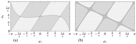
Figure 3: Shielding (light grey), amplification (medium grey) and neutral (dark grey) regions created by a microcrack and a rigid line inclusion arranged as shown in Fig. 2a. The diagrams are for a weak interface between two identical materials, $\eta=0$, and symmetrical loading, $b=0$. The position of the microcrack is characterised by the angles $\varphi_{1}$ and $\alpha_{1}$, whereas the position of the rigid line inclusion is determined by conditions (67). The dark grey region corresponds to neutral configurations, that is configurations for which the perturbation is negligibly small (within the accuracy $\delta=10^{-6}$). Figure (a): load is applied close to the crack tip, $a=3$. Figure (b): load is applied at a large distance from the crack tip, $a=100$.

In Fig. 4, we analyse the effect of the asymmetry of loading for the same configuration as in Fig. 3. The diagrams correspond to a three-point loading, characterised by the parameters $a$ and $b$, as shown in Fig. 2. The definition and range of the angles $\alpha_{1}$ and $\varphi_{1}$ are the same as in Fig. 3 ($-\pi<\varphi_{1}<\pi$, $0<\alpha_{1}<\pi$). We consider four values of the parameter $a$, namely $a=3,6,10,100$, from left to right. This allows us to trace different situations corresponding to the increasing distance of the loading from the crack tip (keeping $b$ fixed). The asymmetry of loading is measured by the parameter $b$, which increases from the upper part (symmetrical loading $b=0$) to the lower part ($b=0.99a$) of the figure.

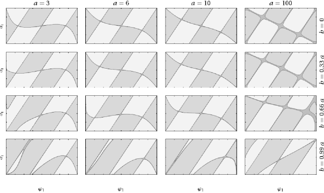
Figure 4: Shielding (light grey), amplification (medium grey) and neutral (dark grey) regions created by a microcrack and a rigid line inclusion arranged as shown in Fig. 2a. The diagrams are for a weak interface between two identical materials, $\eta=0$, and three-point loading, characterised by parameters $a$ and $b$. From left to right the distance $a$ of loading from the crack tip increases from $3$ to $100$. From up to bottom the asymmetry $b$ of loading increases from $0$ to $0.99a$.

From the results presented in Fig. 4, the following conclusions can be drawn. First, the neutral region (shadowed dark grey) enlarges when moving from the diagrams on the left to those on the right. This finding, already evident in Fig. 3 where only the values $a=3$ and $a=100$ were considered with $b=0$, confirms the validity of the simplified formulae (61) and (62), established in the literature (Gong, 1995). Secondly, it is clear that the asymmetry of loading plays an important role. Indeed, even for $a=100$ and $b=0.33a$, or $b=0.66a$, when the nearest point force is still well separated from the crack tip, the shielding–amplification diagrams are essentially different from those of the symmetrical case ($b=0$). Thirdly, since the distance of the loading from the crack tip is measured by $a-b$, the neutral region shrinks by increasing the asymmetry $b$ at fixed $a$ (thus moving from the diagrams on the upper part to those on the lower part).

In Fig. 5 and Fig. 6, we show the influence of the inhomogeneity on the shielding and amplification effects. For this purpose, we consider the aforementioned three-point loading for the case of a bimaterial plane with contrast parameter $\eta=0.67$ (diagrams of Fig. 5) and $\eta=-0.67$ (diagrams of Fig. 6). All other parameters ($a,b,\alpha_{1}$ and $\varphi_{1}$) are defined in the same manner as above.

Figure 5: Shielding (light grey), amplification (medium grey) and neutral (dark grey) regions created by a microcrack and a rigid line inclusion arranged as shown in Fig. 2a. The diagrams are for a bimaterial solid with $\eta=0.67$, and three-point loading, characterised by parameters $a$ and $b$. From left to right the distance $a$ of loading from the crack tip increases from $3$ to $100$. From up to bottom the asymmetry $b$ of loading increases from $0$ to $0.99a$.

Figure 6: Shielding (light grey), amplification (medium grey) and neutral (dark grey) regions created by a microcrack and a rigid line inclusion arranged as shown in Fig. 2a. The diagrams are for a bimaterial solid with $\eta=-0.67$, and three-point loading, characterised by parameters $a$ and $b$. From left to right the distance $a$ of loading from the crack tip increases from $3$ to $100$. From up to bottom the asymmetry $b$ of loading increases from $0$ to $0.99a$.

The influence of the inhomogeneity is clearly observable only for a highly pronounced non-symmetrical loading which is applied close to the crack tip. Furthermore, the shielding and amplification effects are more pronounced when the defects are located in the softer material (upper half-plane, $0<\varphi_{1}<\pi$, in Fig. 5; lower half-plane, $-\pi<\varphi_{1}<0$, in Fig. 6).

Finally, we comment on the arrangement (b), see Fig. 2b. This configuration turns out to be neutral for any symmetrical loading, independently of the distance $a$ from the crack tip, and the diagrams are very similar regardless of the bimaterial parameter $\eta$. For this reason, we present in Fig. 7 results only for the case of asymmetrical loading, $b\neq 0$, and weak interface between two identical materials, $\eta=0$.

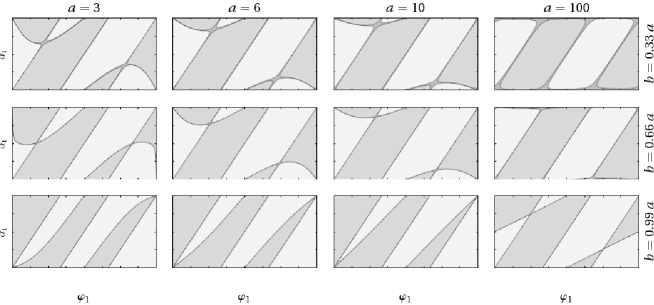
Figure 7: Shielding (light grey), amplification (medium grey) and neutral (dark grey) regions created by a microcrack and a rigid line inclusion arranged as shown in Fig. 2b. The diagrams are for a weak interface between two identical materials, $\eta=0$, and three-point loading, characterised by parameters $a$ and $b$. From left to right the distance $a$ of loading from the crack tip increases from $3$ to $100$. From up to bottom the asymmetry $b$ of loading increases from $0.33a$ to $0.99a$..

It follows from Fig. 7 that the neutrality property of arrangement (b) is broken by the asymmetry of loading and thus amplification–shielding regions appear for $b\neq 0$. Moreover, the influence of asymmetry is not only quantitative but also qualitative, since the diagrams are completely different for different values of $b$. This emphasises the importance of the skew-symmetric weight functions (Piccolroaz et al., 2009) which are used to evaluate the contribution of the skew-symmetric load.

4.2 Crack propagation and arrest

In this section we discuss the influence of small defects on the crack propagation, in particular on the crack “acceleration” and arrest. Given a configuration of defects and position of the crack tip with respect to the defects, the formula (59) allows for the computation of the incremental crack advance $\phi$. It is possible then to update the configuration with the new position of the crack tip with respect to the defects and recompute the incremental crack advance in the new configuration, following an iterative procedure. The crack “accelerates” when the increment $\phi$ is increasing and “decelerates” in the opposite case. The total crack elongation is computed as

$$x(N)=\sum_{i=0}^{N}\phi_{i},$$ (69)

where $N$ is the number of iterations.

In Fig. 8 we show the numerical results for the case of two defects (a microcrack and a rigid line inclusion) arranged as shown in Fig. 2a. The body is assumed homogeneous $\eta=0$ and the loading is symmetric $b=0$. The initial position of the microcrack relative to the main crack tip is characterised by the values $d_{1}=1$, $\varphi_{1}=\pi/8$. Five cases of angular orientation of the microcrack are considered, namely $\alpha_{1}=0,\pi/8,\pi/4,3\pi/8,\pi/2$, and denoted by labels from 1 to 5, see Fig. 8d. The initial position and the inclination of the rigid line inclusion is determined by conditions (67).

Fig. 8a shows the crack elongation $x$ as a function of the number of iterations. For all cases, we may observe crack acceleration followed by a rapid deceleration and arrest, see Fig. 8b. The crack arrests when a neutral configuration is reached at that particular position of the crack tip.. The total elongation at arrest is different for different cases. In the case denoted by 5, the crack advance is initially very slow, because the initial configuration is close to the border of the neutral region (dark grey region in Fig. 8d), but the crack reaches the largest elongation at arrest. The incremental crack advance $\phi$ is plotted against the crack elongation $x$ in Fig. 8c.

Figure 8: Acceleration and arrest of the main crack along a weak interface between two identical materials, produced by a microcrack and a rigid line inclusion arranged as in Fig. 2a. The initial position of the microcrack relative to the crack tip is characterised by the values $d_{1}=1$, $\varphi_{1}=\pi/8$. Five cases of angular orientation of the microcrack are considered, namely $\alpha_{1}=0,\pi/8,\pi/4,3\pi/8,\pi/2$, and denoted by labels from 1 to 5. The initial position and the inclination of the rigid line inclusion is determined by conditions (67). The crack elongation, denoted by $x$, is assumed equal to 0 in the initial configuration. Figure (a): crack elongation $x$ vs. number of iterations. Figure (b): increment $\phi$ vs. number of iterations. Figure (c): increment $\phi$ vs. crack elongation $x$. Figure (d): initial configurations are indicated by spots in the shielding–amplification diagram.

In Fig. 9 we consider the same situation as in Fig. 8, however now the initial position of the microcrack relative to the main crack tip is characterised by the values $d_{1}=1$, $\varphi_{1}=7\pi/8$, and four angular orientation are considered, $\alpha_{1}=3\pi/8,\pi/2,5\pi/8,3\pi/4$, see Fig. 9d. We may observe a crack acceleration followed by a slow deceleration until a steady-state propagation is reached. In fact, as the crack is propagating and the angle $\varphi_{1}$ is increasing (up to the maximum value $\pi$), the corresponding configuration will always remain in the amplification region, see Fig. 9d.

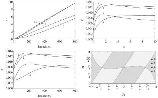
Figure 9: Initial acceleration followed by steady-state propagation of the main crack along a weak interface between two identical materials, produced by a microcrack and a rigid line inclusion arranged as in Fig. 2a. The initial position of the microcrack relative to the crack tip is characterised by the values $d_{1}=1$, $\varphi_{1}=7\pi/8$. Four cases of angular orientation of the microcrack are considered, namely $\alpha_{1}=3\pi/8,\pi/2,5\pi/8,3\pi/4$, and denoted by labels from 1 to 4. The initial position and the inclination of the rigid line inclusion is determined by conditions (67). The crack elongation, denoted by $x$, is assumed equal to 0 in the initial configuration. Figure (a): crack elongation $x$ vs. number of iterations. Figure (b): increment $\phi$ vs. number of iterations. Figure (c): increment $\phi$ vs. crack elongation $x$. Figure (d): initial configurations are indicated by spots in the shielding–amplification diagram.

5 Conclusions

In the present paper we show that the new weight functions for a bimaterial plane constructed in Piccolroaz et al. (2009) together with the dipole matrix approach provide an efficient tool in analysis of perturbation problems arising from the interaction of an interfacial crack with small defects, including elastic inclusions, microcracks, rigid line inclusions, and line defects with imperfect bonding. We also show that the skew-symmetric weight functions play a crucial role as they permit to evaluate the contribution of the skew-symmetric load applied along the crack faces.

We illustrate the method with a number of applications, ranging from the analysis of shielding–amplification effects of the defects on the crack-tip fields to the perturbation modelling of the quasi-static interface crack propagation. The influence of asymmetry and position of the loading with respect to the crack tip is discussed and quantified.

As a final remark, we note that the method can be extended to the case when the number of defects becomes increasingly high (clouds of defects). However, this requires additional accurate treatment of the interaction between defects and it is beyond the scope of the present paper.

Acknowledgement. This research was supported by the Research-In-Groups (RiGs) programme of the International Centre for Mathematical Sciences, Edinburgh, Scotland. In addition, A.P. and G.M. gratefully acknowledge the support from the European Union Seventh Framework Programme under contract numbers PIEF-GA-2009-252857 and PIAP-GA-2009-251475, respectively.

Appendix A APPENDIX

A.1 The dipole matrix for an elastic elliptic inclusion in antiplane shear

Although the general problem of an elliptic inclusion in an infinite medium subject to remote uniform stress has been known since the mid of the last century (Donnell, 1941; Hardiman, 1954), the dipole matrix in the case of antiplane shear is practically impossible to find in the existing literature. For this reason, we have decided to present here not only the matrix but also in brief its derivation.

We consider an elastic elliptic inclusion $g$, with shear modulus $\mu_{0}$, embedded in an infinite body with shear modulus $\mu$, undergoing antiplane shear deformation. The boundary of the inclusion is denoted by $\partial g=\{(x,y):x^{2}/a^{2}+y^{2}/b^{2}=1\}$.

The problem is formulated as follows:

$$\Delta u=0\quad\text{in}\quad\mathbb{R}^{2}\setminus\overline{g},$$

$$\Delta u_{0}=0\quad\text{in}\quad g,$$

$$u=u_{0},\quad\mu\frac{\partial u}{\partial n}=\mu_{0}\frac{\partial u_{0}}{\partial n}\quad\text{on}\quad\partial g,$$

$$u=B_{R}x-B_{I}y+O(1)\quad\text{as}\quad r=\sqrt{x^{2}+y^{2}}\to\infty,$$ (A.1)

where $u_{0}$ and $u$ are the displacements in the interior and exterior of the inclusion, respectively, $n$ is an outward unit normal on $\partial g$ and $B_{R}$, $B_{I}$ are known constants.

The displacement in the inclusion is linear (Horgan, 1995; Ru and Schiavone, 1996), so that

$$u_{0}=A_{R}x-A_{I}y\quad\text{in}\quad g.$$ (A.2)

Our objective is to compute the next term in the asymptotic of the displacement field at infinity, eq. (A.1), which will be provide us with the required dipole matrix. To this purpose we will use the theory of analytic functions. Thus, we write $u_{0}(x,y)=\mathop{\mathrm{Re}}U^{0}(z)=U^{0}_{R}(z)$ and $u(x,y)=\mathop{\mathrm{Re}}U(z)=U_{R}(z)$, where $U^{0}=Az$ is a linear function in $g$ and $U$ is an analytic function in $\Omega\setminus\overline{g}$ satisfying the following conditions

$$U=Bz+\frac{D_{1}}{z}+O(|z|^{-2}),\quad B=B_{R}+iB_{I},\quad D=D_{R}+iD_{I},\quad z\to\infty,$$

$$U^{0}_{R}-U_{R}=0,\quad\mu_{0}U^{0}_{I}-\mu U_{I}=0\quad\text{on}\quad\partial g.$$ (A.3)

Note that, in order to find the dipole matrix, we do not need the complete solution but only the constant $D_{1}$. Furthermore, we introduce the conformal mapping

$$z=c\left(\zeta+\frac{\lambda}{\zeta}\right),\quad c>0,\quad 0<\lambda<1,$$

which maps the ellipse $\partial g$ in the $z$-plane onto the unit circle in the $\zeta$-plane. The segment $d$ connecting the foci of the ellipse is mapped onto the circle $|\zeta|=\sqrt{\lambda}$, so that the region $g\setminus d$ is transformed into the ring $\sqrt{\lambda}<|\zeta|<1$.

We seek for the solution in the transformed coordinates in the form

$$U^{0}=Ac(\zeta+\lambda/\zeta),\quad U=\beta\zeta+\gamma_{1}/\zeta.$$ (A.4)

Such a solution exists with constants $\beta$ and $\gamma_{1}$ satisfying the following conditions

$$\gamma_{1R}=\beta_{R}\frac{\mu(1+\lambda)-\mu_{0}(1-\lambda)}{\mu(1+\lambda)+\mu_{0}(1-\lambda)},\quad\gamma_{1I}=-\beta_{I}\frac{\mu(1-\lambda)-\mu_{0}(1+\lambda)}{\mu(1-\lambda)+\mu_{0}(1+\lambda)}.$$

Going back to the original coordinates, from the asymptotic expansion $\zeta=z/c-c\lambda/z+O(|z|^{-3})$, $z\to\infty$, we get

$$\beta=cB,\quad D_{1}=\gamma_{1}c-\beta\lambda c.$$

As a result, we obtain the required two terms asymptotic of the displacement at infinity in the form

$$u=B_{R}x-B_{I}y-\frac{1}{2\pi}\{B_{R},-B_{I}\}\cdot\mbox{\boldmath$P$}\,\frac{\{x,y\}}{x^{2}+y^{2}}+O(r^{-2}),\quad\text{as}\quad r\to\infty,$$ (A.5)

where, taking into account that $c=(a+b)/2$ and $\lambda=(a-b)/(a+b)$, the dipole matrix $P$ is given by

$$\mbox{\boldmath$P$}=-\pi ab(a+b)\left[\begin{array}[]{ll}\displaystyle\frac{\mu-\mu_{0}}{\mu a+\mu_{0}b}&0\\[8.53581pt] 0&\displaystyle\frac{\mu-\mu_{0}}{\mu_{0}a+\mu b}\end{array}\right].$$ (A.6)

We obtain the solution we need in Sec. 3.1.1 by defining new functions $\tilde{u}=u-B_{R}x+B_{I}y$ and $\tilde{u}_{0}=u_{0}-B_{R}x+B_{I}y$. Then $\tilde{u}$ and $\tilde{u}_{0}$ satisfy a BVP similar to (A.1), in which the condition at infinity is replaced by $\tilde{u}\to 0$ as $r\to\infty$, and the ideal transmission conditions are replaced by imperfect transmission conditions as follows

$$\tilde{u}=\tilde{u}_{0},\quad\mu\frac{\partial\tilde{u}}{\partial n}-\mu_{0}\frac{\partial\tilde{u}_{0}}{\partial n}=-(\mu-\mu_{0})\mbox{\boldmath$n$}\cdot\{B_{R},-B_{I}\}\quad\text{on}\quad\partial g.$$

Appendix B Asymptotics at infinity for a movable rigid line inclusion

One can find, as a particular case from Muskhelishvili (2008), a solution $U$ for analytic function in the complex plane with given conditions along the symmetric segment of the length $2a$ situated along the real $x$-axis: $U^{+}=F(x)$, $U^{-}=F(x)$. The bounded solution for this problem reads

$$U(z)=\frac{\sqrt{R(z)}}{\pi i}\int_{-a}^{a}\frac{F(t)dt}{\sqrt{R(t)}(t-z)},$$ (B.7)

where $z=x+iy$, and $R(z)=z^{2}-a^{2}$. This solution vanishes at infinity if the following condition is satisfied

$$\int_{-a}^{a}\frac{F(t)}{\sqrt{-R(t)}}dt=0.$$ (B.8)

It is clear from (38) that this condition is satisfied, since for a rigid line inclusion $F(t)=Bt$, where $B=-\nabla_{\mbox{\boldmath$x$}}u^{(0)}|_{\mbox{\boldmath$Y$}_{3}}\cdot\mbox{\boldmath$\Phi$}^{T}(\alpha_{3})\mbox{\boldmath$e$}_{1}$, with $\Phi$ being the rotation matrix and $\mbox{\boldmath$e$}_{1}$ the unit vector along the $x$-axis. The asymptotics at infinity for this function takes the form

$$U(z)=\frac{Ba^{2}}{2z}+O(z^{-3}),\quad\text{as}\quad z\to\infty.$$ (B.9)

Thus, the boundary layer solution for a rigid line inclusion in the coordinate system $\mbox{\boldmath$\xi$}_{3}$ is given by a formula similar to (27) with $\mbox{\boldmath$\mathcal{M}$}_{1}$ replaced by (39).

References

• [1] Antipov, Y.A., Avila-Pozos, O., Kolaczkowski, S.T., Movchan, A.B., Mathematical model of delamination cracks on imperfect interfaces. Int. J. Solids Struct. 38, 6665–6697, (2001).
• [2] Benveniste, Y., Miloh, T., Imperfect soft and stiff interfaces in two-dimensional elasticity. Mech. Materials 33, 309–323, (2001).
• [3] Bigoni, D., Serkov, S.K., Movchan, A.B., Valentini, M., Asymptotic models of dilute composites with imperfectly bonded inclusions. Int. J. Solids Struct. 35, 3239–3258, (1998).
• [4] Donnell, L.H., Stress concentration due to elliptical discontinuities in plates under edge stresses. In Theodore von Karman Anniversary Volume, California Institute of Technology, 293–309, (1941).
• [5] Gong, S.X., On the main crack-microcrack interaction under Mode-III loading. Eng. Fract. Mech. 51, 753–762, (1995).
• [6] Gong, S.X., Horii, H., General solution to the problem of microcracks near the tip of a main crack. J. Mech. Phys. Solids 37, 27–46, (1989).
• [7] Hardiman, N. J., Elliptical elastic inclusion in an infinite elastic plane. Q. J. Mech. Appl. Math. 7, 226–230, 1954.
• [8] Hashin, Z., Thin interphase/imperfect interface in conduction. J. Appl. Phys. 89, 2261–2267, (2001).
• [9] Meguid, S.A., Gong, S.X., Gaultier, P.E., Main crack–microcrack interaction under Mode I, II, and III loading: shielding and amplification. Int. J. Mech. Sci. 33, 351–359, (1991).
• [10] Mishuris, G., Interface crack and nonideal interface concept (Mode III). Int. J. Fracture 107, 279–296, (2001).
• [11] Mishuris, G., Mode III interface crack lying at thin nonhomogeneous anisotropic interface. Asymptotics near the crack tip. In IUTAM Symposium on Asymptotics, Singularities and Homogenisation in Problems of Mechanics, A.B. Movchan (ed.), 251–260, (2003)
• [12] Movchan, A.B., Movchan, N.V., Mathematical modeling of solids with nonregular boundaries. CRC-Press, (1995).
• [13] Movchan, A.B., Movchan, N.V., Poulton, C.G., Asymptotic models of fields in dilute and denselly packed composites. Imperial College Press, (2002).
• [14] Muskhelishvili, N.I., Singular integral equations: boundary problems of function theory and their application to mathematical physics. Dover Edition, (2008).
• [15] Piccolroaz, A., Mishuris, G., Movchan, A.B., Symmetric and skew-symmetric weight functions in 2D perturbation models for semi-infinite interfacial cracks. J. Mech. Phys. Solids 57, 1657–1682, (2009).
• [16] Piccolroaz, A., Mishuris, G., Movchan, A.B., Perturbation of Mode III interfacial cracks. Int. J. Fracture 166, 51–41, (2010).
• [17] Romalis, N., Tamuzh, V., Propagation of a main crack in a body with distributed microcracks. Mech. Comp. Mater. 20, 35–43, (1984).
• [18] Tamuzs, V.P., Petrova, V.E., On macro–microdefect interaction. Int. Appl. Mech. 38, 1157–1177, (2002).
• [19] Tamuzs, V., Petrova, V., Romalis, N., Thermal fracture of macrocrack with closure as influenced by microcracks. Theor. Appl. Fract. Mech. 21, 207–218, (1994).
• [20] Tamuzs, V., Petrova, V., Romalis, N., Plane problem of macro–microcrack interaction taking account of crack closure. Eng. Fract. Mech. 55, 957–967, (1996).
• [21] Tamuzs, V., Romalis, N., Petrova, V., Influence of microcracks on thermal fracture of macrocrack. Theor. Appl. Fract. Mech. 19, 207–225, (1993).
• [22] Valentini, M., Serkov, S.K., Bigoni, D., Movchan, A.B., Crack propagation in a brittle elastic material with defects. ASME J. Appl. Mech. 66, 79–86, (1999).