Competing epidemics on complex networks

Abstract

Human diseases spread over networks of contacts between individuals and a substantial body of recent research has focused on the dynamics of the spreading process. Here we examine a model of two competing diseases spreading over the same network at the same time, where infection with either disease gives an individual subsequent immunity to both. Using a combination of analytic and numerical methods, we derive the phase diagram of the system and estimates of the expected final numbers of individuals infected with each disease. The system shows an unusual dynamical transition between dominance of one disease and dominance of the other as a function of their relative rates of growth. Close to this transition the final outcomes show strong dependence on stochastic fluctuations in the early stages of growth, dependence that decreases with increasing network size, but does so sufficiently slowly as still to be easily visible in systems with millions or billions of individuals. In most regions of the phase diagram we find that one disease eventually dominates while the other reaches only a vanishing fraction of the network, but the system also displays a significant coexistence regime in which both diseases reach epidemic proportions and infect an extensive fraction of the network.

I Introduction

Diseases spread over networks of contacts between individuals, and a full understanding of their nature and behavior requires an understanding of the relevant network structure and the effects that structure has on the spreading process. Traditional theories of disease propagation largely ignore network effects AM91 ; Hethcote00 , but there has been a significant volume of research in recent years aimed at building an understanding of the role that networks play Keeling01 ; Liljeros01 ; PV01a ; Newman02c ; Bansal20071 ; Kenah2011 . Network epidemiology ideas have also been applied to cultural transmission processes, such as the spread of ideas, rumors, fashions, or opinions, which may occur by mechanisms qualitatively similar in some respects to the spread of biological disease DW04 .

One of the most fundamental and important theoretical models of disease spreading is the susceptible-infected-recovered (SIR) model, in which initially susceptible individuals catch the disease of interest from infected individuals, becoming infected themselves and possibly passing the disease to others, before recovering and acquiring permanent immunity so that each individual catches the disease at most once. As well as being a reasonably accurate, if simplified, representation of the dynamics of many real-world diseases, the SIR model is important to network epidemiology from a theoretical viewpoint because it is closely related to bond percolation on a given contact network Mollison77 ; Grassberger83 ; Sander02 ; Newman02c ; Kenah2011 . The mapping is a straightforward one: edges in the network are occupied with independent probability $T$, equal to the time-integrated probability that a neighbor of an infected individual will become infected. The value of $T$ is a property both of the disease and of individuals’ behavior, and is called the transmissibility or infectivity. The occupied edges of the network form connected percolation clusters and the members of a cluster represent the set of vertices that will become infected in the limit of long time if any vertex in the cluster is initially infected. In general the clusters are small for low values of the transmissibility, consisting of only few vertices each, but as the transmissibility increases they become larger and eventually an extensive giant cluster forms, corresponding to a potential epidemic outbreak of the disease in which an non-negligible fraction of the population becomes infected. The point at which the giant cluster forms is a continuous phase transition and is referred to in the epidemiology literature as the epidemic threshold.

In this paper we study the behavior of two SIR-type diseases competing for the same population of hosts and spreading over the same contact network. In some cases a pair of diseases—or two strains of the same disease, such as two strains of influenza—spread through the same population and interact through cross-immunity: infection with and recovery from either strain imparts subsequent immunity to both so that each individual can catch at most one of the two strains. The question we address is whether and how far the two strains will spread under such circumstances, as a function of parameters such as transmissibility and network structure.

A simple case of this problem was studied previously by Newman Newman05c using the mapping to bond percolation described above. In that work it was assumed that the spread of one disease begins only after the other has entirely run its course. The first disease can then be regarded as effectively removing from the population all individuals it infects, leaving a pared-down remnant of the original network, referred to as the residual network, for the second disease to spread on. If the first disease spreads too readily and consumes too large a portion of the network, then the residual network will be too sparse to support the spread of the second disease. Thus there is an upper limit on the transmissibility of the first disease if the second is to spread, which was dubbed the coexistence threshold in Ref. Newman05c .

In this paper, we study the more general—and more realistic—case in which the two diseases spread concurrently. Although this appears to be a harder problem it turns out, as we will show, that many of the results of the earlier analysis can be applied or adapted to the more general situation. (A different generalization to the case in which one disease confers only partial immunity to the other, has been studied by Funk and Jansen Funk2010 . The case of full cross-immunity for concurrent diseases following a susceptible-infected-susceptible (SIS) dynamics has also been studied Ahn2006 , but the results are not directly applicable to the case we study because the SIS model does not map to bond percolation.)

When studying diseases spreading at well separated times, the precise dynamics of the diseases is not important for predicting the final outbreak sizes. The mapping to percolation tells us everything we need to know and details like whether one disease spreads faster than the other have no effect. When considering the concurrent spread of diseases, however, such details are important and we must specify what dynamics we are considering. In this paper we adopt one of the simplest and best-known of dynamical frameworks for SIR diseases, the Reed–Frost model. This model uses a discrete time-step for its evolution and on each step susceptible individuals have a fixed probability, equal to the transmissibility $T$, of being infected by each of their infected network neighbors, so that a susceptible individual with $k$ infected neighbors remains susceptible with probability $(1-T)^{k}$. Infected individuals remain infected for exactly one time-step and then recover, becoming immune and remaining in the immune state indefinitely thereafter. Thus the model has just two parameters, the length of the time-step and the transmissibility. (The other common choice for SIR dynamics, the Kermack–McKendrick model, uses continuous time and stochastically constant rates of infection and recovery, but again has just two parameters, equal to the two rates. The Kermack–McKendrick model can also be mapped to a bond percolation process, but on a directed, rather than undirected, network, which makes its analysis less transparent, and it is in part for this reason that we use the Reed–Frost model in this paper.)

In our studies we make use of a two-disease generalization of the Reed–Frost model as follows. The two diseases, which we label red and blue, each start from a single, randomly chosen, infected vertex. In the simplest case the two diseases are assumed to start at the same instant, although we will relax this condition later. The diseases have transmissibilities $T_{r}$ and $T_{b}$, for red and blue respectively. We also allow their time-steps to be different, so that one spreads on a faster clock than the other. Only the ratio of the time-steps is important for our results, not the overall time-scale, so we fix the time-step for the blue disease to be 1 and vary the time-step for the red disease, which we denote $\alpha$. Without loss of generality we assume that $0\leq\alpha\leq 1$, meaning that red always spreads faster than (or at the same speed as) blue.

Thus there are three parameters in our two-disease Reed–Frost model, $T_{r}$, $T_{b}$, and $\alpha$, as opposed to two in the one-disease version. Despite its simplicity, we will see that this model displays some complex and interesting behaviors.

II Principal results

The behavior of the system we study is, as we have said, quite complex, so we begin in this section with a nontechnical summary. Detailed arguments and numerical results are given in the following sections.

Initially we consider the results in the limit of large network size, for which the behavior of the system is relatively simple. As we will show, however, networks must, in some parameter ranges, be very large indeed to be considered “large” in this sense, and real contact networks—even networks of billions of people—are not large enough. Thus finite-size effects can be important under real-world conditions, and so we give an analysis of these also.

Consider then the behavior of the system on a contact network of $n$ vertices, in the limit of large $n$. In order to take the limit we need to specify how our contact network is defined for given $n$. The analytic and numerical results in this paper are all calculated using the so-called configuration model MR95 ; NSW01 , i.e., a random graph with a specified degree distribution, and the limit of large network size is taken as the limit of this model with the degree distribution held fixed note1 . Qualitatively, the results we report should apply to other networks as well, subject to some relatively mild conditions, but our quantitative results are all for the configuration model.

For given values of the three parameters $T_{r}$, $T_{b}$, and $\alpha$, we consider the fate of our two diseases as they each spread from a single randomly chosen initial disease carrier. Let us suppose that the epidemic threshold for our network—the position of the percolation transition, as discussed in the introduction—falls at a critical bond probability $\phi_{c}$. For instance, on configuration model networks it is known that

$$\phi_{c}={\langle k\rangle\over\langle k^{2}\rangle-\langle k\rangle},$$ (1)

where $\langle k\rangle$ and $\langle k^{2}\rangle$ represent the mean and mean-square degrees respectively CEBH00 ; CNSW00 . If the transmissibility of either of our diseases falls below this value the disease will not spread, reaching only $\mathrm{O}(1)$ vertices before dying out, in which case that disease can be ignored and the outcome for the other disease is given by standard single-disease results. For nontrivial results, therefore, we require $T_{r},T_{b}>\phi_{c}$.

Even for transmissibility above the epidemic threshold it is not guaranteed that a disease will spread. A disease starting from a single initial carrier can still die out, either because it starts in a small component of the network (not the giant component) or just because of stochastic fluctuations in the spreading process. Again, however, this gives trivial behavior, and so we limit our discussion to cases in which both diseases “take off,” meaning that both would, in the absence of the other disease, ultimately reach epidemic proportions, infecting an extensive fraction of the network in the limit of large size.

With these assumptions, both diseases spread exponentially at first: each is surrounded by a sea of susceptible individuals to infect—a naive population in the epidemiology jargon—and on an arbitrarily large network the two diseases start arbitrarily far apart and hence do not initially interfere with one another. The rate of exponential growth for the blue disease depends on $T_{b}$ and for the red disease on $T_{r}$ and $\alpha$. We will shortly calculate what these rates are, but for the moment suppose that we know the rates and that the ratio of the rate for red to the rate for blue is $\beta$. Then on average the number of individuals infected by blue goes as $N_{b}=\mathrm{e}^{rt}$ for some rate $r$ (with the overall multiplier fixed by the condition that $N_{b}=1$ at $t=0$) and the number infected by red goes as $N_{r}=\mathrm{e}^{\beta rt}=N_{b}^{\beta}$.

Now suppose that $\beta<1$, meaning that red grows slower and blue grows faster, and let us wait a certain amount of time until blue grows to fill $\mathrm{O}(n)$ vertices, meaning that $N_{b}=cn$ for some small constant $c$. In the same amount of time red infects $N_{r}=N_{b}^{\beta}=(cn)^{\beta}$ vertices, which is a fraction $(cn)^{\beta}/n=c^{\beta}/n^{1-\beta}$ of the entire network, i.e., a vanishing fraction in the limit of large $n$ since $\beta<1$. Thus, as far as the blue disease is concerned, red is irrelevant—cross-immunity of individuals previously infected with the red disease is a negligible impediment to blue’s spread, and blue’s dynamics will be the same as if it were the only disease. We can make a similar argument for the case where $\beta>1$ and red grows faster, showing that in the time red takes to reach $\mathrm{O}(n)$ vertices blue reaches only $\mathrm{O}(n^{1/\beta})$, or a fraction $\mathrm{O}(1/n^{1-1/\beta})$, which is again negligible in the limit of large $n$.

This insight is important because it allows us to treat our concurrent diseases as if they were in fact spreading non-concurrently, one after the other. The faster disease spreads to the entire network, infecting essentially everyone it was going to infect, before the slower disease rises beyond the level of insignificance. This means that, in the limit of large $n$, the eventual outcome for the two diseases can be predicted using static percolation arguments of the type employed for time-separated diseases in the work of Newman Newman05c discussed in the introduction.

The value $\beta=1$ at which the growth rates of the two diseases are equal forms a surface in the three-dimensional parameter space $(T_{r},T_{b},\alpha)$ of the model. On one side of this surface the blue disease grows faster and is equivalent to the first disease in the time-separated picture of Ref. Newman05c , while the red disease plays the role of the second disease. On the other side of the surface the roles are reversed.

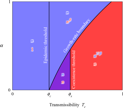
Figure 1: A two-dimensional slice through the phase diagram of the system, with $T_{b}$ held constant while $T_{r}$ and $\alpha$ vary. The area colors represent the dominant disease in each phase, while the colored symbols give the leading-order scaling of the expected number of individuals infected with each disease.

Figure 1 shows a two-dimensional slice of the parameter space for fixed $T_{b}$ and varying values of $T_{r}$ and $\alpha$. The surface $\beta=1$ is represented by the diagonal curve, colored blue on one side and red on the other to represent the dominant disease. If we are in the regime $\beta>1$, which is to the right of the curve, then red will always produce an epidemic. When red has run its course and finished spreading (but blue has still reached only a vanishing fraction of the network), it leaves behind it a residual network, as described earlier, and blue will spread further only if that residual network is sufficiently dense that the threshold for bond percolation on it falls below $T_{b}$. Just as before, this places an upper limit on the value of $T_{r}$ if both diseases are to spread, which we call the coexistence threshold and denote $\phi_{x}$. If $T_{r}<\phi_{x}$ then blue can spread and cause its own epidemic; if not, then blue only ever infects $\mathrm{O}(n^{1/\beta})$ vertices. The value $T_{r}=\phi_{x}$ constitutes another surface in the parameter space, which appears as a vertical straight line in Fig. 1, separating the coexistence regime (colored purple) from the regime where there is only one epidemic (red). Note that the value of $\phi_{x}$ depends on the transmissibility $T_{b}$ of the blue disease—a more virulent blue disease may spread on a residual network were a less virulent one would fail—so the position of the vertical line will shift as we take different slices through the parameter space note2 .

One might imagine that one would see a similar behavior on the other (left-hand) side of the curve in Fig. 1. On this side the blue disease spreads faster and will always cause an epidemic, but if its transmissibility is sufficiently low, one might argue, then it could leave behind a residual network dense enough to allow the red disease to subsequently spread and also cause an epidemic. It turns out, however, that this does not occur. As we will show, a necessary condition for coexistence of the slower red disease in this case is that $T_{r}>T_{b}$. However, given that $\alpha\leq 1$, it turns out that we also require $T_{b}>T_{r}$ if blue is to be the faster disease in the first place, and hence we have a contradiction and coexistence is not possible. Thus there is no coexistence region to the left of the curve.

Figure 1 is completed by a third line, again vertical, representing the point at which $T_{r}$ falls below the percolation threshold $\phi_{c}$. To the left of this line, the red disease does not cause an epidemic under any circumstances, infecting only $\mathrm{O}(1)$ individuals.

The complete figure constitutes a phase diagram for this system and has four regions, in one of which we have coexistence of the two diseases, while in each of the others one disease dominates and the other disease reaches only a vanishing fraction of the network. Note that the percolation and coexistence thresholds, which were identified previously Newman05c , correspond to continuous phase transitions in the sizes of the epidemics, but the curved $\beta=1$ boundary marks a different kind of transition at which the sizes jump discontinuously. This transition, which is a purely dynamical phenomenon driven by the differing exponential growth rates of the diseases, was not present in previous studies.

An interesting feature of the phase diagram is that there can be a maximum value of $\alpha$ above which coexistence does not occur—note that the purple coexistence region extends only up to a certain value of $\alpha$ and not beyond. Thus, for instance, for a random graph with a Poisson degree distribution, it turns out that coexistence requires $\alpha\leq\frac{1}{2}$, meaning that the red disease must spread at least twice as fast as the blue disease.

While still treating the large-size limit, we can consider other variants of our model. In particular, the assumption that both diseases start spreading at the same moment is unrealistic and can be relaxed. In most real-world cases one disease (or one strain of disease) starts spreading before the other, which is equivalent to having both start at $t=0$ but having one disease start with more than one carrier while the other starts with just one. As long as the number of initial carriers for both diseases is constant, however, this makes no difference in the limit of large network size because the disease with the larger exponential growth rate will always win in the end. Asymptotically, therefore, the phase diagram and other properties are unchanged.

The picture changes, however, when we consider a network of finite size. For diseases that start at the same moment we can make the same argument as before: in the time it takes for the faster-growing disease to spread to $\mathrm{O}(n)$ vertices the slower-growing one spreads to $\mathrm{O}(n^{\beta})$ or $\mathrm{O}(n^{1/\beta})$, as appropriate. Close to the $\beta=1$ boundary, however, $\mathrm{O}(n^{\beta})$ could be a large number, so there will be some rounding of the previously discontinuous transition as we cross the boundary. (In this sense the transition is unlike a traditional first-order phase transition, which remains discontinuous in a finite-sized system but shows fluctuations in its position. In the present model the position of the transition is unchanged but it is no longer discontinuous.) The other transitions, which are continuous phase transitions, will also show rounding, as is typical of such transitions in finite systems.

A more dramatic difference appears if, as above, we allow the diseases to start their spread at different times, or equivalently give one disease a larger number of initial carriers than the other. In particular, if we give a head start to the disease with the slower exponential growth rate then, depending on the size of that head start and the difference in rates, it is possible that the slower disease will, on the finite network, reach a significant fraction of the vertices in advance of the faster disease. The faster disease simply does not have enough time to overtake the slower one’s lead and exclude it from the network. In this case it is possible for the slower disease to actually exclude the faster one, imparting immunity upon a sufficiently large fraction of individuals as to prevent an epidemic of the faster disease, a complete reversal of the behavior in the infinite-size limit.

Suppose for example that the blue disease is faster, meaning that $\beta<1$. As before the blue disease starts with a single carrier at $t=0$ and the number grows as $N_{b}=\mathrm{e}^{rt}$ on average for some constant $r$. But let us now suppose that red has $A>1$ infected carriers at $t=0$, so that its number of cases is not $\mathrm{e}^{\beta rt}$ but $N_{r}=A\mathrm{e}^{\beta rt}=AN_{b}^{\beta}$. The faster blue disease will catch up to the slower red one at the point where $N_{b}=N_{r}$ or equivalently $N_{b}=AN_{b}^{\beta}$, which can be rearranged to give $N_{b}=A^{1/(1-\beta)}$. If blue is to catch up to red, this point must fall well before we reach the size $n$ of the entire network and the exponential growth of the diseases is exhausted. In other words, blue catches up only if

$$n\gg A^{1/(1-\beta)}.$$ (2)

We can make a similar argument if $\beta>1$ and red is the faster disease. The result is the same but with $\beta$ replaced by $1/\beta$.

But note that if the growth rates of the two diseases are similar, so that $\beta$ is close to 1, then the exponent in Eq. (2) becomes large, meaning that the network needs to be very large to prevent the slower disease from dominating. With $\beta=0.9$, for instance, and a modest value of $A=10$, we would need $n\gg 10^{10}$, which is several orders of magnitude larger than the population of the Earth. Thus the finite-size effects can be very much noticeable for populations of realistic sizes.

Moreover, we have throughout this argument ignored stochastic fluctuations in the growth process. In the early stages of development of an epidemic, when only a handful of individuals are infected, fluctuations can be large as a fraction of epidemic size—easily a factor of two or more—and this can either increase or decrease the lead that one disease has over another, or create a lead where none existed previously. Even if our two diseases start spreading at exactly the same moment, a lead gained by the slower disease, by virtue of chance fluctuations early in the process, can be enough, particularly when $\beta$ is close to 1, to allow it to dominate, or at least coexist with, the other disease, in defiance of the predictions of the infinite-$n$ theory. This behavior means that the outcome is broadly undetermined for random initial conditions on finite-sized networks within certain regions of the parameter space. (We note that this is quite different from the behavior of a single disease modeled with the SIR model, for which initial fluctuations have no effect whatsoever on the final number of individuals infected, assuming that the disease does not die out.)

On the other hand, as we will see, if we wait some time until one disease has grown to fill a small fraction of the network and the period of gross initial fluctuations has ended, then it is possible to predict the final outcome quite accurately from arguments such as those above. One would not be far off the mark if one where to assume the dynamics to be governed by a deterministic growth process after waiting a suitable initial period for the fluctuations to become small. In this regard, our results agree with recent work by Marceau et al. Marceau2011 , who consider a deterministic differential equation model of competing diseases and show that it is able to predict final outcomes with some accuracy, but only given an initial condition that specifies the fraction of individuals infected with each disease at a time after fluctuations have become negligible. Thus a deterministic approximation does seem to work in this regime, although it also misses some of the most interesting phenomena exhibited by the system.

In the following sections we discuss the results above in more detail, giving a combination of analytic derivations and numerical results to motivate our conclusions.

III Epidemic growth rates

Our first step in demonstrating the results summarized in Section II is to derive the exponential growth of each of the two diseases in the absence of the other. In the epidemiology literature the growth of diseases is usually parametrized by the basic reproductive ratio $R_{0}$, which is the average number of additional infections caused by a newly infected individual. Consider a vertex in our network model that is infected by a disease with transmissibility $T$ and suppose the vertex has $k$ network neighbors excluding the one that gave it the disease in the first place (which is obviously already infected)—$k$ is the so-called excess degree. At early times the neighbors will, with high probability, all be susceptible and each becomes infected with independent probability $T$, so that the expected number of infectees is $Tk$. The value of $R_{0}$ is the average of this quantity over the excess degree $k$.

Let $p_{k}$ be the degree distribution of the network, i.e., $p_{k}$ is the fraction of vertices with degree $k$. The excess degree, however, is distributed not according to this distribution, but according to its own excess degree distribution NSW01

$$q_{k}={(k+1)p_{k+1}\over\langle k\rangle},$$ (3)

where $\langle k\rangle=\sum_{k}kp_{k}$ is, as before, the mean degree in the network. Performing the average over the excess degree, the basic reproductive ratio is now given by

$$R_{0} =T\sum_{k=0}^{\infty}kq_{k}={T\over\langle k\rangle}\sum_{k=0}^{\infty}k(k-1)p_{k}$$

$$=T{\langle k^{2}\rangle-\langle k\rangle\over\langle k\rangle}.$$ (4)

The epidemic threshold, which separates the regime in which the disease dies out from the regime in which it grows exponentially, is the point at which $R_{0}=1$, or equivalently the point at which $T=\phi_{c}=\langle k\rangle/(\langle k^{2}\rangle-\langle k\rangle)$, as in Eq. (1).

In the Reed–Frost model in a naive population, each infected individual infects, on average, $R_{0}$ susceptibles on each time-step, then recovers and is no longer infectious. Thus $R_{0}$ is precisely the average factor by which the number of infected individuals changes on each step. If we define

$$R_{b}=T_{b}{\langle k^{2}\rangle-\langle k\rangle\over\langle k\rangle}={T_{b}\over\phi_{c}}$$ (5)

to be the reproductive number for the blue disease in our two-disease system, and recall that the blue disease by hypothesis executes exactly one time-step per unit time, then in a naive population the average number of individuals infected with the blue disease at early times $t$ is

$$N_{b}=R_{b}^{t}=\mathrm{e}^{t\ln R_{b}},$$ (6)

where the outbreak is assumed to start from a single infected carrier at $t=0$ note3 .

Similarly for the red disease we can define

$$R_{r}=T_{r}{\langle k^{2}\rangle-\langle k\rangle\over\langle k\rangle}={T_{r}\over\phi_{c}}.$$ (7)

But recall that the red disease executes one time-step every $\alpha$ units of time, which means that the average number of individuals infected with red at early times is

$$N_{r}=R_{r}^{t/\alpha}=\mathrm{e}^{(t/\alpha)\ln R_{r}}.$$ (8)

Thus both diseases display exponential growth but with different growth rates: $\ln R_{b}$ for blue and $\alpha^{-1}\ln R_{r}$ for red. Note that these rates are both positive provided both diseases are above the epidemic threshold, so that $R_{b},R_{r}>1$.

We define $\beta$ as before to be the ratio of the exponential growth rates of the two diseases:

$$\beta=\frac{\ln R_{r}}{\alpha\ln R_{b}}=\frac{\ln(T_{r}/\phi_{c})}{\alpha\ln(T_{b}/\phi_{c})},$$ (9)

which we can calculate explicitly given the values of $T_{b}$, $T_{r}$, $\alpha$, and the degree distribution of the network. Now, by the argument given in Section II, we can show that for a network of $n$ vertices with $n$ large, the faster-growing disease will fill a fraction $\mathrm{O}(n)$ of the network before the slower one has a chance to fill more than a vanishing fraction. Therefore the faster disease can be treated as if the slower one did not exist and the analysis for non-concurrent diseases, spreading one after another, applies. (As we pointed out in Section II, other behaviors are possible on finite networks, but for the moment let us focus on the large-$n$ limit.)

Equation (9) allows us to calculate the position of the diagonal curve in Fig. 1, which we call the growth-rate boundary, separating the region where the blue disease dominates from the region where the red one does. This boundary corresponds, as we have seen, to $\beta=1$, and hence is given by

$$\alpha={\ln(T_{r}/\phi_{c})\over\ln(T_{b}/\phi_{c})}.$$ (10)

Note that this implies that the boundary meets the $\alpha=0$ axis at the epidemic threshold $T_{r}=\phi_{c}$ for the red disease, as depicted in Fig. 1.

IV Percolation analysis

Given that the two diseases can be treated as being well separated in time, we can now apply a bond percolation analysis to derive a number of useful results concerning the transmissibilities and the positions of the various transitions depicted in the phase diagram of Fig. 1. Such an analysis was described previously in Ref. Newman05c , whose results we review and extend in this section.

Consider our two diseases spreading on a configuration model network with degree distribution $p_{k}$ and $n$ vertices, where $n$ is again large, and let us suppose, for the sake of argument, that the red disease has the faster rate of growth, so that it can be treated as running its course first, to be followed later by the blue disease. (The case where blue grows faster can be treated by similar arguments, but with the colors reversed.) We thus consider a bond percolation process on our network with bond occupation probability equal to the transmissibility $T_{r}$ of the red disease. The size of an epidemic outbreak of the disease, the number of people affected by the disease in the limit of long time, is then equal to the size of the giant percolation cluster, as described in the introduction.

Consider any vertex in the network and let $u$ be the probability that it is not connected to the giant cluster by a particular one of its edges. This can happen in either of two ways. First, the edge could be unoccupied, which occurs with probability $1-T_{r}$. Second, the edge could be occupied (probability $T_{r}$) but the vertex at its other end does not belong to the giant cluster. The latter happens if and only if none of that vertex’s other edges connect it to the giant cluster, which occurs with probability $u^{k}$, where $k$ is the number of other edges, the quantity we call the excess degree. Thus the total probability is $1-T_{r}+T_{r}u^{k}$. Now we average this expression over the distribution $q_{k}$ of the excess degree, Eq. (3), to get a complete expression for $u$ thus:

$$u=\sum_{k=0}^{\infty}q_{k}(1-T_{r}+T_{r}u^{k})=1-T_{r}+T_{r}F_{1}(u),$$ (11)

where $F_{1}(z)=\sum_{k}q_{k}z^{k}$ is the probability generating function for the excess degree distribution and we have made use of the normalization condition $\sum_{k}q_{k}=1$.

If we can solve Eq. (11) for $u$, we can use the result to calculate the size of the giant cluster. A randomly chosen vertex of (total) degree $k$ is not in the giant cluster if none of its edges connect it to that cluster, which happens with probability $u^{k}$ again. Now, however, $k$ is distributed according to the total degree distribution $p_{k}$, so the average probability of being outside the giant cluster is $\sum_{k}p_{k}u^{k}=F_{0}(u)$ and the probability of being in the giant cluster is

$$S=1-F_{0}(u),$$ (12)

where $F_{0}(z)=\sum_{k}p_{k}z^{k}$ is the generating function for the degree distribution. But this probability is also equal to the expected fraction of the network occupied by the giant cluster, and hence $S$ gives us the size of the giant cluster as a fraction of $n$.

The portion of the network not in the giant cluster, which may include more than one network component, is the portion we previously called the residual network. It is the portion not infected by the red disease and hence not immune to subsequent infection by the blue disease. To find out whether the blue disease will cause a second epidemic, and if so how many individuals it will infect, we must now perform a second bond percolation calculation on this residual network.

It is straightforward to show that the residual network itself constitutes another configuration model network, i.e., a random graph with a given degree distribution, but the degree distribution is different in general from that of the original network because in removing the vertices infected by the red disease we reduce the degrees of their uninfected neighbors. The degree distribution of the residual network cannot be expressed simply in closed form but, as shown in Newman05c , its generating function, which we denote $G_{0}(z)$, can:

$$G_{0}(z)=\frac{F_{0}\bigl{(}u+(z-1)F_{1}(u)\bigr{)}}{F_{0}(u)},$$ (13)

where $F_{0}$, $F_{1}$, and $u$ are defined as previously. Similarly, the generating function for the excess degree distribution on the residual network is

$$G_{1}(z)=\frac{F_{1}\bigl{(}u+(z-1)F_{1}(u)\bigr{)}}{F_{1}(u)}.$$ (14)

Given these expressions the percolation properties of the residual network are straightforward to calculate. Consider a bond percolation process on a configuration model having the degree distribution implied by Eqs. (13) and (14), with bond occupation probability $T_{b}$. We consider any vertex in the network and let $v$ be the probability that it is not connected to the giant cluster of the new percolation process by a particular one of its edges. Then, by the same argument as before, $v$ is a solution of

$$v=1-T_{b}+T_{b}G_{1}(v),$$ (15)

and the fraction $C$ of the residual network filled by the giant cluster is

$$C=1-G_{0}(v).$$ (16)

Since the residual network is itself a fraction $1-S$ of the original network, the giant cluster of the second percolation process fills a fraction $C(1-S)$ of the original $n$ vertices.

We can also calculate the positions of the epidemic thresholds for the two diseases. They are given by Eq. (1) with the degree averages calculated for the entire network or the residual network, as appropriate. Alternatively, the thresholds can be expressed in terms of the generating functions. The basic reproductive ratio is given by Eq. (4) to be

$$R_{r}=T_{r}\sum_{k=0}^{\infty}kq_{k}=T_{r}F_{1}^{\prime}(1),$$ (17)

where the prime indicates a derivative. The epidemic threshold corresponds to the point $R_{r}=1$, i.e., the point where $T_{r}$ is equal to $1/F_{1}^{\prime}(1)$. (It is straightforward to show that this gives the same result as Eq. (1).) Similarly the threshold for the blue disease on the residual network is

$$\phi_{b}={1\over G_{1}^{\prime}(1)}={1\over F_{1}^{\prime}(u)},$$ (18)

where we have used Eq. (14). Note that the value of $u$ depends on $T_{r}$ via Eq. (11) and hence so does the value of $\phi_{b}$. Thus Eq. (18) also implicitly defines the coexistence threshold $\phi_{x}$ as the value of $T_{r}$ at which $\phi_{b}=T_{b}$ and the blue disease fails to spread. That is, the coexistence threshold is the value $\phi_{x}$ such that $T_{b}=1/F_{1}^{\prime}(u)$ when $u$ is the solution of $u=1-\phi_{x}+\phi_{x}F_{1}(u)$. Rearranging both expressions, we could alternatively write

$$\phi_{x}={1-u\over 1-F_{1}(u)},$$ (19)

where $u$ satisfies $F_{1}^{\prime}(u)=1/T_{b}$.

In Newman05c it was shown always to be the case that $\phi_{b}>\phi_{c}$—the threshold for the second disease to spread is greater than the threshold for the first. However, a stronger result also holds, which will be important for our work: it turns out that $\phi_{b}$ must be greater also than $T_{r}$. To see this, we first rearrange Eq. (11) to give an expression for $T_{r}$ thus:

$$T_{r}={1-u\over 1-F_{1}(u)},$$ (20)

(which is similar to Eq. (19), except that $u$ may now take any value, where in (19) it takes the value that satisfies $F_{1}^{\prime}(u)=1/T_{b}$).

Recall that $u$ represents the probability that an edge connects to a vertex not in the giant cluster of the red disease, and this probability can only decrease (or stay the same) when $T_{r}$ increases, which implies that $\mathrm{d}T_{r}/\mathrm{d}u\leq 0$. Performing the derivative, we then find that $F_{1}(u)-1+(1-u)F_{1}^{\prime}(u)\leq 0$, and rearranging this expression we have

$$T_{r}={1-u\over 1-F_{1}(u)}\leq{1\over F_{1}^{\prime}(u)}=\phi_{b}.$$ (21)

Since $T_{b}>\phi_{b}$ for the second disease to spread, this result implies that $T_{b}>T_{r}$ also. Thus the second disease must have a higher transmissibility than the first for coexistence to occur. This means, for instance, that we cannot have coexistence of two diseases with the same transmissibility.

We can make similar arguments if the roles of red and blue diseases are reversed. If blue is the faster growing then it spreads first and red spreads subsequently over the residual network blue leaves behind. The same equations apply for the sizes of the epidemics and the thresholds, and we can show that $T_{r}>T_{b}$ is a necessary condition for red to spread extensively. In this regime, however, the quantity $\beta$, Eq. (9), is by definition less than unity and hence $\ln(T_{r}/\phi_{c})<\alpha\ln(T_{b}/\phi_{c})$. Rearranging, we then have

$$\ln T_{r}<\alpha\ln T_{b}+(1-\alpha)\ln\phi_{c}\leq\ln T_{b},$$ (22)

and hence $T_{r}<T_{b}$. Thus it is never the case in this regime that $T_{r}>T_{b}$ and so, as claimed in Section II, coexistence is not possible when blue is the faster growing disease.

Thus one is left with slightly contrary criteria for coexistence. On the one hand we must be in the regime where red is the faster growing disease, but on the other hand blue must have the higher probability of transmission. It is possible this type of behavior may not be common for real diseases—it seems reasonable that the disease with higher transmissibility would grow faster, not slower—and hence it may be that the conditions for coexistence of competing diseases in a single population are met rather rarely.

As a concrete example of the results of this section, consider a faster red disease and a slower blue one spreading on a network with the Poisson degree distribution $p_{k}=e^{-c}c^{k}/k!$. In this case $F_{0}(z)=F_{1}(z)=e^{c(z-1)}$—so the degree and excess degree distributions are the same—and $\phi_{c}=1/F_{1}^{\prime}(1)=1/c$. The coexistence threshold $\phi_{x}$ is then given by Eq. (19) where $u$ is the solution of $F_{1}^{\prime}(u)=1/T_{b}$, or

$$u=1-{1\over c}\ln cT_{b}.$$ (23)

Substituting this value into (19) gives

$$\phi_{x}={T_{b}\ln cT_{b}\over cT_{b}-1}.$$ (24)

We can also use the results of this section to find the maximum value of $\alpha$ beyond which coexistence does not occur. Referring to Fig. 1, we see that the maximum falls on the growth-rate boundary defined by Eq. (10), at the point where $T_{r}=\phi_{x}$. For the Poisson degree distribution above, for example, Eq. (10) becomes

$$\alpha={\ln cT_{r}\over\ln cT_{b}},$$ (25)

and substitution from Eq. (24) then gives

$$\alpha_{\textrm{max}}=1-{\ln(cT_{b}-1)-\ln\ln cT_{b}\over\ln cT_{b}}.$$ (26)

This is a monotone decreasing function of $T_{b}$ and has a maximum value of $\frac{1}{2}$ as $T_{b}\to 1/c$ from above. (The blue disease cannot have a transmissibility $T_{b}$ smaller than $1/c$ and still spread, since $1/c$ is the percolation threshold for this network.) Thus, for the Poisson degree distribution, coexistence requires the red disease to transmit at least twice as fast as the blue disease—or faster for larger $T_{b}$ or $c$. Similar calculations can be performed for other degree distributions too, although they require more effort and closed-form expressions are not always possible.

V Numerical results

The results above apply to the case of infinite system size but, as we argued in Section II, finite-size effects can be important in this system even for the largest networks that occur in real-world situations. To investigate the behavior of the system on networks of finite size and compare with the heuristic arguments of Section II, we have performed extensive numerical simulations of the model. For these simulations we again use random graphs with Poisson degree distributions and fix the mean degree at $c=3$ in all cases. (Small values of $c$ make the coexistence region larger and thus more easily visible.) As with our analytic calculations, we start each disease with a single infected carrier chosen uniformly at random, all other vertices being initially susceptible. The diseases start at the same instant and spread according to the Reed–Frost dynamics defined in Section I. Instances in which one or both of the diseases die out are discarded note4 and we collect statistics for the final number of individuals infected with each disease for a range of values of the parameters and for network sizes up to a million vertices.

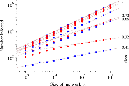
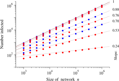
Figure 2: Simulation results for the number of vertices infected with each disease as a function of network size for various values of the parameters. Red circles indicate values for the red disease, blue squares for the blue disease. Each point represents an average over 1000 networks. In the top panel $\alpha=0.3$, $T_{b}=1$, and $T_{r}$ is 0.37, 0.42, 0.50, 0.55, and 0.75 for the various data sets shown. These parameter values are all outside the coexistence region, in the regime where one disease or the other always dominates. In the lower panel $\alpha=0.7$, $T_{b}=1$, and $T_{r}$ is 0.4, 0.5, 0.6, 0.8 and 1. These parameters include parts of the coexistence region, where both diseases can infect an extensive number of vertices. The dotted lines represent the scaling expected from the arguments given in the text.

Figure 2 shows the scaling of the numbers of infected individuals with network size for two different values of the parameter $\alpha$ (top and bottom panels in the figure). The red and blue points indicate the numerical results for the red and blue diseases, averaged over a thousand networks each, while the solid lines represent the expected slope of the scaling in the large-$n$ limit. As we can see, in most cases the numerical results appear to converge to the expected slope as $n$ becomes large, confirming our analytic calculations. For parameter values that fall close to the growth-rate boundary, however, the agreement is poorer (lines of slope 0.70 and 0.66 in the upper panel and 0.76 in the lower panel). We interpret this as an effect of the early-time fluctuations discussed in Section II. When we are close to the boundary, fluctuations in the early growth of one or both diseases can give the slower-growing disease a lead over the faster one large enough that the faster one never catches up. As a result the slower disease achieves $\mathrm{O}(n)$ scaling where normally it would have the lesser $\mathrm{O}(n^{\beta})$ [or $\mathrm{O}(n^{1/\beta})$]. When averaged over many simulations, this means that the apparent scaling of the number of infected individuals will lie somewhere between the expected $\mathrm{O}(n^{\beta})$ and the steeper $\mathrm{O}(n)$, which is what we see in Fig. 2.

In this regime, therefore, the observed behavior is a result of initial fluctuations coupled with finite-size effects. It should be possible to reduce the magnitude of the effect either by increasing the system size (so as to reduce finite-size effects) or by increasing the number of initial carriers of the disease (to reduce fluctuations). As we argued in Section II, however, one may have to increase the system size enormously—far beyond our ability to perform the simulations—in order to make a significant difference. And reducing early fluctuations by increasing the number of initial carriers has the undesirable result of increasing the finite-size effects, since it reduces the length of the exponential growth phase for both diseases, and therefore again requires us to increase the system size to get comparable results. In practice, therefore, there is no easy way to reach the asymptotic scaling regime when we are close to the growth-rate boundary.

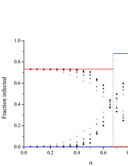
Figure 3: Simulation results for the average fraction of vertices infected with red (circles) and blue (squares) diseases as a function of $\alpha$ for the case $T_{r}=0.6$, $T_{b}=0.8$. Solid lines represent the analytic predictions for the same parameter values. The parameters fall outside the coexistence region for all values of $\alpha$, so one disease or the other should always dominate, at least in the limit of large $n$, and there should be a single discontinuous transition as we cross the growth-rate boundary. The shades of the data points indicate network sizes of $n=10^{3}$, $10^{4}$, $10^{5}$, and $10^{6}$ (lightest points to darkest). Each point is an average over at least $100$ networks.

In Fig. 3 we show results for the final fraction of individuals infected with each disease as a function of $\alpha$ for fixed $T_{b}$ and $T_{r}$. The value of $T_{r}$ is chosen to fall above the coexistence threshold $\phi_{x}$, so that we are in the regime on the right of the phase diagram, Fig. 1, where one disease, either red or blue, always wins and the other reaches a negligible fraction of vertices. The points on the plot represent the numerical results, while the red and blue lines show our analytic predictions from Eqs. (11) and (12). The lines are horizontal because the sizes of the epidemics depend only on the transmissibilities (which are fixed) and not on $\alpha$, except at the growth-rate boundary, which is clearly visible as the step where the dominant disease switches from red to blue.

As we can see from the figure the agreement between analytic and numerical results is good away from the growth-rate boundary, as we expect. Away from the boundary finite-size effects are small and fluctuations should have a negligible impact on outcomes. Closer to the boundary agreement is poorer because, once again, the plotted points represent averages over many simulations and in some of those simulations the “wrong” disease dominates because of chance fluctuations (or merely fails to be vanishingly small), moving the average away from the infinite-$n$ prediction. Moreover, in this regime convergence to the analytic prediction with increasing $n$ appears slow (represented by the varying shades of gray among the points), which accords qualitatively with our expectations from Eq. (2) and the accompanying argument.

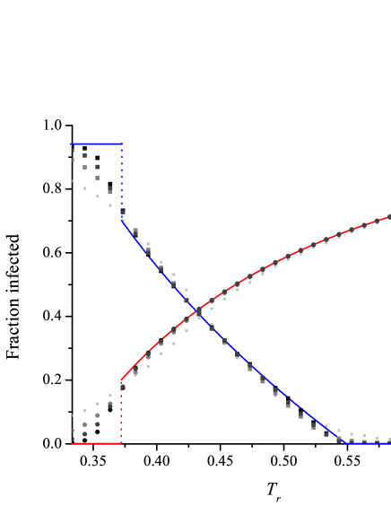
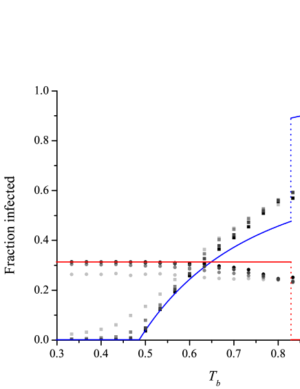
Figure 4: Top: simulation results for the average fraction of vertices infected with red (circles) and blue (squares) as a function of $T_{r}$ for the case $\alpha=0.1$, $T_{b}=1$. Bottom: the corresponding plot as a function of $T_{b}$ for $T_{r}=0.4$, $\alpha=0.2$. The solid lines represent the analytic predictions. The parameter ranges in each case were chosen to overlap the coexistence region so that two transitions are visible in each panel, the discontinuous transition at the growth-rate boundary and the continuous transition at the coexistence threshold. In the central region of each panel the two diseases coexist. As in Fig. 3, the shades of the data points indicate network sizes of $n=10^{3}$, $10^{4}$, $10^{5}$, and $10^{6}$ (lightest points to darkest). Each point is an average over at least $100$ networks.

In Fig. 4 we show two further plots of epidemic size, this time with $\alpha$ fixed and either $T_{r}$ (upper panel) or $T_{b}$ (lower panel) varying. Both plots include parameter ranges that fall within the coexistence regime and in each we can see both the discontinuous growth-rate transition and the continuous coexistence transition. As expected we see some finite-size rounding of the coexistence transition, particularly for smaller system sizes, and considerably more dramatic deviations from the analytic predictions around the growth-rate boundary, as in Fig. 3.

VI Epidemic sizes close to the growth-rate boundary

The numerical results of Section V agree well with our analytic predictions, except in the region close to the growth-rate boundary, where, as we have seen, the combination of finite-size effects and fluctuations in the early stages of the growth process can produce significant deviations from the expected behavior. In this regime the large-$n$ theory breaks down. We can, however, still derive some useful analytic results. As we show in this section, even though it is not possible to predict the final size of either of the two epidemics close to the growth-rate boundary, the sizes are still related to one another, one being large whenever the other is small, and we can derive constraints on the particular combinations of sizes allowed.

Again our calculations are for the configuration model. We consider a vertex anywhere in the network and one of the edges connected to that vertex, and we define $w$ to be the average probability that neither of the two diseases was transmitted to the vertex down that edge. By transmission we here mean that the pathogen was spread, but not that the vertex necessarily became infected—a vertex that was previously infected with either disease will not become infected again even if the pathogen is spread to it.

The probability that the red disease was spread over the edge in question is equal to the probability, denoted $q_{r}$, that the vertex at the other end was infected with red, times the probability that transmission occurred, which is $T_{r}$ by definition, for a total probability of $T_{r}q_{r}$. Similarly the probability for blue is $T_{b}q_{b}$, and the total probability $1-w$ that either disease is transmitted is $T_{r}q_{r}+T_{b}q_{b}$, so

$$w=1-T_{r}q_{r}-T_{b}q_{b}.$$ (27)

Now suppose that the vertex at the end of the edge has excess degree $k$. Then the probability that it is infected with neither red nor blue is equal to the probability that neither disease was transmitted to it along any of its $k$ edges, which is $w^{k}$. Averaging over the excess degree distribution $q_{k}$, the vertex’s average probability of being uninfected is thus $\sum_{k}q_{k}w^{k}=F_{1}(w)$, where $F_{1}$ is the generating function for the excess degree distribution, as previously. Then the probability that the vertex is infected is $1-F_{1}(w)$, which is necessarily equal to $q_{r}+q_{b}$. Thus we have

$$F_{1}(w)=1-q_{r}-q_{b}.$$ (28)

Substituting for $w$ from Eq. (27), we then have

$$F_{1}(1-T_{r}q_{r}-T_{b}q_{b})=1-q_{r}-q_{b}.$$ (29)

This equation does not uniquely determine either of the probabilities $q_{r}$ or $q_{b}$, and indeed, as we have seen, for finite-size networks they are typically not determined but can take a range of values depending on chance fluctuations. But Eq. (29) gives us a relation between the two such that if we know either one then we know the other.

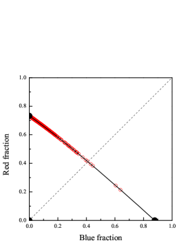
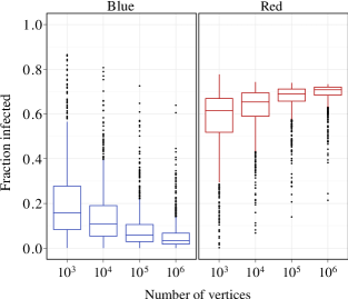
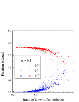
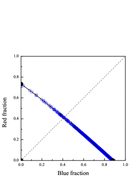
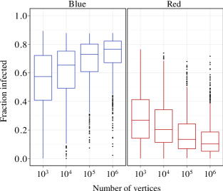
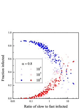
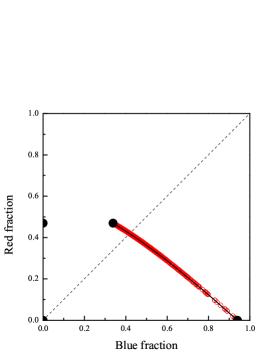
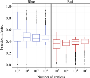
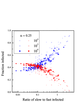
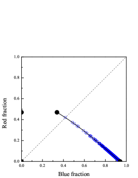
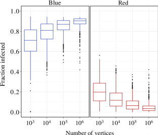
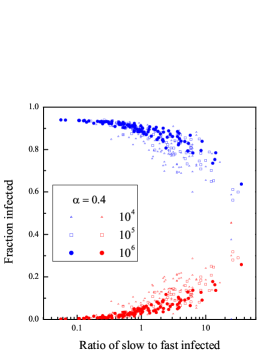
Figure 5: Simulation results comparing the fractions of vertices infected with the red and blue diseases for four different sets of parameter values close to the growth-rate boundary (the four rows in the figure). Left column: the fraction infected with red versus blue for networks with $n=10^{6}$. All points lie on the curves defined by Eq. (29), which are shown as the solid black lines. Middle column: box plot of the fraction infected with each disease for various network sizes $n$. Right column: the fraction infected with each disease at the end of the simulation as a function of the ratio of the numbers infected by the faster- and slower-growing diseases measured at the first time that either disease reaches $\mbox{$\frac{1}{2}$}\sqrt{n}$. First row: $T_{b}=0.8$, $T_{r}=0.6$, $\alpha=0.5$; second row: $T_{b}=0.8$, $T_{r}=0.6$, $\alpha=0.8$; third row: $T_{b}=1$, $T_{r}=0.45$, $\alpha=0.25$; fourth row: $T_{b}=1$, $T_{r}=0.45$, $\alpha=0.4$.

In Fig. 5 we test Eq. (29) against the results of numerical simulations. We again take a Poisson degree distribution, for which, conveniently, since the degree and excess degree distributions are identical, the probabilities $q_{r}$ and $q_{b}$ that the vertex at the end of an edge is infected with red or blue are equal to the overall fractions $p_{r}$ and $p_{b}$ of red and blue vertices in the network as a whole. For four different sets of values of the model parameters close to the growth-rate boundary (the four rows in Fig. 5) we measure these two fractions on 1000 different networks and in the left column of Fig. 5 we show scatter plots of $p_{r}$ against $p_{b}$. The solid lines in the plots represent Eq. (29) and, as we can see, the values of $p_{r}$ and $p_{b}$ indeed lie along this line. On any particular run of the simulation one cannot predict where the individual values $p_{r}$ and $p_{b}$ will fall, but if we know one then we can predict the other, since they always fall on this line. (The lines appear straight in the figure, but are in fact slightly curved for this particular choice of degree distribution and model parameters.)

Of the four rows in the figure, the first two have the same values of $T_{r}$ and $T_{b}$, chosen to fall above the coexistence threshold in the regime where coexistence does not occur, and two different values of $\alpha$ chosen to fall a little below and a little above the growth-rate boundary. Thus for the parameter values in the first row the red disease is faster growing and would dominate in the limit of large $n$ but the blue one occasionally wins on the finite network. The second column gives a box plot showing the average fraction infected with each disease for a range of system sizes $n$, and we can see that as $n$ becomes larger the dominance of red becomes progressively better defined. In the second row of the figure blue is the faster growing disease and the positions are reversed, blue winning more often, particularly as $n$ becomes large.

The third and fourth rows of Fig. 5 show similar results, but for $T_{r}$ below the coexistence threshold. Now when $\alpha$ is chosen to put us below the growth-rate boundary, in the coexistence region (third row in the figure), we see that neither red nor blue dominates, even for large $n$, with both infecting significant fractions of the network. In the fourth and final row of the figure the value of $\alpha$ places us above the growth-rate boundary again and in this regime blue dominates in the limit of large $n$.

These results accord well with the analysis presented earlier. We have not, however, directly tested our hypothesis that the deviations we observe from the infinite-$n$ results are due to stochastic fluctuations in the early stages of the growth process. The third column of Fig. 5 shows a test of this hypothesis. The test involves waiting an initial period of time for the fluctuations to become small, then measuring the number of individuals infected with each disease. The horizontal axis in each panel of the third column gives the ratio of the number of vertices infected by the disease (either red or blue) with the slower exponential growth rate versus the number infected by the disease with the faster, measured at the first moment that either disease reaches $\mbox{$\frac{1}{2}$}\sqrt{n}$ infected individuals. The vertical axis measures the final fraction of individuals infected with each disease, once both have run their course, and the scatter of red and blue points shows the results for each of our simulations, for a range of different network sizes.

On the left-hand side of each graph in the third column the ratio of slow- to fast-growing diseases is small, meaning that the fast-growing one dominates at early times. In these circumstances, if we assume that fluctuations are no longer important to the fast-growing disease and that it simply grows exponentially with the appropriate growth rate, then the final size of its outbreak is uniquely determined, and hence so is the final size of the outbreak of the slower disease. The results in the figure appear to confirm this conjecture, with the observed fractions infected with each disease being narrowly concentrated around single values. As we move further to the right, we enter the regime in which the slower growing disease infects more individuals at early times. In this regime, and particularly in the rightmost regions of the graph, the faster growing disease only infects a small number of individuals and hence can have significant fluctuations. These fluctuations may give the fast-growing disease a boost sufficient to allow it to catch up to the slower one, or a delay sufficient to ensure that it does not. Thus in this region the outcome is not uniquely determined and we expect to see a range of final infected fractions. Again the numerical results shown in the figure appear to confirm this conjecture, with a much broader scatter of points on the right than on the left. Finally, note that the points in the right-hand part of the figure are primarily those for simulations on smaller networks (as indicated by the shapes of the points), because larger systems take longer to reach the $\mbox{$\frac{1}{2}$}\sqrt{n}$ point, making the typical values of the slow-to-fast ratio (which dwindles over time) smaller and hence pushing the points leftward on the plot as $n$ grows.

VII Conclusion

In this paper we have studied the behavior of two competing diseases with complete cross-immunity (or two strains of a single disease) spreading concurrently over a static network of contacts between individuals of a single population. Using a mixture of analytic results, heuristic arguments, and numerical simulation, we have derived the phase diagram for the system, which shows four distinct phases, and given calculations of the expected number of individuals infected with each of the diseases in the limit of large network size for networks generated using the configuration model. Of particular interest is the coexistence phase, a region of the parameter space in which neither disease excludes the other and both spread to infect an extensive fraction of the network. We have demonstrated a number of nontrivial features of this phase, including the fact that the disease that expands through the population slower must nonetheless have a higher probability of transmission if coexistence is to occur. Such behavior is possible only if the faster growing disease has a shorter transmission time between when an individual gets infected and when they pass on the infection to others, and we have shown also that there is an upper bound on the ratio of the transmission times of the two diseases if coexistence is to occur.

Another unusual feature of the system is the “growth-rate boundary,” a dynamical transition between regimes in which one disease or the other dominates. The numbers of individuals infected by both diseases change discontinuously as we cross this boundary, in the limit of large system size, although for finite systems the transition is blurred by strong finite-size effects.

A number of extensions or generalizations of our calculations are possible. We have worked with the simplest possible model of epidemic dynamics, the Reed–Frost model, but calculations could be performed for other SIR-style models, such as the Kermack–McKendrick model in which infection and recovery processes take place in continuous time with stochastically constant rates. The results should be qualitatively similar: one expects to see a growth-rate boundary in any model with exponential growth rates. Extending the model further, one could introduce arbitrary distributions of transmission and recovery times KN10a , but determining the exponential growth rates will be more complicated for such a system. Changes of this kind may alter the shape of the growth-rate boundary but should not change the qualitative nature of the transition.

There are also some questions of interest concerning the Reed–Frost model that are not answered by the calculations presented here. Our analytic results are all derived for the configuration model and different behaviors might be seen on other networks. Also, close to the growth-rate boundary we observe strong finite-size deviations from the large-$n$ predictions of the analytic theory, and it is unclear at present how to calculate, for instance, the exponents characterizing the growth of epidemics with system size in this regime. And we have assumed in our calculations that neither disease dies out in the early stages of the growth process; in reality they will sometimes die out and we do not at present know how to calculate the probabilities of certain outcomes, such as the probability within the coexistence region that the slower-growing disease will die out after the faster-growing one has spread. This probability depends on the chance that the slower disease reaches the giant component of the residual network, a probability that does not appear to have a simple expression in the percolation-theory language employed here. These and other interesting questions we leave for future work.

- (1) R. M. Anderson and R. M. May, Infectious Diseases of Humans. Oxford University Press, Oxford (1991).
- (2) H. W. Hethcote, The mathematics of infectious diseases. SIAM Review 42, 599–653 (2000).
- (3) M. J. Keeling and K. T. James, Networks and epidemic models. J. R. Soc. Interface 2, 295–307 (2005).
- (4) F. Liljeros, C. R. Edling, L. A. N. Amaral, H. E. Stanley, and Y. Åberg, The web of human sexual contacts. Nature 411, 907–908 (2001).
- (5) R. Pastor-Satorras and A. Vespignani, Epidemic spreading in scale-free networks. Phys. Rev. Lett. 86, 3200–3203 (2001).
- (6) M. E. J. Newman, Spread of epidemic disease on networks. Phys. Rev. E 66, 016128 (2002).
- (7) S. Bansal, B. T. Grenfell, and L. A. Meyers, When individual behavior matters: homogeneous and network models in epidemiology. J. R. Soc. Interface 4, 879–891 (2007).
- (8) E. Kenah and J. C. Miller, Epidemic percolation networks, epidemic outcomes, and interventions. Interdisciplinary Perspectives on Infectious Diseases 2011, 543520 (2011).
- (9) P. S. Dodds and D. J. Watts, Universal behavior in a generalized model of contagion. Phys. Rev. Lett. 92, 218701 (2004).
- (10) D. Mollison, Spatial contact models for ecological and epidemic spread. Journal of the Royal Statistical Society B 39, 283–326 (1977).
- (11) P. Grassberger, On the critical behavior of the general epidemic process and dynamical percolation. Math. Biosci. 63, 157–172 (1983).
- (12) L. M. Sander, C. P. Warren, I. Sokolov, C. Simon, and J. Koopman, Percolation on disordered networks as a model for epidemics. Math. Biosci. 180, 293–305 (2002).
- (13) M. E. J. Newman, Threshold effects for two pathogens spreading on a network. Phys. Rev. Lett. 95, 108701 (2005).
- (14) S. Funk and V. A. A. Jansen, Interacting epidemics on overlay networks. Phys. Rev. E 81, 036118 (2010).
- (15) Y.-Y. Ahn, H. Jeong, N. Masuda, and J. D. Noh, Epidemic dynamics of two species of interacting particles on scale-free networks. Phys. Rev. E 74, 066113 (2006).
- (16) M. Molloy and B. Reed, A critical point for random graphs with a given degree sequence. Random Structures and Algorithms 6, 161–179 (1995).
- (17) M. E. J. Newman, S. H. Strogatz, and D. J. Watts, Random graphs with arbitrary degree distributions and their applications. Phys. Rev. E 64, 026118 (2001).
- (18) For technical reasons we also require that the first and second moments of the degree distribution be finite.
- (19) R. Cohen, K. Erez, D. ben-Avraham, and S. Havlin, Resilience of the Internet to random breakdowns. Phys. Rev. Lett. 85, 4626–4628 (2000).
- (20) D. S. Callaway, M. E. J. Newman, S. H. Strogatz, and D. J. Watts, Network robustness and fragility: Percolation on random graphs. Phys. Rev. Lett. 85, 5468–5471 (2000).
- (21) The definition of the coexistence threshold used here differs slightly from that used in Ref. Newman05c . In that paper the threshold was defined as the transmissibility above which coexistence is impossible for any value of , no matter how large, whereas it is defined here to be the transmissibility for the actual value of . Equivalently, the definition used in Newman05c is equal to our definition when takes its maximum value of 1.
- (22) V. Marceau, P.-A. Noël, L. Hébert-Dufresne, A. Allard, and L. J. Dubé, Modeling the dynamical interaction between epidemics on overlay networks. Preprint arxiv:1103.4059 (2011).
- (23) Strictly speaking, at , Eqs. (6) and (8) should read and because the initial carriers of the diseases are chosen at random and not infected via a neighbor. In real life, on the other hand, all infections are acquired via a neighbor, so the equations should always be correct. These subtleties do not affect our arguments, however, so we ignore them here.
- (24) A naive implementation of this scheme would be computationally wasteful, and also somewhat arbitrary since one would have to decide a threshold level of infection below which a disease would be deemed to have died out. In our simulations we mitigate these problems somewhat by first generating the bond percolation clusters for the entire network and starting the simulated spread of the two diseases at vertices chosen from the giant clusters. This does not guarantee that both diseases will produce an epidemic in the coexistence region but it reduces substantially the number of cases where a disease dies out.
- (25) B. Karrer and M. E. J. Newman, A message passing approach for general epidemic models. Phys. Rev. E 82, 016101 (2010).