Asymptotic Inference of Autocovariances of Stationary Processes

Abstract

The paper presents a systematic theory for asymptotic inference of autocovariances of stationary processes. We consider nonparametric tests for serial correlations based on the maximum (or ${\cal L}^{\infty}$) and the quadratic (or ${\cal L}^{2}$) deviations. For these two cases, with proper centering and rescaling, the asymptotic distributions of the deviations are Gumbel and Gaussian, respectively. To establish such an asymptotic theory, as byproducts, we develop a normal comparison principle and propose a sufficient condition for summability of joint cumulants of stationary processes. We adopt a simulation-based block of blocks bootstrapping procedure that improves the finite-sample performance.

thebibliographysize

and

1 Introduction

If $(X_{i})_{i\in\mathbb{Z}}$ is a real-valued stationary process, then from a second-order inference point of view it is characterized by its mean $\mu=\mathbb{E}X_{i}$ and the autocovariance function $\gamma_{k}=\mathbb{E}[(X_{0}-\mu)(X_{k}-\mu)]$, $k\in\mathbb{Z}$. Assume $\mu=0$. Given observations $X_{1},\ldots,X_{n}$, the natural estimates of $\gamma_{k}$ and the autocorrelation $r_{k}=\gamma_{k}/\gamma_{0}$ are

$$\hat{\gamma}_{k}=(1/n)\sum_{i=|k|+1}^{n}X_{i-|k|}X_{i}\quad\hbox{and}\quad\hat{r}_{k}=\hat{\gamma}_{k}/\hat{\gamma}_{0},\,\,1-n\leq k\leq n-1,$$ (1)

respectively. The estimator $\hat{\gamma}_{k}$ plays a crucial role in almost every aspect of time series analysis. It is well-known that for linear processes with independent and identically distributed (iid) innovations, under suitable conditions, $\sqrt{n}(\hat{\gamma}_{k}-\gamma_{k})\Rightarrow\mathcal{N}(0,\tau_{k}^{2})$, where $\Rightarrow$ stands for convergence in distribution, $\mathcal{N}(0,\tau_{k}^{2})$ denotes the normal distribution with mean zero and variance $\tau_{k}^{2}$. Here $\tau_{k}^{2}$ can be calculated by Bartlett’s formula (see Section 7.2 of Brockwell and Davis (1991)). Other contributions on linear processes include Hannan and Heyde (1972), Hosoya and Taniguchi (1982), Anderson (1991) and Phillips and Solo (1992) etc. Romano and Thombs (1996) and Wu (2009) considered the asymptotic normality of $\hat{\gamma}_{k}$ for nonlinear processes. As a primary goal of the paper, we shall study asymptotic properties of the quadratic (or ${\cal L}^{2}$) and the maximum (or ${\cal L}^{\infty}$) deviations of $\hat{\gamma}_{k}$.

1.1 The ${\cal L}^{2}$ Theory

Testing for serial correlation has been extensively studied in both statistics and econometrics, and it is a standard diagnostic procedure after a model is fitted to a time series. Classical procedures include Durbin and Watson (1950, 1951), Box and Pierce (1970), Robinson (1991) and their variants. The Box-Pierce portmanteau test uses $Q_{K}=n\sum_{k=1}^{K}\hat{r}_{k}^{2}$ as the test statistic, and rejects if it lies in the upper tail of $\chi^{2}_{K}$ distribution. An arguable deficiency of this test and many of its modified versions (for a review see for example Escanciano and Lobato (2009)) is that the number of lags $K$ included in the test is held as a constant in the asymptotic theory. As commented by Robinson (1991):

”…unless the statistics take account of sample autocorrelations at long lags there is always the possibility that relevant information is being neglected…”

The problem is particularly relevant if practitioners have no prior information about the alternatives. The attempt of incorporating more lags emerged naturally in the spectral domain analysis; see among others Durlauf (1991), Hong (1996) and Deo (2000). The normalized spectral density $f(\omega)=(2\pi)^{-1}\sum_{k\in\mathbb{Z}}r_{k}\cos(k\omega)$ should equal to $(2\pi)^{-1}$ when the serial correlation is not present. Let $\hat{f}(\omega)=\sum_{k=1-n}^{n-1}h(k/s_{n})\hat{r}_{k}\cos(k\omega)$ be the lag-window estimate of the normalized spectral density, where $h(\cdot)$ is a kernel function and $s_{n}$ is the bandwidth satisfying the natural condition $s_{n}\to\infty$ and $s_{n}/n\to 0$. The former aims to include correlations at large lags. A test for the serial correlation can be obtained by comparing $\hat{f}$ and the constant function $f(\omega)\equiv(2\pi)^{-1}$ using a suitable metric. In particular, using the quadratic metric and rectangle kernel, the resulting test statistic is the Box-Pierce statistic with unbounded lags. Hong (1996) established the following result:

$$\frac{1}{\sqrt{2s_{n}}}\left(n\sum_{k=1}^{s_{n}}(\hat{r}_{k}-r_{k})^{2}-s_{n}\right)\Rightarrow\mathcal{N}(0,1),$$ (2)

under the condition that $X_{i}$ are iid, which implies that all $r_{k}$ in the preceding equation are zero. Lee and Hong (2001) and Duchesne, Li and Vandermeerschen (2010) studied similar tests in spectral domain, but using a wavelet basis instead of trigonometric polynomials in estimating the spectral density and henceforth working on wavelet coefficients. Fan (1996) considered a similar problem in a different context and proposed adapative Neyman test and thresholding tests, using $\max_{1\leq k\leq s_{n}}(Q_{k}-k)/\sqrt{2k}$ and $n\sum_{k=1}^{s_{n}}\hat{r}_{k}^{2}I(|\hat{r}_{k}|>\delta)$ as test statistics respectively, where $\delta$ is a threshold value. Escanciano and Lobato (2009) proposed to use $Q_{s_{n}}$ with $s_{n}$ being selected by AIC or BIC.

It has been an important and difficult question on whether the iid assumption in Hong (1996) can be relaxed. Similar problems have been studied by Durlauf (1991), Deo (2000) and Hong and Lee (2003) for the case that $X_{i}$ are martingale differences. Recently Shao (2011) showed that (2) is true when $(X_{i})$ is a general white noise sequence, under the geometric moment contraction (GMC) condition. Since the GMC condition, which implies that the autocovariances decay geometrically, is quite strong, the question arises as to whether it can be replaced by a weaker one. Furthermore, one may naturally ask: what if the serial correlation is present in (2)? To the best of our knowledge, there has been no results in the literature for this problem. This paper shall address these questions and substantially generalizes earlier results. We shall prove that (2) remains true even if all or some of $r_{k}$ are not zero, but the variance of the limiting distribution, being different, will depend on the values of $r_{k}$. Furthermore, we derive the limiting distribution of $\sum_{k=1}^{s_{n}}\hat{r}_{k}^{2}$ when the serial correlation is present. The latter result enables us to calculate the asymptotic power of the Box-Pierce test with unbounded lags.

1.2 The ${\cal L}^{\infty}$ Theory

Another natural omnibus choice is to use the maximum autocorrelation as the test statistic. Wu (2009) obtained a stochastic upper bound for

$$\sqrt{n}\max_{1\leq k\leq s_{n}}|\hat{\gamma}_{k}-\gamma_{k}|,$$ (3)

and argued that in certain situations the test based on (3) has a higher power over the Box-Pierce tests with unbounded lags in detecting weak serial correlation. It turns out that the uniform convergence of autocovariances is also closely related to the estimation of orders of ARMA processes or linear systems in general. The pioneer works in this direction were given by E. J. Hannan and his collaborators, see for example Hannan (1974) and An, Chen and Hannan (1982). For a summary of these works we recommend (Hannan and Deistler, 1988, Section §5.3) and references therein. In particular, An, Chen and Hannan (1982) showed that if $s_{n}=O[(\log n)^{\alpha}]$ for some $\alpha<\infty$, then with probability one

$$\sqrt{n}\max_{1\leq k\leq s_{n}}|\hat{\gamma}_{k}-\gamma_{k}|=O\left(\log\log n\right).$$ (4)

The question of deriving the asymptotic distribution of (3) is more challenging. Although Wu (2009) was not able to obtain the limiting distribution of (3), his work provided important insights into this problem. Assuming $k_{n}\to\infty$, $k_{n}/n\to 0$ and $h\geq 0$, he showed that, for $T_{k}=\sqrt{n}(\hat{\gamma}_{k}-\mathbb{E}\hat{\gamma}_{k})$,

$$\left(T_{k_{n}}\,,\,T_{k_{n}+h}\right)^{\top}\Rightarrow\mathcal{N}\left[0,\begin{pmatrix}\sigma_{0}&\sigma_{h}\\ \sigma_{h}&\sigma_{0}\end{pmatrix}\right],\quad\hbox{where }\sigma_{h}=\sum_{k\in\mathbb{Z}}\gamma_{k}\gamma_{k+h},$$ (5)

and we use the superscript $\top$ to denote the transpose of a vector or a matrix. The asymptotic distribution in (5) does not depend on the speed of $k_{n}\to\infty$. It suggests that, at large lags, the covariance structure of $(T_{k})$ is asymptotically equivalent to that of the Gaussian sequence

$$(G_{k}):=\left(\sum_{i\in\mathbb{Z}}\gamma_{i}\eta_{i-k}\right)$$ (6)

where $\eta_{i}$’s are iid standard normal random variables. Define the sequences $(a_{n})$ and $(b_{n})$ as

$$a_{n}=(2\log n)^{-1/2}\,\,\hbox{ and }\,\,b_{n}=(2\log n)^{1/2}-(8\log n)^{-1/2}(\log\log n+\log 4\pi).$$ (7)

According to Berman (1964) (also see Remarks 3 and 4), under the condition $\lim_{n\to\infty}\mathbb{E}(G_{0}G_{n})\log n=0$,

$$\lim_{s\to\infty}P\left(\max_{1\leq i\leq s}|G_{i}|\leq\sqrt{\sigma_{0}}(a_{2s}\,x+b_{2s})\right)=\exp\{-\exp(-x)\}.$$

Therefore, Wu (2009) conjectured that under suitable conditions, one has the Gumbel convergence

$$\lim_{n\to\infty}P\left(\max_{1\leq k\leq s_{n}}|T_{k}|\leq\sqrt{\sigma_{0}}(a_{2s_{n}}\,x+b_{2s_{n}})\right)=\exp\{-\exp(-x)\}.$$ (8)

In a recent work, Jirak (2011) proved this conjecture for linear processes and for $s_{n}$ growing with at most logarithmic speed. We shall prove (8) in Section 4 for general stationary processes; and our result allows $s_{n}$ to grow as $s_{n}=O(n^{\eta})$ for some $0<\eta<1$, and $\eta$ can be arbitrarily close to $1$ under appropriate moment and dependence conditions. The latter result substantially relaxes the severe restriction on the growth speed in (4) and Jirak (2011) and, moreover, the obtained distributional convergence are more useful for statistical inference. For example, other than testing for serial correlation and estimating the order of a linear system, (8) can also be used to construct simultaneous confidence intervals of autocovariances.

1.3 Relations with the Random Matrix Theory

In a companion paper, using the asymptotic theory of sample autocovariances developed in this paper, Xiao and Wu (2010) studied convergence properties of estimated covariance matrices which are obtained by banding or thresholding. Their bounds are analogs under the time series context to those of Bickel and Levina (2008b, a). There is an important difference between these two settings: we assume that only one realization is available, while Bickel and Levina (2008b, a) require multiple iid copies of the underlying random vector.

There has been some related works in the random matrix theory literature that are similar to (8). Suppose one has $n$ iid copies of a $p$-dimensional random vector, forming a $p\times n$ data matrix $\boldsymbol{X}$. Let $\hat{r}_{ij}$, $1\leq i,j\leq p$, be the sample correlations. Jiang (2004) showed that the limiting distribution of $\max_{1\leq i<j\leq p}|\hat{r}_{ij}|$, after suitable normalization, is Gumbel provided that each column of $\boldsymbol{X}$ consists of $p$ iid entries and each entry has finite moment of some order higher than 30, and $p/n$ converges to some constant. His work was followed and improved by Zhou (2007) and Liu, Lin and Shao (2008). In a recent article, Cai and Jiang (2010) extended those results in two ways: (i) the dimension $p$ could grow exponentially as the sample size $n$ provided exponential moment conditions; and (ii) they showed that the test statistic $\max_{|i-j|>s_{n}}|\hat{r}_{ij}|$ also converges to the Gumbel distribution if each column of $\boldsymbol{X}$ is Gaussian and is $s_{n}$-dependent. The latter generalization is important since it is one of the very few results that allow dependent entries. Their method is Poisson approximation (see for example Arratia, Goldstein and Gordon, 1989), which heavily depends on the fact that for each sample correlation to be considered, the corresponding entries are independent. Schott (2005) proved that $\sum_{1\leq i<j\leq p}\hat{r}_{ij}^{2}$ converges to normal distribution after suitable normalization, under the conditions that each column of $\boldsymbol{X}$ contains iid Gaussian entries and $p/n$ converges to some positive constant. His proof heavily depends on the normality assumption. Techniques developed in those papers are not applicable here since we have only one realization and the dependence structure among the entries can be quite complicated.

1.4 A Summary of Results of the Paper

We present the main results in Section 2, which include a central limit theory of (2) and the Gumbel convergence (8). The proofs are given in Section 4. In Section 5 we prove a normal comparison principle, which is of independent interest. Since summability conditions of joint cumulants are commonly used in time series analysis (see for example Brillinger (2001) and Rosenblatt (1985)) and is needed in the proof of Theorem 4, we present a sufficient condition in Section 6. Some auxiliary lemmas are collected in Section 7. We also conduct a simulation study in Section 3, where we design a simulation-based block of blocks bootstrapping procedure that improves the finite-sample performance.

2 Main Results

To develop an asymptotic theory for time series, it is necessary to impose suitable measures of dependence and structural assumptions for the underlying process $(X_{i})$. Here we shall adopt the framework of Wu (2005). Assume that $(X_{i})$ is a stationary causal process of the form

$$X_{i}=g(\cdots,\epsilon_{i-1},\epsilon_{i}),$$ (9)

where $\epsilon_{i},i\in\mathbb{Z}$, are iid random variables, and $g$ is a measurable function for which $X_{i}$ is a properly defined random variable. For notational simplicity we define the operator $\Omega_{k}$: suppose $X=h(\epsilon_{j},\epsilon_{i-1},\ldots)$ is a random variable which is a function of the innovations $\epsilon_{l},l\leq j$, then $\Omega_{k}(X):=h(\epsilon_{j},\ldots,\epsilon_{k+1},\epsilon_{k}^{\prime},\epsilon_{k-1},\ldots)$, where $(\epsilon_{k}^{\prime})_{k\in\mathbb{Z}}$ is an iid copy of $(\epsilon_{k})_{k\in\mathbb{Z}}$. Namely $\epsilon_{k}$ in $X$ is replaced by $\epsilon_{k}^{\prime}$.

For a random variable $X$ and $p>0$, we write $X\in\mathcal{L}^{p}$ if $\|X\|_{p}:=(\mathbb{E}|X|^{p})^{1/p}<\infty$, and in particular, use $\|X\|$ for the $\mathcal{L}^{2}$-norm $\|X\|_{2}$. Assume $X_{i}\in\mathcal{L}^{p}$, $p>1$. Define the physical dependence measure of order $p$ as

$$\delta_{p}(i)=\|X_{i}-\Omega_{0}(X_{i})\|_{p},$$ (10)

which quantifies the dependence of $X_{i}$ on the innovation $\epsilon_{0}$. Our main results depend on the decay rate of $\delta_{p}(i)$ as $i\to\infty$. Let $p^{\prime}=\min(2,p)$ and define

$$\Theta_{p}(n) = \sum_{i=n}^{\infty}\delta_{p}(i),\quad\Psi_{p}(n)=\left(\sum_{i=n}^{\infty}\delta_{p}(i)^{p^{\prime}}\right)^{1/p^{\prime}},\quad\hbox{and}\quad$$ (11)

$$\Delta_{p}(n) = \sum_{i=0}^{\infty}\min\{\mathcal{C}_{p}\Psi_{p}(n),\delta_{p}(i)\},$$ (12)

where $\mathcal{C}_{p}$ is defined in (31). It is easily seen that $\Psi_{p}(\cdot)\leq\Theta_{p}(\cdot)\leq\Delta_{p}(\cdot)$. We use $\Theta_{p}$, $\Psi_{p}$ and $\Delta_{p}$ as shorthands for $\Theta_{p}(0)$, $\Psi_{p}(0)$ and $\Delta_{p}(0)$ respectively. We make the convention that $\delta_{p}(k)=0$ for $k<0$.

There are several reasons that we use the framework (9) and the dependence measure (10). First, the class of processes that (9) represents is huge and it includes linear processes, bilinear processes, Volterra processes, and many other time series models. See, for instance, Tong (1990) and Wiener (1958). Second, the physical dependence measure is easy to work with and it is directly related to the underlying data-generating mechanism. Third, it enables us to develop an asymptotic theory for complicated statistics of time series.

2.1 Maximum deviations of sample autocovariances

Note that $\hat{\gamma}_{k}$ is a biased estimate of $\gamma_{k}$ with $\mathbb{E}\hat{\gamma}_{k}=(1-|k|/n)\gamma_{k}$. It is then more convenient to consider the centered version $\max_{1\leq k\leq s_{n}}\sqrt{n}|\hat{\gamma}_{k}-\mathbb{E}\hat{\gamma}_{k}|$ instead of $\max_{1\leq k\leq s_{n}}\sqrt{n}|\hat{\gamma}_{k}-\gamma_{k}|$. Recall (7) for $a_{n}$ and $b_{n}$.

Theorem 1.

Assume $\mathbb{E}X_{i}=0$, $X_{i}\in\mathcal{L}^{p}$ for some $p>4$, and $\Theta_{p}(m)=O(m^{-\alpha})$, $\Delta_{p}(m)=O(m^{-\alpha^{\prime}})$ for some $\alpha\geq\alpha^{\prime}>0$. If $s_{n}$ satisfies $s_{n}\to\infty$ and $s_{n}=O(n^{\eta})$ with

$$0<\eta<1,\quad\eta<\alpha p/2,\,\,\,\hbox{and}\,\,\,\eta\min\{2(p-2-\alpha p),\,(1-2\alpha^{\prime})p\}<p-4,$$ (13)

then for all $x\in\mathbb{R}$,

$$\lim_{n\to\infty}P\left(\max_{1\leq k\leq s_{n}}|\sqrt{n}[\hat{\gamma}_{k}-(1-k/n)\gamma_{k}]|\leq\sqrt{\sigma_{0}}(a_{2s_{n}}\,x+b_{2s_{n}})\right)=\exp\{-\exp(-x)\}.$$ (14)

In (13), if $p\leq 2+\alpha p$ or $1\leq 2\alpha^{\prime}$, then the second and third conditions are automatically satisfied, and hence Theorem 1 allows a very wide range of lags $s_{n}=O(n^{\eta})$ with $0<\eta<1$. In this sense Theorem 1 is nearly optimal.

For the maximum deviation $\max_{1\leq k<n}|\hat{\gamma}_{k}-\mathbb{E}\hat{\gamma}_{k}|$ over the whole range $1\leq k<n$, it seems not possible to derive a limiting distribution by using our method. However, we can obtain a sharp bound $(n^{-1}\log n)^{1/2}$. The upper bound is given in (16), while the lower bounded can be obtained by applying Theorem 1 and choosing a sufficiently small $\eta$ such that (13) holds. Using Theorem 2, Xiao and Wu (2010) derived convergence rates for the thresholded autocovariance matrix estimates.

Theorem 2.

Assume $\mathbb{E}X_{i}=0$, $X_{i}\in\mathcal{L}^{p}$ for some $p>4$, and $\Theta_{p}(m)=O(m^{-\alpha})$, $\Delta_{p}(m)=O(m^{-\alpha^{\prime}})$ for some $\alpha\geq\alpha^{\prime}>0$. If

$$\alpha>1/2\quad\hbox{or}\quad\alpha^{\prime}p>2$$ (15)

then for $c_{p}=6(p+4)\,e^{p/4}\,\kappa_{4}\,\Theta_{4}$,

$$\lim_{n\to\infty}P\left(\max_{1\leq k<n}|\hat{\gamma}_{k}-\mathbb{E}\hat{\gamma}_{k}|\leq c_{p}\sqrt{\frac{\log n}{n}}\right)=1.$$ (16)

Since $\Theta_{p}(m)\geq\Psi_{p}(m)$, we can assume $\alpha\geq\alpha^{\prime}$. For a detailed discussion on their relationship, see Remark 6 of Xiao and Wu (2010). It turns out that for the special case of linear processes the condition (13) can be weakened to the following one:

$$0<\eta<1,\quad\eta<\alpha p/2,\quad\hbox{and}\quad(1-2\alpha)\eta<(p-4)/p.$$ (17)

See Remark 2. Furthermore, for linear processes the condition (15) can be relaxed to $\alpha p>2$ as well.

In practice, the mean $\mu=\mathbb{E}X_{0}$ is often unknown and we can estimate it by the sample mean $\bar{X}_{n}=(1/n)\sum_{i=1}^{n}X_{i}$. The usual estimates of autocovariances and autocorrelations are

$$\breve{\gamma}_{k}=\frac{1}{n}\sum_{i=k+1}^{n}(X_{i-k}-\bar{X}_{n})(X_{i}-\bar{X}_{n})\quad\hbox{and}\quad\breve{r}_{k}=\breve{\gamma}_{k}/\breve{\gamma}_{0}.$$ (18)

Corollary 3.

Theorem 1 and Theorem 2 still hold if we replace $\hat{\gamma}_{k}$ therein by $\breve{\gamma}_{k}$. Furthermore,

$$\lim_{n\to\infty}P\left(\max_{1\leq k\leq s_{n}}\left|\sqrt{n}[\breve{r}_{k}-(1-k/n)r_{k}]\right|\leq(\sqrt{\sigma_{0}}/\gamma_{0})(a_{2s_{n}}\,x+b_{2s_{n}})\right)=\exp\{-\exp(-x)\}.$$

Proof of Corollary 3.

For the $\breve{\gamma}_{k}$ version of Theorem 1, it suffices to show that

$$\max_{1\leq k\leq s_{n}}\left|\sqrt{n}(\breve{\gamma}_{k}-\hat{\gamma}_{k})\right|=o_{P}\left(\frac{1}{\sqrt{\log s_{n}}}\right).$$ (19)

Let $S_{k}=\sum_{i=1}^{k}X_{i}$. By Theorem 1 (iii) of Wu (2007), we have $\left\|\max_{1\leq k\leq n}\left|S_{k}\right|\right\|\leq 2\sqrt{n}\Theta_{2}$. Since

$$\sum_{i=k+1}^{n}(X_{i-k}-\bar{X}_{n})(X_{i}-\bar{X}_{n})-\sum_{i=k+1}^{n}X_{i-k}X_{i} =-\bar{X}_{n}\sum_{i=1}^{n-k}X_{i}+\bar{X}_{n}\sum_{i=1}^{k}X_{i}-k\bar{X}_{n}^{2},$$

we have (19). The proof of the $\breve{\gamma}_{k}$ version of Theorem 2 is similar. The assertion on sample autocorrelations can be proved easily, and details are omitted. ∎

2.2 Box-Pierce tests

Box-Pierce tests (Box and Pierce, 1970; Ljung and Box, 1978) are commonly used in detecting lack of fit of a particular time series model. After a correct model has been fitted to a set of observations, one would expect the residuals to be close to a sequence of iid random variables, and therefore one should perform some tests for serial correlations as model diagnostics. Suppose $(X_{i})_{1\leq i\leq n}$ is an iid sequence, let $\hat{r}_{k}$ be its sample autocorrelations. Then the distribution of $Q_{n}(K):=n\sum_{k=1}^{K}\hat{r}_{K}^{2}$ is approximately $\chi^{2}_{K}$. Logically, it is not sufficient to consider a fixed number of correlations as the number of observations increases, because there may be some dependencies at large lags. We present a normal theory about the Box-Pierce test statistic, which allows the number of correlations included in $Q_{n}$ to go to infinity.

Theorem 4.

Assume $X_{i}\in\mathcal{L}^{8}$, $\mathbb{E}X_{i}=0$ and $\sum_{k=0}^{\infty}k^{6}\delta_{8}(k)<\infty$. If $s_{n}\to\infty$ and $s_{n}=O(n^{\beta})$ for some $\beta<1$, then

$$\frac{1}{\sqrt{s_{n}}}\sum_{k=1}^{s_{n}}\left[n(\hat{\gamma}_{k}-(1-k/n)\gamma_{k})^{2}-(1-k/n)\sigma_{0}\right]\Rightarrow\mathcal{N}\left(0,2\sum_{k\in\mathbb{Z}}\sigma_{k}^{2}\right).$$

To see the connection to the Box-Pierce test, we have the following corollary on autocorrelations. Using the same argument, we can show that the same asymptotic law holds for the similar Ljung-Box test statistic $Q_{LB}=n(n+2)\sum_{k=1}^{K}\hat{r}_{K}^{2}/(n-k)$.

Corollary 5.

Under the conditions of Theorem 4, the same result holds if $\hat{\gamma}_{k}$ is replaced by $\breve{\gamma}_{k}$. Furthermore,

$$\frac{1}{\sqrt{s_{n}}}\sum_{k=1}^{s_{n}}\left[n(\hat{r}_{k}-(1-k/n)r_{k})^{2}-(1-k/n)\sigma_{0}/\gamma_{0}^{2}\right]\Rightarrow\mathcal{N}\left(0,\frac{2}{\gamma_{0}^{4}}\sum_{k\in\mathbb{Z}}\sigma_{k}^{2}\right).$$ (20)

Remark 1.

Theorem 4 clarifies an important historical issue in testing of correlations. If $\gamma_{k}=0$ for all $k\geq 1$, which means $X_{i}$ are uncorrelated; then $\sigma_{0}=\gamma_{0}^{2}$ and $\sigma_{k}=0$ for all $|k|\geq 1$, and (20) becomes

$$\frac{1}{\sqrt{s_{n}}}\sum_{k=1}^{s_{n}}\left[n\hat{r}_{k}^{2}-(1-k/n)\right]\Rightarrow\mathcal{N}\left(0,2\right).$$ (21)

In an influential paper, Romano and Thombs (1996) argued that, for fixed $K$, the chi-squared approximation for $Q_{n}(K)$ does not hold if $X_{i}$ are only uncorrelated but not independent. One of the main reasons is that for fixed $K$, $\hat{r}_{1},\ldots,\hat{r}_{K}$ are not asymptotically independent if $X_{i}$ are not independent. However, interestingly, the situation is different if the number of correlations included in $Q_{n}$ can increase to infinity. According to (5), $\sqrt{n}\hat{\gamma}_{k_{n}}$ and $\sqrt{n}\hat{\gamma}_{k_{n}+h}$ are asymptotically independent if $h>0$ and $k_{n}\to\infty$, because the asymptotic covariance is $\sigma_{h}=0$. Therefore, the original Box-Pierce approximation of $Q_{n}(s_{n})$ by $\chi^{2}_{s_{n}}$, with unbounded $s_{n}$, is still asymptotically valid in the sense of (21) since $(\chi^{2}_{s_{n}}-s_{n})/\sqrt{s_{n}}\Rightarrow\mathcal{N}\left(0,2\right)$ as $s_{n}\to\infty$. This observation again suggests that the asymptotic behaviors for bounded and unbounded lags are different. A similar observation has been made in Shao (2011), whose result also suggests that (21) is true under the assumption that $\delta_{8}(k)=O(\rho^{k})$ for some $0<\rho<1$. Our condition $\sum_{k=1}^{\infty}k^{6}\delta_{8}(k)<\infty$ is much weaker.

The next theorem consists of two separate but closely related parts, one is on the estimation of $\sigma_{0}=\sum_{k\in\mathbb{Z}}\gamma_{k}^{2}$, and the other is related to the power of the Box-Pierce test. Define the projection operator

$$\mathcal{P}^{j}\cdot=\mathbb{E}(\cdot|\mathcal{F}_{-\infty}^{j})-\mathbb{E}(\cdot|\mathcal{F}_{-\infty}^{j-1}),\mbox{ where }\mathcal{F}_{i}^{j}=\langle\epsilon_{i},\epsilon_{i+1},\ldots,\epsilon_{j}\rangle,\,i,j\in\mathbb{Z}.$$

Theorem 6.

Assume $X_{i}\in\mathcal{L}^{4}$, $\mathbb{E}X_{i}=0$ and $\Theta_{4}<\infty$. If $s_{n}\to\infty$ and $s_{n}=o(\sqrt{n})$, then

$$\sqrt{n}\left(\sum_{k=-s_{n}}^{s_{n}}\hat{\gamma}_{k}^{2}-\sum_{k=-s_{n}}^{s_{n}}\gamma_{k}^{2}\right)\Rightarrow\mathcal{N}(0,4\|D_{0}^{\prime}\|^{2}),$$ (22)

where $D^{\prime}_{0}=\sum_{i=0}^{\infty}\mathcal{P}^{0}(X_{i}Y_{i})$ with $Y_{i}=\gamma_{0}X_{i}+2\sum_{k=1}^{\infty}\gamma_{k}X_{i-k}$. Furthermore, if $\sum_{k=1}^{\infty}\gamma_{k}^{2}>0$, then

$$\sqrt{n}\left(\sum_{k=1}^{s_{n}}\hat{\gamma}_{k}^{2}-\sum_{k=1}^{s_{n}}\gamma_{k}^{2}\right)\Rightarrow\mathcal{N}(0,4\|D_{0}\|^{2}),$$ (23)

where $D_{0}=\sum_{i=0}^{\infty}\mathcal{P}^{0}(X_{i}Y_{i})$ with $Y_{i}=\sum_{k=1}^{\infty}\gamma_{k}X_{i-k}$.

Corollary 7.

Under conditions of Theorem 6, the same results hold if $\hat{\gamma}_{k}$ is replaced by $\breve{\gamma}_{k}$. Furthermore, there exist positive numbers $\tau_{1}^{2}$ and $\tau_{2}^{2}$ such that

$$\sqrt{n}\left(\sum_{k=1}^{s_{n}}\hat{r}_{k}^{2}-\sum_{k=1}^{s_{n}}r_{k}^{2}\right)\Rightarrow\mathcal{N}(0,\tau_{1}^{2})\quad\hbox{and}\quad\sqrt{n}\left(\sum_{k=-s_{n}}^{s_{n}}\hat{r}_{k}^{2}-\sum_{k=-s_{n}}^{s_{n}}r_{k}^{2}\right)\Rightarrow\mathcal{N}(0,\tau_{2}^{2}).$$

As an immediate application, we consider testing whether $(X_{i})$ is an uncorrelated sequence. According to (21), we can use the test statistic

$$T_{n}:=\frac{1}{\sqrt{s_{n}}}\left[Q_{n}(s_{n})-\frac{s_{n}(2n-s_{n}-1)}{2n}\right],$$

whose asymptotic distribution under the null hypothesis is $\mathcal{N}(0,2)$. The null is rejected when $T_{n}>\sqrt{2}z_{1-\alpha}$, where $z_{1-\alpha}$ is the $(1-\alpha)$-th quantile of a standard normal random variable $Z$. However, under the alternative hypothesis $\sum_{k=1}^{\infty}r_{k}^{2}>0$, the distribution of $T_{n}$ should be approximated according to Corollary 7, and the asymptotic power is

$$P\left(T_{n}>\sqrt{2}z_{1-\alpha}\right)\approx P\left(\tau_{1}Z>\frac{\sqrt{2s_{n}}\cdot z_{1-\alpha}}{\sqrt{n}}+\frac{s_{n}(2n-s_{n}-1)}{2n^{3/2}}-\sqrt{n}\sum_{k=1}^{s_{n}}r_{k}^{2}\right),$$

which increases to 1 as $n$ goes to infinity.

3 A Simulation Study

Suppose $\left(r^{(0)}_{k}\right)$ is a sequence of autocorrelations, one might be interested in the hypothesis test that $r_{k}=r^{(0)}_{k}$ for all $k\geq 1$. This hypothesis is, however, impossible to test in practice, except in some special parametric cases. A more tractable hypothesis is

$$\boldsymbol{\mathrm{H}}_{0}:\quad r_{k}=r^{(0)}_{k}\quad\hbox{for }1\leq k\leq s_{n}.$$ (24)

In traditional asymptotic theory, one often assumes that $s_{n}$ is a fixed constant, for example, the popular Box-Pierce test for serial correlation. Our results in the previous section provide both ${\cal L}^{\infty}$ and ${\cal L}^{2}$ based tests, which allow $s_{n}$ to grow as $n$ increases. Nonetheless, the asymptotic tests can perform poorly when the sample size $n$ is not large enough, namely, there may exist noticeable differences between the true and nominal probabilities of rejecting $\boldsymbol{\mathrm{H}}_{0}$ (hereafter referred as error in rejection probability or ERP). In a recent paper, Horowitz et al. (2006) showed that the Box-Pierce test with bootstrap-based $p$-values can significantly reduce the ERP. They used the blocks of blocks bootstrapping with overlapping blocks (hereafter referred as BOB) invented by Künsch (1989). For finite sample, our ${\cal L}^{2}$ based test is similar as the traditional Box-Pierce test considered in their paper, so in this section our focus will be on the ${\cal L}^{\infty}$ based tests. We shall provide simulation evidence showing that the BOB works reasonably well.

Throughout this section, we let the innovations $\epsilon_{i}$ be iid standard normal random variables, and consider the following four models.

I.I.D.: $$X_{i}=\epsilon_{i}$$ (25)

AR(1): $$X_{i}=bX_{i-1}+\epsilon_{i}$$ (26)

Bilinear: $$X_{i}=(a+b\epsilon_{i})X_{i-1}+\epsilon_{i}$$ (27)

ARCH: $$X_{i}=\sqrt{a+bX_{i-1}^{2}}\cdot\epsilon_{i}.$$ (28)

We generate each process with length $n=2\times 10^{7}$, and compute

$$a_{2s_{n}}^{-1}\left(\max_{1\leq k\leq s_{n}}\sqrt{n}\left|\hat{r}_{k}-(1-k/n)r_{k}\right|/\sqrt{\hat{\sigma}_{0}}-b_{2s_{n}}\right)$$ (29)

with $s_{n}=5\times 10^{5}$ and $\hat{\sigma}_{0}=\sum_{k=-t_{n}}^{t_{n}}\hat{r}_{k}^{2}$, where $t_{n}$ is chosen as $t_{n}=\lfloor n^{1/3}\rfloor=271$. Based on 1000 repetitions, we plot the empirical distribution functions in Figure 1. We see that these four empirical curves are close to the one for the Gumbel distribution, which confirms our theoretical results.

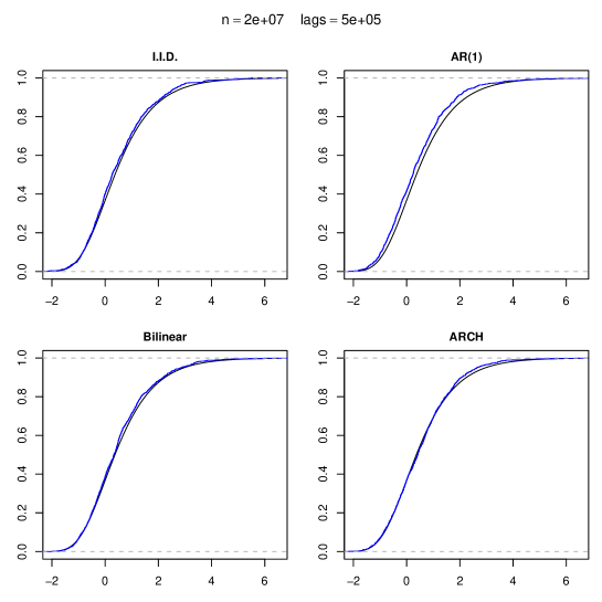
Figure 1: Empirical distribution functions for quantities in (29). We choose $b=0.5$ for model (26), $a=b=0.4$ for model (27), and $a=b=0.25$ for model (28). The black line gives the true distribution function of the Gumbel distribution.

One the other hand, these empirical distributions are not very close to the limiting one if the sample size is not large, because the Gumbel type of convergence in (14) is slow. This is a well-known phenomenon; see for example Hall (1979). It is therefore not reasonable to use the limiting distribution to approximate the finite sample distributions. To perform the test (24), we repeat the BOB procedure as described in Horowitz et al. (2006) (called SBOB in their paper). Since in the bootstrapped tests, the test statistics are not to be compared with the limiting distribution, we can ignore the norming constants in (29) and simply use the following test statistics

$$M_{n}=\max_{1\leq k\leq s_{n}}\left|r_{k}-(1-k/n)r_{k}^{(0)}\right|\mbox{ and }\mathcal{M}_{n}={{M_{n}}\over{\sqrt{\hat{\sigma}_{0}}}},$$

where $\mathcal{M}_{n}$ is the self-normalized version with $\sigma_{0}$ estimated as $\hat{\sigma}_{0}=\sum_{k=-t_{n}}^{t_{n}}\hat{r}_{k}^{2}$, with $t_{n}=\min\{\lfloor n^{1/3}\rfloor,s_{n}\}$. For simplicity, we refer these two tests as $M$-test and $\mathcal{M}$-test, respectively.

From the series $X_{1},\ldots,X_{n}$, for some specified number of lags $s_{n}$ that will be included in the test and block size $\mathfrak{b}_{n}$, form $Y_{i}=(X_{i},X_{i+1},\ldots,X_{i+s_{n}})^{\top}$, $1\leq i\leq n-s_{n}$ and blocks $\mathcal{B}_{j}=(Y_{j},Y_{j+1},\ldots,Y_{j+\mathfrak{b}_{n}-1})$, $1\leq j\leq n-s_{n}-\mathfrak{b}_{n}+1$. For simplicity assume $h_{n}=n/\mathfrak{b}_{n}$ is an integer. Suppose $Y_{\sharp}$ is obtained by sampling a block $\mathcal{B}_{\sharp}$ from the set of blocks $\{\mathcal{B}_{1},\mathcal{B}_{2},\ldots,\mathcal{B}_{n-s_{n}-\mathfrak{b}_{n}+1}\}$, and then sampling a column from $\mathcal{B}_{\sharp}$, let $\operatorname{Cov}_{\sharp}$ represent the covariance of the bootstrap distribution of $Y_{\sharp}$, conditional on $(X_{1},X_{2},\ldots,X_{n})$. Denote by $Y_{\sharp}^{j}$ the $j$-th entry of $Y_{\sharp}$, set

$$r_{k}^{(e)}={{\operatorname{Cov}_{\sharp}(Y_{\sharp}^{1},Y_{\sharp}^{k+1})}\over\sqrt{\operatorname{Cov}_{\sharp}(Y_{\sharp}^{1},Y_{\sharp}^{1})\cdot\operatorname{Cov}_{\sharp}(Y_{\sharp}^{k+1},Y_{\sharp}^{k+1})}}.$$

The explicit formula of $r_{k}^{(e)}$ was also given in Horowitz et al. (2006). The BOB algorithm is as follows.

1. Sample $h_{n}$ times with replacement from $\{\mathcal{B}_{1},\mathcal{B}_{2},\ldots,\mathcal{B}_{n-s_{n}-\mathfrak{b}_{n}+1}\}$ to obtain blocks $\{\mathcal{B}^{\ast}_{1},\mathcal{B}^{\ast}_{2},\,\ldots,\,\mathcal{B}^{\ast}_{h_{n}}\}$, which are laid end-to-end to form a series of vectors $(Y^{\ast}_{1},Y^{\ast}_{2},\ldots,Y^{\ast}_{n})$.

2. Pretend that $(Y^{\ast}_{1},Y^{\ast}_{2},\ldots,Y^{\ast}_{n})$ is a random sample of size $n$ from some $s_{n}$-dimensional population distribution, let $r^{\ast}_{k}$ be the sample correlation of the first entry and the $(k+1)$-th entry. Then calculate the test statistic $M_{n}^{\ast}=\max_{1\leq k\leq s_{n}}\left|r^{\ast}_{k}-r^{(e)}_{k}\right|$ and $\mathcal{M}_{n}^{\ast}=M_{n}^{\ast}/\sqrt{\sigma_{0}^{\ast}}$, where $\sigma_{0}^{\ast}=\sum_{k=-t_{n}}^{t_{n}}\left(r_{k}^{\ast}\right)^{2}$.

3. Repeat steps 1 and 2 for $N$ times. The bootstrap $p$-value of the $M$-test is given by $\#(M_{n}^{\ast}>M_{n})/N$. For a nominal level $\alpha$, we reject $\boldsymbol{\mathrm{H}}_{0}$ if $\#(M_{n}^{\ast}>M_{n})/N<\alpha$. The $\mathcal{M}$-test is performed in the same manner.

We compare the BOB tests and the asymptotic tests for the four models listed at the beginning of this section, with $a=.4$ for (26), $a=b=.4$ for (27) and $a=b=.25$ for (28). We set the series length as $n=1800$, and consider four choices of $s_{n}$: $\lfloor\log(n)\rfloor=7$, $\lfloor n^{1/3}\rfloor=12$, $\lfloor\sqrt{n}\rfloor=42$ and 25. The BOB tests are performed with $N=999$, and the asymptotic tests are carried out by comparing $a_{2s_{n}}^{-1}(\sqrt{n}\mathcal{M}_{n}-b_{2s_{n}})$ with the corresponding quantiles of the Gumbel distribution. The empirical rejection probabilities based on 10,000 repetitions are reported in Table LABEL:tab:sbob. All probabilities are given in percentages. For all cases, we see that the asymptotic tests are too conservative, and the ERP are quite large. At the nominal level $1\%$, the rejection probabilities are often less than or around $0.1\%$, and at most $0.51\%$; while at nominal level $10\%$, they are often less than $3\%$ and at most $6.4\%$. Except for the bilinear models with $s_{n}=7$ and $s_{n}=12$, the bootstrapped tests significantly reduce the ERP, which are often less than $0.2\%$ at nominal level $1\%$, less than $.5\%$ at level $5\%$, and less than $1\%$ at level $10\%$. The performance of $M$-test and $\mathcal{M}$-test are similar, with the former being slightly more conservative. The BOB tests are roughly insensitive to the block size, which provides additional evidence of the findings on BOB tests in Davison and Hinkley (1997).

[ caption = Empirical rejection probabilities (in percentages), label = tab:sbob, pos = ht, ]lrrrcrrrcrrrcrrr []The values 1, 5, 10 in the 2nd row indicate nominal levels in percentages. The numbers in the third row starting with the model name “I.I.D.” are for the asymptotic tests. The fourth row staring with $\mathfrak{b}_{n}=5$ is for BOB $M$-tests with block size 5. The fifth row is for BOB $\mathcal{M}$-tests with the same block size 5. Other rows should be read similarly. Test $s_{n}=7$ $s_{n}=12$ $s_{n}=25$ $s_{n}=42$
1 5 10 1 5 10 1 5 10 1 5 10
I.I.D. .00 .34 1.6 .02 .69 2.3 .03 .93 3.2 .04 1.0 3.3
$\mathfrak{b}_{n}=5$ 1.3 5.1 10.0 1.1 5.2 9.8 .95 4.7 9.3 1.0 4.7 9.6
1.4 5.3 10.4 1.2 5.6 10.5 1.1 5.1 10.1 1.1 5.1 10.2
$\mathfrak{b}_{n}=10$ .83 4.8 10.0 1.1 4.9 9.6 1.1 4.9 10.1 .65 4.3 8.9
.94 5.1 10.3 1.2 5.4 10.3 1.1 5.5 11.0 .78 4.7 9.6
AR(1) .01 .17 1.2 .01 .36 1.8 .02 .77 2.5 .02 .88 2.8
$\mathfrak{b}_{n}=10$ 1.3 5.7 10.9 1.3 5.5 11.4 1.3 5.5 10.9 1.1 5.7 11.2
1.3 5.7 11.2 1.4 5.9 11.7 1.3 6.0 11.5 1.2 6.0 11.7
$\mathfrak{b}_{n}=20$ .98 5.5 10.9 1.0 5.8 11.3 1.1 5.3 10.6 .86 4.9 10.5
1.0 5.7 11.0 1.1 6.1 11.9 1.2 5.6 11.0 .83 5.0 10.9
Bilinear .34 2.8 6.4 .43 2.5 5.8 .51 2.5 5.9 .40 2.8 5.9
$\mathfrak{b}_{n}=10$ 2.8 8.7 14.4 1.8 7.1 12.7 1.2 6.1 12.0 1.2 5.4 10.9
2.7 8.6 14.5 1.8 7.3 12.9 1.3 6.2 12.2 1.1 5.5 11.1
$\mathfrak{b}_{n}=20$ 2.7 8.4 14.6 2.1 7.2 13.5 1.5 6.3 12.0 1.3 5.2 10.8
2.5 8.3 14.6 2.1 7.5 13.9 1.5 6.2 12.0 1.2 5.3 10.9
ARCH .05 .82 3.2 .06 1.5 3.9 .09 1.3 4.0 .12 1.4 4.4
$\mathfrak{b}_{n}=10$ .99 5.0 10.5 1.2 4.9 9.7 .80 4.6 9.9 .82 4.7 9.3
1.1 5.4 10.9 1.4 5.3 10.4 .92 5.1 10.7 .94 5.1 10.2
$\mathfrak{b}_{n}=20$ .86 5.1 10.5 1.0 5.0 10.3 .69 4.8 9.7 .63 4.3 8.9
.98 5.5 11.0 1.2 5.6 11.0 .89 5.1 10.4 .76 4.7 9.5

The bootstrapped tests still perform relatively poorly for bilinear models when $s_{n}$ is small (7 and 12). This is possibly due to the heavy-tailedness of the bilinear process. Tong (1981) gave necessary conditions for the existence of even order moments. On the other hand, Horowitz et al. (2006) showed that the iterated bootstrapping further reduce the ERP. It is of interest to see whether the iterated procedure has the same effect for the ${\cal L}^{\infty}$ based tests, in particular, whether it makes the ERP reasonably small for the bilinear models when $s_{n}$ is small. The simulation for the iterated bootstrapping will be computationally expensive and we do not pursue it here.

4 Proofs

This section provides proofs for the results in Section 2. For readability we list the notation here. For a random variable $X$, write that $X\in\mathcal{L}^{p}$, $p>0$, if $\|X\|_{p}:=(\mathbb{E}|X|^{p})^{1/p}<\infty$. Write $\|X\|=\|X\|_{2}$ if $p=2$. To express centering of random variables concisely, we define the operator $\mathbb{E}_{0}$ as $\mathbb{E}_{0}X:=X-\mathbb{E}X$. For a vector $\boldsymbol{x}=(x_{1},\ldots,x_{d})^{\top}\in\mathbb{R}^{d}$, let $|\boldsymbol{x}|$ be the usual Euclidean norm, $|\boldsymbol{x}|_{\infty}:=\max_{1\leq i\leq d}|x_{i}|$, and $|\boldsymbol{x}|_{\bullet}:=\min_{1\leq i\leq d}|x_{i}|$. For a square matrix $A$, $\rho(A)$ denotes the operator norm defined by $\rho(A):=\max_{|\boldsymbol{x}|=1}|A\boldsymbol{x}|$. Let us make some convention on the constants. We use $C$, $c$ and $\mathcal{C}$ for constants. The notation $\mathcal{C}_{p}$ is reserved for the constant appearing in Burkholder’s inequality, see (31). The values of $C$ may vary from place to place, while the value of $c$ is fixed within the statement and the proof of a theorem (or lemma). A constant with a symbolic subscript is used to emphasize the dependence of the value on the subscript.

The framework (9) is particularly suited for two classical tools for dealing with dependent sequences, martingale approximation and $m$-dependence approximation. For $i\leq j$, define $\mathcal{F}_{i}^{j}=\langle\epsilon_{i},\epsilon_{i+1},\ldots,\epsilon_{j}\rangle$ be the $\sigma$-field generated by the innovations $\epsilon_{i},\epsilon_{i+1},\ldots,\epsilon_{j}$, and the projection operator $\mathcal{H}_{i}^{j}(\cdot)=\mathbb{E}(\cdot|\mathcal{F}_{i}^{j})$. Set $\mathcal{F}_{i}:=\mathcal{F}_{i}^{\infty}$, $\mathcal{F}^{j}:=\mathcal{F}_{-\infty}^{j}$, and define $\mathcal{H}_{i}$ and $\mathcal{H}^{j}$ similarly. Define the projection operator $\mathcal{P}^{j}(\cdot)=\mathcal{H}^{j}(\cdot)-\mathcal{H}^{j-1}(\cdot)$, and $\mathcal{P}_{i}(\cdot)=\mathcal{H}_{i}(\cdot)-\mathcal{H}_{i+1}(\cdot)$, then $(\mathcal{P}^{j}(\cdot))_{j\in\mathbb{Z}}$ and $(\mathcal{P}_{-i}(\cdot))_{i\in\mathbb{Z}}$ become martingale difference sequences with respect to the filtrations $(\mathcal{F}^{j})$ and $(\mathcal{F}_{-i})$, respectively. For $m\geq 0$, define $\tilde{X}_{i}=\mathcal{H}_{i-m}X_{i}$, then $(\tilde{X}_{i})_{i\in\mathbb{Z}}$ is a $(m+1)$-dependent sequence.

4.1 Some Useful Inequalities

We collect in Proposition 8 some useful facts about physical dependence measures and martingale and $m$-dependence approximations. We expect that it will be useful in other asymptotic problems that involve sample covariances. Hence for convenience of other researchers, we provide explicit upper bounds.

We now introduce a moment inequality (30) which follows from the Burkholder inequality (see Burkholder, 1988). Let $(D_{i})$ be a martingale difference sequence and for every $i$, $D_{i}\in\mathcal{L}^{p}$, $p>1$, then

$$\left\|D_{1}+D_{2}+\cdots+D_{n}\right\|_{p}^{p^{\prime}}\leq\mathcal{C}_{p}^{p^{\prime}}\left(\|D_{1}\|_{p}^{p^{\prime}}+\|D_{2}\|_{p}^{p^{\prime}}+\cdots+\|D_{n}\|_{p}^{p^{\prime}}\right),$$ (30)

where $p^{\prime}=\min\{p,2\},$ and the constant

$$\mathcal{C}_{p}=(p-1)^{-1}\hbox{ if }1<p<2\mbox{ and }=\sqrt{p-1}\hbox{ if }p\geq 2.$$ (31)

We note that when $p>2$, the constant $\mathcal{C}_{p}$ in (30) equaled to $p-1$ in Burkholder (1988), and it was improved to $\sqrt{p-1}$ by Rio (2009).

Proposition 8.

1. Assume $\mathbb{E}X_{i}=0$ and $p>1$. Recall that $p^{\prime}=\min(p,2)$.

   $$\|\mathcal{P}^{0}X_{i}\|_{p}\leq\delta_{p}(i)\quad\hbox{and}\quad\|\mathcal{P}_{0}X_{i}\|_{p}\leq\delta_{p}(i)$$ (32)

   $$\kappa_{p}:=\|X_{0}\|_{p}\leq\mathcal{C}_{p}\Psi_{p}$$ (33)

   $$\left\|\sum_{i=1}^{n}c_{i}X_{i}\right\|_{p}\leq\mathcal{C}_{p}A_{n}\Theta_{p},\mbox{ where }A_{n}=\left(\sum_{i=1}^{n}|c_{i}|^{p^{\prime}}\right)^{1/p^{\prime}}$$ (34)

   $$|\gamma_{k}|\leq\zeta_{2}(k),\quad\hbox{where }\zeta_{p}(k):=\sum_{j=0}^{\infty}\delta_{p}(j)\delta_{p}(j+k)$$ (35)

   $$\left\|\sum_{i=1}^{n}(X_{i-k}X_{i}-\gamma_{k})\right\|_{p/2}\leq 2\mathcal{C}_{p/2}\kappa_{p}\Theta_{p}\sqrt{n},\quad\hbox{when }p\geq 4$$ (36)

   $$\left\|\sum_{i,j=1}^{n}c_{i,j}(X_{i}X_{j}-\gamma_{i-j})\right\|_{p/2}\leq 4\mathcal{C}_{p/2}\mathcal{C}_{p}\Theta_{p}^{2}B_{n}\sqrt{n},\quad\hbox{when }p\geq 4$$ (37)

   where $B_{n}^{2}=\max\{\max_{1\leq i\leq n}\sum_{j=1}^{n}c_{i,j}^{2},\,\max_{1\leq j\leq n}\sum_{i=1}^{n}c_{i,j}^{2}\}.$

2. For $m\geq 0$, define $\tilde{X}_{i}=\mathcal{H}_{i-m}X_{i}$. For $p>1$, let $\tilde{\delta}_{p}(\cdot)$ be the physical dependence measures for the sequence $(\tilde{X}_{i})$. Then

   $$\tilde{\delta}_{p}(i)\leq\delta_{p}(i)$$ (38)

   $$\|X_{0}-\tilde{X}_{0}\|_{p}\leq\mathcal{C}_{p}\Psi_{p}(m+1)$$ (39)

   $$\left\|\sum_{i=1}^{n}c_{i}(X_{i}-\tilde{X}_{i})\right\|_{p}\leq\mathcal{C}_{p}A_{n}\Theta_{p}(m+1)$$ (40)

   $$\left\|\sum_{i=k+1}^{n}\left(X_{i-k}X_{i}-\gamma_{k}-\tilde{X}_{i-k}\tilde{X}_{i}+\tilde{\gamma}_{k}\right)\right\|_{p}\leq 4\mathcal{C}_{p}(n-k)^{1/p^{\prime}}\kappa_{2p}\Delta_{2p}(m+1).$$ (41)

Proof.

The inequalities (32) and (38) are obtained by the first principle. Since $X_{i-k}=\sum_{j\in\mathbb{Z}}\mathcal{P}^{j}X_{i-k}$ and $X_{i}=\sum_{j\in\mathbb{Z}}\mathcal{P}^{j}X_{i}$, we have

$$|\gamma_{k}|=\left|\sum_{j=-k}^{\infty}\mathbb{E}\left[(\mathcal{P}^{-j}X_{0})(\mathcal{P}^{-j}X_{k})\right]\right|\leq\delta_{2}(j)\delta_{2}(j+k)\leq\zeta_{k},$$

which proves (35). For (37), it can be similarly proved as Proposition 1 of Liu and Wu (2010), and (40) was given by Lemma 1 of the same paper. (34) is a special case of (40). Define $Y_{i}=X_{i-k}X_{i}$, then $(Y_{i})$ is also a stationary process of the form (9). By Hölder’s inequality, $\|Y_{i}-\Omega_{0}(Y_{i})\|_{p/2}\leq 2\kappa_{p}[\delta_{p}(i)+\delta_{p}(i-k)]$. Applying (34) to $(Y_{i})$, we obtain (36). To see (39), we first write $X_{m}-\tilde{X}_{m}=\sum_{j=1}^{\infty}\mathcal{P}_{-j}X_{m}$. Since $\left\|\mathcal{P}_{-j}X_{m}\right\|_{p}\leq\delta_{p}(m+j)$, and $(\mathcal{P}_{-j}X_{m})_{j\geq 1}$ is a martingale difference sequence, by (30), we have

$$\|X_{0}-\tilde{X}_{0}\|^{p^{\prime}}_{p}\leq\mathcal{C}_{p}^{p^{\prime}}\sum_{j=1}^{\infty}\left\|\mathcal{P}_{-j}X_{m}\right\|_{p}^{p^{\prime}}\leq\mathcal{C}_{p}^{p^{\prime}}\sum_{j=1}^{\infty}[\delta_{p}(m+j)]^{p^{\prime}}=\mathcal{C}_{p}^{p^{\prime}}[\Psi_{p}(m+1)]^{p^{\prime}}.$$

The above argument also leads to (33). Using a similar argument as in the proof of Theorem 2 of Wu (2009), we can show (41). Details are omitted. ∎

4.2 Proof of Theorem 1

The proof is quite complicated and will be divided into several steps. We first give the outline.

4.1.0. Outline

Step 1: $m$-dependence approximation.

Define $R_{n,k}=\sum_{i=k+1}^{n}(X_{i-k}X_{i}-\gamma_{k})$. Set $m_{n}=\lfloor n^{\beta}\rfloor$, $0<\beta<1$. Define $\tilde{X}_{i}=\mathcal{H}_{i-m_{n}}X_{i}$, $\tilde{\gamma}_{k}=\mathbb{E}(\tilde{X}_{0}\tilde{X}_{k})$, and $\tilde{R}_{n,k}=\sum_{i=k+1}^{n}(\tilde{X}_{i-k}\tilde{X}_{i}-\tilde{\gamma}_{k})$. We next show that it suffices to consider $\tilde{R}_{n,k}$.

Lemma 9.

Assume $\mathbb{E}X_{i}=0$, $X_{i}\in\mathcal{L}^{p}$, and $\Theta_{p}(m)=O(m^{-\alpha})$ for some $p>4$ and $\alpha>0$. If $s_{n}=O(n^{\eta})$ with $0<\eta<\alpha p/2$, then there exists a $\beta$ such that $\eta<\beta<1$ and

$$\max_{1\leq k\leq s_{n}}\left|R_{n,k}-\tilde{R}_{n,k}\right|=o_{P}\left(\sqrt{n/\log s_{n}}\right).$$

Step 2: Throw out small blocks.

Let $l_{n}=\lfloor n^{\gamma}\rfloor$, where $\gamma\in(\beta,1)$. For each $t_{n}<k\leq s_{n}$, we apply the blocking technique and split the integer interval $[k+1,n]$ into alternating large and small blocks

$$K_{1}=[k+1,s_{n}]$$ (42)

$$H_{j}=[s_{n}+(j-1)(2m_{n}+l_{n})+1,s_{n}+(j-1)(2m_{n}+l_{n})+l_{n}];\quad 1\leq j\leq w_{n}-1,$$

$$K_{j+1}=[s_{n}+(j-1)(2m_{n}+l_{n})+l_{n}+1,s_{n}+j(2m_{n}+l_{n})];\quad 1\leq j\leq w_{n}-1;\quad\hbox{and}$$

$$H_{w_{n}}=[s_{n}+(w_{n}-1)(2m_{n}+l_{n})+1,n],$$

where $w_{n}$ is the largest integer such that $s_{n}+(w_{n}-1)(2m_{n}+l_{n})+l_{n}\leq n$. Denote by $|H|$ the size of a block $H$. By definition we know $l_{n}\leq|H_{w_{n}}|\leq 3l_{n}$ when $n$ is large enough. For $1\leq j\leq w_{n}$ define

$$V_{k,j}=\sum_{i\in K_{j},\,i>k}\left(\tilde{X}_{i-k}\tilde{X}_{i}-\tilde{\gamma}_{k}\right)\mbox{ and }U_{k,j}=\sum_{i\in H_{j}}\left(\tilde{X}_{i-k}\tilde{X}_{i}-\tilde{\gamma}_{k}\right).$$

Note that $w_{n}\sim n/(2m_{n}+l_{n})\sim n^{1-\gamma}$. We show that the sums over small blocks are negligible.

Lemma 10.

Assume the conditions of Theorem 1. Then

$$\max_{1\leq k\leq s_{n}}\left|\sum_{j=1}^{w_{n}}V_{k,j}\right|=o_{P}\left(\sqrt{\frac{n}{\log s_{n}}}\right).$$

Step 3: Truncate sums over large blocks.

We show that it suffices to consider

$$\mathcal{R}_{n,k}=\sum_{j=1}^{w_{n}}\bar{U}_{k,j},\mbox{ where }\bar{U}_{k,j}=\mathbb{E}_{0}\left(U_{k,j}I\{|U_{k,j}|\leq\sqrt{n}/(\log s_{n})^{3}\}\right).$$

Lemma 11.

Assume the conditions of Theorem 1. Then

$$\max_{1\leq k\leq s_{n}}\left|\sum_{j=1}^{w_{n}}(U_{k,j}-\bar{U}_{k,j})\right|=o_{P}\left(\sqrt{\frac{n}{\log s_{n}}}\right).$$

Step 4: Compare covariance structures.

In order to prove Lemma 14, we need the autocovariance structure of $\left(\mathcal{R}_{n,k}/\sqrt{n}\right)$ to be close to that of $(G_{k})$. However, this only happens when $k$ is large. We show that there exists an $0<\iota<1$ such that for $t_{n}=3\lfloor s_{n}^{\iota}\rfloor$, (i) $\max_{1\leq k\leq t_{n}}|\mathcal{R}_{n,k}/\sqrt{n}|$ does not contribute to the asymptotic distribution; and (ii) the autocovariance structure of $\left(\mathcal{R}_{n,k}/\sqrt{n}\right)$ converges to that of $(G_{k})$ uniformly on $t_{n}<k\leq s_{n}$.

Lemma 12.

Under conditions of Theorem 1, there exists a constant $0<\iota<1$ such that for $t_{n}=3\lfloor s_{n}^{\iota}\rfloor$,

$$\lim_{n\to\infty}P\left(\max_{1\leq k\leq t_{n}}|\mathcal{R}_{n,k}|>\sqrt{\sigma_{0}n\log s_{n}}\right)=0.$$ (43)

Lemma 13.

Let conditions of Theorem 1 be satisfied. Recall that $t_{n}=3\lfloor s_{n}^{\iota}\rfloor$ from Lemma 12. There exist constants $C_{p}>0$ and $0<\ell<1$ such that for any $t_{n}<k\leq k+h\leq s_{n}$,

$$|\operatorname{Cov}(\mathcal{R}_{n,k},\mathcal{R}_{n,k+h})/n-\sigma_{h}|\leq C_{p}\,s_{n}^{-\ell}.$$

Step 5: Moderate deviations.

Let $t_{n}=3\lfloor s_{n}^{\iota}\rfloor$ be as in Lemma 12. For $t_{n}<k_{1}<k_{2}<\ldots<k_{d}\leq s_{n}$, define $\boldsymbol{\mathcal{R}}_{n}=(\mathcal{R}_{n,k_{1}},\mathcal{R}_{n,k_{2}},\ldots,\mathcal{R}_{n,k_{d}})^{\top}$ and $\boldsymbol{V}=(G_{k_{1}},G_{k_{2}},\ldots,G_{k_{d}})^{\top}$, where $(G_{k})$ is defined in (6). Let $\Sigma_{n}=\operatorname{Cov}(\boldsymbol{\mathcal{R}}_{n})$ and $\Sigma=\operatorname{Cov}(\boldsymbol{V})$. For fixed $x\in\mathbb{R}$, set $z_{n}=a_{2s_{n}}x+b_{2s_{n}}$, where the constants $a_{n}$ and $b_{n}$ are defined in (7). In the following lemma we provide a moderate deviation result for $\boldsymbol{\mathcal{R}}_{n}$.

Lemma 14.

Assume conditions of Theorem 1. Then there exists a constant $C_{p,d}>1$ such that for all $t_{n}<k_{1}<k_{2}<\ldots<k_{d}\leq s_{n}$,

$$\left|P\left(\left|\boldsymbol{\mathcal{R}}_{n}/\sqrt{n}\right|_{\bullet}\geq z_{n}\right)-P\left(\left|\boldsymbol{V}\right|_{\bullet}\geq z_{n}\right)\right|\leq C_{p,d}{{P\left(\left|\boldsymbol{V}\right|_{\bullet}\geq z_{n}\right)}\over{(\log s_{n})^{1/2}}}+C_{p,d}\,\exp\left\{-{{(\log s_{n})^{2}}\over{C_{p,d}}}\right\}.$$

4.2.1 Step 1: $m$-dependence approximation

Proof of Lemma 9.

Recall that $m_{n}=\lfloor n^{\beta}\rfloor$ with $\eta<\beta<1$. We claim

$$\left\|R_{n,k}-\tilde{R}_{n,k}\right\|_{p/2}\leq 6\,\mathcal{C}_{p/2}\Theta_{p}\Theta_{p}(m_{n}-k+1)\cdot\sqrt{n}.$$ (44)

It follows that for any $\lambda>0$

$$P \left(\max_{1\leq k\leq s_{n}}\left|R_{n,k}-\tilde{R}_{n,k}\right|>\lambda\sqrt{n/\log s_{n}}\right)\leq{{(\log s_{n})^{p/4}}\over{n^{p/4}\lambda^{p/2}}}\sum_{k=1}^{s_{n}}\|R_{n,k}-\tilde{R}_{n,k}\|^{p/2}_{p/2}$$

$$\qquad\qquad\qquad\leq C_{p}\lambda^{-p/2}s_{n}(\log s_{n})^{p/4}n^{-\alpha\beta p/2}\leq C_{p}\lambda^{-p/2}n^{\eta-\alpha\beta p/2}(\log n)^{p/4}.$$

Therefore, if $\alpha p/2>\eta$, then there exists a $\beta$ such that $\eta<\beta<1$ and $\eta-\alpha\beta p/2<0$, and hence the preceding probability goes to zero as $n\to\infty$. The proof of Lemma 9 is complete.

We now prove claim (44). For each $1\leq k\leq s_{n}$, we have

$$\|R_{n,k}-\tilde{R}_{n,k}\|_{p/2}\leq \left\|\sum_{i=k+1}^{n}(X_{i-k}-\tilde{X}_{i-k})\tilde{X}_{i}\right\|_{p/2}+\left\|\sum_{i=k+1}^{n}(\mathcal{H}_{i-m_{n}}X_{i-k})(X_{i}-\tilde{X}_{i})\right\|_{p/2}$$

$$+\left\|\sum_{i=k+1}^{n}\mathbb{E}_{0}\left[(X_{i-k}-\mathcal{H}_{i-m_{n}}X_{i-k})(X_{i}-\tilde{X}_{i})\right]\right\|_{p/2}$$

Observe that $(\tilde{X}_{i}\mathcal{P}_{i-k-j}X_{i-k})_{1\leq i\leq n}$ is a backward martingale difference sequence with respect to $\mathcal{F}_{i-k-j}$ if $j>m_{n}$, so by the inequality (30),

$$\left\|\sum_{i=k+1}^{n}(X_{i-k}-\tilde{X}_{i-k})\tilde{X}_{i}\right\|_{p/2} \leq\sum_{j=m+1}^{\infty}\left\|\sum_{i=k+1}^{n}\tilde{X}_{i}\mathcal{P}_{i-k-j}X_{i-k}\right\|_{p/2}$$

$$\leq\sum_{j=m+1}^{\infty}\sqrt{n}\mathcal{C}_{p/2}\|\tilde{X}_{j+k}\mathcal{P}_{0}X_{j}\|_{p/2}$$

$$\leq\mathcal{C}_{p/2}\Theta_{p}\Theta_{p}(m_{n}+1)\cdot\sqrt{n}.$$

Similarly we have $\|\sum_{i=k+1}^{n}(\mathcal{H}_{i-m_{n}}X_{i-k})(X_{i}-\tilde{X}_{i})\|_{p/2}\leq\sqrt{n}\mathcal{C}_{p/2}\Theta_{p}\Theta_{p}(m_{n}+1)$. Similarly as (40), we get $\|\tilde{X}_{i-k}-\mathcal{H}_{i-m_{n}}X_{i-k}\|_{p}\leq\Theta_{p}(m_{n}-k+1)$. Let $Y_{n,i}:=(X_{i-k}-\mathcal{H}_{i-m_{n}}X_{i-k})(X_{i}-\tilde{X}_{i})$. Then

$$\left\|Y_{n,i}-\Omega_{0}(Y_{n,i})\right\|_{p/2}\leq 2\left[\delta_{p}(i)\Theta_{p}(m_{n}-k+1)+\delta_{p}(i-k)\Theta_{p}(m_{n}+1)\right].$$

Therefore, by (34), it follows that

$$\left\|\sum_{i=k+1}^{n}\mathbb{E}_{0}\left[(X_{i-k}-\mathcal{H}_{i-m_{n}}X_{i-k})(X_{i}-\tilde{X}_{i})\right]\right\|_{p/2}\leq 4\,\mathcal{C}_{p/2}\Theta_{p}\Theta_{p}(m_{n}-k+1)\cdot\sqrt{n},$$

and the proof of (44) is complete. ∎

4.2.2 Step 2: Throw out small blocks

In this section, as well as many other places in this article, we often need to split an integer interval $[s,t]=\{s,s+1,\ldots,t\}\subset\mathbb{N}$ into consecutive blocks $\mathcal{B}_{1},\ldots,\mathcal{B}_{w}$ with the size $m$. Since $s-t+1$ may not be a multiple of $m$, we make the convention that unless the size of the last block is specified clearly, it has the size $m\leq|\mathcal{B}_{w}|<2m$, and all the other ones have the same size $m$.

Proof of Lemma 10.

It suffices to show that for any $\lambda>0$,

$$\lim_{n\to\infty}\sum_{k=1}^{s_{n}}P\left(\left|\sum_{j=1}^{w_{n}}V_{k,j}\right|\geq\lambda\sqrt{\frac{n}{\log s_{n}}}\right)=0.$$

Observe that $V_{k,j},1\leq j\leq w_{n}$, are independent. By (36), $\|V_{k,j}\|\leq 2|K_{j}|^{1/2}\kappa_{4}\Theta_{4}$. By Corollary 1.6 of Nagaev (1979), for any $M>1$, there exists a constant $C_{M}>1$ such that

$$P\left(\left|\sum_{j=1}^{w_{n}}V_{k,j}\right|\geq\lambda\sqrt{\frac{n}{\log s_{n}}}\right) \leq\sum_{j=1}^{w_{n}}P\left(|V_{k,j}|\geq C_{M}^{-1}\lambda\sqrt{{n}/{\log s_{n}}}\right)+\left(\frac{4e^{2}\kappa_{4}^{2}\Theta_{4}^{2}\sum_{j=1}^{w_{n}}|K_{j}|}{C_{M}^{-1}\lambda^{2}n/\log s_{n}}\right)^{C_{M}/2}$$ (45)

$$\leq\sum_{j=1}^{w_{n}}P\left(|V_{k,j}|\geq C_{M}^{-1}\lambda\sqrt{{n}/{\log n}}\right)+C_{M}\left(n^{\beta-\gamma}\log n\right)^{C_{M}/2}$$

$$\leq\sum_{j=1}^{w_{n}}P\left(|V_{k,j}|\geq C_{M}^{-1}\sqrt{{n}/{\log n}}\right)+n^{-M}.$$

where we resolve the constant $\lambda$ into the constant $C_{M}$ in the last inequality. It remains to show that

$$\lim_{n\to\infty}\sum_{k=1}^{s_{n}}\sum_{j=1}^{w_{n}}P\left(|V_{k,j}|\geq q_{1}\delta\phi_{n}\right)=0,\mbox{ where }\phi_{n}=\sqrt{\frac{n}{\log n}},$$ (46)

holds for any $\delta>0$, where $q_{1}$ is the smallest integer such that $\beta^{q_{1}}<\min\{(p-4)/p,\,(p-2-2\eta)/(p-2)\}$. This choice of $q_{1}$ will be explained later. We adopt the technique of successive $m$-dependence approximations from Liu and Wu (2010) to prove (46).

For $q\geq 1$, set $m_{n,q}=\lfloor n^{\beta^{q}}\rfloor$. Define $X_{i,q}=\mathcal{H}_{i-m_{n,q}}X_{i}$, $\gamma_{k,q}=\mathbb{E}(X_{0,q}X_{k,q})$, and

$$V_{k,j,q}=\sum_{i\in K_{j},i>k}(X_{i-k,q}X_{i,q}-\gamma_{k,q}).$$

In particular, $m_{n,1}$ is same as $m_{n}$ defined in Step 2, and $V_{k,j,1}=V_{k,j}$. Without loss of generality assume $s_{n}\leq\lfloor n^{\eta}\rfloor$. Let $q_{0}$ be such that $\beta^{q_{0}+1}\leq\eta<\beta^{q_{0}}$. We first consider the difference between $V_{k,j,q}$ and $V_{k,j,q+1}$ for $1\leq q<q_{0}$. Split the block $K_{j}$ into consecutive small blocks $\mathcal{B}_{1},\ldots,\mathcal{B}_{w_{n,q}}$ with size $2m_{n,q}$. Define

$$V_{k,j,q,t}^{(0)}=\sum_{i\in\mathcal{B}_{t}}(X_{i-k,q}X_{i,q}-\gamma_{k,q})\quad\hbox{and}\quad V_{k,j,q,t}^{(1)}=\sum_{i\in\mathcal{B}_{t}}(X_{i-k,q+1}X_{i,q+1}-\gamma_{k,q+1}).$$ (47)

Observe that $V_{k,j,q,t_{1}}^{(0)}$ and $V_{k,j,q,t_{2}}^{(0)}$ are independent if $|t_{1}-t_{2}|>1$. Similar as (45), for any $M>1$, there exists a constant $C_{M}>1$ such that, for sufficiently large $n$,

$$P\left(\left|V_{k,j,q}-V_{k,j,q+1}\right|\geq\delta\phi_{n}\right) =P\left[\left|\sum_{t=1}^{w_{n,q}}\left(V^{(0)}_{k,j,q,t}-V^{(1)}_{k,j,q,t}\right)\right|\geq\delta\phi_{n}\right]$$ (48)

$$\leq\sum_{t=1}^{w_{n,q}}P\left(\left|V^{(0)}_{k,j,q,t}-V^{(1)}_{k,j,q,t}\right|\geq C_{M}^{-1}\phi_{n}\right)+n^{-M}.$$

Similarly as (44), we have $\left\|V^{(0)}_{k,j,q,t}-V^{(1)}_{k,j,q,t}\right\|_{p/2}\leq C_{p}|\mathcal{B}_{t}|^{1/2}m_{n,q+1}^{-\alpha}$. It follows that

$$\sum_{k=1}^{s_{n}}\sum_{j=1}^{w_{n}}P\left(\left|V_{k,j,q}-V_{k,j,q+1}\right|\geq\delta\phi_{n}\right) \leq C_{p,M}n^{\eta}n^{1-\gamma}\left(n^{-M}+\frac{n^{\gamma}m_{n,q}^{p/4}m_{n,q+1}^{-\alpha p/2}}{m_{n,q}(n/\log n)^{p/4}}\right)$$

$$\leq C_{p,M}\left(n^{\eta+1-\gamma-M}+n^{\eta}n^{1-p/4}m_{n,q}^{p/4-1-\alpha\beta p/2}\right).$$

Under the condition (17), there exists a $0<\beta<1$, such that

$$\sum_{k=1}^{s_{n}}\sum_{j=1}^{w_{n}}P\left(\left|V_{k,j,q}-V_{k,j,q+1}\right|\geq\delta\phi_{n}\right)\leq C_{p,M}\left(n^{\eta+1-\gamma-M}+n^{\eta+1-p/4+\beta^{q}(p/4-1-\alpha\beta p/2)}\right)\to 0.$$

Recall that $q_{1}$ is the smallest integer such that $\beta^{q_{1}}<\min\{(p-4)/p,(p-2-2\eta)/(p-2)\}$. We now consider the difference between $V_{k,j,q}$ and $V_{k,j,q+1}$ for $q_{0}\leq q<q_{1}$. The problem is more complicated than the preceding case $1\leq q<q_{0}$, since now it is possible that $m_{n,q}<k$ for some $1\leq k\leq s_{n}$. We consider three cases.

Case 1: $k\geq 2m_{n,q}$. Partition the block $K_{j}$ into consecutive smaller blocks $\mathcal{B}_{1},\ldots,\mathcal{B}_{w_{n,q}}$ with same size $m_{n,q}$. Define $V_{k,j,q,t}^{(0)}$ and $V_{k,j,q,t}^{(1)}$ as in (47). Observe that $\left(V_{k,j,q,t}^{(0)}-V_{k,j,q,t}^{(1)}\right)_{t\hbox{ \scriptsize{is odd}}}$ is a martingale difference sequence with respective to the filtration $\left(\xi_{t}:=\langle\epsilon_{l}:\,l\leq\max\left\{\mathcal{B}_{t}\right\}\rangle\right)_{t\hbox{ \scriptsize{is odd}}}$, and so is the sequence and filtration labelled by even $t$. Set $\xi_{0}=\langle\epsilon_{l}:\,l<\min\{\mathcal{B}_{1}\}\rangle$ and $\xi_{-1}=\langle\epsilon_{l}:\,l<\min\{\mathcal{B}_{1}\}-m_{n,q}\rangle$. For each $1\leq t\leq w_{n,q}$, define

$$\mathcal{V}^{(l)}_{t}=\mathbb{E}\left[\left(V^{(l)}_{k,j,q,t}\right)^{2}|\xi_{t-2}\right]=\sum_{i_{1},i_{2}\in\mathcal{B}_{t}}X_{i_{1}-k,q+l}X_{i_{2}-k,q+l}\gamma_{i_{1}-i_{2},q+l}$$

for $l=0,1$. By Lemma 1 of Haeusler (1984), for any $M>1$, there exists a constant $C_{M}>1$ such that

$$P \left(\left|V_{k,j,q}-V_{k,j,q+1}\right|\geq\delta\phi_{n}\right)\leq\sum_{t=1}^{w_{n,q}}P\left(\left|V^{(0)}_{k,j,q,t}-V^{(1)}_{k,j,q,t}\right|\geq\sqrt{\frac{n}{(\log n)^{3}}}\right)+n^{-M}$$ (49)

$$\quad+\sum_{l=0,1}2\left\{P\left[\sum_{t\hbox{ {\scriptsize is odd}}}\mathcal{V}^{(l)}_{t}\geq\frac{C_{M}^{-1}n}{(\log n)^{2}}\right]+P\left[\sum_{t\hbox{ {\scriptsize is even}}}\mathcal{V}^{(l)}_{t}\geq\frac{C_{M}^{-1}n}{(\log n)^{2}}\right]\right\}.$$

By (35), $\sum_{k\in\mathbb{Z}}|\gamma_{k,q+l}|^{2}\leq\Theta_{2}^{2}$, and hence by (37), $\|\mathcal{V}^{(l)}_{t}\|_{p/2}\leq C_{p}m_{n,q}^{1/2}$. Observe that $\mathcal{V}^{(0)}_{t_{1}}$ and $\mathcal{V}^{(0)}_{t_{1}}$ are independent if $|t_{1}-t_{2}|>1$, so similarly as (45), we have

$$P\left[\sum_{t\hbox{ {\scriptsize is odd}}}\mathcal{V}^{(l)}_{t}\geq\frac{C_{M}^{-1}n}{(\log n)^{2}}\right] \leq n^{-M}+\sum_{t\hbox{ {\scriptsize is odd}}}P\left[\mathcal{V}^{(l)}_{t}\geq\frac{C_{M}^{-2}n}{(\log n)^{2}}\right]$$

$$\leq n^{-M}+C_{p,M}\cdot w_{n,q}\cdot n^{-p/2}(\log n)^{p}\cdot m_{n,q}^{p/4}.$$

The same inequality holds for the sum over even $t$. For the first term in (49), we claim that

$$\left\|V^{(0)}_{k,j,q,t}-V^{(1)}_{k,j,q,t}\right\|_{p}\leq C_{p}\cdot m_{n,q}^{1/2}\cdot m_{n,q+1}^{-\alpha},$$ (50)

which together with the preceding two inequalities implies that

$$P \left(\left|V_{k,j,q}-V_{k,j,q+1}\right|\geq\delta\phi_{n}\right)\leq C_{p,M}\,w_{n,q}\cdot n^{-p/2}(\log n)^{3p/2}\left(m_{n,q}^{p/2}\cdot m_{n,q+1}^{-\alpha p}+m_{n,q}^{p/4}\right)+n^{-M}.$$

It follows that under condition (17), there exists a $0<\beta<1$ such that

$$\sum_{k=2m_{n,q}}^{s_{n}}\sum_{j=1}^{w_{n}}P\left(\left|V_{k,j,q}-V_{k,j,q+1}\right|\geq\delta\phi_{n}\right)$$ (51)

$$\quad\leq n^{1+\eta-M}+C_{p,M}\cdot n^{1+\eta-p/2}(\log n)^{3p/2}\left[n^{\beta^{q}(p/2-1-\alpha\beta p)}+n^{\beta^{q}(p/4-1)}\right]=o(1).$$

Case 2: $k\leq m_{n,q+1}/2$. Partition the block $K_{j}$ into consecutive smaller blocks $\mathcal{B}_{1},\ldots,\mathcal{B}_{w_{n,q}}$ with size $3m_{n,q}$. Define $V_{k,j,q,t}^{(0)}$ and $V_{k,j,q,t}^{(1)}$ as in (47). Similarly as (44), we have

$$\left\|V^{(0)}_{k,j,q,t}-V^{(1)}_{k,j,q,t}\right\|_{p/2}\leq C_{p}\cdot m_{n,q}^{1/2}\cdot m_{n,q+1}^{-\alpha}.$$

Similar as (48), for any $M>1$, there exist a constant $C_{M}>1$ such that

$$P\left(\left|V_{k,j,q}-V_{k,j,q+1}\right|\geq\delta\phi_{n}\right) \leq\sum_{t=1}^{w_{n,q}}P\left(\left|V^{(0)}_{k,j,q,t}-V^{(1)}_{k,j,q,t}\right|\geq C_{M}^{-1}\phi_{n}\right)+n^{-M}$$

$$\leq n^{-M}+C_{p,M}\cdot w_{n,q}\cdot n^{-p/4}(\log n)^{p/4}\cdot m_{n,q}^{p/4}\cdot m_{n,q+1}^{-\alpha\beta p/2}.$$

It follows that that under condition (17), there exists a $0<\beta<1$ such that

$$\sum_{k=1}^{m_{n,q+1}/2}\sum_{j=1}^{w_{n}}P\left(\left|V_{k,j,q}-V_{k,j,q+1}\right|\geq\delta\phi_{n}\right)$$ (52)

$$\quad\leq n^{1+\eta-M}+C_{p,M}\cdot n^{1-p/4}(\log n)^{p/4}\cdot\left(n^{\beta^{q}}\right)^{p/4-\alpha\beta p/2}=o(1).$$

Case 3: $m_{n,q+1}/2<k<2m_{n,q}$. We use the same argument as in Case 2. But this time we claim that

$$\left\|V^{(0)}_{k,j,q,t}-V^{(1)}_{k,j,q,t}\right\|_{p/2}\leq C_{p}\left[m_{n,q}^{1/2}\cdot m_{n,q+1}^{-\alpha}+m_{n,q}\zeta_{p}(k)\right],$$ (53)

where $\zeta_{p}(k)$ is defined in (35). Since $\sum_{k=m}^{\infty}[\zeta_{p}(k)]^{p/2}\leq\left[\sum_{k=m}^{\infty}\zeta_{p}(k)\right]^{p/2}=O(m^{-\alpha p/2})$, under condition (13), there exist constants $C_{p,M}>1$ and $0<\beta<1$ such that for $M$ large enough

$$\sum_{k>m_{n,q+1}/2}^{2m_{n,q}-1}\sum_{j=1}^{w_{n}}P\left(\left|V_{k,j,q}-V_{k,j,q+1}\right|\geq\delta\phi_{n}\right)\leq C_{p,M}\cdot n^{1-p/4}(\log n)^{p/4}m_{n,q}^{p/4-\alpha\beta p/2}$$ (54)

$$\qquad+n^{1+\eta-M}+C_{p,M}\cdot n^{1-p/4}(\log n)^{p/4}\cdot m_{n,q}^{p/2-1}\sum_{k>m_{n,q+1}/2}^{2m_{n,q}-1}[\zeta_{p}(k)]^{p/2}$$

$$\quad\leq n^{1+\eta-M}+C_{p,M}\cdot n^{1-p/4}(\log n)^{p/4}\cdot m_{n,q}^{p/2-1-\alpha\beta p/2}=o(1).$$

Alternatively, if we use the bound from (41), $\left\|V^{(0)}_{k,j,q,t}-V^{(1)}_{k,j,q,t}\right\|_{p/2}\leq C_{p}m_{n,q}^{1/2}\cdot m_{n,q+1}^{-\alpha^{\prime}}$, it is still true that under condition (13), there exist constants $C_{p,M}>1$ and $0<\beta<1$ such that for $M$ large enough

$$\sum_{k>m_{n,q+1}/2}^{2m_{n,q}-1} \sum_{j=1}^{w_{n}}P\left(\left|V_{k,j,q}-V_{k,j,q+1}\right|\geq\delta\phi_{n}\right)$$ (55)

$$\leq n^{1+\eta-M}+C_{p,M}\cdot n^{1-p/4}(\log n)^{p/4}\cdot m_{n,q}^{p/2-1-\alpha^{\prime}\beta p/2}=o(1).$$

Combine (51), (52), (54) and (55), we have shown that

$$\lim_{n\to\infty}\sum_{k=1}^{s_{n}}\sum_{j=1}^{w_{n}}P\left(\left|V_{k,j,q}-V_{k,j,q+1}\right|\geq\delta\phi_{n}\right)=0.$$ (56)

for $1\leq q<q_{1}$. Therefore, to prove (46), it suffices to show

$$\lim_{n\to\infty}\sum_{k=1}^{s_{n}}\sum_{j=1}^{w_{n}}P\left(|V_{k,j,q_{1}}|\geq\delta\phi_{n}\right)=0$$ (57)

By considering two cases (i) $2m_{n,q_{1}}\leq k\leq s_{n}$ and (ii) $1\leq k<2m_{n,q_{1}}$ under the condition $\beta^{q_{1}}<\min\{(p-4)/p,(p-2-2\eta)/(p-2)\}$, and using similar arguments as those in proving (56), we can obtain (57). The proof of Lemma 10 is complete.

We now turn to the proof of the two claims (50) and (53). For (53), we have

$$\left\|V^{(0)}_{k,j,q,t}-V^{(1)}_{k,j,q,t}\right\|_{p/2}\leq \left\|\sum_{i\in\mathcal{B}_{t}}(X_{i-k,q}-X_{i-k,q+1})X_{i,q+1}\right\|_{p/2}+\left\|\sum_{i\in\mathcal{B}_{t}}\mathbb{E}_{0}\left[X_{i-k,q+1}(X_{i,q}-X_{i,q+1})\right]\right\|_{p/2}$$

$$+\left\|\sum_{i\in\mathcal{B}_{t}}\mathbb{E}_{0}\left[(X_{i-k,q}-X_{i-k,q+1})(X_{i,q}-X_{i,q+1})\right]\right\|_{p/2}=:I+I\negthinspace I+I\negthinspace I\negthinspace I.$$

Similarly as in the proof of (44), we have

$$I\leq\mathcal{C}_{p/2}\Theta_{p}\Theta_{p}(m_{n,q+1}+1)\cdot\sqrt{3m_{n,q}}\quad\hbox{and}\quad I\negthinspace I\negthinspace I\leq 4\,\mathcal{C}_{p/2}\Theta_{p}\Theta_{p}(m_{n,q+1}+1)\cdot\sqrt{3m_{n,q}}.$$

For the second term $I\negthinspace I$, write

$$\mathbb{E}_{0}\left[X_{i-k,q+1}(X_{i,q}-X_{i,q+1})\right]=\sum_{l_{1}=0}^{m_{n,q+1}}\sum_{l_{2}=m_{n,q+1}+1}^{m_{n,q}}\mathbb{E}_{0}\left[(\mathcal{P}_{i-k-l_{1}}X_{i-k})(\mathcal{P}_{i-l_{2}}X_{i})\right].$$

For a pair $(l_{1},l_{2})$ such that $i-k-l_{1}\neq i-l_{2}$, by the inequality (30), we have

$$\left\|\sum_{i\in\mathcal{B}_{t}}(\mathcal{P}_{i-k-l_{1}}X_{i-k})(\mathcal{P}_{i-l_{2}}X_{i})\right\|_{p/2}\leq\mathcal{C}_{p/2}\delta_{p}(l_{1})\delta_{p}(l_{2})\cdot\sqrt{3m_{n,q}}.$$

For the pairs $(l_{1},l_{2})$ such that $i-k-l_{1}=i-l_{2}$, by the triangle inequality

$$\left\|\sum_{i\in\mathcal{B}_{t}}\sum_{l=0}^{m_{n,q+1}}\mathbb{E}_{0}\left[(\mathcal{P}_{i-k-l}X_{i-k})(\mathcal{P}_{i-k-l}X_{i})\right]\right\|_{p/2}\leq 3m_{n,q}\cdot 2\sum_{l=0}^{m_{n,q+1}}\delta_{p}(l)\delta_{p}(k+l)\leq 6m_{n,q}\zeta_{p}(k).$$

Putting these pieces together, the proof of (53) is complete. The key observation in proving (50) is that since $k\geq 2m_{n,q}$, $X_{i-k,q}$ and $X_{i,q}$ are independent, hence the product $X_{i-k,q}X_{i,q}$ has finite $p$-th moment. The rest of the proof is similar to that of (53). Details are omitted. ∎

Remark 2.

Condition (13) is only used to deal with Case 3, while (17) suffices for the rest of the proof. In fact, for linear processes, one can show that the term $m_{n,q}\zeta_{p}(k)$ in (53) can be removed, so we have (54) under condition (17) and do not need (55). So (17) suffices for Theorem 1. Furthermore, for nonlinear processes with $\delta_{p}(k)=O\left[k^{-(1/2+\alpha)}\right]$, the term $m_{n,q}\zeta_{p}(k)$ can also be removed from (53). Details are omitted.

4.2.3 Step 3: Truncate sums over large blocks

Proof of Lemma 11.

We need to show for any $\lambda>0$

$$\lim_{n\to\infty}\sum_{k=1}^{s_{n}}P\left(\left|\sum_{j=1}^{w_{n}}(U_{k,j}-\bar{U}_{k,j})\right|\geq\lambda\sqrt{\frac{n}{\log s_{n}}}\right)=0.$$

Using (36), elementary calculation gives

$$\left\|{\tilde{U}}_{k,j}-\bar{U}_{k,j}\right\|^{2}\leq\frac{\mathbb{E}|{\tilde{U}}_{k,j}|^{p/2}}{(\sqrt{n}/\log s_{n})^{p/2-2}}\leq\frac{(2\mathcal{C}_{p/2}\kappa_{p}\Theta_{p})^{p/2}|H_{j}|^{p/4}(\log s_{n})^{3(p-4)/2}}{n^{(p-4)/4}}.$$ (58)

Similarly as (45), for any $M>1$, there exists a constant $C_{M}>1$ such that

$$P\left(\left|\sum_{j=1}^{w_{n}}(U_{k,j}-\bar{U}_{k,j})\right|\geq\lambda\sqrt{\frac{n}{\log s_{n}}}\right)\leq \sum_{j=1}^{w_{n}}P\left(|U_{k,j}-\bar{U}_{k,j}|\geq C_{M}^{-1}\lambda\sqrt{\frac{n}{\log s_{n}}}\right)$$

$$+\left(\frac{C_{p}\sum_{j=1}^{w_{n}}|H_{j}|^{p/4}(\log n)^{3p/2}}{C_{M}^{-1}\lambda^{2}n^{p/4}}\right)^{C_{M}/2}$$

$$\leq \sum_{j=1}^{w_{n}}P\left(|U_{k,j}-\bar{U}_{k,j}|\geq C_{M}^{-1}\sqrt{\frac{n}{\log s_{n}}}\right)+n^{-M}.$$

Therefore, it suffices to show that for any $\delta>0$,

$$\lim_{n\to\infty}\sum_{k=1}^{s_{n}}\sum_{j=1}^{w_{n}}P\left(|U_{k,j}-\bar{U}_{k,j}|\geq\delta\sqrt{\frac{n}{\log n}}\right)=0.$$

Since we can use the same arguments as those for (46), Lemma 11 follows. ∎

4.2.4 Step 4: Compare covariance structures

Proof of Lemma 12.

Since $|\bar{U}_{k,j}|\leq 2\sqrt{n}/(\log s_{n})$ and $\mathbb{E}\bar{U}_{k,j}^{2}\leq\mathbb{E}U_{k,j}^{2}\leq 4(\kappa_{4}\Theta_{4})^{2}|H_{j}|$, by Bernstein’s inequality (cf. Fact 2.3, Einmahl and Mason, 1997), we have

$$P\left(|\mathcal{R}_{n,k}|>\sqrt{\sigma_{0}n\log s_{n}}\right)\leq\exp\left\{-\frac{(\sigma_{0}n\log s_{n})/2}{4(\kappa_{4}\Theta_{4})^{2}n+n\sqrt{\sigma_{0}/(\log s_{n})}}\right\}.$$

Therefore, for any $0<\iota<\sigma_{0}/[8(\kappa_{4}\Theta_{4})^{2}]$, (43) holds. ∎

Proof of Lemma 13.

For $1\leq j\leq w_{n}$, by (58), we have

$$\left|\mathbb{E}(\bar{U}_{k,j}\bar{U}_{k+h,j})-\mathbb{E}({\tilde{U}}_{k,j}{\tilde{U}}_{k+h,j})\right| \leq\|\bar{U}_{k,j}-{\tilde{U}}_{k,j}\|\|\bar{U}_{k+h,j}\|+\|{\tilde{U}}_{k,j}\|\|\bar{U}_{k+h,j}-{\tilde{U}}_{k+h,j}\|$$

$$\leq 4\kappa_{4}\Theta_{4}|H_{j}|^{1/2}\frac{(2\mathcal{C}_{p/2}\kappa_{p}\Theta_{p})^{p/4}|H_{j}|^{p/8}(\log s_{n})^{3(p-4)/4}}{n^{(p-4)/8}}$$

$$\leq C_{p}|H_{j}|n^{-(1-\gamma)(p-4)/8}(\log n)^{3(p-4)/4}.$$

Let $S_{k,j}=\sum_{i\in H_{j}}(X_{i-k}X_{i}-\gamma_{k})$, by (36) and (44), we have

$$\left|\mathbb{E}(S_{k,j}S_{k+h,j})-\mathbb{E}(\tilde{U}_{k,j}\tilde{U}_{k+h,j})\right| \leq\|S_{k,j}-\tilde{U}_{k,j}\|\|S_{k+h,j}\|+\|\tilde{U}_{k,j}\|\|S_{k+h,j}-\tilde{U}_{k+h,j}\|$$

$$\leq 4\kappa_{4}\Theta_{4}|H_{j}|^{1/2}\cdot 6\Theta_{4}\Theta_{4}(m_{n}-k+1)|H_{j}|^{1/2}\leq C|H_{j}|n^{-\alpha\beta}.$$

Since $\Theta_{4}(m)=O(m^{-\alpha})$, elementary calculation shows that $\Delta_{4}(m)=O(n^{-\alpha^{2}/(1+\alpha)})$, which together with Lemma 24 implies that if $k>t_{n}$,

$$\left|\mathbb{E}(\tilde{U}_{k,j}\tilde{U}_{k+h,j})/|H_{j}|-\sigma_{h}\right| \leq\Theta_{4}^{3}\left(16\Delta_{4}(t_{n}/3+1)+6\Theta_{4}\sqrt{t_{n}/l_{n}}+4\Psi_{4}(t_{n}/3+1)\right)$$

$$\leq C\left(s_{n}^{-\alpha^{2}\iota/(1+\alpha)}+n^{-(1-\iota)\gamma/2}\right).$$

Choose $\ell$ such that $0<\ell<\min\{(1-\eta)(p-4)/8,\,\alpha\beta,\,\alpha^{2}\iota/(1+\alpha),\,(1-\iota)\gamma/2,\,\gamma-\beta\}$. Then

$$|\operatorname{Cov}(\mathcal{R}_{n,k},\mathcal{R}_{n,k+h})/n-\sigma_{h}| \leq C_{p}\Big{(}n^{-(1-\eta)(p-4)/8}(\log n)^{(p-4)/4}+n^{-\alpha\beta}$$

$$\qquad+s_{n}^{-\alpha^{2}\iota/(1+\alpha)}+n^{-(1-\iota)\gamma/2}\Big{)}+{{2w_{n}m_{n}\sigma_{0}}\over n}\leq C_{p}\,s_{n}^{-\ell}$$

and the lemma follows. ∎

4.2.5 Step 5: Moderate deviations.

Proof of Lemma 14.

Note that for $\boldsymbol{x},\boldsymbol{y}\in\mathbb{R}^{d}$, $|x+y|_{\bullet}\leq|x|_{\bullet}+|y|$. Let $\boldsymbol{Z}\sim\mathcal{N}(0,I_{d})$ and $\theta_{n}=(\log s_{n})^{-1}$. Since $|\bar{U}_{k,j}|\leq 2\sqrt{n}/(\log s_{n})^{3}$, by Fact 2.2 of Einmahl and Mason (1997),

$$P(|\boldsymbol{\mathcal{R}}_{n}/\sqrt{n}|_{\bullet}\geq z_{n}) \leq P(|\Sigma_{n}^{1/2}\boldsymbol{Z}|_{\bullet}\geq z_{n}-\theta_{n})+P(|\boldsymbol{\mathcal{R}}_{n}/\sqrt{n}-\Sigma_{n}^{1/2}\boldsymbol{Z}|\geq\theta_{n})$$

$$\leq P(|\Sigma_{n}^{1/2}\boldsymbol{Z}|_{\bullet}\geq z_{n}-\theta_{n})+C_{p,d}\,\exp\left\{-C_{p,d}^{-1}(\log s_{n})^{2}\right\}.$$

By Lemma 23, the smallest eigenvalue of $\Sigma$ is bounded from below by some $c_{d}>0$ uniformly on $1\leq k_{1}<k_{2}<\cdots<k_{d}$. By Lemma 13 we have $\rho(\Sigma^{1/2}_{n}-\Sigma^{1/2})\leq c_{d}^{-1/2}\cdot\rho(\Sigma_{n}-\Sigma)\leq C_{p,d}\,s_{n}^{-\ell}$, where the first inequality is taken from Problem 7.2.17 of Horn and Johnson (1990). It follows that by (76) and elementary calculations that

$$P(|\Sigma_{n}^{1/2}\boldsymbol{Z}|_{\bullet}\geq z_{n}-\theta_{n}) \leq P(|\Sigma^{1/2}\boldsymbol{Z}|_{\bullet}\geq z_{n}-2\theta_{n})+P\left[\left|\left(\Sigma^{1/2}_{n}-\Sigma^{1/2}\right)\boldsymbol{Z}\right|\geq\theta_{n}\right]$$

$$\leq P(|\Sigma^{1/2}\boldsymbol{Z}|_{\bullet}\geq z_{n}-2\theta_{n})+C_{p,d}\,\exp\left\{s_{n}^{-\ell}\right\}.$$

By Lemma 22, we have

$$P(|\Sigma^{1/2}\boldsymbol{Z}|_{\bullet}\geq z_{n}-2\theta_{n})\leq\left[1+C_{p,d}(\log s_{n})^{-1/2}\right]P(|\Sigma^{1/2}\boldsymbol{Z}|_{\bullet}\geq z_{n}).$$

Putting these pieces together and observing that $\boldsymbol{V}$ and $\Sigma^{1/2}\boldsymbol{Z}$ have the same distribution, we have

$$P(|\boldsymbol{\mathcal{R}}_{n}/\sqrt{n}|_{\bullet}\geq z_{n})\leq\left[1+C_{p,d}(\log s_{n})^{-1/2}\right]P(|\boldsymbol{V}|_{\bullet}\geq z_{n})+C_{p,d}\,\exp\left\{-C_{p,d}^{-1}(\log s_{n})^{2}\right\},$$

which together with a similar lower bound completes the proof of Lemma 14. ∎

4.2.6 Proof of Theorem 1

After these preparation steps, we are now ready to prove Theorem 1.

Proof of Theorem 1.

Set $z_{n}=a_{2s_{n}}\,x+b_{2s_{n}}$. It suffices to show

$$\lim_{n\to\infty}P\left(\max_{t_{n}<k\leq s_{n}}|\mathcal{R}_{k}/\sqrt{n}|\leq\sqrt{\sigma_{0}}z_{n}\right)=\exp\{-\exp(-x)\}.$$ (59)

Without loss of generality assume $\sigma_{0}=1$. Define the events $A_{k}=\{G_{k}\geq z_{n}\}$ and $B_{k}=\{\mathcal{R}_{k}/\sqrt{n}\geq z_{n}\}$. Let

$$Q_{n,d}=\sum_{t_{n}<k_{1}<\ldots<k_{d}\leq s_{n}}P(A_{k_{1}}\cap\cdots\cap A_{k_{d}})\quad\hbox{and}\quad\tilde{Q}_{n,d}=\sum_{t_{n}<k_{1}<\ldots<k_{d}\leq s_{n}}P(B_{k_{1}}\cap\cdots\cap B_{k_{d}}).$$

By the inclusion-exclusion formula, we know for any $q\geq 1$

$$\sum_{d=1}^{2q}(-1)^{d-1}\tilde{Q}_{n,d}\leq P\left(\max_{t_{n}<k\leq s_{n}}|\mathcal{R}_{k}/\sqrt{n}|\geq a_{2s_{n}}\,x+b_{2s_{n}}\right)\leq\sum_{d=1}^{2q-1}(-1)^{d-1}\tilde{Q}_{n,d}.$$ (60)

By Lemma 14, $|\tilde{Q}_{n,d}-Q_{n,d}|\leq C_{p,d}(\log s_{n})^{-1/2}Q_{n,d}+s_{n}^{-1}.$ By Lemma 20 with elementary calculations, we know $\lim_{n\to\infty}Q_{n,d}=e^{-dx}/d!$, and hence $\lim_{n\to\infty}\tilde{Q}_{n,d}=e^{-dx}/d!$. By letting $n$ go to infinity first and then $d$ go to infinity in (60), we obtain (59), and the proof is complete. ∎

4.3 Proof of Theorem 2

Proof of Theorem 2.

We start with an $m$-dependence approximation that is similar to the proof of Theorem 1. Set $m_{n}=\lfloor n^{\beta}\rfloor$ for some $0<\beta<1$. Define $\tilde{X}_{i}=\mathcal{H}_{i-m_{n}}X_{i}$, $\tilde{\gamma}_{k}=\mathbb{E}(\tilde{X}_{0}\tilde{X}_{k})$, and $\tilde{R}_{n,k}=\sum_{i=k+1}^{n}(\tilde{X}_{i-k}\tilde{X}_{i}-\tilde{\gamma}_{k})$. Similarly as the proof of Lemma 10, we have under the condition (15)

$$\max_{1\leq k<n}|R_{n,k}-\tilde{R}_{n,k}|=o_{P}\left(\sqrt{{n}/{\log n}}\right).$$

For $\tilde{R}_{n,k}$, we consider two cases according to whether $k\geq 3m_{n}$ or not.

Case 1: $k\geq 3m_{n}$. We first split the interval $[k+1,n]$ into the following big blocks of size $(k-m_{n})$

$$H_{j}=[k+{j-1}(k-m_{n})+1,k+j(k-m_{n})]\quad\hbox{for }1\leq j\leq w_{n}-1$$

$$H_{w_{n}}=[k+(w_{n}-1)(k-m_{n})+1,n],$$

where $w_{n}$ is the smallest integer such that $k+w_{n}(k-m_{n})\geq n$. For each block $H_{j}$, we further split it into small blocks of size $2m_{n}$

$$K_{j,l}=[k+(j-1)(k-m_{n})+(l-1)2m_{n}+1,k+(j-1)(k-m_{n})+2lm_{n}]\quad\hbox{for }1\leq l<v_{j}$$

$$K_{j,v_{j}}=[k+(v_{j}-1)(k-m_{n})+(l-1)2m_{n}+1,k+(j-1)(k-m_{n})+|H_{j}|]$$

where $v_{j}$ is the smallest integer such that $2m_{n}v_{j}\geq|H_{j}|$. Now define $U_{k,j,l}=\sum_{i\in K_{j,l}}\tilde{X}_{i-k}\tilde{X}_{i}$ and

$$\tilde{R}_{n,k}^{u,1}=\sum_{j\equiv u\!\!\!\!\pmod{3}}\sum_{l\hbox{ \scriptsize{odd}}}U_{k,j,l}\quad\hbox{and}\quad\tilde{R}_{n,k}^{u,2}=\sum_{j\equiv u\!\!\!\!\pmod{3}}\sum_{l\hbox{ \scriptsize{even}}}U_{k,j,l}$$ (61)

for $u=0,1,2$. Observe that each $\tilde{R}_{n,k}^{u,o}$ ($u=0,1,2;\;o=1,2$) is a sum of independent random variables. By (36), $\|U_{k,j,l}\|\leq 2\kappa_{4}\Theta_{4}|U_{k,j,l}|^{1/2}$. By Corollary 1.7 of Nagaev (1979) where we take $y_{i}=\sqrt{n}$ in their result, we have for any $\lambda>0$

$$P \left(|\tilde{R}_{n,k}|\geq 6\lambda\sqrt{n\log n}\right)\leq\sum_{u=0}^{2}\sum_{o=1,2}P\left(\left|\tilde{R}_{n,k}^{u,o}\right|\geq\lambda\sqrt{n\log n}\right)$$ (62)

$$\leq\sum_{u=0}^{2}\sum_{o=1,2}\sum_{j,l}^{\ast}P\left(|U_{k,j,l}|\geq\lambda\sqrt{n\log n}\right)+12\left(\frac{C_{p}\,n^{1-\beta}\cdot n^{\beta p/4}}{n^{p/4}}\right)^{p\sqrt{\log n}/(p+4)}$$

$$\quad+12\exp\left\{-\frac{2\lambda^{2}}{(p+4)^{2}\cdot e^{p/2}\cdot\kappa_{4}^{2}\cdot\Theta_{4}^{2}}\cdot\log n\right\}=:I_{n,k}+I\negthinspace I_{n,k}+I\negthinspace I\negthinspace I_{n,k},$$

where the range of $j,l$ in the sum $\sum_{j,l}^{\ast}$ is as in (61). Clearly, $\sum_{k=3m_{n}}^{n-1}I\negthinspace I_{n,k}=o(1)$. Similarly as the proof of Lemma 12, we can show that $\sum_{k=3m_{n}}^{n-1}I_{n,k}=o(1)$. Therefore, if $\epsilon=c_{p}/6$, then $\sum_{k=3m_{n}}^{n-1}I\negthinspace I\negthinspace I_{n,k}=O(n^{-1})$.

Case 2: $1\leq k<3m_{n}$. This case is easier. By splitting the interval $[k+1,n]$ into blocks with size $4m_{n}$ and using a similar argument as (62), we have

$$\lim_{n\to\infty}\sum_{k=1}^{3m_{n}-1}P\left(|\tilde{R}_{n,k}|\geq c_{p}\sqrt{n\log n}\right)=0.$$

The proof is complete.

∎

4.4 Box-Pierce tests

Similarly as the proof of Theorem 1, we use $m$-dependence approximations and blocking arguments to prove Theorem 4. We first outline the intermediate steps and give the main proof in Section 4.4.1, and then provide proofs of the intermediate lemmas in Section 4.4.2 and Section 4.4.3. We prove Theorem 6 in Section 4.4.4, and prove Corollary 5 and 7 in Section 4.4.5.

4.4.1 Proof of Theorem 4

Step 1: $m$-dependence approximation.

Recall that $R_{n,k}=\sum_{i=k+1}^{n}(X_{i-k}X_{i}-\gamma_{k})$. Without loss of generality, assume $s_{n}\leq\lfloor n^{\beta}\rfloor$. Set $m_{n}=2\lfloor n^{\beta}\rfloor$. Let $\tilde{X}_{i}=\mathcal{H}_{i-m_{n}}^{i}X_{i}$ and $\tilde{R}_{n,k}=\sum_{i=k+1}^{n}(\tilde{X}_{i-k}\tilde{X}_{i}-\tilde{\gamma}_{k})$. By (36) and (44), we know if $\Theta_{4}(m)=o(m^{-\alpha})$ for some $\alpha>0$, then for all $1\leq k\leq s_{n}$

$$\mathbb{E}|R_{n,k}^{2}-\tilde{R}_{n,k}^{2}|\leq\|R_{n,k}+\tilde{R}_{n,k}\|\cdot\|R_{n,k}-\tilde{R}_{n,k}\|\leq C\,\Theta_{4}^{3}\cdot n\cdot\Theta_{4}\left(m_{n}/2\right)=o\left(n^{1-\alpha\beta}\right).$$

The condition $\sum_{k=0}^{\infty}k^{6}\delta_{8}(k)<\infty$ implies that $\Theta_{4}(m)=O(m^{-6})$. Therefore, under the conditions of Theorem 4, we have

$$\frac{1}{n\sqrt{s_{n}}}\sum_{k=1}^{s_{n}}\mathbb{E}_{0}\left(R_{n,k}^{2}-\tilde{R}_{n,k}^{2}\right)=o_{P}(1).$$

Step 2: Throw out small blocks.

Let $l_{n}=\lfloor n^{\eta}\rfloor$, where $\eta\in(\beta,1)$. Split the interval $[1,n]$ into alternating small and large blocks similarly as (42):

$$K_{0}=[1,s_{n}]$$

$$H_{j}=[s_{n}+(j-1)(2m_{n}+l_{n})+1,s_{n}+(j-1)(2m_{n}+l_{n})+l_{n}]\quad 1\leq j\leq w_{n}$$

$$K_{j}=[s_{n}+(j-1)(2m_{n}+l_{n})+l_{n}+1,s_{n}+j(2m_{n}+l_{n})];\quad 1\leq j\leq w_{n}-1;\quad\hbox{and}$$

$$K_{w_{n}}=[s_{n}+(w_{n}-1)(2m_{n}+l_{n})+l_{n}+1,n],$$

where $w_{n}$ is the largest integer such that $s_{n}+(w_{n}-1)(2m_{n}+l_{n})+l_{n}\leq n$. Define $U_{k,0}=0$, $V_{k,0}=\sum_{i\in K_{0},i>k}(\tilde{X}_{i-k}\tilde{X}_{i}-\tilde{\gamma}_{k})$, and $U_{k,j}=\sum_{i\in H_{j}}(\tilde{X}_{i-k}\tilde{X}_{i}-\tilde{\gamma}_{k})$, $V_{k,j}=\sum_{i\in K_{j}}(\tilde{X}_{i-k}\tilde{X}_{i}-\tilde{\gamma}_{k})$ for $1\leq j\leq w_{n}$. Set $\mathcal{R}_{n,k}=\sum_{j=1}^{w_{n}}U_{k,j}$. Observe that by construction, $U_{k,j},1\leq j\leq w_{n}$ are iid random variables. In the following lemma we show that it suffices to consider $\mathcal{R}_{n,k}$.

Lemma 15.

Assume $X_{i}\in\mathcal{L}^{8}$, $\mathbb{E}X_{i}=0$, and $\sum_{k=0}^{\infty}k^{6}\delta_{8}(k)<\infty$, then

$$\frac{1}{n\sqrt{s_{n}}}\sum_{k=1}^{s_{n}}\mathbb{E}_{0}\left(\tilde{R}_{n,k}^{2}-\mathcal{R}_{n,k}^{2}\right)=o_{P}(1).$$

Step 3: Central limit theorem concerning $\mathcal{R}_{n,k}$’s.

Lemma 16.

Assume $X_{i}\in\mathcal{L}^{8}$, $\mathbb{E}X_{i}=0$, and $\sum_{k=0}^{\infty}k^{6}\delta_{8}(k)<\infty$, then

$$\frac{1}{n\sqrt{s_{n}}}\sum_{k=1}^{s_{n}}\left(\mathcal{R}_{n,k}^{2}-\mathbb{E}\mathcal{R}_{n,k}^{2}\right)\Rightarrow\mathcal{N}\left(0,2\sum_{k\in\mathbb{Z}}\sigma_{k}^{2}\right).$$

We are now ready to prove Theorem 4.

Proof of Theorem 4.

By Lemma 15 and Lemma 16, we know

$$\frac{1}{n\sqrt{s_{n}}}\sum_{k=1}^{s_{n}}\left(R_{n,k}^{2}-\mathbb{E}R_{n,k}^{2}\right)\Rightarrow\mathcal{N}\left(0,2\sum_{k\in\mathbb{Z}}\sigma_{k}^{2}\right).$$

It remains to show that

$$\lim_{n\to\infty}\frac{1}{n\sqrt{s_{n}}}\sum_{k=1}^{s_{n}}\left[\mathbb{E}R_{n,k}^{2}-(n-k)\sigma_{0}\right]=0.$$ (63)

We need Lemma 24 with a slight modification. Observe that in equation (100), we now have $\sum_{j=1}^{m_{n}}\Theta_{2}(j)^{2}<\infty$, and hence

$$\left|\mathbb{E}R_{n,k}^{2}-(n-k)\sigma_{0}\right|\leq C\left[(n-k)\Delta_{4}(\lfloor k/3\rfloor+1)+\sqrt{n-k}\right]$$

With the condition $\Theta_{8}(m)=o(m^{-6})$, elementary calculations show that $\Delta_{4}(m)=o(m^{-5})$. Then (63) follows, and the proof is complete. ∎

4.4.2 Step 2: Throw out small blocks.

Let $\mathcal{A}_{2}$ be the collection of all double arrays $A=(a_{ij})_{i,j\geq 1}$ such that

$$\|A\|_{\infty}:=\max\left\{\sup_{i\geq 1}\sum_{j=1}^{\infty}|a_{ij}|,\,\sup_{j\geq 1}\sum_{i=1}^{\infty}|a_{ij}|\right\}<\infty.$$

For $A,B\in\mathcal{A}_{2}$, define $AB=(\sum_{k=1}^{\infty}a_{ik}b_{kj})$. It is easily seen that $AB\in\mathcal{A}_{2}$ and $\|AB\|_{\infty}\leq\|A\|_{\infty}\|B\|_{\infty}$. Furthermore, this fact implies the following proposition, which will be useful in computing sums of products of cumulants. For $d\geq 0$, let $\mathcal{A}_{d}$ be the collection of all $d$-dimensional array $A=A(i_{1},i_{2},\ldots,i_{d})$ such that

$$\|A\|_{\infty}:=\max_{1\leq j\leq d}\left\{\sup_{i_{j}\geq 1}\sum_{\{i_{k}:\,k\neq j\}}|A(i_{1},i_{2},\ldots,i_{d})|\right\}<\infty.$$

Note that $\mathcal{A}_{0}=\mathbb{R}$, and $\|A\|_{\infty}=|A|$ if $A\in\mathcal{A}_{0}$.

Proposition 17.

For $k\geq 0$, $l\geq 0$ and $d\geq 1$, if $A\in\mathcal{A}_{k+d}$ and $B\in\mathcal{A}_{l+d}$, define an array $C$ by

$$C(i_{1},\ldots,i_{k},i_{k+1},\ldots,i_{k+l})=\sum_{j_{1},\ldots,j_{d}\geq 1}A(i_{1},\ldots,i_{k},j_{1},\ldots,j_{d})B(j_{1},\ldots,j_{d},i_{k+1},\ldots,i_{k+l})$$

then $C\in\mathcal{A}_{k+l}$, and $\|C\|_{\infty}\leq\|A\|_{\infty}\|B\|_{\infty}$.

In Lemma 18 we present an upper bound for $\operatorname{Cov}(R_{n,k},R_{n,h})$. We formulate the lemma in a more general way for later uses in the proofs of Lemma 15 and Lemma 16. For a $k$-dimensional random vector $(Y_{1},\ldots,Y_{k})$ such that $\|Y_{i}\|_{k}<\infty$ for $1\leq i\leq k$, denote by $\operatorname{Cum}(Y_{1},\ldots,Y_{k})$ its $k$-th order joint cumulant. For the stationary process $(X_{i})_{i\in\mathbb{Z}}$, we write

$$\gamma(k_{1},k_{2},\ldots,k_{d}):=\operatorname{Cum}(X_{0},X_{k_{1}},X_{k_{2}},\ldots,X_{k_{d}}).$$

We need the assumption of summability of joint cumulants in Lemma 18, Lemma 15 and Lemma 16. For this reason, we provide a sufficient condition in Section 6.

Lemma 18.

Assume $X_{i}\in\mathcal{L}^{4}$, $\mathbb{E}X_{i}=0$, $\Theta_{2}<\infty$ and $\sum_{k_{1},k_{2},k_{3}\in\mathbb{Z}}|\gamma(k_{1},k_{2},k_{3})|<\infty$. For $k,h\geq 1$, $l_{n}\geq t_{n}>0$ and $s_{n}\in\mathbb{Z}$, set $U_{k}=\sum_{i=1}^{l_{n}}(X_{i-k}X_{i}-\gamma_{k})$ and $V_{h}=\sum_{j=s_{n}+1}^{s_{n}+t_{n}}(X_{j-h}X_{j}-\gamma_{j})$, then we have

$$|\mathbb{E}(U_{k}V_{h})|\leq t_{n}\Xi(k,h)$$

where $\left[\Xi(k,h)_{k,h\geq 1}\right]$ is a symmetric double array of non-negative numbers such that $\Xi\in\mathcal{A}_{2}$, and

$$\|\Xi\|_{\infty}\leq 2\Theta_{2}^{4}+\sum_{k_{1},k_{2},k_{3}\in\mathbb{Z}}|\gamma(k_{1},k_{2},k_{3})|.$$

Proof.

Write

$$\mathbb{E}(U_{k}V_{h})= \sum_{i=1}^{l_{n}}\sum_{j=1}^{t_{n}}\mathbb{E}[(X_{i-k}X_{i}-\gamma_{k})(X_{s_{n}+j-h}X_{s_{n}+j}-\gamma_{h})]$$

$$= \sum_{i=1}^{l_{n}}\sum_{j=1}^{t_{n}}[\gamma(-k,j+s_{n}-i-h,j+s_{n}-i)$$

$$\quad\quad+\gamma_{j+s_{n}-i+k-h}\gamma_{j+s_{n}-i}+\gamma_{j+s_{n}-i+k}\gamma_{j+s_{n}-i-h}].$$

For the sum of the second term, we have

$$\left|\sum_{i=1}^{l_{n}}\sum_{j=1}^{t_{n}}\gamma_{j+s_{n}-i+k-h}\gamma_{j+s_{n}-i}\right|= \bigg{|}\sum_{d=1}^{t_{n}-1}(\gamma_{s_{n}+d+k-h}\gamma_{s_{n}+d})(t_{n}-d)$$

$$\quad+t_{n}\sum_{d=t_{n}-l_{n}}^{0}\gamma_{s_{n}+d+k-h}\gamma_{s_{n}+d}$$

$$\quad+\sum_{d=1-l_{n}}^{t_{n}-l_{n}-1}(\gamma_{s_{n}+d+k-h}\gamma_{s_{n}+d})(l_{n}+d)\bigg{|}$$

$$\leq t_{n}\sum_{d\in\mathbb{Z}}|\gamma_{s_{n}+d+k-h}\gamma_{s_{n}+d}|$$

$$\leq t_{n}\sum_{d\in\mathbb{Z}}\zeta_{d+k-h}\zeta_{d}.$$

Similarly, for the sum of the last term

$$\left|\sum_{i=1}^{l_{n}}\sum_{j=1}^{t_{n}}\gamma_{j+s_{n}-i+k}\gamma_{j+s_{n}-i-h}\right|\leq t_{n}\sum_{d\in\mathbb{Z}}\zeta_{d+k+h}\zeta_{d}.$$

Observe that $\sum_{h=1}^{\infty}\sum_{d\in\mathbb{Z}}\zeta_{d+k-h}\zeta_{d}\leq\left(\sum_{d\in\mathbb{Z}}\zeta_{d}\right)^{2}\leq\Theta_{2}^{4}$ and similarly $\sum_{h=1}^{\infty}\sum_{d\in\mathbb{Z}}\zeta_{d+k+h}\zeta_{d}\leq\Theta_{2}^{4}$. For the sum of the first term, it holds that

$$\left|\sum_{i=1}^{l_{n}}\sum_{j=1}^{t_{n}}\gamma(-k,j+s_{n}-i-h,j+s_{n}-i)\right|\leq t_{n}\sum_{d\in\mathbb{Z}}|\gamma(-k,d-h,d)|.$$

Utilizing the summability of cumulants, the proof is complete. ∎

In the proof of Lemma 15, we need the concept of indecomposable partitions. Consider the table

$(1,1)$	…	$(1,J_{1})$
⋮		⋮
$(I,1)$	…	$(I,J_{I})$

Denote the $j$-th row of the table by $\vartheta_{j}$. A partition $\boldsymbol{\nu}=\{\nu_{1},\ldots,\nu_{q}\}$ of the table is said to be indecomposable if there are no sets $\nu_{i_{1}},\ldots,\nu_{i_{k}}$ ($k<q$) and rows $\vartheta_{j_{1}},\ldots,\vartheta_{j_{l}}$ ($l<I$) such that $\nu_{i_{1}}\cup\cdots\cup\nu_{i_{k}}=\vartheta_{j_{1}}\cup\cdots\cup\vartheta_{j_{l}}$.

Proof of Lemma 15.

Write

$$\sum_{k=1}^{s_{n}}\mathbb{E}_{0}(\tilde{R}_{n,k}^{2}-\mathcal{R}_{n,k}^{2}) =2\sum_{k=1}^{s_{n}}\mathbb{E}_{0}\left[\mathcal{R}_{n,k}(\tilde{R}_{n,k}-\mathcal{R}_{n,k})\right]+\sum_{k=1}^{s_{n}}\mathbb{E}_{0}(\tilde{R}_{n,k}-\mathcal{R}_{n,k})^{2}$$

$$=:2I_{n}+I\negthinspace I_{n}.$$

Using Lemma 16, we know $I\negthinspace I_{n}/(n\sqrt{s_{n}})=o_{P}(1)$. We can express $I_{n}$ as

$$I_{n}=\sum_{a=0}^{1}\sum_{b=0}^{1}I_{n,ab}=I_{n,00}+I_{n,01}+I_{n,10}+I_{n,11}.$$ (64)

where for $a,b=0,1$ (assume without loss of generality that $w_{n}$ is even),

$$I_{n,ab}=\sum_{k=1}^{s_{n}}\mathbb{E}_{0}\left(\sum_{j=0}^{w_{n}/2}U_{k,2j-a}\sum_{j=0}^{w_{n}/2}V_{k,2j-b}\right).$$

Consider the first term in (64), write

$$\mathbb{E}(I_{n,00}^{2}) =\sum_{k,h=1}^{s_{n}}\mathbb{E}\left[\sum_{j=1}^{w_{n}/2}\mathbb{E}_{0}(U_{k,2j}V_{k,2j})\cdot\mathbb{E}_{0}(U_{h,2j}V_{h,2j})\right]$$

$$\quad+\sum_{k,h=1}^{s_{n}}\sum_{j_{1}\neq j_{2}}\mathbb{E}(U_{k,2j_{1}}U_{h,2j_{1}})\mathbb{E}(V_{k,2j_{2}}V_{h,2j_{2}})$$

$$\quad+\sum_{k,h=1}^{s_{n}}\sum_{j_{1}\neq j_{2}}\mathbb{E}(U_{k,2j_{1}}V_{h,2j_{1}})\mathbb{E}(V_{k,2j_{2}}U_{h,2j_{2}})$$

$$:=A_{n}+B_{n}+C_{n}.$$

By Lemma 18, it holds that

$$|B_{n}| \leq \sum_{k,h=1}^{s_{n}}\sum_{j_{1},j_{2}=0}^{w_{n}/2}l_{n}|K_{2j_{2}}|\cdot\left[\tilde{\Xi}(k,h)\right]^{2}$$

$$\leq w_{n}l_{n}\cdot(w_{n}m_{n}+2l_{n})\sum_{k,h=1}^{s_{n}}\left[\tilde{\Xi}_{n}(k,h)\right]^{2}=o(n^{2}s_{n}),$$

where $\tilde{\Xi}_{n}(k,h)$ is the $\Xi(k,h)$ (defined in Lemma 18) for the sequence $(\tilde{X}_{i})$. Similarly,

$$|C_{n}| \leq \sum_{k,h=1}^{s_{n}}\sum_{j_{1},j_{2}=1}^{w_{n}/2}|K_{2j_{1}}|\cdot|K_{2j_{2}}|\cdot\left[\tilde{\Xi}_{n}(k,h)\right]^{2}$$

$$\leq (w_{n}m_{n}+l_{n})^{2}\sum_{k,h=1}^{s_{n}}\left[\tilde{\Xi}_{n}(k,h)\right]^{2}=o(n^{2}s_{n}).$$

To deal with $A_{n}$, we express it in terms of cumulants

$$A_{n} = \sum_{k,h=1}^{s_{n}}\sum_{j=1}^{w_{n}/2}[\operatorname{Cum}(U_{k,2j},V_{k,2j},U_{h,2j},V_{h,2j})$$

$$\quad\quad\quad\quad\quad+\mathbb{E}(U_{k,2j}U_{h,2j})\mathbb{E}(V_{k,2j}V_{h,2j})$$

$$\quad\quad\quad\quad\quad+\mathbb{E}(U_{k,2j}V_{h,2j})\mathbb{E}(V_{k,2j}U_{h,2j})]$$

$$=: D_{n}+E_{n}+F_{n}.$$

Apparently $|E_{n}|=o(n^{2}s_{n})$ and $|F_{n}|=o(n^{2}s_{n})$. Using the multilinearity of cumulants, we have

$$\operatorname{Cum}(U_{k,2j},V_{k,2j},U_{h,2j},V_{h,2j})=\sum_{i_{1},i_{2}\in H_{2j}}\sum_{j_{1},j_{2}\in K_{2j}}\operatorname{Cum}(\tilde{X}_{i_{1}-k}\tilde{X}_{i_{1}},\tilde{X}_{j_{1}-k}\tilde{X}_{j_{1}},\tilde{X}_{i_{2}-h}\tilde{X}_{i_{2}},\tilde{X}_{j_{2}-h}\tilde{X}_{j_{2}})$$

for $1\leq k,h\leq s_{n}$. By Theorem II.2 of Rosenblatt (1985), we know

$$\operatorname{Cum}\left(\tilde{X}_{i_{1}-k}\tilde{X}_{i_{1}},\tilde{X}_{j_{1}-k}\tilde{X}_{j_{1}},\tilde{X}_{i_{2}-h}\tilde{X}_{i_{2}},\tilde{X}_{j_{2}-h}\tilde{X}_{j_{2}}\right)=\sum_{\boldsymbol{\nu}}\prod_{q=1}^{b}\operatorname{Cum}(\tilde{X}_{i},\;i\in\nu_{q})$$ (65)

where the sum is over all indecomposable partitions $\boldsymbol{\nu}=\{\nu_{1},\ldots,\nu_{q}\}$ of the table

$i_{1}-k$	$i_{1}$
$j_{1}-k$	$j_{1}$
$i_{2}-h$	$i_{2}$
$j_{2}-h$	$j_{2}$

By Theorem 21, the condition $\sum_{k=0}^{\infty}k^{6}\delta_{8}(k)<\infty$ implies that all the joint cumulants up to order eight are absolutely summable. Therefore, using Proposition 17, we know

$$\sum_{k,h=1}^{s_{n}}\left|\operatorname{Cum}(U_{k,2j},V_{k,2j},U_{h,2j},V_{h,2j})\right|=O(|K_{2j}|s_{n}^{2}),$$

and it follows that $|D_{n}|=O\left((w_{n}m_{n}+l_{n})s_{n}^{2}\right)=o(n^{2}s_{n}).$ We have shown that $\mathbb{E}(I_{n,00}^{2})=o(n^{2}s_{n}),$ which, in conjunction with similar results for the other three terms in (64), implies that $\mathbb{E}(I_{n}^{2})=o(n^{2}s_{n})$ and hence $I_{n}/(n\sqrt{s_{n}})=o_{P}(1)$. The proof is now complete. ∎

4.4.3 Step 3: Central limit theorem concerning $\mathcal{R}_{n,k}$’s.

Proof of Lemma 16.

Let $\Upsilon_{n}(k,h):=\mathbb{E}(U_{k,1}U_{h,1})$ and $\upsilon_{n}(k,h):=\Upsilon_{n}(k,h)/l_{n}$. By Lemma 18 we know $|\upsilon_{n}(k,h)|\leq\tilde{\Xi}_{n}(k,h)$. Write

$$\sum_{k=1}^{s_{n}}\mathbb{E}_{0}\mathcal{R}_{n,k}^{2}= \sum_{k=1}^{s_{n}}\left[\sum_{j=1}^{w_{n}}\left(U_{k,j}^{2}-\Upsilon_{n}(k,k)\right)+2\sum_{j=1}^{w_{n}}\left(U_{k,j}\sum_{l=1}^{j-1}U_{k,l}\right)\right]$$

$$= \sum_{j=1}^{w_{n}}\left[\sum_{k=1}^{s_{n}}\left(U_{k,j}^{2}-\Upsilon_{n}(k,k)\right)\right]+2\sum_{j=1}^{w_{n}}\left(\sum_{k=1}^{s_{n}}U_{k,j}\sum_{l=1}^{j-1}U_{k,l}\right).$$

Using similar a argument as the one for dealing with the term $A_{n}$ in Lemma 15, we know

$$\sum_{j=1}^{w_{n}}\left\|\sum_{k=1}^{s_{n}}\left(U_{k,j}^{2}-\Upsilon_{n}(k,k)\right)\right\|^{2}=o(n^{2}s_{n}),$$

and it follows that

$$\frac{1}{n\sqrt{s_{n}}}\sum_{j=1}^{w_{n}}\left[\sum_{k=1}^{s_{n}}\left(U_{k,j}^{2}-\Upsilon_{n}(k,k)\right)\right]=o_{P}(1).$$

Therefore, it suffices to consider

$$\sum_{j=1}^{w_{n}}\left(\sum_{k=1}^{s_{n}}U_{k,j}\sum_{l=1}^{j-1}U_{k,l}\right)=:\sum_{j=1}^{w_{n}}D_{n,j}.$$

Let $\mathcal{G}_{n,j}=\langle D_{n,1},\ldots,D_{n,j}\rangle$. Observe that $(D_{n,j})$ is a martingale difference sequence with respect to $(\mathcal{G}_{n,j})$. We shall apply the martingale central limit theorem. Write

$$\mathbb{E}\left(D_{n,j}^{2}|\mathcal{G}_{n,j-1}\right)-\mathbb{E}D_{n,j}^{2} =\sum_{k,h=1}^{s_{n}}\Upsilon_{n}(k,h)\left(\sum_{l=1}^{j-1}U_{k,l}\sum_{l=1}^{j-1}U_{h,l}-(j-1)\Upsilon_{n}(k,h)\right)$$

$$=\sum_{k,h=1}^{s_{n}}\Upsilon_{n}(k,h)\left(\sum_{l=1}^{j-1}U_{k,l}U_{h,l}-(j-1)\Upsilon_{n}(k,h)\right)$$

$$+\sum_{k,h=1}^{s_{n}}\Upsilon_{n}(k,h)\left(\sum_{l=1}^{j-1}U_{k,l}\sum_{q=1}^{l-1}U_{h,q}+\sum_{l=1}^{j-1}U_{h,l}\sum_{q=1}^{l-1}U_{k,q}\right)$$

$$=:I_{n,j}+I\negthinspace I_{n,j}$$

For the first term, by Lemma 18, we have

$$\left\|\sum_{j=1}^{w_{n}}I_{n,j}\right\|^{2}= \left\|\sum_{j=1}^{w_{n}-1}(w_{n}-j)\sum_{k,h=1}^{s_{n}}\Upsilon_{n}(k,h)\left[U_{k,j}U_{h,j}-\Upsilon_{n}(k,h)\right]\right\|^{2}$$

$$= \sum_{j=1}^{w_{n}-1}(w_{n}-j)^{2}\left[\sum_{k,h}|\Upsilon_{n}(k,h)|\left\|(U_{k,j}U_{h,j}-\Upsilon_{n}(k,h))\right\|\right]^{2}$$

$$\leq w_{n}^{3}l_{n}^{4}\left[\sum_{k,h}|\upsilon_{n}(k,h)|\cdot 4\Theta_{8}^{2}\right]^{2}=o(n^{4}s_{n}^{2}).$$

Using Lemma 18 and Proposition 17, we obtain

$$\left\|\sum_{j=1}^{w_{n}}I\negthinspace I_{n,j}\right\|^{2}=\left\|\sum_{j=1}^{w_{n}-1}(w_{n}-j)\sum_{k,h}\Upsilon_{n}(k,h)\left(U_{k,j}\sum_{l=1}^{j-1}U_{h,l}+U_{h,j}\sum_{l=1}^{j-1}U_{k,l}\right)\right\|^{2}$$

$$= 2\sum_{j=1}^{w_{n}-1}(w_{n}-j)^{2}(j-1)\sum_{1\leq k_{1},h_{1},k_{2},h_{2}\leq s_{n}}\Upsilon_{n}(k_{1},h_{1})\Upsilon_{n}(k_{2},h_{2})\left[\Upsilon_{n}(k_{1},k_{2})\Upsilon_{n}(h_{1},h_{2})+\Upsilon_{n}(k_{1},h_{2})\Upsilon_{n}(h_{1},k_{2})\right]$$

$$\leq 4n^{4}\sum_{1\leq k_{1},h_{1},k_{2},h_{2}\leq s_{n}}\left|\upsilon_{n}(k_{1},h_{1})\upsilon_{n}(h_{1},h_{2})\upsilon_{n}(h_{2},k_{2})\upsilon_{n}(k_{2},k_{1})\right|=O(n^{4}s_{n})=o(n^{4}s_{n}^{2}).$$

Therefore, we have

$$\frac{1}{n^{2}s_{n}}\left[\sum_{j=1}^{w_{n}}\mathbb{E}\left(D_{n,j}^{2}|\mathcal{G}_{n,j-1}\right)-\sum_{j=1}^{w_{n}}\mathbb{E}D_{n,j}^{2}\right]\stackrel{{\scriptstyle p}}{{\to}}0.$$

Using Lemma 18 and Lemma 24, we know

$$\frac{1}{n^{2}s_{n}}\sum_{j=1}^{w_{n}}\mathbb{E}D_{n,j}^{2}=\frac{1}{2n^{2}s_{n}}w_{n}(w_{n}-1)l_{n}^{2}\sum_{k,h=1}^{s_{n}}[\upsilon_{n}(k,h)]^{2}\to\frac{1}{2}\sum_{k\in\mathbb{Z}}\sigma_{k}^{2},$$

and it follows that

$$\frac{1}{n^{2}s_{n}}\sum_{j=1}^{w_{n}}\mathbb{E}\left(D_{n,j}^{2}|\mathcal{G}_{n,j-1}\right)\stackrel{{\scriptstyle p}}{{\to}}\frac{1}{2}\sum_{k\in\mathbb{Z}}\sigma_{k}^{2}.$$ (66)

To verify the Lindeberg condition, we compute

$$\mathbb{E}D_{n,j}^{4}= \sum_{k_{1},k_{2},k_{3},k_{4}=1}^{s_{n}}\mathbb{E}\left(U_{k_{1},j}U_{k_{2},j}U_{k_{3},j}U_{k_{4},j}\right)$$

$$\times\mathbb{E}\left[\left(\sum_{l=1}^{j-1}U_{k_{1},l}\right)\left(\sum_{l=1}^{j-1}U_{k_{2},l}\right)\left(\sum_{l=1}^{j-1}U_{k_{3},l}\right)\left(\sum_{l=1}^{j-1}U_{k_{4},l}\right)\right]$$

$$\leq \sum_{k_{1},k_{2},k_{3},k_{4}=1}^{s_{n}}\left|\mathbb{E}(U_{k_{1},j}U_{k_{2},j}U_{k_{3},j}U_{k_{4},j})\right|\cdot 2\mathcal{C}_{4}^{4}(j-1)^{2}l_{n}^{2}\Theta_{8}^{8}$$

We express $\mathbb{E}(U_{k_{1},1}U_{k_{2},1}U_{k_{3},1}U_{k_{4},1})$ in terms of cumulants

$$\mathbb{E}(U_{k_{1},1}U_{k_{2},1}U_{k_{3},1}U_{k_{4},1}) =\operatorname{Cum}(U_{k_{1},1},U_{k_{2},1},U_{k_{3},1},U_{k_{4},1})+\mathbb{E}(U_{k_{1},1}U_{k_{2},1})\mathbb{E}(U_{k_{3},1}U_{k_{4},1})$$

$$\quad+\mathbb{E}(U_{k_{1},1}U_{k_{3},1})\mathbb{E}(U_{k_{2},1}U_{k_{4},1})+\mathbb{E}(U_{k_{1},1}U_{k_{4},1})\mathbb{E}(U_{k_{2},1}U_{k_{3},1})$$

$$=:A_{n}+B_{n}+E_{n}+F_{n}$$

From Lemma 18, it is easily seen that

$$\sum_{k_{1},k_{2},k_{3},k_{4}=1}^{s_{n}}|B_{n}|\leq l_{n}^{2}\sum_{k_{1},k_{2},k_{3},k_{4}=1}^{s_{n}}\tilde{\Xi}_{n}(k_{1},k_{2})\cdot\tilde{\Xi}_{n}(k_{3},k_{4})=O(l_{n}^{2}s_{n}^{2}),$$

and similarly $\sum_{k_{1},k_{2},k_{3},k_{4}=1}^{s_{n}}|E_{n}|=O(l_{n}^{2}s_{n}^{2})$ and $\sum_{k_{1},k_{2},k_{3},k_{4}=1}^{s_{n}}|F_{n}|=O(l_{n}^{2}s_{n}^{2})$. By multilinearity of cumulants,

$$A_{n}=\sum_{i_{1},i_{2},i_{3},i_{4}=1}^{l_{n}}\operatorname{Cum}(\tilde{X}_{i_{1}-k_{1}}\tilde{X}_{i_{1}},\tilde{X}_{i_{2}-k_{2}}\tilde{X}_{i_{2}},\tilde{X}_{i_{3}-k_{3}}\tilde{X}_{i_{3}},\tilde{X}_{i_{4}-k_{4}}\tilde{X}_{i_{4}}).$$

Each cumulant in the preceding equation is to be further simplified similarly as (65). Using summability of joint cumulants up to order eight and Proposition 17, we have

$$\sum_{k_{1},k_{2},k_{3},k_{4}=1}^{s_{n}}|A_{n}|=O(l_{n}s_{n}^{3})=o(l_{n}^{2}s_{n}^{2}).$$

Using orders obtained for $|A_{n}|$, $|B_{n}|$, $|E_{n}|$ and $|F_{n}|$, we obtain $\sum_{j=1}^{w_{n}}\mathbb{E}D_{n,j}^{4}=o(n^{4}s_{n}^{2})$. Then, by (66), we can apply Corollary 3.1. of Hall and Heyde (1980) to obtain

$$\frac{1}{n\sqrt{s_{n}}}\sum_{j=1}^{w_{n}}D_{n,j}\Rightarrow\mathcal{N}\left(0,\frac{1}{2}\sum_{k\in\mathbb{Z}}\sigma_{k}^{2}\right),$$

and the lemma follows. ∎

4.4.4 Proof of Theorem 6

Proof of Theorem 6.

We shall only prove (23), since (22) can be obtained by very similar arguments. Write $\hat{\gamma}_{k}=\mathbb{E}_{0}\hat{\gamma}_{k}+\gamma_{k}-(\gamma_{k}-\mathbb{E}\hat{\gamma}_{k})$, and hence

$$\sum_{k=1}^{s_{n}}(\hat{\gamma}_{k}^{2}-\gamma_{k}^{2}) =2\sum_{k=1}^{s_{n}}\gamma_{k}\mathbb{E}_{0}\hat{\gamma}_{k}+\sum_{k=1}^{s_{n}}(\mathbb{E}_{0}\hat{\gamma}_{k})^{2}-2\sum_{k=1}^{s_{n}}\frac{k}{n}\gamma_{k}\mathbb{E}_{0}\hat{\gamma}_{k}-2\sum_{k=1}^{s_{n}}\frac{k}{n}\gamma_{k}^{2}+\sum_{k=1}^{s_{n}}\frac{k^{2}}{n^{2}}\gamma_{k}^{2}$$

$$=:2I_{n}+I\negthinspace I_{n}+I\negthinspace I\negthinspace I_{n}+I\negthinspace V_{n}+V_{n}.$$

Using the conditions $\Theta_{4}<\infty$ and $s_{n}=o(\sqrt{n})$, it is easily seen that $\sqrt{n}I\negthinspace V_{n}\to 0$ and $\sqrt{n}V_{n}\to 0$. Furthermore

$$\sqrt{n}\|I\negthinspace I\negthinspace I_{n}\|\leq 2\sqrt{n}\sum_{k=1}^{s_{n}}\frac{k}{n}|\gamma_{k}|\cdot\frac{2\Theta_{4}^{2}}{\sqrt{n}}\to 0\quad\hbox{and}\quad\sqrt{n}\mathbb{E}I\negthinspace I_{n}\leq\sqrt{n}\sum_{k=1}^{s_{n}}\frac{4\Theta_{4}^{4}}{n}\to 0.$$

Define $Y_{i}=\sum_{k=1}^{\infty}\gamma_{k}X_{i-k}$. For the term $I_{n}$, write

$$nI_{n} =\sum_{i=1}^{n}\mathbb{E}_{0}(X_{i}Y_{i})-\sum_{i=1}^{n}\mathbb{E}_{0}\left(X_{i}\sum_{k=s_{n}+1}^{\infty}\gamma_{k}X_{i-k}\right)+\sum_{k=1}^{s_{n}}\gamma_{k}\left(\sum_{i=1}^{k}(X_{i-k}X_{i}-\gamma_{k})\right)$$

$$=:A_{n}+B_{n}+E_{n}$$

Clearly $\|E_{n}\|/\sqrt{n}\leq\sum_{k=1}^{s_{n}}|\gamma_{k}|2\Theta_{4}^{2}\sqrt{k}/\sqrt{n}\to 0$. Define $W_{n,i}=X_{i}\sum_{k=s_{n}+1}^{\infty}\gamma_{k}X_{i-k}$, then

$$\|\mathcal{P}^{0}W_{n,i}\|\leq\left\{\begin{array}[]{ll}\delta_{4}(i)\cdot\Theta_{4}\sum_{k=s_{n}+1}^{\infty}|\gamma_{k}|&\hbox{if}\quad 0\leq i\leq s_{n}\\ \Theta_{4}\delta_{4}(i)\sum_{k=s_{n}+1}^{\infty}|\gamma_{k}|+\Theta_{4}\sum_{k=s_{n}+1}^{i}|\gamma_{k}|\delta_{4}(i-k)&\hbox{if}\quad i>s_{n}.\end{array}\right.$$

It follows that

$$\|B_{n}/\sqrt{n}\|\leq 2\Theta_{4}^{2}\sum_{k=s_{n}+1}^{\infty}|\gamma_{k}|\to 0.$$

Set $Z_{i}=X_{i}Y_{i}$, then $(Z_{i})$ is a stationary process of the form (9). Furthermore

$$\|\mathcal{P}^{0}Z_{i}\|\leq\delta_{4}(i)\cdot\Theta_{4}\sum_{k=1}^{\infty}|\gamma_{k}|+\Theta_{4}\sum_{k=1}^{i}|\gamma_{k}|\delta_{4}(i-k).$$

Since $\sum_{i=0}^{\infty}\|\mathcal{P}^{0}Z_{i}\|<\infty$, utilizing Theorem 1 in Hannan (1973) we have $A_{n}/\sqrt{n}\Rightarrow\mathcal{N}(0,\|D_{0}\|^{2})$, and then (23) follows. ∎

4.4.5 Proof of Corollary 5 and 7

Proof of Corollary 5 and 7.

By (34), we know $\|n\bar{X}_{n}\|_{4}\leq\sqrt{3n}\Theta_{4}$, and it follows that

$$\left\|\sum_{i=k+1}^{n}(X_{i-k}-\bar{X}_{n})(X_{i}-\bar{X}_{n})-\sum_{i=k+1}^{n}X_{i-k}X_{i}\right\|\leq 9\Theta_{4}^{2}.$$

Theorem 4 holds for $\breve{\gamma}_{k}$ because

$$\frac{n}{\sqrt{s_{n}}}\sum_{k=1}^{s_{n}}\mathbb{E}\left|(\hat{\gamma}_{k}-\mathbb{E}\hat{\gamma}_{k})^{2}-(\breve{\gamma}_{k}-\mathbb{E}\hat{\gamma}_{k})^{2}\right| \leq\frac{n}{\sqrt{s_{n}}}\sum_{k=1}^{s_{n}}\left\|\hat{\gamma}_{k}+\breve{\gamma}_{k}-2\mathbb{E}\hat{\gamma}_{k}\right\|\cdot\left\|\hat{\gamma}_{k}-\breve{\gamma}_{k}\right\|$$

$$\leq\frac{n}{\sqrt{s_{n}}}\sum_{k=1}^{s_{n}}\left(\frac{4\Theta_{4}^{2}}{\sqrt{n}}+\frac{9\Theta_{4}^{2}}{n}\right)\cdot\frac{9\Theta_{4}^{2}}{n}\to 0.$$

In Theorem 6, (23) holds with $\hat{\gamma}_{k}$ replaced by $\breve{\gamma}_{k}$ because

$$\sqrt{n}\sum_{k=1}^{s_{n}}\mathbb{E}\left|\hat{\gamma}_{k}^{2}-\breve{\gamma}_{k}^{2}\right|\leq\sqrt{n}\sum_{k=1}^{s_{n}}\|\hat{\gamma}_{k}+\breve{\gamma}_{k}\|\cdot\|\hat{\gamma}_{k}-\breve{\gamma}_{k}\|\leq\sqrt{n}\sum_{k=1}^{s_{n}}\left(2|\gamma_{k}|+\frac{4\Theta_{4}^{2}}{\sqrt{n}}+\frac{9\Theta_{4}^{2}}{n}\right)\frac{9\Theta_{4}^{2}}{n}\to 0,$$

and (22) can be proved similarly. Now we turn to the sample autocorrelations. Write

$$\sum_{k=1}^{s_{n}}\left\{[\hat{r}_{k}-(1-k/n)r_{k}]^{2}-[\hat{\gamma}_{k}/\gamma_{0}-(1-k/n)r_{k}]^{2}\right\} =\sum_{k=1}^{s_{n}}{{2(\mathbb{E}_{0}\hat{\gamma}_{k})[\hat{\gamma}_{k}(\gamma_{0}-\hat{\gamma}_{0})]}\over{\gamma_{0}^{2}\hat{\gamma}_{0}}}+{{\hat{\gamma}_{k}^{2}(\gamma_{0}-\hat{\gamma}_{0})^{2}}\over{\gamma_{0}^{2}\hat{\gamma}_{0}^{2}}}.$$

Since

$$\sum_{k=1}^{s_{n}}\mathbb{E}\left|(\mathbb{E}_{0}\hat{\gamma}_{k})\hat{\gamma}_{k}(\gamma_{0}-\hat{\gamma}_{0})\right|\leq\sum_{k=1}^{s_{n}}2\mathcal{C}_{3}\Theta_{6}^{2}\frac{1}{\sqrt{n}}\cdot\left(|\gamma_{k}|+2\mathcal{C}_{3}\Theta_{6}^{2}\frac{1}{\sqrt{n}}\right)\cdot 2\mathcal{C}_{3}\Theta_{6}^{2}\frac{1}{\sqrt{n}}=o\left(\frac{\sqrt{s_{n}}}{n}\right)$$

and similarly $\sum_{k=1}^{s_{n}}\mathbb{E}\left|\hat{\gamma}_{k}^{2}(\gamma_{0}-\hat{\gamma}_{0})^{2}\right|=o(\sqrt{s_{n}}/n)$, (20) follows by applying the Slutsky theorem. To show the limit theorems in Corollary 7, note that using the Cramer-Wold device, we have

$$\left[\sqrt{n}(\hat{\gamma}_{0}^{2}-\gamma_{0}^{2}),\sqrt{n}\left(\sum_{k=1}^{s_{n}}\hat{\gamma}_{k}^{2}-\sum_{k=1}^{s_{n}}\gamma_{k}^{2}\right)\right]$$

converges to a bivariate normal distribution. Then Corollary 7 follows by applying the delta method. ∎

5 A Normal Comparison Principle

In this section we shall control tail probabilities of Gaussian vectors by using their covariance matrices. Denote by $\varphi_{d}((r_{ij});x_{1},\ldots,x_{d})$ the density of a $d$-dimensional multivariate normal random vector $\boldsymbol{X}=(X_{1},\ldots,X_{d})^{\top}$ with mean zero and covariance matrix $(r_{ij})$, where we always assume $r_{ii}=1$ for $1\leq i\leq d$ and $(r_{ij})$ is nonsingular. For $1\leq h<l\leq d$, we use $\varphi_{2}((r_{ij});X_{h}=x_{h},X_{l}=x_{l})$ to denote the marginal density of the sub-vector $(X_{h},X_{l})^{\top}$. Let

$$Q_{d}\left((r_{ij});z_{1},\ldots,z_{d}\right)=\int_{z_{1}}^{\infty}\cdots\int_{z_{d}}^{\infty}\varphi_{d}\left((r_{ij}),x_{1},\ldots,x_{d}\right){\,\mathrm{d}}x_{d}\cdots{\,\mathrm{d}}x_{1}.$$

The partial derivative with respect to $r_{hl}$ is obtained similarly as equation (3.6) of Berman (1964) by using equation (3) of Plackett (1954)

$$\frac{\partial Q_{d}\left((r_{ij});z_{1},\ldots,z_{d}\right)}{\partial r_{hl}}$$ (67)

$$=\left(\prod_{k\neq h,l}\int_{z_{k}}^{\infty}\right)\varphi_{d}\left((r_{ij});x_{1},\ldots,x_{h-1},z_{h},x_{h+1},\ldots,x_{l-1},z_{l},x_{l+1},\ldots,x_{d}\right)\prod_{k\neq h,l}{\,\mathrm{d}}x_{k}.$$ (68)

where $\left(\prod_{k\neq h,l}\int_{z_{k}}^{\infty}\right)$ stands for $\int_{z_{1}}^{\infty}\cdots\int_{z_{h-1}}^{\infty}\int_{z_{h+1}}^{\infty}\cdots\int_{z_{l-1}}^{\infty}\int_{z_{l+1}}^{\infty}\cdots\int_{z_{d}}^{\infty}$. If all the $z_{k}$ have the same value $z$, we use the simplified notation $Q_{d}\left((r_{ij});z\right)$ and $\partial Q_{d}((r_{ij});z)/\partial r_{hl}$. The following simple facts about conditional distribution will be useful. For four different indicies $1\leq h,l,k,m\leq d$, we have

$$\mathbb{E}(X_{k}|X_{h}=X_{l}=z) =\frac{r_{kh}+r_{kl}}{1+r_{hl}}z,$$ (69)

$$\operatorname{Var}(X_{k}|X_{h}=X_{l}=z) =\frac{1-r_{hl}^{2}-r_{kh}^{2}-r_{kl}^{2}+2r_{hl}r_{kh}r_{kl}}{1-r_{hl}^{2}},$$ (70)

$$\operatorname{Cov}(X_{k},X_{m}|X_{h}=X_{l}=z) =r_{km}-\frac{r_{hk}r_{hm}+r_{lk}r_{lm}-r_{hl}r_{hk}r_{lm}-r_{hl}r_{hm}r_{lk}}{1-r_{hl}^{2}}.$$ (71)

Lemma 19.

For every $z>0$, $0<s<1$, $d\geq 1$ and $\epsilon>0$, there exists positive constants $C_{d}$ and $\epsilon_{d}$ such that for $0<\epsilon<\epsilon_{d}$

1. if $|r_{ij}|<\epsilon$ for all $1\leq i<j\leq d$, then

   $$Q_{d}\left((r_{ij});z\right) \leq C_{d}\exp\left\{-\left(\frac{d}{2}-C_{d}\epsilon\right)z^{2}\right\}$$ (72)

   $$Q_{d}\left((r_{ij});z,\ldots,z\right) \leq C_{d}\,f_{d}(\epsilon,1/z)\,\exp\left\{-\left(\frac{d}{2}-C_{d}\epsilon\right)z^{2}\right\}$$ (73)

   $$Q_{d}\left((r_{ij});sz,z,\ldots,z\right) \leq C_{d}\exp\left\{-\left(\frac{s^{2}+d-1}{2}-C_{d}\epsilon\right)z^{2}\right\}$$ (74)

   where $f_{2k}(x,y)=\sum_{l=0}^{k}x^{l}y^{2(k-l)}$ and $f_{2k-1}(x,y)=\sum_{l=0}^{k-1}x^{l}y^{2(k-l)-1}$ for $k\geq 1$;

2. if for all $1\leq i<j\leq d+1$ such that $(i,j)\neq(1,2)$, $|r_{ij}|\leq\epsilon$, then

   $$Q_{d+1}\left((r_{ij});z\right)\leq C_{d}\exp\left\{-\left(\frac{(1-|r_{12}|)^{2}+d}{2}-C_{d}\epsilon\right)z^{2}\right\}.$$ (75)

Proof.

The following facts about normal tail probabilities are well-known:

$$P(X_{1}\geq x)\leq\frac{1}{\sqrt{2\pi}x}e^{-x^{2}/2}\hbox{ for }x>0\quad\hbox{and}\quad\lim_{x\to\infty}\frac{P(X_{1}\geq x)}{(1/x)(2\pi)^{-1/2}\exp\left\{-x^{2}/2\right\}}=1,$$ (76)

By (76), the inequalities (72) – (74) with $\epsilon=0$ are true for the random vector with iid standard normal entries. The idea is to compare the desired probability with the corresponding one for such a vector. We first prove (72) by induction. When $d=1$, the inequality is trivially true. When $d=2$, by (67), there exists a number $r_{12}^{\prime}$ between $0$ and $r_{12}$ such that

$$|Q_{2}((r_{ij});z)-Q_{2}(I_{2};z)| \leq \varphi((r_{ij}^{\prime}),z,z)|r_{12}|$$

$$\leq C\exp\left\{-\frac{z^{2}}{1+|r_{12}^{\prime}|}\right\}\leq C\exp\left\{-(1-\epsilon)z^{2}\right\},$$

which, together with $Q_{2}(I_{2};z)\leq C\exp\{-z^{2}\}$, implies (72) for $d=2$ with $\epsilon_{2}=1/2$ and some $C_{2}>1$. Now for $d\geq 3$, assume (72) holds for all dimensions less than $d$. There exists a matrix $(r_{ij}^{\prime})=\theta(r_{ij})+(1-\theta)I_{d}$ for some $0<\theta<1$ such that

$$Q_{d}\left((r_{ij});z\right)-Q_{d}\left((I_{d};z\right)=\sum_{1\leq h,l\leq d}\frac{\partial Q_{d}}{\partial r_{hl}}((r_{ij}^{\prime});z,\ldots,z)r_{hl}.$$ (77)

By (69), $\mathbb{E}(X_{k}|X_{h}=X_{l}=z)\leq 2\epsilon^{\prime}z/(1-\epsilon^{\prime})$ for $k\neq h,l$. Therefore, by writing the density in (67) as the product of the density of $(X_{h},X_{l})$ and the conditional density of $\boldsymbol{X}_{-\{h,l\}}$ given $X_{h}=X_{l}=z$, where $\boldsymbol{X}_{-\{h,l\}}$ denotes the sub-vector $(X_{1},\ldots,X_{h-1},X_{h+1},\ldots,X_{l-1},X_{l+1},\ldots,X_{d})^{\top}$; we have

$$\left|\frac{\partial Q_{d}}{\partial r_{hl}}((r_{ij}^{\prime});z,\ldots,z)\right|\leq\varphi_{2}((r_{ij}^{\prime});X_{h}=X_{l}=z)Q_{d-2}((r_{ij|hl}^{\prime});(1-3\epsilon)z),$$ (78)

where $(r_{ij|hl}^{\prime})$ is the correlation matrix of the conditional distribution of $\boldsymbol{X}_{-\{h,l\}}$ given $X_{h}$ and $X_{l}$. By (70) and (71), we know for $k,m\in[d]\setminus\{h,l\}$ and $k\neq m$,

$$\operatorname{Var}(X_{k}|X_{h}=X_{l}=z)\geq 1-3\epsilon^{2}-2\epsilon^{3}\quad\hbox{and}\quad\operatorname{Cov}(X_{k},X_{m}|X_{h}=X_{l}=z)\leq\frac{\epsilon(1+\epsilon)}{1-\epsilon}.$$

Therefore, all the off-diagonal entries of $(r_{ij|hl}^{\prime})$ are less than $2\epsilon$ if we let $\epsilon<1/5$. Applying the induction hypothesis, if $2\epsilon<\epsilon_{d-2}$, then

$$Q_{d-2}((r_{ij|hl}^{\prime});(1-3\epsilon)z)\leq C_{d-2}\exp\left\{-\left(\frac{d-2}{2}-2C_{d-2}\epsilon\right)(1-3\epsilon)^{2}z^{2}\right\},$$

and equation (78) becomes

$$\left|\frac{\partial Q_{d}}{\partial r_{hl}}((r_{ij}^{\prime});z,\ldots,z)\right|\leq CC_{d-2}\exp\left\{-(1-\epsilon)z^{2}\right\}\cdot\exp\left\{-\left(\frac{d-2}{2}-\left(2C_{d-2}+3(d-2)\right)\epsilon\right)z^{2}\right\}.$$

Therefore, (72) holds for $\epsilon_{d}<\min\{1/5,\epsilon_{d-2}/2\}$ and some $C_{d}>2C_{d-2}+3(d-2)+1$.

Using very similar arguments, inequality (74) can be proved by applying (72); and inequality (75) can be obtained by employing both (72) and (74). To prove inequality (73), which is a refinement of (72), it suffices to observe that, by (76), (77) and (78)

$$Q_{d}\left((r_{ij});z\right) \leq Q_{d}(I_{d};z)+\sum_{1\leq h,l\leq d}C\,\epsilon\,\exp\{-(1-\epsilon)z^{2}\}Q_{d-2}((r_{ij|hl}^{\prime});(1-3\epsilon)z)$$

$$\leq C_{d}\frac{1}{z^{d}}\exp\left\{\frac{dz^{2}}{2}\right\}+C_{d}\,\epsilon\,\exp\{-(1-\epsilon)z^{2}\}\sum_{1\leq h,l\leq d}Q_{d-2}((r_{ij|hl}^{\prime});(1-3\epsilon)z);$$

and apply the induction argument. ∎

Lemma 20.

Let $(X_{n})$ be a stationary mean zero Gaussian process. Let $r_{k}=Cov(X_{0},X_{k})$. Assume $r_{0}=1$, and $\lim_{n\to\infty}r_{n}(\log n)=0$. Let $a_{n}=(2\log n)^{-1/2}$, $b_{n}=(2\log n)^{1/2}-(8\log n)^{-1/2}(\log\log n+\log 4\pi)$, and $z_{n}=a_{n}z+b_{n}$ for $z\in\mathbb{R}$. Define the event $A_{i}=\{X_{i}\geq z_{n}\}$, and

$$Q_{n,d}=\sum_{1\leq i_{1}<\ldots<i_{d}\leq n}P(A_{i_{1}}\cap\cdots\cap A_{i_{d}}).$$

Then $\lim_{n\to\infty}Q_{n,d}=e^{-dz}/d\,!$ for all $d\geq 1$.

Proof.

Note that $z_{n}^{2}=2\log n-\log\log n-\log(4\pi)+2z+o(1)$. If $(X_{n})$ consists of iid random variables, by the equality in (76),

$$\lim_{n\to\infty}Q_{n,d} = \lim_{n\to\infty}{n\choose d}Q_{d}(I_{d},z_{n})$$

$$= \lim_{n\to\infty}{n\choose d}\frac{1}{(2\pi)^{d/2}z_{n}^{d}}\exp\left\{-\frac{dz_{n}^{2}}{2}\right\}=\frac{e^{-dz}}{d!}.$$

When the $X_{n}$’s are dependent, the result is still trivially true when $d=1$. Now we deal with the $d\geq 2$ case. Let $\gamma_{k}=\sup_{j\geq k}|r_{j}|$, then $\gamma_{1}<1$ by stationarity, and $\lim_{n\to\infty}\gamma_{n}\log n=0$. Consider an ordered subset $J=\left\{t,{t+l_{1}},{t+l_{1}+l_{2}},\ldots,{t+l_{1}+\cdots+l_{d-1}}\right\}\subset[n]$, where $l_{1},\ldots,l_{d-1}\geq 1$. We define an equivalence relation $\sim$ on $J$ by saying $k\sim j$ if there exists $k_{1},\ldots,k_{p}\in J$ such that $k=k_{1}<k_{2}<\cdots<k_{p}=j$, and $k_{h}-k_{h-1}\leq L$ for $2\leq h\leq p$. For any $L\geq 2$, denote by $s(J,L)$ the number of $l_{j}$ which are less than or equal to $L$. To similify the notation, we sometimes use $s$ instead of $s(J,L)$. $J$ is divided into $d-s$ equivalence classes $\mathcal{B}_{1},\ldots,\mathcal{B}_{d-s}$. Suppose $s\geq 1$, assume w.l.o.g. that $|\mathcal{B}_{1}|\geq 2$. Pick $k_{0},k_{1}\in\mathcal{B}_{1}$, and $k_{p}\in\mathcal{B}_{p}$ for $2\leq p\leq d-s$, and set $K=\{k_{0},k_{1},k_{2},\ldots,k_{d-s}\}$. Define $Q_{J}=P(\cap_{k\in J}A_{k})$ and $Q_{K}$ similarly, then $Q_{J}\leq Q_{K}$. By (75) of Lemma 19, there exists a number $M>1$ depending on $d$ and the sequence $(\gamma_{k})$, such that when $L>M$,

$$Q_{K} \leq C_{d-s}\exp\left\{-\left(\frac{(1-\gamma_{1})^{2}+d-s}{2}-C_{d-s}\gamma_{L}\right)z_{n}^{2}\right\}$$

$$\leq C_{d-s}\exp\left\{-\left(\frac{d-s}{2}+\frac{(1-\gamma_{1})^{2}}{3}\right)z_{n}^{2}\right\}.$$

Note that $z_{n}^{2}=2\log n-\log\log n+O(1)$. Pick $L_{n}=\max\{\lfloor n^{\alpha}\rfloor,M\}$ for some $\alpha<2(1-\gamma_{1}^{2})/3d$. For any $1\leq a\leq d-1$, since there are at most $L_{n}^{a}n^{d-a}$ ordered subset $J\subset[n]$ such that $s(J,L_{n})=a$, we know the sum of $Q_{J}$ over these $J$ is dominated by

$$C_{d-a}\exp\left\{\log n\left((d-a)+\frac{2(d-1)(1-\gamma_{1})^{2}}{3d}-(d-a)-\frac{2(1-\gamma_{1})^{2}}{3}\right)\right\}$$

when $n$ is large enough, which converges to zero. Therefore, it suffices to consider all the ordered subsets $J$ such that $l_{j}>L_{n}$ for all $1\leq j\leq d-1$.

Let $J=\{t_{1},\ldots,t_{d}\}\subset[n]$ be an ordered subset such that $t_{i}-t_{i-1}>L_{n}$ for $2\leq i\leq d$, and $\mathcal{J}(d,L_{n})$ be the collection of all such subsets. Let $(r_{ij})$ be the $d$-dimensional covariance matrix of $\boldsymbol{X}_{J}$. There exists a matrix $R_{J}=\theta(r_{ij})_{i,j\in J}+(1-\theta)I_{d}$ for some $0<\theta<1$ such that

$$Q_{J}-Q_{d}(I_{d},z_{n})=\sum_{h,l\in J,h<l}\frac{\partial Q_{d}}{\partial r_{hl}}[R_{J};z_{n}]r_{ij}.$$

Let $R_{H}$, $H=J\setminus\{h,l\}$, be the correlation matrix of the conditional distribution of $\boldsymbol{X}_{H}$ given $X_{h}$ and $X_{l}$. By (73) of Lemma 19, for $n$ large enough

$$\frac{\partial Q_{d}}{\partial r_{hl}}[R_{J};z_{n}] \leq C\exp\left\{-\frac{z_{n}^{2}}{1+\gamma_{l-h}}\right\}\cdot Q_{d-2}\left(R_{K};(1-3\gamma_{L_{n}})z_{n}\right)$$

$$\leq CC_{d-2}f_{d-2}(\gamma_{L_{n}},1/z_{n})\exp\left\{-\frac{z_{n}^{2}}{1+\gamma_{l-h}}\right\}$$

$$\quad\times\exp\left\{-\left(\frac{d-2}{2}-2C_{d-2}\gamma_{L_{n}}\right)(1-3\gamma_{L_{n}}))^{2}z_{n}^{2}\right\}$$

$$\leq C_{d}f_{d-2}(\gamma_{L_{n}},1/z_{n})\exp\left\{-\left(\frac{d}{2}-(2C_{d-2}+3(d-2))\gamma_{L_{n}}-\gamma_{h-l}\right)z_{n}^{2}\right\}$$

$$\leq C_{d}f_{d-2}(\gamma_{L_{n}},1/z_{n})\exp\left\{-\left(\frac{d}{2}-C_{d}\gamma_{L_{n}}-\gamma_{h-l}\right)z_{n}^{2}\right\}.$$

It follows that

$$\sum_{J\in\mathcal{J}(d,L_{n})}|Q_{J}-Q_{d}(I_{d};z_{n})|$$ (79)

$$\leq C_{d}f_{d-2}(\gamma_{L_{n}},1/z_{n})\sum_{J\in\mathcal{J}(d,L_{n})}\sum_{1\leq i<j\leq d}\exp\left\{-\left(\frac{d}{2}-C_{d}\gamma_{L_{n}}-\gamma_{t_{j}-t_{i}}\right)z_{n}^{2}\right\}\gamma_{t_{j}-t_{i}}$$ (80)

$$=C_{d}f_{d-2}(\gamma_{L_{n}},1/z_{n})\sum_{1\leq i<j\leq d}\sum_{J\in\mathcal{J}(d,L_{n})}\exp\left\{-\left(\frac{d}{2}-C_{d}\gamma_{L_{n}}-\gamma_{t_{j}-t_{i}}\right)z_{n}^{2}\right\}\gamma_{t_{j}-t_{i}}.$$ (81)

For each fixed pair $1\leq i<j\leq d$, the inner sum in (79) is bounded by

$$C_{d}f_{d-2}(\gamma_{L_{n}},1/z_{n})\sum_{l=L_{n}+1}^{n-1}(n-l)^{d-1}\exp\left\{-\left(\frac{d}{2}-C_{d}\gamma_{L_{n}}-\gamma_{l}\right)z_{n}^{2}\right\}\gamma_{l}$$

$$\leq C_{d}f_{d-2}(\gamma_{L_{n}},1/z_{n})(\log n)^{d/2}n^{-d}\sum_{l=L_{n}+1}^{n-1}(n-l)^{d-1}\exp\left\{\left(C_{d}\gamma_{L_{n}}+\gamma_{l}\right)2\log n\right\}\gamma_{l}$$ (82)

$$\leq C_{d}f_{d-2}(\gamma_{\lfloor n^{\alpha}\rfloor},1/z_{n})\,\gamma_{\lfloor n^{\alpha}\rfloor}(\log n)^{d/2}\exp\left\{2\left(C_{d}+1\right)\gamma_{\lfloor n^{\alpha}\rfloor}\log n\right\}.$$ (83)

Since $\lim_{n\to\infty}\gamma_{n}\log n=0$, it also holds that $\lim_{n\to\infty}\gamma_{\lfloor n^{\alpha}\rfloor}\log n=0$. Note that $\lim_{n\to\infty}(\log n)^{1/2}/z_{n}=2^{-1/2}$, it follows that $\lim_{n\to\infty}f_{d-2}(\gamma_{\lfloor n^{\alpha}\rfloor},1/z_{n})(\log n)^{d/2-1}=2^{-d/2+1}$. Therefore, the term in (83) converges to zero, and the proof is complete. ∎

Remark 3.

This lemma provides another proof of Theorem 3.1 in Berman (1964), which gives the asymptotic distribution of the maximum term of a stationary Gaussian process. They also showed that the theorem is true if the condition $\lim_{n\to\infty}r_{n}\log n=0$ is replaced by $\sum_{n=1}^{\infty}r_{n}^{2}<\infty$. Under the later condition, if we replace $\gamma_{t_{j}-t_{j}}$ by $|r_{t_{j}-t_{i}}|$ in (79), $\gamma_{l}$ by $|r_{l}|$ in (82), then the term in (82) converges to zero, and hence our result remains true.

Remark 4.

In the proof, the upper bounds on $Q_{J}$ and $|Q_{J}-Q(I_{d};z_{n})|$ are expressed through the absolute values of the correlations, so we can obtain the same bounds for probabilities of the form $P(\cap_{1\leq i\leq d}\{(-1)^{a_{i}}X_{t_{i}}\geq z_{n}\})$ for any $(a_{1},\ldots,a_{d})\in\{0,1\}^{d}$. Therefore, our result can be used to show the asymptotic distribution of the maximum absolute term of a stationary Gaussian process. Specifically, we have

$$\lim_{n\to\infty}P\left(\max_{1\leq i\leq n}|X_{i}|\leq a_{2n}\,x+b_{2n}\right)=\exp\{-\exp(-x)\}.$$

Deo (1972) obtained this result under the condition $\lim_{n\to\infty}r_{n}(\log n)^{2+\alpha}=0$ for some $\alpha>0$, whereas we only need $\lim_{n\to\infty}r_{n}\log n=0$.

6 Summability of Cumulants

For a $k$-dimensional random vector $(Y_{1},\ldots,Y_{k})$ such that $\|Y_{i}\|_{k}<\infty$ for $1\leq i\leq k$, the $k$-th order joint cumulant is defined as

$$\operatorname{Cum}(Y_{1},\ldots,Y_{k})=\sum(-1)^{p-1}(p-1)!\prod_{j=1}^{p}\left(\mathbb{E}\prod_{i\in\nu_{j}}Y_{i}\right),$$ (84)

where the summation extends over all partitions $\{\nu_{1},\ldots,\nu_{p}\}$ of the set $\{1,2,\ldots,k\}$ into $p$ non-empty blocks. For a stationary process $(X_{i})_{i\in\mathbb{Z}}$, we abbreviate

$$\gamma(k_{1},k_{2},\ldots,k_{d}):=\operatorname{Cum}(X_{0},X_{k_{1}},X_{k_{2}},\ldots,X_{k_{d}}),$$

Summability conditions of cumulants are often assumed in the spectral analysis of time series, see for example Brillinger (2001) and Rosenblatt (1985). Recently, such conditions were used by Anderson and Zeitouni (2008) in studying the spectral properties of banded sample covariance matrices. While such conditions are true for some Gaussian processes, functions of Gaussian processes (Rosenblatt, 1985), and linear processes with iid innovations (Anderson, 1971), they are not easy to verify in general. Wu and Shao (2004) showed that the summability of joint cumulants of order $d$ holds under the condition that $\delta_{d}(k)=O(\rho^{k})$ for some $0<\rho<1$. We present in Theorem 21 a generalization of their result. To simplify the proof, we introduce the composition of an integer. A composition of a positive integer $n$ is an ordered sequence of strictly positive integers $\{\upsilon_{1},\upsilon_{2},\ldots,\upsilon_{q}\}$ such that $\upsilon_{1}+\cdots+\upsilon_{q}=n$. Two sequences that differ in the order of their terms define different compositions. There are in total $2^{n-1}$ different compositions of the integer $n$. For example, we are giving in the following all of the eight compositions of the integer 4.

$$\{1,1,1,1\}\quad\{1,1,2\}\quad\{1,2,1\}\quad\{1,3\}\quad\{2,1,1\}\quad\{2,2\}\quad\{3,1\}\quad\{4\}.$$

Theorem 21.

Assume $d\geq 2$, $X_{i}\in\mathcal{L}^{d+1}$ and $\mathbb{E}X_{i}=0$. If

$$\sum_{k=0}^{\infty}k^{d-1}\delta_{d+1}(k)<\infty,$$ (85)

then

$$\sum_{k_{1},\ldots,k_{d}\in\mathbb{Z}}|\gamma(k_{1},k_{2},\ldots,k_{d})|<\infty.$$ (86)

Proof.

By symmetry of the cumulant in its arguments and stationarity of the process, it suffices to show

$$\sum_{0\leq k_{1}\leq k_{2}\leq\cdots\leq k_{d}}|\gamma({k_{1}},{k_{2}},\ldots,{k_{d}})|<\infty.$$

Set $X(k,j):=\mathcal{H}_{j}X_{k}$, we claim

$$\gamma({k_{1}},{k_{2}},\ldots,{k_{d}})=\sum\operatorname{Cum} \left[X_{0},X(k_{1},1),\ldots,X({k_{\upsilon_{1}-1}},1),X_{k_{\upsilon_{1}}}-X({k_{\upsilon_{1}}},1),\right.$$ (87)

$$\left.\phantom{[}X({k_{\upsilon_{1}+1}},{k_{\upsilon_{1}}+1}),\ldots,X({k_{\upsilon_{2}-1}},{k_{\upsilon_{1}}+1}),X_{k_{\upsilon_{2}}}-X({k_{\upsilon_{2}}},{k_{\upsilon_{1}}+1}),\right.$$ (88)

$$\left.\phantom{[}\cdots,\right.$$ (89)

$$\left.\phantom{[}X({k_{\upsilon_{q}+1}},{k_{\upsilon_{q}}+1}),\ldots,X({k_{d-1}},{k_{\upsilon_{q}}+1}),X_{k_{d}}-X({k_{d}},{k_{\upsilon_{q}}+1})\right];$$ (90)

where the sum is taken over all the $2^{d-1}$ increasing sequences $\{\upsilon_{0},\upsilon_{1},\ldots,\upsilon_{q},\upsilon_{q+1}\}$ such that $\upsilon_{0}=0$, $\upsilon_{q+1}=d$ and $\{\upsilon_{1},\upsilon_{2}-\upsilon_{1},\ldots,\upsilon_{q}-\upsilon_{q-1},d-\upsilon_{q}\}$ is a composition of the integer $d$. We first consider the last summand which corresponds to the sequence $\{\upsilon_{0}=0,\upsilon_{1}=d\}$,

$$\operatorname{Cum}\left[X_{0},X(k_{1},1),\ldots,X(k_{d-1},1),X_{k_{d}}-X(k_{d},1)\right]$$

Observe that $X_{0}$ and $(X(k_{1},1),\ldots,X(k_{d-1},1))$ are independent. By definition, only partitions for which $X_{0}$ and $X_{k_{d}}-X(k_{d},1)$ are in the same block contribute to the sum in (84). Suppose $\{\nu_{1},\ldots,\nu_{p}\}$ is a partition of the set $\{k_{1},k_{2},\ldots,k_{d-1}\}$, since

$$\left|\mathbb{E}\left[X_{0}(X_{k_{d}}-X(k_{d},1))\prod_{k\in\nu_{1}}X(k,1)\right]\right| =\left|\sum_{j=-\infty}^{0}\mathbb{E}\left[\mathcal{P}_{j}X_{0}\mathcal{P}_{j}X_{k_{d}}\prod_{k\in\nu_{1}}X(k,1)\right]\right|$$

$$\leq\sum_{j=-\infty}^{0}\delta_{d+1}(-j)\delta_{d+1}(k_{d}-j)\kappa_{d+1}^{|\nu_{1}|},$$

it follows that

$$\left|\mathbb{E}\left[X_{0}(X_{k_{d}}-X(k_{d},1))\prod_{k\in\nu_{1}}X(k,1)\right]\cdot\prod_{j=2}^{p}\left(\mathbb{E}\prod_{k\in\nu_{j}}X(k,1)\right)\right|\leq\sum_{j=0}^{\infty}\delta_{d+1}(j)\delta_{d+1}(k_{d}+j)\kappa_{d+1}^{d-1}$$

and therefore

$$\sum_{0\leq k_{1}\leq k_{2}\leq\cdots\leq k_{d}}\left|\operatorname{Cum}\left[X_{0},X(k_{1},1),\ldots,X(k_{d-1},1),X_{k_{d}}-X(k_{d},1)\right]\right|$$

$$\leq C_{d}\sum_{0\leq k_{1}\leq k_{2}\leq\cdots\leq k_{d}}\sum_{j=0}^{\infty}\delta_{d+1}(j)\delta_{d+1}(k_{d}+j)\leq C_{d}\sum_{j=0}^{\infty}\sum_{k=0}^{\infty}{k+d-1\choose d-1}\delta_{d+1}(j)\delta_{d+1}(k+j)<\infty,$$

provided that $\sum_{k=0}^{\infty}k^{d-1}\delta_{d+1}(k)<\infty$.

The other terms in (87) are easier to deal with. For example, for the term corresponding to the sequence $\{\upsilon_{0}=0,\upsilon_{1}=1,\upsilon_{2}=d\}$, we have

$$\left|\operatorname{Cum}\left[X_{0},X_{k_{1}}-X(k_{1},1),X(k_{2},k_{1}+1),\ldots,X(k_{d-1},k_{1}+1),X_{k_{d}}-X(k_{d},k_{1}+1)\right]\right|$$

$$\leq C_{d}\kappa_{d+1}^{d-1}\Psi_{d+1}(k_{1})\Psi_{d+1}(k_{d}-k_{1}).$$

Since $\sum_{k=0}^{\infty}k^{d-1}\delta_{d+1}(k)<\infty$ implies $\sum_{k=0}^{\infty}k^{d-2}\Psi_{d+1}(k)\leq\infty$, it follows that

$$\sum_{0\leq k_{1}\leq k_{2}\leq\cdots\leq k_{d}} \left|\operatorname{Cum}\left[X_{0},X_{k_{1}}-X(k_{1},1),X(k_{2},k_{1}+1),\ldots,X(k_{d-1},k_{1}+1),X_{k_{d}}-X(k_{d},k_{1}+1)\right]\right|$$

$$\leq C_{d}\kappa_{d+1}^{d-1}\sum_{k=0}^{\infty}\Psi_{d+1}(k)\sum_{k=0}^{\infty}{k+d-2\choose d-2}\Psi_{d+1}(k)\leq\infty.$$

We have shown that every cumulant in (87) is absolutely summable over $0\leq k_{1}\leq\cdots\leq k_{d}$, and it remains to show the claim (87). We shall derive the case $d=3$, (87) for other values of $d$ are obtained using the same idea. By multilinearity of cumulants, we have

$$\gamma(k_{1},k_{2},k_{3})= \operatorname{Cum}(X_{0},X_{k_{1}},X_{k_{2}},X_{k_{3}})$$

$$= \operatorname{Cum}\left[X_{0},X_{k_{1}}-X(k_{1},1),X_{k_{2}},X_{k_{3}}\right]$$

$$+\operatorname{Cum}\left[X_{0},X(k_{1},1),X_{k_{2}}-X(k_{2},1),X_{k_{3}}\right]$$

$$+\operatorname{Cum}\left[X_{0},X(k_{1},1),X({k_{2}},1),X_{k_{3}}-X(k_{3},1)\right]$$

$$+\operatorname{Cum}\left[X_{0},X(k_{1},1),X({k_{2}},1),X(k_{3},1)\right].$$

Since $X_{0}$ and $(X(k_{1},1),X({k_{2}},1),X(k_{3},1))$ are independent, the last cumulant is 0. Apply the same trick for the first two cumulants, we have

$$\operatorname{Cum}\left[X_{0},X_{k_{1}}-X(k_{1},1),X_{k_{2}},X_{k_{3}}\right]$$

$$=\operatorname{Cum}\left[X_{0},X_{k_{1}}-X(k_{1},1),X_{k_{2}}-X(k_{2},k_{1}+1),X_{k_{3}}\right]$$

$$+\operatorname{Cum}\left[X_{0},X_{k_{1}}-X(k_{1},1),X(k_{2},k_{1}+1),X_{k_{3}}-X(k_{3},k_{1}+1)\right]$$

$$+\operatorname{Cum}\left[X_{0},X_{k_{1}}-X(k_{1},1),X(k_{2},k_{1}+1),X(k_{3},k_{1}+1)\right]$$

$$=\operatorname{Cum}\left[X_{0},X_{k_{1}}-X(k_{1},1),X_{k_{2}}-X(k_{2},k_{1}+1),X_{k_{3}}-X(k_{3},k_{2}+1)\right]$$

$$+\operatorname{Cum}\left[X_{0},X_{k_{1}}-X(k_{1},1),X(k_{2},k_{1}+1),X_{k_{3}}-X(k_{3},k_{1}+1)\right]$$

and

$$\operatorname{Cum}\left[X_{0},X(k_{1},1),X_{k_{2}}-X(k_{2},1),X_{k_{3}}\right]=\operatorname{Cum}\left[X_{0},X(k_{1},1),X_{k_{2}}-X(k_{2},1),X_{k_{3}}-X(k_{3},k_{2}+1)\right].$$

Then the proof is complete. ∎

Remark 5.

When $d=1$, (85) reduces to the short-range dependence or short-memory condition $\Theta_{2}=\sum_{k=0}^{\infty}\delta_{2}(k)<\infty$. If $\Theta_{2}=\infty$, then the process $(X_{i})$ may be long-memory in that the covariances are not summable. When $d\geq 2$, we conjecture that (85) can be weakened to $\Theta_{d+1}<\infty$. It holds for linear processes. Let $X_{k}=\sum_{i=0}^{\infty}a_{i}\epsilon_{k-i}$. Assume $\epsilon_{k}\in\mathcal{L}^{d+1}$ and $\sum_{k=0}^{\infty}|a_{k}|<\infty$, then $\delta_{d+1}(k)=|a_{k}|\|\epsilon_{0}\|_{d+1}$. Let $\operatorname{Cum}_{d+1}(\epsilon_{0})$ be the $(d+1)$-th cumulant of $\epsilon_{0}$. Set $k_{0}=0$, by multilinearity of cumulants, we have

$$\gamma(k_{1},\ldots,k_{d}) = \sum_{t_{0},t_{1},\ldots,t_{d}\geq 0}\left(\prod_{j=0}^{d}a_{t_{j}}\right)\operatorname{Cum}(\epsilon_{-t_{0}},\epsilon_{k_{1}-t_{1}},\ldots,\epsilon_{k_{d}-t_{d}})$$

$$= \sum_{t=0}^{\infty}\prod_{j=0}^{d}a_{k_{j}+t}\operatorname{Cum}_{d+1}(\epsilon_{0}).$$

Therefore, the condition $\Theta_{d+1}<\infty$ suffices for (86). For a class of functionals of Gaussian processes, Rosenblatt (1985) showed that (86) holds if $\sum_{k=0}^{\infty}|\gamma_{k}|<\infty$, which in turn is implied by $\Theta_{d+1}<\infty$ under our setting. It is unclear whether in general the weaker condition $\Theta_{d+1}<\infty$ implies (86).

7 Some Auxiliary Lemmas

Suppose that $\boldsymbol{X}$ is a $d$-dimensional random vector, and $\boldsymbol{X}\sim\mathcal{N}(0,\Sigma)$. If $\Sigma=I_{d}$, then by (76), it is easily seen that the ratio of $P\left(z_{n}-c_{n}\leq|\boldsymbol{X}|_{\bullet}\leq z_{n}\right)$ over $P\left(|\boldsymbol{X}|_{\bullet}\geq z_{n}\right)$ tends to zero provided that $c_{n}\to 0$, $z_{n}\to\infty$ and $c_{n}z_{n}\to 0$. It is a similar situation when $\Sigma$ is not an identity matrix, as shown in the following lemma, which will be used in the proof of Lemma 14.

Lemma 22.

Let $\boldsymbol{X}\sim\mathcal{N}(0,\Sigma)$ be a $d$-dimensional normal random vector. Assume $\Sigma$ is nonsingular. Let $\lambda_{0}^{2}$ and $\lambda_{1}^{2}$ be the smallest and largest eigenvalue of $\Sigma$ respectively. Then for $0<c<\delta<1/2$ such that $A:=(2\pi\lambda_{1}^{2})^{(d-1)/2}\lambda_{0}^{2}c^{2}\delta^{-2}+d\delta\exp\{(\sqrt{6}d\lambda_{1}+\lambda_{0})/\lambda_{0}^{3}\}<1$, then for any $z\in[1,\delta/c]$,

$$P\left(z-c\leq\|\boldsymbol{X}\|_{\bullet}\leq z\right)\leq(1-A)^{-1}A\,P\left(\|\boldsymbol{X}\|_{\bullet}\geq z\right).$$ (91)

Proof.

Let $C_{d}=(6d)^{1/2}\lambda_{1}/\lambda_{0}$. Since $\lambda_{0}^{2}$ is the smallest eigenvalue of $\Sigma$,

$$P(\|\boldsymbol{X}\|_{\bullet}\geq z-c) \geq {(2\pi\det(\Sigma))^{-d/2}}\exp\left\{-\frac{d(z+1)^{2}}{2\lambda_{0}^{2}}\right\}$$

$$\geq (2\pi\lambda_{1}^{2})^{-d/2}\exp\left\{-\frac{4d\delta^{2}}{2\lambda_{0}^{2}c^{2}}\right\}.$$

Since $P(\|\boldsymbol{X}\|_{\infty}\geq C_{d}\delta/c)\leq d(2\pi\lambda_{1}^{2})^{-1/2}\exp\{6d\delta^{2}/(2\lambda_{0}^{2}c^{2})\}$, we have

$$P(\|\boldsymbol{X}\|_{\infty}\geq C_{d}\delta/c)\leq(2\pi\lambda_{1}^{2})^{(d-1)/2}\lambda_{0}^{2}c^{2}\delta^{-2}\,P(\|\boldsymbol{X}\|_{\bullet}\geq z-c).$$ (92)

For $0\leq k\leq\lfloor 1/\delta\rfloor$, define the orthotopes $R_{k}=[z+(k-1)c,z+kc]\times[z-c,C_{d}\delta/c]^{d-1}$. For two points $\boldsymbol{x}=(x_{1},\ldots,x_{d})\in R_{0}$, $\boldsymbol{x}_{k}=(x_{1}+kc,x_{2},\ldots,x_{d})\in R_{k}$, we have $\boldsymbol{x}_{k}^{\top}\Sigma^{-1}\boldsymbol{x}_{k}-\boldsymbol{x}^{\top}\Sigma^{-1}\boldsymbol{x}\leq(2\sqrt{d}C_{d}+1)/\lambda_{0}^{2}$, and hence $P(\boldsymbol{X}\in R_{k})\geq\exp\{-(\sqrt{d}C_{d}+1)/\lambda_{0}^{2}\}P(\boldsymbol{X}\in R_{0})$ for any $1\leq k\leq\lfloor 1/\delta\rfloor$. Since the same inequality holds for every coordinate, we have

$$P\left(z-c\leq\|\boldsymbol{X}\|_{\bullet}\leq z,\,\|\boldsymbol{X}\|_{\infty}\leq C_{d}\delta/c\right)\leq d\delta\exp\{(\sqrt{d}C_{d}+1)/\lambda_{0}^{2}\}\,P\left(\|\boldsymbol{X}\|_{\bullet}\geq z-c\right)$$ (93)

Combine (92) and (93), we know $P\left(z-c\leq\|\boldsymbol{X}\|_{\bullet}\leq z\right)\leq A\cdot P\left(\|\boldsymbol{X}\|_{\bullet}\geq z-c\right)$. So (91) follows. ∎

The preceding lemma requires the eigenvalues of $\Sigma$ to be bounded both from above and away from zero. In our application, $\Sigma$ is taken as the covariance matrix of $(G_{k_{1}},G_{k_{2}},\ldots,G_{k_{d}})^{\top}$, where $(G_{k})$ is defined in (6). Furthermore, we need such bounds be uniform over all choices of $k_{1}<k_{2}<\cdots<k_{d}$. Let $f(\omega)=(2\pi)^{-1}\sum_{h\in\mathbb{Z}}\sigma_{h}\cos(h\omega)$ be the spectral density of $(G_{k})$. A sufficient condition would be that there exists $0<m<M$ such that

$$m\leq f(\omega)\leq M,\quad\hbox{for }\omega\in[0,2\pi],$$ (94)

because the eigenvalues of the autocovariance matrix are bounded from above and below by the maximum and minimum values that $f$ takes respectively. For the proof see Section 5.2 of Grenander and Szegö (1958). Clearly the upper bound in (94) is satisfied in our situation, because $\sum_{h\in\mathbb{Z}}|\sigma_{h}|<\infty$. However, the existence of lower bound in (94) rules out some classical times series models. For example, if $(G_{k})$ is the moving average of the form $G_{k}=(\eta_{k}+\eta_{k-1})/\sqrt{2}$, then $f(\omega)=(1+\cos(\omega))/2\pi$, and $f(\pi)=0$. Nevertheless, although the minimum eigenvalue of the autocovariance matrix converges to $\inf_{\omega\in[0,2\pi]}f(\omega)$ as the dimension of the matrix goes to infinity, there does exist a positive lower bound for the smallest eigenvalues of all the principal sub-matrices with a fixed dimension.

Lemma 23.

If $\sum_{h\in\mathbb{Z}}\sigma_{h}^{2}<\infty$, then for each $d\geq 1$, there exists a constant $C_{d}>0$ such that

$$\inf_{k_{1}<k_{2}<\cdots<k_{d}}\lambda_{\min}\left\{\operatorname{Cov}\left[(G_{k_{1}},G_{k_{2}},\ldots,G_{k_{d}})^{\top}\right]\right\}\geq C_{d}.$$

Proof.

We use induction. It is clear that we can choose $(C_{d})$ to be a non-increasing sequence. Without loss of generality, let us assume $k_{1}=1$. The statement is trivially true when $d=1$. Suppose it is true for all dimensions up to $d$, we now consider the dimension $(d+1)$ case. There exist an integer $N_{d}$ such that $\sum_{h=N_{d}}\sigma_{h}^{2}<2C_{d}^{2}/(d+1)$. If all the differences $k_{i+1}-k_{i}\leq N_{d}$ for $1\leq i\leq d-1$, there are $N_{d}^{d-1}$ possible choices of $k_{1}=1<k_{2}<\cdots<k_{d}$. Since the process $(G_{k})$ is non-deterministic, for all these choices, the corresponding covariance matrices are non-singular. Pick $C_{d}^{\prime}>0$ to be the smallest eigenvalue of all these matrices. If there is one difference $k_{l+1}-k_{l}>N_{d}$, set $\Sigma_{1}=\operatorname{Cov}[(G_{k_{i}})_{1\leq i\leq l}]$ and $\Sigma_{2}=\operatorname{Cov}[(G_{k_{i}})_{l<i\leq d}]$, then $\lambda_{\min}(\Sigma_{1})\geq C_{d}$ and $\lambda_{\min}(\Sigma_{2})\geq C_{d}$. It follows that for any real numbers $c_{1},c_{2},\ldots,c_{d}$ such that $\sum_{i=1}^{d}c_{i}^{2}=1$,

$$\sum_{1\leq i,j\leq d}c_{i}c_{j}\operatorname{Cov}(G_{k_{i}},G_{k_{j}}) = (c_{1},\ldots,c_{i})^{\top}\Sigma_{J}(c_{1},\ldots,c_{i})$$

$$\quad+(c_{i+1},\ldots,c_{d})^{\top}\Sigma_{J}(c_{i+1},\ldots,c_{d})$$

$$\quad+2\sum_{i\leq l,j>l}c_{i}c_{j}\sigma_{k_{j}-k_{i}}$$

$$\geq C_{d}-2\left(\sum_{i\leq l,j>l}\sigma_{k_{j}-k_{i}}^{2}\right)^{1/2}\left(\sum_{i\leq l,j>l}c_{i}^{2}c_{j}^{2}\right)^{1/2}$$

$$\geq C_{d}-\frac{1}{2}\left({{d+1}\over 2}\cdot\sum_{h=N_{d}}\sigma_{h}^{2}\right)^{1/2}\geq{{C_{d}}\over 2}.$$

Setting $C_{d+1}=\min\{C_{d}/2,C_{d}^{\prime}\}$, the proof is complete. ∎

The following lemma is used in the proof of Lemma 13.

Lemma 24.

Assume $X_{i}\in\mathcal{L}^{4}$, $\mathbb{E}X_{0}=0$, and $\Theta_{4}<\infty$. Assume $l_{n}\to\infty$, $k_{n}\to\infty$, ${\check{m}_{n}}<\lfloor k_{n}/3\rfloor$ and $h\geq 0$. Define ${S}_{n,k}=\sum_{i=1}^{l_{n}}(X_{i-k}X_{i}-\gamma_{k})$. Then

$$\left|\mathbb{E}\left({S}_{n,k_{n}}{S}_{n,k_{n}+h}\right)/l_{n}-\sigma_{h}\right| \leq\Theta_{4}^{3}\left(16\Delta_{4}({\check{m}_{n}}+1)+6\Theta_{4}\sqrt{{\check{m}_{n}}/l_{n}}+4\Psi_{4}({\check{m}_{n}}+1)\right).$$ (95)

Proof.

Let $\check{X}_{i}=\mathcal{H}_{i-{\check{m}_{n}}}^{i}X_{i}$, then $\check{X}_{i}$ and $\check{X}_{i-k_{n}}$ are independent, because ${\check{m}_{n}}\leq\lfloor k_{n}/3\rfloor$. Define $\check{S}_{n,k}=\sum_{i=1}^{l_{n}}\check{X}_{i-k}\check{X}_{i}$. By (41), we have for any $k\geq 0$,

$$\left\|({S}_{n,k}-\check{S}_{n,k})/\sqrt{l_{n}}\right\|\leq 4\kappa_{4}\Delta_{4}({\check{m}_{n}}+1).$$ (96)

By (36), $\left\|{S}_{n,k}/\sqrt{l_{n}}\right\|\leq 2\kappa_{4}\Theta_{4}$ for any $k\geq 0$, and it follows that

$$\left|\mathbb{E}({S}_{n,k_{n}},{S}_{n,k_{n}+h})-\mathbb{E}(\check{S}_{n,k_{n}}\check{S}_{n,k_{n}+h})\right|$$ (97)

$$\quad\leq\left\|{S}_{n,k_{n}}-\check{S}_{n,k_{n}}\right\|\cdot\left\|{S}_{n,k_{n}+h}\right\|+\left\|\check{S}_{n,k_{n}}\right\|\cdot\left\|{S}_{n,k_{n}+h}-\check{S}_{n,k_{n}+h}\right\|$$

$$\quad\leq 16l_{n}\kappa_{4}^{2}\Theta_{4}\Delta_{4}({\check{m}_{n}}+1).$$

For any $k>3{\check{m}_{n}}$, define $M_{n,k}=\sum_{j=1}^{l_{n}}D_{j}$, where $D_{j}=\sum_{i=j}^{j+{\check{m}_{n}}}\check{X}_{i-k}\mathcal{P}^{j}\check{X}_{i}=\sum_{q=0}^{{\check{m}_{n}}}X_{j+q-k}\mathcal{P}^{j}X_{j+q}$. Observe that $\mathcal{P}^{j}\check{X}_{j+q}$ and $\check{X}_{j+q-k}$ are independent, we have

$$\left\|\check{S}_{n,k}-M_{n,k}\right\| =\left\|\sum_{i=1}^{l_{n}}\sum_{j=i-{\check{m}_{n}}}^{i}\check{X}_{i-k}\mathcal{P}^{j}\check{X}_{i}-\sum_{j=1}^{l_{n}}\sum_{i=j}^{j+{\check{m}_{n}}}\check{X}_{i-k}\mathcal{P}^{j}\check{X}_{i}\right\|$$ (98)

$$\leq\left\|\sum_{j=1-{\check{m}_{n}}}^{0}\sum_{i=1}^{j+{\check{m}_{n}}}\check{X}_{i-k}\mathcal{P}^{j}\check{X}_{i}\right\|+\left\|\sum_{j=l_{n}-{\check{m}_{n}}+1}^{l_{n}}\sum_{i=l_{n}+1}^{j+{\check{m}_{n}}}\check{X}_{i-k}\mathcal{P}^{j}\check{X}_{i}\right\|$$ (99)

$$\leq 2\left(\sum_{j=1}^{{\check{m}_{n}}}\kappa_{2}^{2}\Theta_{2}(j)^{2}\right)^{1/2}\leq 2\kappa_{2}\Theta_{2}\sqrt{{\check{m}_{n}}}$$ (100)

According to the proof of Theorem 2 of Wu (2009), when $k>3{\check{m}_{n}}$ $\|M_{n,k}/\sqrt{n}\|^{2}=\sum_{k\in\mathbb{Z}}\check{\gamma}_{k}^{2}$, where $\check{\gamma}_{k}=\mathbb{E}\check{X}_{0}\check{X}_{k}$. By (35) and (38), $|\check{\gamma}_{k}|\leq\zeta_{k}$; and hence

$$\left\|M_{n,k}/\sqrt{n}\right\|^{2} \leq\sum_{k\in\mathbb{Z}}\zeta_{k}^{2}=\sum_{j,j^{\prime}=0}^{\infty}\left(\delta_{2}(j)\delta_{2}(j^{\prime})\sum_{k\in\mathbb{Z}}\delta_{2}(j+k)\delta_{2}(j^{\prime}+k)\right)$$ (101)

$$\leq\sum_{j,j^{\prime}=0}^{\infty}\delta_{2}(j)\delta_{2}(j^{\prime})\Psi_{2}^{2}\leq\Theta_{2}^{2}\Psi_{2}^{2}.$$ (102)

By (36) and (38), $\left\|\check{S}_{n,k}/\sqrt{l_{n}}\right\|\leq 2\kappa_{4}\Theta_{4}$ for any $k\geq 0$. Combining (100) and (101), we have

$$\left|\mathbb{E}(\check{S}_{n,k_{n}}\check{S}_{n,k_{n}+h})-\mathbb{E}(M_{n,k_{n}}M_{n,k_{n}+h})\right|\leq(2\kappa_{4}\Theta_{4}+\Theta_{2}\Psi_{2})\sqrt{l_{n}}\cdot 2\kappa_{2}\Theta_{2}\sqrt{{\check{m}_{n}}}.$$ (103)

Observe that when $k_{n}>3{\check{m}_{n}}$, $X_{q-k_{n}}X_{q^{\prime}-k_{n}-h}$ and $\mathcal{P}^{0}X_{q}\mathcal{P}^{0}X_{q^{\prime}}$ are independent for $0\leq q,q^{\prime}\leq{\check{m}_{n}}$. Therefore,

$$\mathbb{E}(M_{n,k_{n}}M_{n,k_{n}+h}) =l_{n}\mathbb{E}\left(\sum_{q,q^{\prime}=0}^{{\check{m}_{n}}}X_{q-k_{n}}X_{q^{\prime}-k_{n}-h}\mathcal{P}^{0}\check{X}_{q}\mathcal{P}^{0}\check{X}_{q^{\prime}}\right)$$ (104)

$$=l_{n}\sum_{q,q^{\prime}=0}^{{\check{m}_{n}}}\check{\gamma}_{q-q^{\prime}+h}\mathbb{E}\left[(\mathcal{P}^{0}\check{X}_{q})(\mathcal{P}^{0}\check{X}_{q^{\prime}})\right]$$ (105)

$$=l_{n}\sum_{k\in\mathbb{Z}}\check{\gamma}_{k+h}\sum_{q^{\prime}\in\mathbb{Z}}\mathbb{E}\left[(\mathcal{P}^{0}\check{X}_{q^{\prime}+k})(\mathcal{P}^{0}\check{X}_{q^{\prime}})\right]$$ (106)

$$=l_{n}\sum_{k\in\mathbb{Z}}\check{\gamma}_{k+h}\sum_{q^{\prime}\in\mathbb{Z}}\mathbb{E}\left[(\mathcal{P}^{q^{\prime}}\check{X}_{k})(\mathcal{P}^{q^{\prime}}\check{X}_{0})\right]$$ (107)

$$=l_{n}\sum_{k\in\mathbb{Z}}\check{\gamma}_{k+h}\check{\gamma}_{k}.$$ (108)

By (39), $|\gamma_{k}-\check{\gamma}_{k}|\leq 2\kappa_{2}\Psi_{2}(m+1)$. Since $|\gamma_{k}|\leq\zeta_{k}$ and $|\check{\gamma}_{k}|\leq\zeta_{k}$, we have

$$\left|\sigma_{h}-\sum_{k\in\mathbb{Z}}\check{\gamma}_{k+h}\check{\gamma}_{k}\right| = \left|\sum_{k\in\mathbb{Z}}(\gamma_{k}\gamma_{k+h}-\check{\gamma}_{k}\check{\gamma}_{k+h})\right|$$ (109)

$$\leq 4\kappa_{2}\Psi_{2}(m+1)\sum_{k\in\mathbb{Z}}\zeta_{k}\leq 4\kappa_{2}\Psi_{2}(m+1)\Theta_{2}^{2}.$$ (110)

Combining (97), (103) and (109), the lemma follows by noting that $\kappa_{2}$, $\kappa_{4}$ are dominated by $\Theta_{4}$; and $\Theta_{2}(\cdot)$, $\Psi_{2}(\cdot)$ and $\Psi_{4}(\cdot)$ are all dominated by $\Theta_{4}(\cdot)$. ∎

References

- An, Chen and Hannan (1982) {barticle}[author] \bauthor\bsnmAn, \bfnmHong Zhi\binitsH. Z., \bauthor\bsnmChen, \bfnmZhao Guo\binitsZ. G. and \bauthor\bsnmHannan, \bfnmE. J.\binitsE. J. (\byear1982). \btitleAutocorrelation, autoregression and autoregressive approximation. \bjournalAnn. Statist. \bvolume10 \bpages926–936. \endbibitem
- Anderson (1971) {bbook}[author] \bauthor\bsnmAnderson, \bfnmT. W.\binitsT. W. (\byear1971). \btitleThe statistical analysis of time series. \bpublisherJohn Wiley & Sons Inc., \baddressNew York. \endbibitem
- Anderson (1991) {btechreport}[author] \bauthor\bsnmAnderson, \bfnmT. W.\binitsT. W. (\byear1991). \btitleThe asymptotic distributions of autoregressive coefficients \btypeTechnical Report No. \bnumber26, \binstitutionStanford University, Department of Statistics. \endbibitem
- Anderson and Zeitouni (2008) {barticle}[author] \bauthor\bsnmAnderson, \bfnmGreg W.\binitsG. W. and \bauthor\bsnmZeitouni, \bfnmOfer\binitsO. (\byear2008). \btitleA CLT for regularized sample covariance matrices. \bjournalAnn. Statist. \bvolume36 \bpages2553–2576. \endbibitem
- Arratia, Goldstein and Gordon (1989) {barticle}[author] \bauthor\bsnmArratia, \bfnmR.\binitsR., \bauthor\bsnmGoldstein, \bfnmL.\binitsL. and \bauthor\bsnmGordon, \bfnmL.\binitsL. (\byear1989). \btitleTwo moments suffice for Poisson approximations: the Chen-Stein method. \bjournalAnn. Probab. \bvolume17 \bpages9–25. \endbibitem
- Berman (1964) {barticle}[author] \bauthor\bsnmBerman, \bfnmSimeon M.\binitsS. M. (\byear1964). \btitleLimit theorems for the maximum term in stationary sequences. \bjournalAnn. Math. Statist. \bvolume35 \bpages502–516. \endbibitem
- Bickel and Levina (2008a) {barticle}[author] \bauthor\bsnmBickel, \bfnmPeter J.\binitsP. J. and \bauthor\bsnmLevina, \bfnmElizaveta\binitsE. (\byear2008a). \btitleCovariance regularization by thresholding. \bjournalAnn. Statist. \bvolume36 \bpages2577–2604. \endbibitem
- Bickel and Levina (2008b) {barticle}[author] \bauthor\bsnmBickel, \bfnmPeter J.\binitsP. J. and \bauthor\bsnmLevina, \bfnmElizaveta\binitsE. (\byear2008b). \btitleRegularized estimation of large covariance matrices. \bjournalAnn. Statist. \bvolume36 \bpages199–227. \endbibitem
- Box and Pierce (1970) {barticle}[author] \bauthor\bsnmBox, \bfnmG. E. P.\binitsG. E. P. and \bauthor\bsnmPierce, \bfnmDavid A.\binitsD. A. (\byear1970). \btitleDistribution of residual autocorrelations in autoregressive-integrated moving average time series models. \bjournalJ. Amer. Statist. Assoc. \bvolume65 \bpages1509–1526. \endbibitem
- Brillinger (2001) {bbook}[author] \bauthor\bsnmBrillinger, \bfnmDavid R.\binitsD. R. (\byear2001). \btitleTime series. \bseriesClassics in Applied Mathematics \bvolume36. \bpublisherSociety for Industrial and Applied Mathematics (SIAM), \baddressPhiladelphia, PA. \bnoteData analysis and theory, Reprint of the 1981 edition. \endbibitem
- Brockwell and Davis (1991) {bbook}[author] \bauthor\bsnmBrockwell, \bfnmPeter J.\binitsP. J. and \bauthor\bsnmDavis, \bfnmRichard A.\binitsR. A. (\byear1991). \btitleTime series: theory and methods, \beditionSecond ed. \bseriesSpringer Series in Statistics. \bpublisherSpringer-Verlag, \baddressNew York. \endbibitem
- Burkholder (1988) {barticle}[author] \bauthor\bsnmBurkholder, \bfnmDonald L.\binitsD. L. (\byear1988). \btitleSharp inequalities for martingales and stochastic integrals. \bjournalAstérisque \banumber157-158 \bpages75–94. \bnoteColloque Paul Lévy sur les Processus Stochastiques (Palaiseau, 1987). \endbibitem
- Cai and Jiang (2010) {btechreport}[author] \bauthor\bsnmCai, \bfnmTony\binitsT. and \bauthor\bsnmJiang, \bfnmTiefeng\binitsT. (\byear2010). \btitleLimiting laws of coherence of random matrices with applications to testing covariance structure and construction of compressed sensing matrices \btypeTechnical Report, \binstitutionUniversity of Pennsylvania and University of Minnesota. \endbibitem
- Davison and Hinkley (1997) {bbook}[author] \bauthor\bsnmDavison, \bfnmA. C.\binitsA. C. and \bauthor\bsnmHinkley, \bfnmD. V.\binitsD. V. (\byear1997). \btitleBootstrap methods and their application. \bseriesCambridge Series in Statistical and Probabilistic Mathematics \bvolume1. \bpublisherCambridge University Press, \baddressCambridge. \endbibitem
- Deo (1972) {barticle}[author] \bauthor\bsnmDeo, \bfnmChandrakant M.\binitsC. M. (\byear1972). \btitleSome limit theorems for maxima of absolute values of Gaussian sequences. \bjournalSankhyā Ser. A \bvolume34 \bpages289–292. \endbibitem
- Deo (2000) {barticle}[author] \bauthor\bsnmDeo, \bfnmRohit S.\binitsR. S. (\byear2000). \btitleSpectral tests of the martingale hypothesis under conditional heteroscedasticity. \bjournalJ. Econometrics \bvolume99 \bpages291–315. \endbibitem
- Duchesne, Li and Vandermeerschen (2010) {barticle}[author] \bauthor\bsnmDuchesne, \bfnmPierre\binitsP., \bauthor\bsnmLi, \bfnmLinyuan\binitsL. and \bauthor\bsnmVandermeerschen, \bfnmJill\binitsJ. (\byear2010). \btitleOn testing for serial correlation of unknown form using wavelet thresholding. \bjournalComputational Statistics and Data Analysis \bvolume54 \bpages2512 - 2531. \endbibitem
- Durbin and Watson (1950) {barticle}[author] \bauthor\bsnmDurbin, \bfnmJ.\binitsJ. and \bauthor\bsnmWatson, \bfnmG. S.\binitsG. S. (\byear1950). \btitleTesting for serial correlation in least squares regression. I. \bjournalBiometrika \bvolume37 \bpages409–428. \endbibitem
- Durbin and Watson (1951) {barticle}[author] \bauthor\bsnmDurbin, \bfnmJ.\binitsJ. and \bauthor\bsnmWatson, \bfnmG. S.\binitsG. S. (\byear1951). \btitleTesting for serial correlation in least squares regression. II. \bjournalBiometrika \bvolume38 \bpages159–178. \endbibitem
- Durlauf (1991) {barticle}[author] \bauthor\bsnmDurlauf, \bfnmSteven N.\binitsS. N. (\byear1991). \btitleSpectral based testing of the martingale hypothesis. \bjournalJ. Econometrics \bvolume50 \bpages355–376. \endbibitem
- Einmahl and Mason (1997) {barticle}[author] \bauthor\bsnmEinmahl, \bfnmUwe\binitsU. and \bauthor\bsnmMason, \bfnmDavid M.\binitsD. M. (\byear1997). \btitleGaussian approximation of local empirical processes indexed by functions. \bjournalProbab. Theory Related Fields \bvolume107 \bpages283–311. \endbibitem
- Escanciano and Lobato (2009) {barticle}[author] \bauthor\bsnmEscanciano, \bfnmJ. Carlos\binitsJ. C. and \bauthor\bsnmLobato, \bfnmIgnacio N.\binitsI. N. (\byear2009). \btitleAn automatic Portmanteau test for serial correlation. \bjournalJ. Econometrics \bvolume151 \bpages140–149. \endbibitem
- Fan (1996) {barticle}[author] \bauthor\bsnmFan, \bfnmJianqing\binitsJ. (\byear1996). \btitleTest of significance based on wavelet thresholding and Neyman’s truncation. \bjournalJ. Amer. Statist. Assoc. \bvolume91 \bpages674–688. \endbibitem
- Grenander and Szegö (1958) {bbook}[author] \bauthor\bsnmGrenander, \bfnmUlf\binitsU. and \bauthor\bsnmSzegö, \bfnmGabor\binitsG. (\byear1958). \btitleToeplitz forms and their applications. \bseriesCalifornia Monographs in Mathematical Sciences. \bpublisherUniversity of California Press, \baddressBerkeley. \endbibitem
- Haeusler (1984) {barticle}[author] \bauthor\bsnmHaeusler, \bfnmErich\binitsE. (\byear1984). \btitleAn exact rate of convergence in the functional central limit theorem for special martingale difference arrays. \bjournalZ. Wahrsch. Verw. Gebiete \bvolume65 \bpages523–534. \endbibitem
- Hall (1979) {barticle}[author] \bauthor\bsnmHall, \bfnmPeter\binitsP. (\byear1979). \btitleOn the rate of convergence of normal extremes. \bjournalJ. Appl. Probab. \bvolume16 \bpages433–439. \endbibitem
- Hall and Heyde (1980) {bbook}[author] \bauthor\bsnmHall, \bfnmP.\binitsP. and \bauthor\bsnmHeyde, \bfnmC. C.\binitsC. C. (\byear1980). \btitleMartingale limit theory and its application. \bpublisherAcademic Press Inc. [Harcourt Brace Jovanovich Publishers], \baddressNew York. \bnoteProbability and Mathematical Statistics. \endbibitem
- Hannan (1973) {barticle}[author] \bauthor\bsnmHannan, \bfnmE. J.\binitsE. J. (\byear1973). \btitleCentral limit theorems for time series regression. \bjournalZ. Wahrscheinlichkeitstheorie und Verw. Gebiete \bvolume26 \bpages157–170. \endbibitem
- Hannan (1974) {barticle}[author] \bauthor\bsnmHannan, \bfnmE. J.\binitsE. J. (\byear1974). \btitleThe uniform convergence of autocovariances. \bjournalAnn. Statist. \bvolume2 \bpages803–806. \endbibitem
- Hannan and Deistler (1988) {bbook}[author] \bauthor\bsnmHannan, \bfnmE. J.\binitsE. J. and \bauthor\bsnmDeistler, \bfnmManfred\binitsM. (\byear1988). \btitleThe statistical theory of linear systems. \bseriesWiley Series in Probability and Mathematical Statistics. \bpublisherJohn Wiley & Sons Inc., \baddressNew York. \endbibitem
- Hannan and Heyde (1972) {barticle}[author] \bauthor\bsnmHannan, \bfnmE. J.\binitsE. J. and \bauthor\bsnmHeyde, \bfnmC. C.\binitsC. C. (\byear1972). \btitleOn limit theorems for quadratic functions of discrete time series. \bjournalAnn. Math. Statist. \bvolume43 \bpages2058–2066. \endbibitem
- Hong (1996) {barticle}[author] \bauthor\bsnmHong, \bfnmYongmiao\binitsY. (\byear1996). \btitleConsistent testing for serial correlation of unknown form. \bjournalEconometrica \bvolume64 \bpages837–864. \endbibitem
- Hong and Lee (2003) {bunpublished}[author] \bauthor\bsnmHong, \bfnmY.\binitsY. and \bauthor\bsnmLee, \bfnmY. J.\binitsY. J. (\byear2003). \btitleConsistent testing for serial uncorrelation of unknown form under general conditional heteroscedasticity. \bnotePreprint, Cornell University, Department of Economics. \endbibitem
- Horn and Johnson (1990) {bbook}[author] \bauthor\bsnmHorn, \bfnmRoger A.\binitsR. A. and \bauthor\bsnmJohnson, \bfnmCharles R.\binitsC. R. (\byear1990). \btitleMatrix analysis. \bpublisherCambridge University Press, \baddressCambridge. \bnoteCorrected reprint of the 1985 original. \endbibitem
- Horowitz et al. (2006) {barticle}[author] \bauthor\bsnmHorowitz, \bfnmJoel L.\binitsJ. L., \bauthor\bsnmLobato, \bfnmI. N.\binitsI. N., \bauthor\bsnmNankervis, \bfnmJohn C.\binitsJ. C. and \bauthor\bsnmSavin, \bfnmN. E.\binitsN. E. (\byear2006). \btitleBootstrapping the Box-Pierce Q test: A robust test of uncorrelatedness. \bjournalJ. Econometrics \bvolume133 \bpages841-862. \endbibitem
- Hosoya and Taniguchi (1982) {barticle}[author] \bauthor\bsnmHosoya, \bfnmYuzo\binitsY. and \bauthor\bsnmTaniguchi, \bfnmMasanobu\binitsM. (\byear1982). \btitleA central limit theorem for stationary processes and the parameter estimation of linear processes. \bjournalAnn. Statist. \bvolume10 \bpages132–153. \endbibitem
- Jiang (2004) {barticle}[author] \bauthor\bsnmJiang, \bfnmTiefeng\binitsT. (\byear2004). \btitleThe asymptotic distributions of the largest entries of sample correlation matrices. \bjournalAnn. Appl. Probab. \bvolume14 \bpages865–880. \endbibitem
- Jirak (2011) {barticle}[author] \bauthor\bsnmJirak, \bfnmMoritz\binitsM. (\byear2011). \btitleOn the maximum of covariance estimators. \bjournalJournal of Multivariate Analysis \bvolume102 \bpages1032 - 1046. \endbibitem
- Künsch (1989) {barticle}[author] \bauthor\bsnmKünsch, \bfnmHans R.\binitsH. R. (\byear1989). \btitleThe jackknife and the bootstrap for general stationary observations. \bjournalAnn. Statist. \bvolume17 \bpages1217–1241. \endbibitem
- Lee and Hong (2001) {barticle}[author] \bauthor\bsnmLee, \bfnmJin\binitsJ. and \bauthor\bsnmHong, \bfnmYongmiao\binitsY. (\byear2001). \btitleTesting for serial correlation of unknown form using wavelet methods. \bjournalEconometric Theory \bvolume17 \bpages386–423. \endbibitem
- Liu, Lin and Shao (2008) {barticle}[author] \bauthor\bsnmLiu, \bfnmWei-Dong\binitsW.-D., \bauthor\bsnmLin, \bfnmZhengyan\binitsZ. and \bauthor\bsnmShao, \bfnmQi-Man\binitsQ.-M. (\byear2008). \btitleThe asymptotic distribution and Berry-Esseen bound of a new test for independence in high dimension with an application to stochastic optimization. \bjournalAnn. Appl. Probab. \bvolume18 \bpages2337–2366. \endbibitem
- Liu and Wu (2010) {barticle}[author] \bauthor\bsnmLiu, \bfnmWeidong\binitsW. and \bauthor\bsnmWu, \bfnmWei Biao\binitsW. B. (\byear2010). \btitleAsymptotics of spectral density estimates. \bjournalEconometric Theory \bvolume26 \bpages1218-1245. \endbibitem
- Ljung and Box (1978) {barticle}[author] \bauthor\bsnmLjung, \bfnmGM\binitsG. and \bauthor\bsnmBox, \bfnmGeorge E. P.\binitsG. E. P. (\byear1978). \btitleMeasure of lack of fit in time-series models. \bjournalBiometrika \bvolume65 \bpages297-303. \endbibitem
- Nagaev (1979) {barticle}[author] \bauthor\bsnmNagaev, \bfnmS. V.\binitsS. V. (\byear1979). \btitleLarge deviations of sums of independent random variables. \bjournalAnn. Probab. \bvolume7 \bpages745–789. \endbibitem
- Phillips and Solo (1992) {barticle}[author] \bauthor\bsnmPhillips, \bfnmPeter C. B.\binitsP. C. B. and \bauthor\bsnmSolo, \bfnmVictor\binitsV. (\byear1992). \btitleAsymptotics for linear processes. \bjournalAnn. Statist. \bvolume20 \bpages971–1001. \endbibitem
- Plackett (1954) {barticle}[author] \bauthor\bsnmPlackett, \bfnmR. L.\binitsR. L. (\byear1954). \btitleA reduction formula for normal multivariate integrals. \bjournalBiometrika \bvolume41 \bpages351–360. \endbibitem
- Rio (2009) {barticle}[author] \bauthor\bsnmRio, \bfnmEmmanuel\binitsE. (\byear2009). \btitleMoment inequalities for sums of dependent random variables under projective conditions. \bjournalJ. Theoret. Probab. \bvolume22 \bpages146–163. \endbibitem
- Robinson (1991) {barticle}[author] \bauthor\bsnmRobinson, \bfnmP. M.\binitsP. M. (\byear1991). \btitleTesting for strong serial correlation and dynamic conditional heteroskedasticity in multiple regression. \bjournalJ. Econometrics \bvolume47 \bpages67–84. \endbibitem
- Romano and Thombs (1996) {barticle}[author] \bauthor\bsnmRomano, \bfnmJoseph P.\binitsJ. P. and \bauthor\bsnmThombs, \bfnmLori A.\binitsL. A. (\byear1996). \btitleInference for autocorrelations under weak assumptions. \bjournalJ. Amer. Statist. Assoc. \bvolume91 \bpages590–600. \endbibitem
- Rosenblatt (1985) {bbook}[author] \bauthor\bsnmRosenblatt, \bfnmMurray\binitsM. (\byear1985). \btitleStationary sequences and random fields. \bpublisherBirkhäuser Boston Inc., \baddressBoston, MA. \endbibitem
- Schott (2005) {barticle}[author] \bauthor\bsnmSchott, \bfnmJames R.\binitsJ. R. (\byear2005). \btitleTesting for complete independence in high dimensions. \bjournalBiometrika \bvolume92 \bpages951–956. \endbibitem
- Shao (2011) {barticle}[author] \bauthor\bsnmShao, \bfnmXiaofeng\binitsX. (\byear2011). \btitleTesting for white noise under unknown dependence and its applications to diagnostic checking for time series models. \bjournalEconometric Theory \bvolumeFirstView \bpages1-32. \bnotehttp://dx.doi.org/10.1017/S0266466610000253. \endbibitem
- Tong (1981) {barticle}[author] \bauthor\bsnmTong, \bfnmH.\binitsH. (\byear1981). \btitleA note on a Markov bilinear stochastic process in discrete time. \bjournalJ. Time Ser. Anal. \bvolume2 \bpages279–284. \endbibitem
- Tong (1990) {bbook}[author] \bauthor\bsnmTong, \bfnmHowell\binitsH. (\byear1990). \btitleNonlinear time series. \bseriesOxford Statistical Science Series \bvolume6. \bpublisherThe Clarendon Press Oxford University Press, \baddressNew York. \bnoteA dynamical system approach,. \endbibitem
- Wiener (1958) {bbook}[author] \bauthor\bsnmWiener, \bfnmNorbert\binitsN. (\byear1958). \btitleNonlinear problems in random theory. \bseriesTechnology Press Research Monographs. \bpublisherThe Technology Press of The Massachusetts Institute of Technology and John Wiley & Sons, Inc., New York. \endbibitem
- Wu (2005) {barticle}[author] \bauthor\bsnmWu, \bfnmWei Biao\binitsW. B. (\byear2005). \btitleNonlinear system theory: another look at dependence. \bjournalProc. Natl. Acad. Sci. USA \bvolume102 \bpages14150–14154 (electronic). \endbibitem
- Wu (2007) {barticle}[author] \bauthor\bsnmWu, \bfnmWei Biao\binitsW. B. (\byear2007). \btitleStrong invariance principles for dependent random variables. \bjournalAnn. Probab. \bvolume35 \bpages2294–2320. \endbibitem
- Wu (2009) {barticle}[author] \bauthor\bsnmWu, \bfnmWei Biao\binitsW. B. (\byear2009). \btitleAn asymptotic theory for sample covariances of Bernoulli shifts. \bjournalStochastic Process. Appl. \bvolume119 \bpages453–467. \endbibitem
- Wu and Shao (2004) {barticle}[author] \bauthor\bsnmWu, \bfnmWei Biao\binitsW. B. and \bauthor\bsnmShao, \bfnmXiaofeng\binitsX. (\byear2004). \btitleLimit theorems for iterated random functions. \bjournalJ. Appl. Probab. \bvolume41 \bpages425–436. \endbibitem
- Xiao and Wu (2010) {bunpublished}[author] \bauthor\bsnmXiao, \bfnmHan\binitsH. and \bauthor\bsnmWu, \bfnmWei Biao\binitsW. B. (\byear2010). \btitleCovariance matrix estimation for stationary time series. \bnotepreprint. \endbibitem
- Zhou (2007) {barticle}[author] \bauthor\bsnmZhou, \bfnmWang\binitsW. (\byear2007). \btitleAsymptotic distribution of the largest off-diagonal entry of correlation matrices. \bjournalTrans. Amer. Math. Soc. \bvolume359 \bpages5345–5363. \endbibitem