Rejuvenating the Matter Power Spectrum III:
The Cosmology Sensitivity of Gaussianized Power Spectra

Abstract

It was recently shown that applying a Gaussianizing transform, such as a logarithm, to the nonlinear matter density field extends the range of useful applicability of the power spectrum by a factor of a few smaller. Such a transform dramatically reduces nonlinearities in both the covariance and the shape of the power spectrum. Here, analyzing Coyote Universe real-space dark matter density fields, we investigate the consequences of these transforms for cosmological parameter estimation. The power spectrum of the log-density provides the tightest cosmological parameter error bars (marginalized or not), giving a factor of 2-3 improvement over the conventional power spectrum in all five parameters tested. For the tilt, $n_{s}$, the improvement reaches a factor of 5. Similar constraints are achieved if the log-density power spectrum and conventional power spectrum are analyzed together. Rank-order Gaussianization seems just as useful as a log transform to constrain $n_{s}$, but not other parameters. Dividing the overdensity by its dispersion in few-Mpc cells, while it diagonalizes the covariance matrix, does not seem to help with parameter constraints. We also provide a code that emulates these power spectra over a range of concordance cosmological models.

1. Introduction

The distribution of matter in the Universe on large scales is efficiently quantified by the power spectrum of its overdensity fluctuations. This is because to a good approximation, the density field is a Gaussian random field, at early times (as established by observations of the cosmic microwave background, CMB), or on large scales at low redshift. The problem of efficient structure quantification is interesting information-theoretically, and also practically, for constraining cosmological parameters.

While the power spectrum of the overdensity $\delta=(\rho-\bar{\rho})/\bar{\rho}$ is the optimal statistic on the largest scales, on translinear scales ($0.2\lesssim k/[$$h$ Mpc^-1$]\lesssim 0.8$ at redshift $z=0$ in a concordance $\Lambda$CDM model), the dark-matter density field departs substantially from Gaussianity, and the power spectrum covariance matrix develops a significant non-Gaussian component (Meiksin & White, 1999; Scoccimarro et al., 1999; Takahashi et al., 2009). This leads to a plateau in Fisher information (Rimes & Hamilton, 2005, 2006; Neyrinck et al., 2006; Lee & Pen, 2008); when measuring a parameter such as the initial power spectrum amplitude, modes in the translinear regime are highly correlated, giving little additional constraining power when analyzed with larger-scale modes.

This signals a failure of the power spectrum to describe the $\delta$ field fully on these scales, and more practically, implies a substantial reduction in its power to constrain cosmological parameters. The number of Fourier modes grows as $k^{3}$ for a 3D survey, and so it would be a shame if these smaller-scale modes could not be used to constrain cosmology.

Methods have been proposed that reduce the covariance on translinear scales to varying degrees. These include pre-whitening (Hamilton, 2000); removing large halos from a survey (Neyrinck & Szapudi, 2007); a Gaussianizing transform; nonlinear wavelet Wiener filtering (Zhang et al., 2011); and dividing $\delta$ by its dispersion in few-Mpc cells (Neyrinck, 2011). In this paper, by “Gaussianizing transform” we mean a function applied to pixels in a field (e.g. $\delta$ measured in cells of some resolution) that increases the Gaussianity of 1-point probability density function (PDF) of this field. Examples of Gaussianizing transforms for the cosmological density field include: a logarithmic $\delta\to\ln(1+\delta)$ transform (Neyrinck et al., 2009; Seo et al., 2011); rank-order Gaussianization $\delta\to G(\delta)$, giving an exactly Gaussian distribution by mapping the 1-point PDF onto a Gaussian of some width (Weinberg, 1992; Neyrinck et al., 2009; Yu et al., 2011); and a Box-Cox transform (Box & Cox, 1964; Joachimi et al., 2011), which can be considered a generalization of the logarithmic transform with parameters tunable to give vanishing skewness and kurtosis. A related statistic to the rank-order-Gaussianized power spectrum is the copula (Scherrer et al., 2010).

There are reasons to think that $A=\ln(1+\delta)$ would be more appropriate to analyze than $\delta$. Coles & Jones (1991) pointed out theoretically that a lognormal PDF emerges if peculiar velocities are assumed to grow according to linear theory. Using a Schrödinger-equation framework, Szapudi & Kaiser (2003) found that the variance in $A$ is much better-described in tree-level perturbation theory than the variance in $\delta$, suggesting that $A$ is closer to linear theory. In a study of discreteness effects, Romeo et al. (2008) also observed in simulations that the first few moments of $A$ have reduced fractional variance compared to $\delta$.

Going beyond the inherent statistics of $A$ into parameter-dependence, Carron (2011) found analytically that for a lognormal density field $\delta$ whose moments depend on a cosmological parameter, the underlying Gaussian field $A$ is (often much) more informative about the parameter than the lognormal field $\delta$. Also, Joachimi et al. (2011) found that applying a log transform to a simulated weak-lensing convergence field allows significantly tighter constraints in a $\sigma_{8}$-$\Omega_{m}$ parameter space. However, they found that adding realistic galaxy shape noise in the analysis degrades the constraints both in the conventional and transformed convergence fields, reducing the gains from Gaussianizing.

In this paper, we explore the cosmology-constraining power of applying three of these transformations to the real-space dark-matter overdensity field: a logarithmic transform, rank-order Gaussianization, and dividing $\delta$ by its dispersion in cells. Our analysis ignores the observationally relevant issues of shot noise and galaxy bias (if the transforms are applied to a galaxy survey), and redshift-space distortions. In Paper II (Neyrinck et al., 2011), we began the analysis of these issues, to the point that we are confident that any cosmological-parameter tightening we find in this study will translate to improvement in a realistic situation as well, although probably to a smaller degree.

2. Results

In Paper I, we showed that Gaussianizing the low-redshift Millennium simulation (Springel et al., 2005) matter-density field seems to restore a linear shape; here we test this a bit more generally. Wang et al. (2011) studied the scale-dependence of the power spectrum of the log-density, $P_{\ln(1+\delta)}$, in renormalized perturbation theory. In that paper, in the perturbatively predicted $P_{\ln(1+\delta)}$ there is a hint of decreased nonlinearity in its shape compared to the conventional power spectrum $P_{\delta}$, but the perturbative approach does not reach deeply into nonlinear scales.

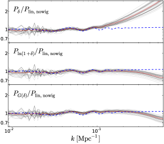
Figure 1.— Nonlinear transfer functions of 37 Coyote Universe simulations spanning a space of five cosmological parameters. The denominators in each panel are no-wiggle linear power spectra, without considering effects from the NGP pixel window function. The pixel window function causes the small-scale downturns in the bottom two panels (and attenuates $P_{\delta}$ as well). The dashed blue curves show the ratio of $P_{\rm lin}$ to $P_{\rm nowig}$. The dotted red curves are averages from the 37 simulations.

Fig. 1 shows, for each of 37 high-resolution simulations in the Coyote Universe (Heitmann et al., 2010, 2009; Lawrence et al., 2010) suite, ratios of $P_{\delta}$, $P_{\ln(1+\delta)}$ and $P_{G(\delta)}$ (the power spectrum of the rank-order-Gaussianized field $G(\delta)$, here mapping $\delta$ onto a Gaussian of unit variance), to the no-wiggle linear power spectrum $P_{\rm nowig}$ (Eisenstein & Hu, 1998), using that simulation’s cosmology.

Each curve is, essentially, a nonlinear transfer function, for a slightly different cosmology. There are important subtleties, though.

First, the power spectra are not divided by the power spectrum of the actual initial conditions, but the ensemble-average linear power spectrum (and a no-wiggle version of it, at that). Thus, cosmic-variance noise is present. However, we dampen this noise, by showing, for each density field, the average of the power spectra after applying 52 (up to the first harmonic in each direction) sinusoidal weightings (Hamilton et al., 2006, HRS).

Second, only the simulation power spectra (the numerator, but not the denominator) are attenuated by nearest-grid-point (NGP) pixel window functions. We plot each curve to its Nyquist wavenumber, where the attenuation is substantial. We did not correct for the pixel window function in the measurements because for $P_{\ln(1+\delta)}$ and $P_{G(\delta)}$, changing the resolution does more than simply introduce a small-scale attenuation, for example changing the large-scale amplitude. $P_{\ln(1+\delta)}$ and $P_{G(\delta)}$ do lack the nonlinear upward ramp at $k\gtrsim 0.1$ Mpc^-1 present in $P_{\delta}$, but starting at $k\approx 0.3$ Mpc^-1, they turn down compared to $P_{\rm nowig}$. Compare this to Fig. 3 of Paper I, in which the denominator is the power spectrum of the simulation’s exact initial conditions, including NGP attenuation (possible because of the much higher mass resolution in the Millennium simulation). In Fig. 3 of Paper I, the ratios do not depart substantially from unity. Thus we mainly ascribe the downturns in Fig. 1 to the resolution-dependent NGP pixel window function. The $P_{\delta}$ curves would also be higher than plotted at high $k$ without the NGP attenuation.

Finally, $P_{\ln(1+\delta)}$ and $P_{G(\delta)}$, generally biased on large scales compared to $P_{\delta}$, are multiplied by a factor to line up with $P_{\delta}$ in the smallest-$k$ bin shown. For $P_{G(\delta)}$, this process is equivalent to setting the variance of the Gaussian onto which $\delta$ is mapped so that the large-scale amplitude of $P_{G(\delta)}$ is the same as for $P_{\delta}$. In all further analysis below, for simplicity, we use a Gaussian with variance 1.

We rank-order-Gaussianize $\delta$ before the HRS weightings are applied, rather than Gaussianizing each weighted density field separately. Arguably, it would be fairest to Gaussianize each seperately, since the 1-point PDF of each weighted density field will slightly fluctuate from the PDF of the unweighted field. In real observations, one would be confronted with this fluctuated PDF, not the PDF from a larger sample. The main reason we Gaussianize before weighting is that practicically, it is nontrivial to Gaussianize the weighted density field, which has essentially a highly nonuniform (sinusoidal) selection function. Our procedure likely slightly overestimates the covariance from Gaussianizing the weighted density fields seperately, since this would equalize the variances in each. This would likely have similar covariance-killing effects as we found dividing $P_{\delta}$ by the density variance to have (Neyrinck, 2011).

Each simulation, analyzed at redshift $z=0$, has a different set of cosmological parameters, each a plausible (given current observational constraints) concordance cosmological model. The simulations occupy an orthogonal-array-Latin-hypercube in the five-dimensional parameter space $\omega_{m}=\Omega_{m}h^{2}\in[0.12,0.155]$, $\omega_{b}=\Omega_{b}h^{2}\in[0.0215,0.0235]$, $n_{s}\in[0.85,1.05]$, $w\in[-1.3,-0.7]$, $\sigma_{8}\in[0.61,0.9]$. The remaining cosmological parameters, e.g. $h$, are set to match the tight CMB constraint on the ratio of the last-scattering-surface distance to the sound-horizon scale. The 1024³-particle simulations have box size 1300 Mpc, fixed in Mpc (not  $h^{-1}$ Mpc) to roughly line up baryon-acoustic-oscillation (BAO) features in $k$ among different cosmologies. Their resolution is sufficient for power-spectrum measurements accurate at sub-percent level at scales down to $k=1$ $h$ Mpc^-1.

All the results in this paper use $256^{3}$ grids, a resolution at which shot noise is negligible even for $P_{\ln(1+\delta)}$ and $P_{G(\delta)}$. We do not push to smaller scales because even at this resolution, 25 of the simulations have handfuls of cells with zero particles. Among these 25, the median number of zero-particle cells is 19, with maximum 341, still $\ll 256^{3}$. To apply the log transform, we set the effective number of particles $N_{\rm eff}(N=0)=1/2$ in zero-particle cells, i.e. as though there were half a particle in the cell. This equalizes the distance in log-density between cells with 0 and 1 particle, and 1 and 2 particles. We experimented with changing $N_{\rm eff}(N=0)$ by factors of two up and down (to 1/4 and 1). Unsurprisingly, this had little effect; in the worst-case simulation with 341 zero-particle cells, $P_{\ln(1+\delta)}$ changed by at most (over all $k$) 0.03%, with typical changes $\sim$0.01%.

The level of fluctuation in the nonlinear transfer function looks substantially greater for $P_{\delta}$ than for $P_{\ln(1+\delta)}$ and $P_{G(\delta)}$ at large $k$, but around 0.1 Mpc^-1, there is not much difference. Some of the small-scale fluctuation could be from slight cosmology-dependent inaccuracies in the no-wiggle transfer function. Note that the dashed curve, showing the ratio of $P_{\rm lin}$, from camb (Lewis et al., 2000), to $P_{\rm nowig}$, departs slightly from 1 at large $k$.

By eye, the BAO are of similar amplitude in $P_{\ln(1+\delta)}$ and $P_{G(\delta)}$ as in $P_{\delta}$. This is not surprising; Gaussianizing does not undo the bulk motions that erase small-scale BAO wiggles in $P_{\delta}$. One difference, though, is that in $P_{\delta}$, the smallest-scale wiggles sit atop the start of the nonlinear ramp, which suggests that their detection may have to compete with a shot-noise-like (on translinear scales) one-halo term. Variance in this term can be seen as the source of the translinear covariance (Neyrinck et al., 2006). Note that in all panels, the BAO are likely a bit damped or smeared from the averaging over sinusoidal weightings, but to a lesser degree than the results below, which use up to the second harmonic in weightings. This dampening should affect all panels equally, and the scales of the weightings (just beyond the left edge of the plot) are $\sim 5$ times larger than BAO scales, so these effects are probably small. However, we leave a thorough quantitative analysis of BAO detection in Gaussianized power spectra to future work.

2.1. Covariance Matrices

We estimate the cumulative Fisher information (Fisher, 1935; Tegmark et al., 1997; Neyrinck & Szapudi, 2007) in parameters $\alpha$ and $\beta$ over a range of bin indices $i\in\mathcal{R}$ as

$$F_{\alpha\beta}(\mathcal{R})=\sum_{i,j\in\mathcal{R}}\frac{\partial\ln P_{i}}{\partial\alpha}(\textbf{{C}}_{\mathcal{R}}^{-1})_{ij}\frac{\partial\ln P_{j}}{\partial\beta},$$ (1)

where $\textbf{{C}}_{\mathcal{R}}$ is the square submatrix of the power-spectrum covariance matrix C with both indices ranging over $\mathcal{R}$. $C_{ij}\equiv\left\langle{\Delta\ln P_{i}\Delta\ln P_{j}}\right\rangle=\left\langle{\Delta P_{i}\Delta P_{j}}\right\rangle/\left\langle{P_{i}}\right\rangle\left\langle{P_{j}}\right\rangle$. The inverse of $F_{\alpha\beta}$ then gives the parameter covariance matrix.

In the bin range $\mathcal{R}$, $k_{\rm min}$ is the lowest $k$ not directly modulated by the sinusoidal weightings (beyond $\sqrt{3}$ times the wavenumber of the second harmonic), i.e. $k_{\rm min}=2\pi/(1300~{}{\rm Mpc})\times 2\sqrt{3}=0.017~{}{\rm Mpc}^{-1}$. We investigate constraints on parameters as $k_{\rm max}$ varies, up to the Nyquist frequency, $\sim 0.6~{}{\rm Mpc}^{-1}$. The bins of $k_{\rm max}$ vary by factors of $\sqrt[16]{2}$ (approximately, since each bin’s $k_{\rm max}$ is the mean $k_{\rm max}$ in the bin).

The power-spectrum covariance matrices are measured from the Coyote Universe suite, as in Neyrinck (2011). We used the HRS sinusoidal-weightings method, going up to the second harmonic to get 248 different power spectra from each simulation. This gave an estimate of the covariance in $\ln P$ from each simulation. We then formed an average covariance matrix across the simulations, to reduce noise. We averaged the covariances of $\ln P$ instead of $P$ for numerical stability across cosmologies; e.g. in linear theory, the covariance in $\ln P$ does not depend on the power spectrum.

Although using up to second-order weightings and then averaging together the covariance estimates among simulations beats down the noise in the covariance matrix substantially, the noise persists at a level that likely somewhat biases our results. This is because noise in a matrix that is inverted generally biases the inverse (Hartlap et al., 2007). Ideally, we would correct for the noise as suggested in that paper, but a necessary ingredient, the number of independent samples used for the covariance estimate, is not a straightforward quantity in the HRS weightings method. Each simulation gives 248 power spectra of overlapping subsamples; especially at low wavenumber, these power spectra are not necessarily independent. But this abundance of perhaps-redundant power spectra has the advantage of reducing the noise to a level low enough that e.g. it always provided naively invertible covariance matrices.

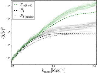
Figure 2.— The biasing effect of noise in the covariance matrix on the Fisher signal-to-noise ratio (S/N)². The faint curves show (S/N)², for both $P_{\delta}$ (black) and $P_{\ln(1+\delta)}$ (green), for each of the 37 simulations. The bold dashed curves show (S/N)², using the average covariance matrix used for the results below. (S/N)² for $P_{\delta}$ in the absence of noise may be estimated using the noise-free (but approximate) model of Neyrinck (2011) (dotted black). The proximity of the dashed and dotted black curves suggests a low level of residual bias in (S/N)² after averaging.

Fig. 2 illustrates the effect of noise on the signal-to-noise (S/N)², indicative of the (inverse) effect on parameter constraints, as well. Roughly, (S/N)² gives the number of statistically independent modes in the box, $\propto k_{\rm max}^{3}$ for a Gaussian field. It is measured by setting the derivative factors to unity in Eq. (1). The faint curves show (S/N)²  from each simulation; the bold dashed curves show (S/N)² using the averaged covariance, which we use for the results below (proportional to $1/\sqrt{(S/N)^{2}}$). Note that the scatter in the faint curves is not just from ordinary cosmic variance, but (predominantly) from the scatter in cosmological parameters among the simulations.

Fig. 2 shows that much bias in the Fisher matrix is eliminated by going from a single simulation to an average over 37. To assess the level of residual bias in (S/N)² after the averaging, we also show an estimate of the (S/N)² for $P_{\delta}$ using a noise-free approximate covariance matrix. We use the model of Neyrinck (2011), in which the covariance on translinear scales comes from scale-independent multiplicative fluctuations. Its only ingredient is the pixel-density variance, measurable with negligible noise. We averaged together the model covariance matrices in the same way as the full, measured ones. Comparing (S/N)² for $P_{\delta}$ to this model suggests that the residual bias is small. Importantly, the bias is also likely at the same level for all four power spectra investigated, so it probably does not affect our conclusions. Still, we keep in mind that our parameter constraints in all cases are likely slightly optimistic.

Fig. 3 shows the joint correlation matrix, $C_{ij}/\sqrt{C_{ii}C_{jj}}$, for both ($P_{\delta}(k)$, $P_{\ln(1+\delta)}(k)$) and ($P_{\delta}(k)$, $P_{G(\delta)}(k)$). We need their cross-covariance matrices below when we analyze pairs of power spectra together.

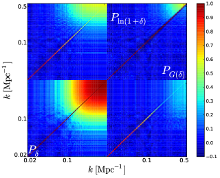
Figure 3.— Joint correlation matrices of ($P_{\delta}(k)$ and $P_{\ln(1+\delta)}(k)$), and ($P_{\delta}(k)$ and $P_{G(\delta)}(k)$). The lower-left square is the correlation matrix of $P_{\delta}$ alone. The upper-right square is the the correlation matrix of $P_{\ln(1+\delta)}$ alone (upper-left corner) and $P_{G(\delta)}$ alone (lower-right corner). The upper-left square is the cross-correlation between bins of $P_{\delta}$ and $P_{\ln(1+\delta)}$; the lower-right square is the same for $P_{\delta}$ and $P_{G(\delta)}$. The cross-correlation diagonals appear in Fig. 4.

Fig. 4 shows the cross-correlation diagonals, i.e. the correlations between $P_{\delta}(k)$ and $P_{\ln(1+\delta)}(k)$, and $P_{\delta}(k)$ and $P_{G(\delta)}(k)$, in the same $k$ bins. These cross-correlations are related to the nonlinear propagators (Crocce & Scoccimarro, 2006) of each power spectrum, since the nonlinear propagator of $P_{\delta}$ is unity on linear scales. The nonlinear propagator quantifies the memory of the particular Fourier phases and amplitudes of the initial conditions, as a function of $k$. For $P_{G(\delta)}$, this function dips down to $\sim 0.2$ on translinear scales.

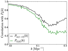
Figure 4.— Cross-correlations, measured at the same $k$ bin, between $P_{\delta}(k)$ and $P_{\ln(1+\delta)}(k)$, and $P_{\delta}(k)$ and $P_{G(\delta)}(k)$. These diagonals do dominate their respective cross-correlation matrices at low $k$. At high $k$ though, the curves become small, and are increasingly difficult to find amid the off-diagonal covariance.

The way we interpret this figure is that all three power spectra have similar nonlinear propagators, consistent with the findings of Wang et al. (2011). However, they each have different mode-coupling, or, roughly speaking, “one-halo” terms, correlated to each other only at the $\sim$20% level.

2.2. Derivative Terms

Here we describe how we estimate the derivative terms relevant for Fisher analysis, i.e. the vector $D_{i}(k)\equiv\partial\ln P(k)/\partial\alpha_{i}$. The Coyote Universe simulations were set up to span the 5-parameter space in an optimal way. Lawrence et al. (2010) employed sophisticated techniques such as principal-component analysis and Gaussian-process modeling to produce a precision power-spectrum emulator, CosmicEmu. They also used many lower-resolution simulations to analyze larger-scale modes, that we cannot use here because the Gaussianized power spectra are more sensitive to particle discreteness.

Our simpler approach is cruder, but acceptable for our purposes. In each $k$ bin, we model the fluctuations away from the mean power spectrum of all simulations as a linear combination of contributions from each parameter fluctuation, i.e.

$$\ln P^{\mbox{\boldmath$\alpha$}}(k)=\left\langle{\ln P(k)}\right\rangle+\mbox{\boldmath$D$}(k)\mbox{\boldmath$\cdot$}(\mbox{\boldmath$\alpha$}-\mbox{\boldmath$\bar{\alpha}$}),$$ (2)

where $\alpha$ is a vector in the space of the five parameters ($\ln\omega_{m}$, $\ln\omega_{b}$, $n_{s}$, $w$, $\ln\sigma_{8}^{2}$). $\bar{\alpha}$ is the mean of $\alpha$ over all simulations. Linear algebra yields an estimate of the derivative terms $\mbox{\boldmath$D$}(k)$ from a quintet of only five simulations, but it is unusably noisy, the signal swamped by cosmic variance in each simulation.

We enhance the signal in two ways. First, in each simulation, we use not the raw $P(k)$, but the ensemble-average of the power spectra of the density field after applying the 248 sinusoidal HRS weightings. This particularly squashes fluctuations away from the mean at small $k$, while preserving the overall shape. However, the window functions of the weightings likely convolve neighboring $k$ modes together somewhat. In particular, this probably dampens BAO wiggles a bit for all power spectra.

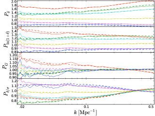
Figure 5.— Power spectra from Coyote Universe simulations 1-6 (solid), together with the predictions from Eq. (2). Cosmic-variance noise in each case has been dampened substantially by averaging over 248 HRS sinusoidal weightings. Only the fluctuation, second term on the RHS of Eq. (2) is shown, i.e. the geometric mean among the simulations is divided out.

Second, we estimate $\mbox{\boldmath$D$}(k)$ by finding the median in each $k$ bin among many estimates of $\mbox{\boldmath$D$}(k)$, each measured from a quintet sampled from the 37 simulations. Although the results visually converge with only $\sim 10^{3}$ quintets, we use $\sim 3\times 10^{6}$ quintets (limited by memory), looping through all quartets of simulations twice, each time choosing a random simulation to complete the quintet.

Fig. 5 shows power spectra from simulations 1-6, compared with their estimates from Eq. (2). Each power spectrum is divided by its geometric mean among the 37 simulations. Typically, the accuracy is at the few-percent level, with occasional deviations up to 10%. However, these larger deviations could be from cosmic variance in the particular simulation. We provide an emulator of these four power spectra, but caution prospective users to note the above caveats.

Fig. 6 shows $\mbox{\boldmath$D$}(k)$ estimated in this way for $P_{\rm lin}$ (estimated using camb), $P_{\delta}$, $P_{\ln(1+\delta)}$, $P_{G(\delta)}$, and $P_{\delta/\sigma}$ (the power spectrum of $\delta/\sigma_{\rm cell}$, the $\delta$ divided by its dispersion in cells). Except for $P_{\rm lin}$, and particularly in the latter three cases, these curves depend on the resolution used (a 256³ grid here). However, the general trends here should hold for different resolutions. For $P_{\delta}$, generally the results match those measured from the CosmicEmu emulator well. However, there is a large amount of noise that produces a discrepancy at small $k$ for $D_{\ln\omega_{b}}(k)$. This is by far the parameter with the smallest range explored; thus, it is not surprising that our rather crude method, without further low-resolution simulations for low-$k$ modes, is not quite adequate to explore it. For just the parameter $\omega_{b}$, we use $D_{\ln\omega_{b}}(k)$ evaluated from CosmicEmu for $P_{\delta}$. To all other power spectra, we add the correction $D_{\ln\omega_{b}}^{\mbox{\scriptsize{CosmicEmu}}}(k)-D_{\ln\omega_{b}}(k)$. This seems to improve the accuracy (or at least decrease the noise), but we caution that our results for $\omega_{b}$ are less accurate than for other parameters.

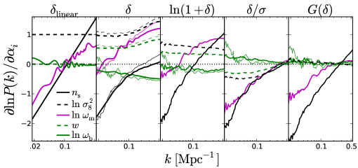
Figure 6.— Derivative terms $D_{i}(k)=\partial\ln P(k)/\partial\alpha_{i}$, quantifying the sensitivity of each power spectrum to the five explored cosmological parameters. The left panel is computed from camb. The second, $\delta$ panel shows $D_{i}(k)$ estimated as described in the text (thin), and from CosmicEmu (bold). For $\delta$, we use our own estimates of $D_{i}(k)$ for further calculations (except for $D_{\ln\omega_{b}}$, for which we use the CosmicEmu estimate). The (bold) curves in the rightmost three panels show our estimates of $D_{i}(k)$, that we use for further results. For $\omega_{b}$, a correction of $D_{\ln\omega_{b}}^{\mbox{\tiny{CosmicEmu}}}(k)-D_{\ln\omega_{b}}(k)$, measured for $P_{\delta}$, has been applied. The original $\omega_{b}$ measurements, without the correction, appear as the thin curves. Note that slight differences between curves are unlikely to be statistically significant, given the occasionally visible level of noise.

A few aspects of Fig. 6 should be pointed out. The parameter with the most straightforward connection to the power-spectrum shape is $n_{s}$, the tilt. The shape of $D_{n_{s}}(k)$ for $P_{\ln(1+\delta)}$ and $P_{G(\delta)}$ is nearly as straight as that for the linear power spectrum. In contrast, for $P_{\delta}$ and $P_{\delta/\sigma}$, $D_{n_{s}}(k)$ bends much more substantially at the onset of nonlinearity, indicating decreased sensitivity on small scales. This supports the claim that Gaussianization and the log-transform dramatically reduce nonlinearities in the power-spectrum shape.

A parameter whose simplicity is obscured by unfortunate notation is $\ln\sigma_{8}^{2}$, which we investigate instead of $\sigma_{8}$ because for all $\sigma_{8}$, $D_{\ln\sigma_{8}^{2}}(k)=1$ in linear theory. Reassuringly, like CosmicEmu, for this derivative we obtain about 1 on linear scales for $P_{\delta}$, as does CosmicEmu. At this cell resolution for $P_{\ln(1+\delta)}$, this derivative term is decreased to about 0.7, indicating decreased sensitivity of the mean power spectrum at each wavenumber. It is smaller than for $P_{\delta}$ because the log transform generally decreases the large-scale amplitude, by a factor of about $\exp(\sigma_{\rm cell}^{2})$ (Paper I).

In Fig. 6, all $P_{G(\delta)}$ and $P_{\delta/\sigma}$ derivative terms are tied together at zero at small scales. This is because for each, the variance is unity in $1300/256$ Mpc $\approx$ 4 $h^{-1}$ Mpc cells. The derivative terms are generally smaller in absolute value for these power spectra, which translates into poorer parameter constraints below than for $P_{\delta}$ and $P_{\ln(1+\delta)}$, with the exception of the parameter $n_{s}$. Curiously, at this resolution, $D_{\ln\sigma_{8}^{2}}(k)$ is of comparable absolute magnitude for $P_{\delta/\sigma}$ and $P_{\ln(1+\delta)}$ for small $k$. Naively, one might expect all information about the amplitude to be destroyed in $P_{\delta/\sigma}$, in which one divides the power spectrum by the variance in grid-cell densities (here, of 4 $h^{-1}$ Mpc size, but this holds to some degree for 8 $h^{-1}$ Mpc cells). However, recall that the amplitude $\sigma_{8}^{2}$ is the variance in 8 $h^{-1}$ Mpc volumes in the linearly, not nonlinearly, evolved density field; the nonzero $D_{\ln\sigma_{8}^{2}}(k)$ at small scales is apparently from the rise in the nonlinear power spectrum in $P_{\delta}$ and $P_{\delta/\sigma}$.

2.3. Error ellipses

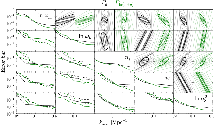
Figure 7.— Error-bar widths and error ellipses for $P_{\delta}$ (black) and $P_{\ln(1+\delta)}$ (green), in the Coyote-Universe space of five cosmological parameters. Along the diagonal, the curves are unmarginalized (half-)error bars over single parameters, holding all else fixed. Below the diagonal, pairs of parameters are considered; errors are shown in each parameter, marginalizing over the other. Solid curves correspond to the parameter of a panel’s row; dashed curves correspond to the column. Above the diagonal, error ellipses contract as $k_{\rm max}$ increases. The ellipses, in square panels of side half-length 0.5, are centered at the means of their parameters. An ellipse is drawn for each bin of $k_{\rm max}$ running from 0.02 to 0.6 Mpc^-1, log-spaced by a factor of $\sqrt[4]{2}$ (four times sparser than the bins constituting the curves). The bold ellipses are at $k_{\rm max}=0.1$. Outside, analyzing only large scales, $P_{\delta}$ and $P_{\ln(1+\delta)}$ both give similar constraints. Inside the bold ellipses, nonlinear scales, where $P_{\ln(1+\delta)}$ excels, are included, up to the innermost ellipse with $k_{\rm max}\approx 0.6$ Mpc^-1.

Fig. 7 shows error bars over the set of five cosmological parameters, for $P_{\delta}$ and $P_{\ln(1+\delta)}$. The effective volume for these results is (1.3 Gpc)${}^{3}/2\approx 1.1$ Gpc${}^{3}\approx.5$ ($h^{-1}$ Gpc)³. The factor of two is from the sinusoidal weightings used for the covariance matrices, which effectively halve the volume. Along the diagonal, the curves are unmarginalized error bars over single parameters, holding all else fixed. Off the diagonal, we examine error bars allowing sets of two parameters to vary at a time. The upper plots show how error ellipses contract as $k_{\rm max}$ increases, while the lower plots show how marginalized error bars shrink.

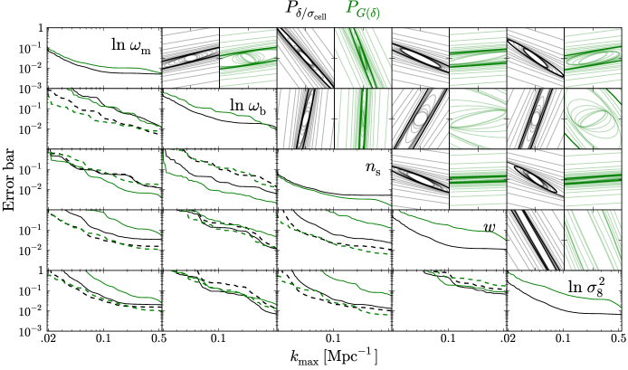
Figure 8.— Same as Fig. 7, for $P_{\delta/\sigma}$ and $P_{G(\delta)}$.

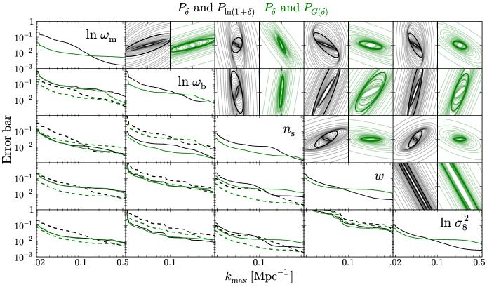
Figure 9.— Same as Fig. 7, except we show the constraints from analyzing both $P_{\delta}$ and $P_{\ln(1+\delta)}$, and $P_{\delta}$ and $P_{G(\delta)}$, together. For the combination of $P_{\delta}$ and $P_{\ln(1+\delta)}$, the constraints are about the minimum of the constraints from each power spectrum separately. For the $P_{\delta}$-$P_{G(\delta)}$ combination, though, there is some improvement when analyzing both together.

Constraints obtained analyzing $P_{\ln(1+\delta)}$ are substantially smaller than for $P_{\delta}$, for all parameters, typically by a factor of 2 or 3 if the analysis is pushed to the smallest scales shown. The difference is particularly large for $n_{s}$, where the error bar is reduced by a factor of 5. Another parameter whose behavior is simple to understand is $\ln\sigma_{8}^{2}$. As discussed above, $D_{\ln\sigma_{8}^{2}}(k)$ is smaller for $P_{\ln(1+\delta)}$ than for $P_{\delta}$, at all $k$. Looking at the diagonal, unmarginalized plots, this is why the error bars are degraded in $P_{\ln(1+\delta)}$ when only linear scales are included. However, when pushing into translinear scales, the penalty from the decreased derivative term is quickly overcome because of drastically reduced cosmic variance, resulting in tighter constraints from $P_{\ln(1+\delta)}$ at sufficiently small scales.

Fig. 8 shows the same figure for $P_{\delta/\sigma}$ and $P_{G(\delta)}$. Except for the case of the tilt $n_{s}$, the constraints from $P_{G(\delta)}$ are weaker than from $P_{\ln(1+\delta)}$, and often even weaker than from $P_{\delta}$. This could be surprising given that the covariance matrix of $P_{G(\delta)}$ has the smallest non-Gaussian component, and the highest diagonality, of any of the power spectra considered here. The performance of $P_{\delta/\sigma}$ is also disappointing given the high diagonality of its covariance matrix; the performance is also degraded for $P_{\delta/\sigma}$ compared to $P_{\delta}$ for some parameters. For $P_{G(\delta)}$ and $P_{\delta/\sigma}$, this behavior is from small derivative terms $\mbox{\boldmath$D$}(k)$. As discussed above, this is largely from the unit variance enforced in cell densities for these density fields.

Other analysis procedures are certainly possible. It would be convenient to use $P_{\delta}$ on linear scales, but on translinear scales, to exploit the reduced nonlinearity in the shape and covariance of $P_{G(\delta)}$. In principle, this could be done by setting the variance of the Gaussian in $P_{G(\delta)}$ so that the large-scale amplitude of $P_{G(\delta)}$ matches that of $P_{\delta}$, or equivalently multiplying $P_{G(\delta)}$ by a factor to line it up with $P_{\delta}$ on linear scales. We experimented with this, estimating this factor by averaging $P_{\delta}$$(k)/$$P_{G(\delta)}$$(k)$ over a range of $k$, but the uncertainty in this factor produced strong covariance on small scales, comparable to that of $P_{\delta}$. In fact, these experiments partially motivated the form of the $P_{\delta}$ covariance matrix found in Neyrinck (2011).

Fig. 9 shows the results from another possibility, in which we analyze $P_{\delta}$ and $P_{\ln(1+\delta)}$ together, and $P_{\delta}$ and $P_{G(\delta)}$ together. Generally, the constraints from analyzing two power spectra together are simply the minimum at each $k_{\rm max}$ of the results from analyzing each individually. This is unsurprising given the high, but not total, degeneracy between the power spectra. However, for the combination of $P_{\delta}$ and $P_{G(\delta)}$, there are significant gains over analyzing each individually for some parameter combinations, but the constraints are never better than for $P_{\ln(1+\delta)}$.

3. Discussion

We have explored the sensitivity to cosmological parameters of the power spectra of various transformations of the overdensity field. $P_{\delta}$, the conventional power spectrum, benefits from being exactly the linear power spectrum on linear scales. Another benefit of $P_{\delta}$ is in the simple effects of smoothing on it. However, on translinear scales it suffers strong nonlinearities, both in the mean shape and in the covariance, degrading parameter constraints.

$P_{\ln(1+\delta)}$, the power spectrum of the log-density, has the most cosmology-constraining power of any power spectrum considered here. Typically, pushing to the smallest scales analyzed here, constraints in marginalized and unmarginalized error bars are a factor of 2-3 smaller than for $P_{\delta}$. The generality of this result suggests that it would hold for other cosmological parameters as well. This improvement over $P_{\delta}$ comes from the high diagonality of $P_{\ln(1+\delta)}$’s covariance matrix, and from the small departures from the shape of the linear power spectrum. In particular, the tilt $n_{s}$ in the linear power spectrum is dramatically better-preserved in $P_{\ln(1+\delta)}$ than in $P_{\delta}$, as shown in its derivative terms in Fig. 6. The log transform reduces marginalized and unmarginalized error bars in $n_{s}$ by about a factor of 5.

$P_{G(\delta)}$, the power spectrum of the rank-order-Gaussianized density field, has a covariance matrix even more diagonal than $P_{\ln(1+\delta)}$, and exceeds $P_{\ln(1+\delta)}$ in cumulative signal-to-noise. Also, it can be directly applied in the case of significant discreteness noise (Neyrinck et al., 2011). This is unlike $P_{\ln(1+\delta)}$, although simple modifications of the log transform are possible to handle the problem. Unfortunately for cosmological constraints, though, Gaussianization as implemented here enforces a unit variance in cell densities. This degrades parameter constraints, in some cases to levels even worse than for $P_{\delta}$. A notable exception is $n_{s}$, for which constraints similar to $P_{\ln(1+\delta)}$ are obtained.

A promising approach explored by Joachimi et al. (2011) employs a Box-Cox transformation, which is a generalization of the logarithmic transform that can be calibrated to give a distribution with vanishing skewness and kurtosis. Perhaps this approach can reduce the non-Gaussian covariance to a level similar to the Gaussianization transform, while retaining some information about the power spectrum (e.g. its amplitude) on linear scales, as in the logarithmic transform.

$P_{\delta/\sigma}$, the power spectrum of the ratio $\delta/\sigma_{\rm cell}$, where $\sigma_{\rm cell}$ is $\delta$’s dispersion in few-Mpc cells, is the final power spectrum that we investigate. $P_{\delta/\sigma}$ has an impressively low non-Gaussian covariance, nearly to the level of $P_{G(\delta)}$. However, in a similar way as for $P_{G(\delta)}$, dividing by the dispersion erases much of the sensitivity to cosmological parameters, providing error bars similar to $P_{\delta}$.

4. Conclusion

We find that applying a nonlinear transform to the nonlinear density field can significantly enhance the cosmology-constraining power of the power spectrum, but apparently only if the transform preserves some linear-scale amplitude information. The log transform, for example, reduces error bars by a factor of 2-3; for the tilt, this factor reaches up to 5. The dramatic reduction in nonlinearities in both the power spectrum covariance (as quantified previously by the cumulative signal-to-noise ratio), and in the power spectrum shape, is what accomplishes this.

In Paper II, we showed that issues from galaxy discreteness, perhaps the most obvious problem for a logarithmic transform, can be overcome. A modified logarithmic transform still enhances the cumulative signal-to-noise ratio in the presence of discreteness noise. If the galaxy sampling is sufficiently dense, the tightening in parameter constraints found in the current paper will hold when applied to observations.

However, more work is required to investigate the cosmology sensitivity of power spectra of Gaussianized power spectra in the face of redshift-space distortions and galaxy bias. In Paper II, we began this study, but more work is required. Generally, fingers of God, present in redshift space, smear the density field, reducing the non-Gaussianity of the 1-point PDF, and thus somewhat decreasing the gains produced by a Gaussianizing transform.

Another important issue is whether Gaussianizing transforms are of use in detecting BAO. BAO scales are only barely translinear (transtranslinear?), even at $z=0$, so we expect the gains from covariance reduction alone to be modest. As we show qualitatively in Fig. 1, Gaussianizing transforms do not seem to alter the BAO wiggles substantially, with high-order wiggles erased similarly as in $P_{\delta}$ by large-scale bulk flows. However, the smallest-scale wiggle or two that are not washed out lie in the regime where the shot-noise-like one-halo term is significant, i.e. on the upward ramp in the nonlinear transfer function for $P_{\delta}$. This suggests that detecting the smallest-scale wiggles may be easier for $P_{\ln(1+\delta)}$ and $P_{G(\delta)}$.

As one might expect, there are some situations in which a log transform could be only marginally useful, and some in which it helps substantially. We are not aware of a case in which the transform degrades constraints, if the analysis is pushed to sufficiently small scales. But even if there is such a case, analyzing the conventional $P_{\delta}$ together with $P_{\ln(1+\delta)}$ or would give tighter constraints (if only marginally) than $P_{\delta}$ alone. Given the simplicity of these transforms, it seems to be well-worth using them observationally. This is even in cases that we have not directly tested, such as the highly nonlinear scales of the galaxy power spectrum or correlation function, sensitive to galaxy-formation details. In this case, one could also try looking at the ratio $P_{\delta}$/$P_{\ln(1+\delta)}$ (or even the ratio of the corresponding correlation functions).

References

- Box & Cox (1964) Box, G. E. P., & Cox, D. R. 1964, Journal of the Royal Statistical Society. Series B (Methodological), 26, pp. 211
- Carron (2011) Carron, J. 2011, ApJ, 738, 86, 1105.4467
- Coles & Jones (1991) Coles, P., & Jones, B. 1991, MNRAS, 248, 1
- Crocce & Scoccimarro (2006) Crocce, M., & Scoccimarro, R. 2006, Phys. Rev. D, 73, 063520, arXiv:astro-ph/0509419
- Eisenstein & Hu (1998) Eisenstein, D. J., & Hu, W. 1998, ApJ, 496, 605, arXiv:astro-ph/9709112
- Fisher (1935) Fisher, R. A. 1935, J. Roy. Stat. Soc., 98, 39
- Hamilton (2000) Hamilton, A. J. S. 2000, MNRAS, 312, 257, arXiv:astro-ph/9905191
- Hamilton et al. (2006) Hamilton, A. J. S., Rimes, C. D., & Scoccimarro, R. 2006, MNRAS, 371, 1188, arXiv:astro-ph/0511416
- Hartlap et al. (2007) Hartlap, J., Simon, P., & Schneider, P. 2007, A&A, 464, 399, arXiv:astro-ph/0608064
- Heitmann et al. (2009) Heitmann, K., Higdon, D., White, M., Habib, S., Williams, B. J., Lawrence, E., & Wagner, C. 2009, ApJ, 705, 156, 0902.0429
- Heitmann et al. (2010) Heitmann, K., White, M., Wagner, C., Habib, S., & Higdon, D. 2010, ApJ, 715, 104, 0812.1052
- Joachimi et al. (2011) Joachimi, B., Taylor, A. N., & Kiessling, A. 2011, MNRAS, 1390, 1104.1399
- Lawrence et al. (2010) Lawrence, E., Heitmann, K., White, M., Higdon, D., Wagner, C., Habib, S., & Williams, B. 2010, ApJ, 713, 1322, 0912.4490
- Lee & Pen (2008) Lee, J., & Pen, U.-L. 2008, ApJ, 686, L1, arXiv:0807.1538
- Lewis et al. (2000) Lewis, A., Challinor, A., & Lasenby, A. 2000, ApJ, 538, 473, arXiv:astro-ph/9911177, http://www.camb.info/
- Meiksin & White (1999) Meiksin, A., & White, M. 1999, MNRAS, 308, 1179, arXiv:astro-ph/9812129
- Neyrinck (2011) Neyrinck, M. C. 2011, ApJ, 736, 8, 1103.5476
- Neyrinck & Szapudi (2007) Neyrinck, M. C., & Szapudi, I. 2007, MNRAS, 375, L51, arXiv:astro-ph/0610211
- Neyrinck et al. (2006) Neyrinck, M. C., Szapudi, I., & Rimes, C. D. 2006, MNRAS, 370, L66, arXiv:astro-ph/0604282
- Neyrinck et al. (2009) Neyrinck, M. C., Szapudi, I., & Szalay, A. S. 2009, ApJ, 698, L90, 0903.4693 (Paper I)
- Neyrinck et al. (2011) ——. 2011, ApJ, 731, 116, 1009.5680 (Paper II)
- Rimes & Hamilton (2005) Rimes, C. D., & Hamilton, A. J. S. 2005, MNRAS, 360, L82, arXiv:astro-ph/0502081
- Rimes & Hamilton (2006) ——. 2006, MNRAS, 371, 1205, arXiv:astro-ph/0511418
- Romeo et al. (2008) Romeo, A. B., Agertz, O., Moore, B., & Stadel, J. 2008, ApJ, 686, 1, 0804.0294
- Scherrer et al. (2010) Scherrer, R. J., Berlind, A. A., Mao, Q., & McBride, C. K. 2010, ApJ, 708, L9, 0909.5187
- Scoccimarro et al. (1999) Scoccimarro, R., Zaldarriaga, M., & Hui, L. 1999, ApJ, 527, 1, arXiv:astro-ph/9901099
- Seo et al. (2011) Seo, H., Sato, M., Dodelson, S., Jain, B., & Takada, M. 2011, ApJ, 729, L11, 1008.0349
- Springel et al. (2005) Springel, V. et al. 2005, Nature, 435, 629, arXiv:astro-ph/0504097
- Szapudi & Kaiser (2003) Szapudi, I., & Kaiser, N. 2003, ApJ, 583, L1, arXiv:astro-ph/0211065
- Takahashi et al. (2009) Takahashi, R. et al. 2009, ApJ, 700, 479, 0902.0371
- Tegmark et al. (1997) Tegmark, M., Taylor, A. N., & Heavens, A. F. 1997, ApJ, 480, 22, arXiv:astro-ph/9603021
- Wang et al. (2011) Wang, X., Neyrinck, M., Szapudi, I., Szalay, A., Chen, X., Lesgourgues, J., Riotto, A., & Sloth, M. 2011, ApJ, 735, 32, 1103.2166
- Weinberg (1992) Weinberg, D. H. 1992, MNRAS, 254, 315
- Yu et al. (2011) Yu, Y., Zhang, P., Lin, W., Cui, W., & Fry, J. N. 2011, Phys. Rev. D, 84, 023523, 1103.2858
- Zhang et al. (2011) Zhang, T., Yu, H., Harnois-Déraps, J., MacDonald, I., & Pen, U. 2011, ApJ, 728, 35, 1008.3506