An Athermal Brittle to Ductile Transition in Amorphous Solids

Abstract

Brittle materials exhibit sharp dynamical fractures when meeting Griffith’s criterion, whereas ductile materials blunt a sharp crack by plastic responses. Upon continuous pulling ductile materials exhibit a necking instability which is dominated by a plastic flow. Usually one discusses the brittle to ductile transition as a function of increasing temperature. We introduce an athermal brittle to ductile transition as a function of the cut-off length of the inter-particle potential. On the basis of extensive numerical simulations of the response to pulling the material boundaries at a constant speed we offer an explanation of the onset of ductility via the increase in the density of plastic modes as a function of the potential cutoff length. Finally we can resolve an old riddle: in experiments brittle materials can be strained under grip boundary conditions, and exhibit a dynamic crack when cut with a sufficiently long initial slot. Mysteriously, in molecular dynamics simulations it appeared that cracks refused to propagate dynamically under grip boundary conditions, and continuous pulling was necessary to achieve fracture. We argue that this mystery is removed when one understands the distinction between brittle and ductile athermal amorphous materials.

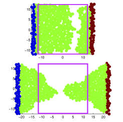
Figure 1: Color online: The result of pulling quasi-statically the side boundaries (the particles in the side walls are held frozen). Upper panel: the material is “brittle” and the pulling results in a clean crack. Lower panel: the material is “ductile” and the pulling induces a plastic flow with a necking instability. Note the large difference in the relative increase in system length compared to the original system size in the two panels. The number of particles $N=800$

I Introduction

Consider the following numerical experiment, which is also exhibited in Fig. 1 and in the movies available in movies . A piece of amorphous solid at rest is contained in the square (pink) box as plotted. The material is prepared by quenching a binary liquid of point particles (see potentials below), and removing the periodic boundaries. The resulting system has side walls consisting of pinned particles (identical to the bulk particles, blue and brown in Fig. 1) forming a rigid body which is pulled, the upper and lower boundaries are free. The walls are moved by an increment equal in size and opposite in sign.

In the upper panel the material is brittle, and cannot deform much before it fractures. In the lower panel the material is ductile, and the distance between the walls increases by about a factor of two before the plastic deformation that is induced creates a thin neck that is eventually broken. The huge difference in response is obtained with materials in the two panels that are identical in every respect except for the cutoff length of the attractive part of their inter-particle potentials, see Fig. 2. The aim of this paper is to explore the intrinsic relation between the microscopic properties of the inter-particle potential and the brittle to ductile transition. We explicitly do not consider in this paper the interesting effects of temperature, aspect ratio, system size and dimensionality, which of course are also important in determining a material’s brittleness.

One of our main motivations in this paper is a mystery that had clouded the fracture literature for a number of years now. The issue is crack propagation in amorphous solids under grip boundary conditions. In experiments one can pull the boundaries of a given sample and grip them, and then cut a slot at the edge of the sample 98HM . In brittle materials this leads to a fast development of the a dynamic fracture (when the length of the initial slot exceeds the Griffith’s length 98Fre ). For some unknown reason one always failed to repeat such experiments in direct molecular dynamic simulations, leading recently to some claims that only by defining ‘bonds’ between particles and letting these bonds ‘break’ under some criteria one can sustain a dynamical brittle fracture 11HKL . Obviously this is not a satisfactory answer; here we argue that the mystery is removed when one understands what makes a material brittle or ductile, and in truly brittle materials there is no problem in seeing a dynamical fracture under grip boundary conditions.

In this paper we want to understand how the response of an amorphous system subjected to uniaxial load depends on the parameters of the potential, and in particular the cut-off length $r_{\rm co}$. This will provide us with a fair insight into the athermal brittle to ductile transition. We will relate the degree of ductility to the growing importance of the contribution of ”plastic modes” to the density of states of the material.

The structure of this paper is as follows: In Sect. II we describe the glassy system used and how we control the range of the inter-particle potential. The numerical experiments and their results are described in Sect. III. In Sect. IV we relate and explain the findings of Sect. III to the density of states of the glassy materials, explaining that with increasing the range of the potential one changes the weight of the contribution of the plastic modes in the density of states. This correlates very well with the tendency towards ductility as seen in the numerical experiments. Finally in Sect.V we focus on the riddle of brittle fractures and show that there is no riddle at all - one simply needs to make the material brittle enough to allow brittle fractures to run spontaneously under grip boundary conditions. In Sect. VI we conclude the paper and reiterate the dramatic effect of the inter-particle’s potential properties on the behavior of a material under load 11KLPZ .

II System and Methods

For the numerical experiments we employ a generic glass former in 2-dimensions in the form of a binary mixture whose amount of bi-dispersity of ‘small’ and ‘large’ particles was chosen to avoid any crystallization. In fact the particles interact by inter-particle potentials as shown in Fig. 2, with the analytic form

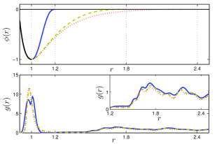
Figure 2: Color online: Upper panel: Examples of three different potentials with $r_{\rm co}=1.2,1.8$ and 2.4 used in our numerical experiments. The first and the third correspond to the experiment described in Fig. 1. Lower panel: the pair radial distribution function $g(r)$ for the three corresponding potentials in the upper panel. Note that the second shell of neighbors begins around $r=1.5$

$$\phi\!\left(\!{\textstyle\frac{r_{ij}}{\lambda_{ij}}}\!\right)=\left\{\begin{array}[]{ccl}&&4\varepsilon\left[\left(\frac{\lambda_{ij}}{r_{ij}}\right)^{12}-\left(\frac{\lambda_{ij}}{r_{ij}}\right)^{6}\right]\ ,\hskip 99.58464pt\frac{r_{ij}}{\lambda_{ij}}\leq\frac{r_{\rm min}}{\lambda}\\ &&\varepsilon\left[a\left(\frac{\lambda_{ij}}{r_{ij}}\right)^{12}-b\left(\frac{\lambda_{ij}}{r_{ij}}\right)^{6}+\displaystyle{\sum_{\ell=0}^{3}}c_{2\ell}\left({\textstyle\frac{r_{ij}}{\lambda_{ij}}}\right)^{2\ell}\right]\ ,\hskip 14.22636pt\frac{r_{\rm min}}{\lambda}<\frac{r_{ij}}{\lambda_{ij}}<\frac{r_{\rm co}}{\lambda}\\ &&\quad\quad\quad\quad 0\ ,\hskip 153.6447pt\frac{r_{ij}}{\lambda_{ij}}\geq\frac{r_{\rm co}}{\lambda}\end{array}\right.\!\!$$ (1)

Here $r_{\rm min}/\lambda_{ij}$ is the length where the potential attain it’s minimum, and $r_{\rm co}/\lambda_{ij}$ is the cut-off length for which the potential vanishes. The coefficients $a,~{}b$ and $c_{2\ell}$ are chosen such that the repulsive and attractive parts of the potential are continuous with two derivatives at the potential minimum and the potential goes to zero continuously at $r_{\rm co}/\lambda_{ij}$ with two continuous derivatives as well. The interaction length-scale $\lambda_{ij}$ between any two particles $i$ and $j$ is $\lambda_{ij}=1.0\lambda$, $\lambda_{ij}=1.18\lambda$ and $\lambda_{ij}=1.4\lambda$ for two ‘small’ particles, one ‘large’ and one ‘small’ particle and two ‘large’ particle respectively. The unit of length $\lambda$ is set to be the interaction length scale of two small particles, $\varepsilon$ is the unit of energy and $k_{B}=1$.

The systems employed in the pulling experiments consist of configurations which were quenched from systems initially equilibrated at high temperature and pressure ($T=1.0,\ P=1.0$) with periodic boundary conditions. The number of particles $N$ varied between $N=800$ and $N=67000$. We used a modified Berendsen thermostat which couples a constant number of particles to the bath, regardless of the system size 10KLPZ . The systems are cooled to temperature $T=10^{-2}$ while keeping the pressure high, in order to avoid the creation of any holes in the material. Then the pressure is reduced to zero, $P=0.0$, such that the periodic boundary conditions could be removed; particles forming the right and left walls were frozen, but the upper and lower boundaries were rendered free.

From this point the system was treated differently for the brittle crack and the necking experiments. The brittle crack experiment starts by loading the system uniaxially (with a constant velocity such that $v_{\rm wall}\ll c_{s}/10$) until a desired stress is reached, and then the side walls are held fixed. A cut is then implemented by the cancelation of forces crossing an imaginary line of desired length which starts at the lower boundary. The evolution of the crack is simulated by molecular dynamics at $T=0.0$ and requires no further loading of the system.

The necking experiments were conducted in athermal quasi-static conditions. For those experiments the systems were further minimized with respect to the acting forces on each particle, making them athermal. The right and left walls were then moved with a strain increment $\delta\ell=5\cdot 10^{-3}$. The response we investigate is the relative increase in the system’s length $\Gamma=\Delta L/L$ along the stretching direction. The maximal value that the system is able to accommodate before it breaks into two parts is denoted as $\Gamma_{\rm max}$ footnote .

III Numerical Experiments and Results

In this paper we describe only 2-dimensional simulations with a square initial geometry. In fact we have set up samples of height $H$ and length $L=aH$, with $a\in[1,5]$, but we did not find any exciting aspect-ratio dependence beyond the obvious. For the square initial geometry the athermal response was characterized by $\Gamma_{\rm max}$. In Fig. 3 we exhibit the dependence of $\Gamma_{\rm max}$ on $r_{\rm co}$ for square systems $(a=1)$.

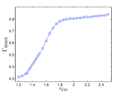
Figure 3: Color online: The dependence of $\Gamma_{\rm max}$ on $r_{\rm co}$ for the geometry of Fig. 1 (square initial conditions). Note that $\Gamma_{\rm max}$ tends to saturate at a given value $\Gamma^{\infty}_{\rm max}$ which becomes independent on $r_{\rm co}$; in athermal conditions it depends on the geometry of the sample only.

It is sufficient to limit the range of the potential cut-off to

$$r_{\rm co}\in[1.2\lambda;\ 2.5\lambda].$$ (2)

The lower limit for $r_{\rm co}$ is dictated by the position of the first peak in $g(r)$ cf. Fig. 2 lower panel. For $r_{\rm co}<1.2$ the potential gets shorter than the first shell of neighbors. The upper limit is determined by the convergence of our 1-parameter family of potentials to the asymptotic Lennard-Jones potential. Within this range of potentials $\langle\Gamma_{\rm max}\rangle$ was evaluated by averaging over 4500 samples. It is found to increase smoothly with $r_{\rm co}$ reaching a limiting value $\Gamma^{\infty}_{\rm max}$. When the system reaches the limiting value $\Gamma^{\infty}_{\rm max}$ we refer to it as “maximally ductile”.

The qualitative understanding of the result shown in Fig. 3 is quite straightforward. In the limit $r_{\rm co}\to r_{\rm min}$ any cavity that forms whose dimensions is larger than $r_{\rm co}$ will not heal since there are no attractive forces operating across it. Rather, it will propagate rapidly to span the system in a form of a brittle fracture. With $r_{\rm co}$ increasing, a small cavity will still be held by attractive forces across it. The higher is $r_{\rm co}$ the larger is the number of neighbors that each particles feels attracted to, and one needs to create a very large cavity indeed to overcome these attractive forces. On the other hand when $r_{\rm co}$ increases beyond the second shell of the binary correlation function, not much can change. With our choice of potentials, in the limit $r_{\rm co}\to\infty$ we simply converge to the infinite-range Lennard-Jones potential which has a negligible attractive force beyond, say, $r/\lambda=3$. This qualitative understanding is further supported by examining the contribution of the plastic modes to the density of states, as we do next.

IV The contribution of plastic modes

It is well known that in amorphous solids the density of states deviates from the classical Debye formula which was developed for a perfect elastic solid. The deviations were referred to as the ’Boson peak’ but very little reliable analytic statements were made about the form of this deviation 09IPRS . In recent work of the present group it was proposed that one can provide a useful analytic form of the density of states (the HKLP model 11HKLP ) which will be particularly useful at the low end tail of frequencies. In terms of the eigenvalues of the Hessian matrix $\lambda_{i}=\omega^{2}_{i}$ where $\omega_{i}$ is the $i$’th normal mode frequency the proposed model is

$$P\left(\frac{\lambda}{\lambda_{D}}\right)=Nd\left[\frac{d}{2}\left(\frac{\lambda}{\lambda_{D}}\right)^{(d-2)/2}+B\left(\frac{\lambda}{\lambda_{D}}\right)^{\theta}\right]\ ,$$ (3)

where the first term on the RHS is the Debye formula in which $N$ is the number of particles, $d$ the space dimension and $\lambda_{D}$ is the Debye cutoff frequency which in 2-dimensions reads $\lambda_{D}=8\pi\mu$ with $\mu$ being the shear modulus. The second term is our proposed addition to the model density of states that should be appropriate for all generic amorphous solids in the limit $\lambda\ll\lambda_{D}$. This term contains contributions from eigenvalues $\lambda_{i}$ that depend on the external mechanical loading, and go to zero with increasing the load, harking the appearance of plastic instabilities 11HKLP . The exponent $\theta$ in this plastic contribution is not universal, it depends on the amount of disorder in the glassy system, and it was shown to be an important characteristic of the mechanical properties of amorphous solids 11HKLP .

In numerical calculations it is easier to evaluate the cumulative distribution $C(\lambda)\equiv\int_{0}^{\lambda}P(\tilde{\lambda})d\tilde{\lambda}$, whose form is

$$C\left(\frac{\lambda}{\lambda_{D}}\right)=Nd\left[\left(\frac{\lambda}{\lambda_{D}}\right)^{d/2}+\frac{B}{1+\theta}\left(\frac{\lambda}{\lambda_{D}}\right)^{1+\theta}\right]\ .$$ (4)

In the present context we wish to understand the relation between the tendency towards ductility as $r_{\rm co}$ increases to the amount of plasticity as expressed, say, by the value of the weight coefficient $B$ and the exponent $\theta$. To this aim we have computed the cumulative density of states $C\left(\frac{\lambda}{\lambda_{D}}\right)$ and subtracted from it the exactly known Debye contribution. The resulting plots are shown in Fig. 4. We see that the model 3 is faithfully representing the data for small values of $r_{\rm co}$, whereas for the largest ones the amount of plastic modes increases beyond the first term contribution in the model. This is however not causing any difficulty in estimating the weight $B$ (the intercept in Fig. 4) which is shown in Fig. 5.

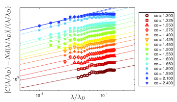
Figure 4: Color online: the cumulative density of states from which the Debye contribution was subtracted. The remaining plastic contribution is plotted in log-log coordinates such that the intercept is $B/(1+\theta)$ and the slope is $\theta$.

It is quite obvious that our $\Gamma_{\rm max}$ dependence on $r_{\rm co}$ (cf. Fig. 3) is qualitatively similar to the dependence of the weight $B$ on $r_{\rm co}$. It is therefore natural to plot $\Gamma_{\rm max}$ as a function of $B$. A convincing linear dependence can be obtained by plotting $\Gamma_{\rm max}$ as a function of $B^{2}$ as is shown in Fig. 5.

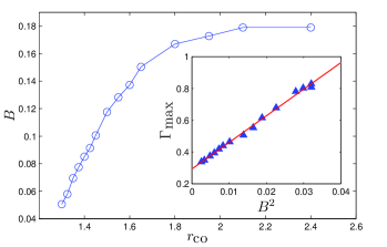
Figure 5: Color online: the value of the weight $B$ in Eq. 4 as a function of $r_{\rm co}$. Inset: $\Gamma_{\rm max}$ vs. $B^{2}$.

V The brittle crack

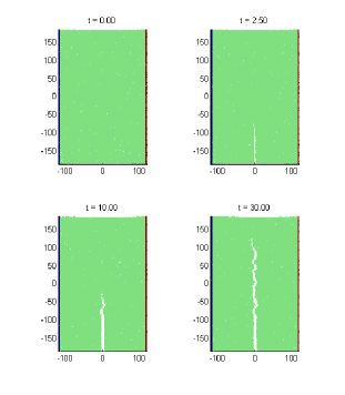
Figure 6: Color online: the development of a brittle crack under grip boundary conditions. The finite size effect appears as bending of the upper boundary, releasing the stress before the fracture hits the boundary.

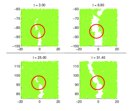
Figure 7: Color online: the development of a brittle crack appears many times to consist of the creation of a cavity ahead of the crack, followed by a necking process in which the cavity and the body of the crack coalesce. Shown are two such events, where the left panels exhibit the cavities ahead of the crack, and the right panels exhibit the crack after the necking events coalesced the crack with the cavities.

We are now able to construct a system where all the microscopic parameters are tuned to minimize the occurrence of plastic events, a system which can be denoted ‘maximally brittle’. We expect such a system to fail under grip boundary conditions upon the application of a cut in one of the free boundaries. For a large value of $r_{\rm co}$, a small cavity can still be held by attractive forces across it. The longer is $r_{\rm co}$ the larger is the number of neighbors that each particles feels attracted to, and one needs to create a very large cavity indeed to overcome these attractive forces. On the other hand, in the limit of $r_{\rm co}\to r_{\rm min}$ any cavity that forms whose dimensions is larger than $r_{\rm co}$ cannot heal since there are no attractive forces operating across it. Rather, it would propagate rapidly to span the system in a form of a brittle fracture. The system we used to demonstrate this concept is composed of $N=67000$ particles with a cut-off length of $r_{\rm co}=1.20$ and $\varepsilon=10.0$; this choice was made to increase the stability of the system and prevents any unwanted events during the loading part of the simulation. The experiment is run by means of molecular dynamics at $T=0.0$. The size of the cut is 100$\lambda$. The evolution of the crack can be appreciated in Fig. 6.

When the fracture originates from a cut, the system does not need to create a cavity in order to propagate a crack. The stress field around the tip of the cut is greatly enhanced by the strong curvature of the boundary, and once the Griffith’s criterion is fulfilled the crack can run. Nevertheless during the propagation of the crack we observe many times the formation of a cavity ahead of the crack tip followed by necking to coalesce the cavity with the body of the crack. The observed dynamics is presented in Fig. 7, which employs snapshots from the brittle crack development that is shown in Fig. 6. We note in passing that this mechanism of propagation of brittle cracks was seen experimentally in Ref. 99BP . In Ref. 04BMP this same mechanism was proposed as the reason for the roughening of the fracture surface. This roughening is seen to the bare eye in Fig. 6; its quantitative assessment and its relation to the mechanism in question will be considered in a future publication.

VI summary and conclusions

The main result of this paper is the dramatic change in material mechanical properties that results from changing the inter-particle potential interaction length. We introduced the athermal brittle to ductile transition, showing that even at $T=0$ we can go all the way from brittle to ductile response only by changing the cutoff length $r_{\rm co}$. There is an interesting analogy between increasing the cutoff length and raising the temperature; in both case the system becomes ‘softer’. This softening can be quantitatively described by our model of density of states of amorphous solids, in which the coefficient $B$ measures the increasing weight of plastic modes, which are those eigenfunctions of the Hessian matrix whose eigenvalues vanish in saddle-node bifurcations when the system is strained 11HKLP . Indeed, we found a linear dependence between the degree of lengthening of the system before breaking and $B^{2}$. Finally, the new understanding of brittleness vs. ductility allowed us to disperse a long standing conundrum - how to get a brittle crack running under grip boundary conditions. It turns out that previous attempts failed simply because the system chosen were not brittle enough. Building a ‘maximally brittle’ material results in a nice running crack under grip boundary conditions as seen in many experiments.