Enhancing or suppressing spin Hall effect of light in layered nanostructures

Abstract

The spin Hall effect (SHE) of light in layered nanostructures is investigated theoretically in this paper. A general propagation model describing the spin-dependent transverse splitting of wave packet in the SHE of light is established from the viewpoint of classical electrodynamics. We show that the transverse displacement of wave-packet centroid can be tuned to either a negative or a positive value, or even zero, by just adjusting the structure parameters, suggesting that the SHE of light in layered nanostructures can be enhanced or suppressed in a desired way. The inherent physics behind this interesting phenomenon is found to be attributed to the optical Fabry-Perot resonance. We believe that these findings will open the possibility for developing new nano-photonic devices.

I Introduction

Spin Hall effect (SHE) is a transport phenomenon, in which an applied field on the spin particles leads to a spin-dependent displacement perpendicular to the electric field direction Murakami2003 ; Sinova2004 ; Wunderlich2005 . The SHE of light can be regarded as a direct optical analogy of SHE in electronic system where the spin electrons and electric potential are replaced by spin photons and refractive index gradient, respectively Onoda2004 ; Bliokh2006 ; Hosten2008 . The SHE of light is sometimes referred to as the Fedorov-Imbert effect, which was predicted theoretically by Fedorov Fedorov1965 , and experimentally confirmed by Imbert Imbert1972 . The spin-dependent transverse shift in the SHE of light is generally believed as a result of an effective spin-orbital interaction, which describes the mutual influence of the spin (polarization) and trajectory of the light beam Bliokh2007 .

Recently, the SHE of light has been extensively investigated in different physical systems. In a static gravitational field, the photon Hamiltonian shows a new kind of helicity-torsion coupling, resulting in a novel birefringence phenomenon: photons with distinct helicity follow different geodesics Gosselin2007 . In optical systems, the SHE of light is observed directly in the glass cylinder and its fundamental origin is related to the dynamical action of the topological Berry-phase monopole in the evolution of light Bliokh2008 . The SHE of light can also be observed in scattering from dielectric spheres Haefner2009 . In particular, a giant SHE of light can be produced by subwavelength displacements of a nanoparticle Herrera2010 . Even in free space, the SHE of light can be observed on the direction tilted with respect to beam propagation axis Aiello2009 . In plasmonic systems, a spin-dependent splitting of the focal spot of a plasmonic focusing lens was demonstrated and explained in terms of a geometric phase Gorodetski2008 . In semiconductor physics, the SHE of light has been observed in silicon via free-carrier absorption. The interesting result suggests that the SHE of light has the potential of probing spatial distributions of electron spin states Menard2010 .

The SHE may offer an effective way to manipulate the spin particles, and open a promising way to some potential applications, such as in dense data storage, ultra-fast information processing, and even quantum computing Wolf2001 ; Chappert2007 ; Awschalom2007 . The generation, manipulation, and detection of spin-polarized electrons in semiconductors and nanostructures define the main challenges of spin-based electronics. Similar challenges also exist in spin-based photonics. The SHE of light may open new opportunities for manipulating photon spin and developing new generation of all-optical devices as counterpart of recently presented spintronics devices. In this paper, we will study the SHE of light in layered nanostructures in which the refractive indices of their constituent materials vary between high-index regions and low-index regions. Such an environment presents to photons as an analogy of semiconductor presenting potential to electrons Joannopoulos1995 , thus presenting some imaginable interesting properties of the SHE of light.

The paper is organized as follows. First, we want to establish a three-dimensional propagation model to describe the SHE of light in layered nanostructure. The Fresnel coefficients are no longer real in the layered nanostructures, so it is necessary for us to obtain a more general expression. Next, we attempt to reveal what roles the Fresnel reflection and transmission coefficients play in the SHE of light. We find that the Fresnel coefficients present sine-like oscillations and the spin-dependent splitting of wave-packet centroid significantly depends on their ratio. Finally, we want to explore the secret underlying this interesting phenomenon. The result shows that the SHE of light can be readily modulated, i.e., enhanced or suppressed, via tuning the optical resonance in layered nanostructures.

II Three-dimensional beam propagation model

Figure 1 illustrates the beam reflection and refraction in the layered nanostructure. The $z$ axis of the laboratory Cartesian frame ($x,y,z$) is normal to the interfaces of the layered structure. We use the coordinate frames ($x_{a},y_{a},z_{a}$) for central wave vector, where $a=i,r,t$ denotes incident, reflection, and transmission, respectively. We apply the angular spectrum method to derive an expression for a three-dimensional beam propagation model. Hence, we use local Cartesian frames ($X_{a},Y_{a},Z_{a}$) to describe an arbitrary angular spectrum. The electric field of the $a$th beam can be solved by employing the Fourier transformations. The complex amplitude for the $a$th beam can be conveniently expressed as Goodman1996

$$\mathbf{E}_{a}(x_{a},y_{a},z_{a}) = \int dk_{ax}dk_{ay}\tilde{\mathbf{E}_{a}}(k_{ax},k_{ay})$$ (1)

$$\times\exp[i(k_{ax}x_{a}+k_{ay}y_{a}+k_{az}z_{a})],$$

where $k_{az}=\sqrt{k_{a}^{2}-(k_{ax}^{2}+k_{ay}^{2})}$ and $\tilde{\mathbf{E}_{a}}(k_{ax},k_{ay})$ is the angular spectrum. The approximate paraxial expression for the field in Eq. (1) can be obtained by the expansion of the square root of $k_{az}$ to the first order Lax1975 , which yields

$$\mathbf{E}_{a} = \exp(ik_{a}z_{a})\int dk_{ax}dk_{ay}\tilde{\mathbf{E}_{a}}(k_{ax},k_{ay})$$ (2)

$$\times\exp\left[i\left(k_{ax}x_{a}+k_{ay}y_{a}-\frac{k_{ax}^{2}+k_{ay}^{2}}{2k_{a}}z_{a}\right)\right].$$

In general, an arbitrary linear polarization can be decomposed into horizontal and vertical components. In the spin basis set, the angular spectrum can be written as:

$$\tilde{E}_{i}^{H}=\frac{1}{\sqrt{2}}(\tilde{\mathbf{E}}_{i+}+\tilde{\mathbf{E}}_{i-}),$$ (3)

$$\tilde{E}_{i}^{V}=\frac{1}{\sqrt{2}}i(\tilde{\mathbf{E}}_{i-}-\tilde{\mathbf{E}}_{i+}).$$ (4)

Here, $H$ and $V$ represent horizontal and vertical polarizations, respectively. The positive and negative signs denote the left and right circularly polarized (spin) components, respectively Beth1936 . The monochromatic Gaussian beam can be formulated as a localized wave packet whose spectrum is arbitrarily narrow, and can be written as

$$\tilde{\mathbf{E}}_{i\pm}=\frac{1}{\sqrt{2}}(\mathbf{e}_{ix}\pm i\mathbf{e}_{iy})\frac{w_{0}}{\sqrt{2\pi}}\exp\left[-\frac{w_{0}^{2}(k_{ix}^{2}+k_{iy}^{2})}{4}\right],$$ (5)

where $w_{0}$ is the beam waist. After the angular spectrum is known, we can obtain the field characteristics for the $a$th beam.

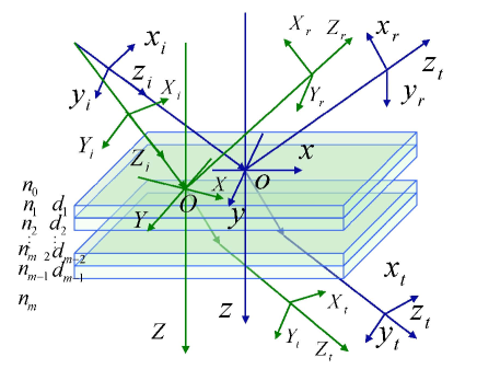
Figure 1: (color online) Schematic illustrating the reflection and refraction of central and local wave vectors at $(m+1)$-layered nanostructure. $x_{a}y_{a}z_{a}$ ($a=i,r,t$) are reference frames for central wave vector of incident, reflection, and transmission, respectively. $oxyz$ and $OXYZ$ are the interface reference frames for central and local wave vectors, respectively.

To accurately describe the SHE of light in layered nanostructure, it is need to determine the reflection and transmission of arbitrary wave-vector components, which can be solved by $2\times 2$ transmission matrix Yariv2007 :

$$\mathbb{M}=T_{01}P_{1}T_{12}P_{2}...P_{m-2}T_{m-2,m-1}P_{m-1}T_{m-1,m},$$ (6)

where

$$T_{m-1,m}=\frac{1}{t_{m-1,m}}\left[\begin{array}[]{cc}1&r_{m-1,m}\\ r_{m-1,m}&1\end{array}\right],$$ (9)

is the transformation matrix from $(m-1)$-th to $m$-th layer, and

$$P_{m}=\left[\begin{array}[]{cc}\exp(ik_{mz}d_{m})&0\\ 0&\exp(-ik_{mz}d_{m})\end{array}\right],$$ (12)

is the transmission matrix for $m$-th layer. Here, $d_{m}$ is the thickness of $m$-th layer, $r_{m-1,m}$ and $t_{m-1,m}$ are reflection and transmission coefficients from $(m-1)$-th to $m$-th layer, respectively. For an arbitrary wave-vector component, the Fresnel coefficients of the layered nanostructures can be written as

$$t_{p,s}=\frac{1}{\mathbb{M}_{11}},~{}~{}~{}~{}~{}r_{p,s}=\frac{\mathbb{M}_{21}}{\mathbb{M}_{11}},$$ (13)

where $p$ and $s$ denote parallel and perpendicular polarizations, respectively. By making use of Taylor series expansion, the Fresnel coefficients can be expanded as a polynomial of $k_{ix}$. We obtain a sufficiently good approximation when the Taylor series are confined to the zero order.

From the boundary condition, we obtain $k_{rx}=-k_{ix}$ and $k_{ry}=k_{iy}$. After a series of calculations of the reflected angular spectrum given in the Appendix A, Eq. (2) together with Eqs. (13) and (52) provides the paraxial expression of the reflected field:

$$\mathbf{E}_{r\pm}^{H} = \frac{r_{p}(\mathbf{e}_{rx}\pm i\mathbf{e}_{ry})}{\sqrt{\pi}w_{0}}\frac{z_{R}}{z_{R}+iz_{r}}\exp(ik_{r}z_{r})$$ (14)

$$\times\exp\left[-\frac{k_{0}}{2}\frac{x_{r}^{2}+(y_{r}\pm\delta_{r}^{H})^{2}}{z_{R}+iz_{r}}\right],$$

$$\mathbf{E}_{r\pm}^{V} = \frac{\mp ir_{s}(\mathbf{e}_{rx}\pm i\mathbf{e}_{ry})}{\sqrt{\pi}w_{0}}\frac{z_{R}}{z_{R}+iz_{r}}\exp(ik_{r}z_{r})$$ (15)

$$\times\exp\left[-\frac{k_{0}}{2}\frac{x_{r}^{2}+(y_{r}\pm\delta_{r}^{V})^{2}}{z_{R}+iz_{r}}\right],$$

where $z_{R}=k_{0}w_{0}^{2}/2$ is the Rayleigh lengths, $\delta_{r}^{H}=(1+r_{s}/r_{p})\cot\theta_{i}/k_{0}$ and $\delta_{r}^{V}=(1+r_{p}/r_{s})\cot\theta_{i}/k_{0}$.

We next consider the transmitted field. From the Snell’s law under the paraxial approximation, we obtain $k_{tx}=k_{ix}/\eta$ and $k_{ty}=k_{iy}$. Substituting Eqs. (13) and (65) into Eq. (2), we obtain the transmitted field:

$$\mathbf{E}_{t\pm}^{H} = \frac{t_{p}(\mathbf{e}_{tx}\pm i\mathbf{e}_{ty})}{\sqrt{\pi}w_{0}}\frac{z_{Ry}\exp(ik_{t}z_{t})}{\sqrt{(z_{Rx}+iz_{t})(z_{Ry}+iz_{t})}}$$ (16)

$$\times\exp\left[-\frac{n_{m}k_{0}}{2}\left(\frac{x_{t}^{2}}{z_{Rx}+iz_{t}}+\frac{(y_{t}\mp\delta_{t}^{H})^{2}}{z_{Ry}+iz_{t}}\right)\right],$$

$$\mathbf{E}_{t\pm}^{V} = \frac{\mp it_{s}(\mathbf{e}_{tx}\pm i\mathbf{e}_{ty})}{\sqrt{\pi}w_{0}}\frac{z_{Ry}\exp(ik_{t}z_{t})}{\sqrt{(z_{Rx}+iz_{t})(z_{Ry}+iz_{t})}}$$ (17)

$$\times\exp\left[-\frac{n_{m}k_{0}}{2}\left(\frac{x_{t}^{2}}{z_{Rx}+iz_{t}}+\frac{(y_{t}\mp\delta_{t}^{V})^{2}}{z_{Ry}+iz_{t}}\right)\right].$$

Here, $\delta_{t}^{H}=(\eta-t_{s}/t_{p})\cot\theta_{i}/k_{0}$ and $\delta_{t}^{V}=(\eta-t_{p}/t_{s})\cot\theta_{i}/k_{0}$. The interesting point we want to stress is that there are two different Rayleigh lengths, $z_{Rx}=n_{m}\eta^{2}k_{0}w_{0}^{2}/2$ and $z_{Ry}=n_{m}k_{0}w_{0}^{2}/2$, characterizing the spreading of the beam in the direction of $x$ and $y$ axes, respectively Luo2009 . Note that the Fresnel coefficients are no longer real in the layered nanostructure. Hence, we should extend the previous expression of transverse displacement Hosten2008 to a more general situation.

III Spin Hall effect of light

It is well known that the SHE of light manifests itself as polarization-dependent transverse splitting. To reveal the SHE of light, we now determine the transverse displacements of field centroid. The time-averaged linear momentum density associated with the electromagnetic field can be shown to be Jackson1999

$$\mathbf{p}_{a}(\mathbf{r})=\frac{1}{2c^{2}}\mathrm{Re}[\mathbf{E}_{a}(\mathbf{r})\times\mathbf{H}_{a}^{\ast}(\mathbf{r})],$$ (18)

where the magnetic field can be obtained by $\mathbf{H}_{a}=-ik_{a}^{-1}\nabla\times\mathbf{E}_{a}$. The intensity distribution of wave packet is closely linked to the longitudinal momentum currents $I(x_{a},y_{a},z_{a})\propto\mathbf{p}_{a}\cdot\mathbf{e}_{az}$.

At any given plane $z_{a}=\text{const.}$, the transverse displacement of wave-packet centroid compared to the geometrical-optics prediction is given by

$$\Delta y_{a}=\frac{\int\int y_{a}I(x_{a},y_{a},z_{a})\text{d}x_{a}\text{d}y_{a}}{\int\int I(x_{a},y_{a},z_{a})\text{d}x_{a}\text{d}y_{a}}.$$ (19)

Note that the transverse displacement can be divided into $z_{a}$-dependent and $z_{a}$-independent terms. We here concentrate our attention on the $z_{a}$-independent transverse displacements.

We first consider the spin-dependent transverse displacement of the reflected field. After substituting the reflected field Eqs. (14) and (15) into Eq. (19), we obtain the transverse spatial displacements as

$$\Delta y_{r\pm}^{H}=\mp\frac{\lambda}{2\pi}[1+|r_{s}|/|r_{p}|\cos(\varphi_{s}-\varphi_{p})]\cot\theta_{i},$$ (20)

$$\Delta y_{r\pm}^{V}=\mp\frac{\lambda}{2\pi}[1+|r_{p}|/|r_{s}|\cos(\varphi_{p}-\varphi_{s})]\cot\theta_{i},$$ (21)

where $r_{p,s}=|r_{p,s}|\exp(i\varphi_{p,s})$. Note that these expressions are slightly different from the previous work Hosten2008 ; Qin2009 , since the Fresnel reflection coefficients are no longer real in our model.

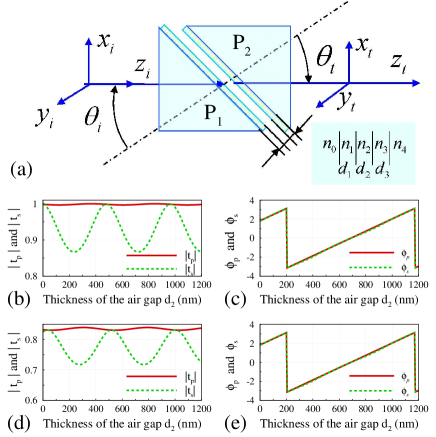
Figure 2: (Color online) The Fresnel transmission coefficients in a five-layered nanostructure. (a) Schematic illustrating the layered nanostructure: The two prisms (P₁ and P₂) both filmed by a low refractive index layer with $n_{1}=n_{3}=1.377$ ($\mathrm{MgF_{2}}$ at 633 nm), $d_{1}=d_{3}=80nm$, and the thickness of the air gap ($d_{2}$) can be modulated. The incident angle is chosen as $\theta_{i}=\pi/6$. The Fresnel transmission coefficients $t_{p}$ and $t_{s}$ versus the thickness of the air gap $d_{2}$ for the the symmetric and asymmetric system: (b) $n_{0}=n_{4}=1.515$ (BK7 at 633 nm) and (d) $n_{0}=1.515$ (BK7 at 633 nm) and $n_{4}=1.996$ (S-LAH79 at 633 nm). (c) and (e) are the phase of the Fresnel transmission coefficients for the two systems, respectively.

We next consider the spin-dependent transverse displacements of the transmitted field. After substituting the transmitted field Eqs. (16) and (17) into Eq. (19), we have

$$\Delta y_{t\pm}^{H}=\pm\frac{\lambda}{2\pi}[\eta-|t_{s}|/|t_{p}|\cos(\phi_{s}-\phi_{p})]\cot\theta_{i},$$ (22)

$$\Delta y_{t\pm}^{V}=\pm\frac{\lambda}{2\pi}[\eta-|t_{p}|/|t_{s}|\cos(\phi_{p}-\phi_{s})]\cot\theta_{i},$$ (23)

where $t_{p,s}=|t_{p,s}|\exp(i\phi_{p,s})$. For an arbitrary linearly polarized incident beam, the calculation of the transverse displacements for the reflected and transmitted field is given in the Appendix B.

For left and right circularly polarized components, the eigenvalues of the transverse displacement are the same in magnitude but opposite in directions. Under the limit of $m=1$ (air-glass interface), the above expression coincides well with the early results Bliokh2007 . Our scheme shows that the SHE of light can be explained from the viewpoint of classic electrodynamics. For incidence angles greater than the critical angle of total internal reflection, most of photons are reflected, and part of them tunnel through the layered structure Luo2010 . Hereafter, we only concentrate our attention on the SHE of light in the transmission case.

As an example, a five-layered nanostructure composed of two prisms (P₁ and P₂), two films ($\mathrm{MgF_{2}}$), and an air gap [Fig. 2(a)] is chosen to illustrate the SHE of light. We consider two kind of systems: (i) A symmetric system with two BK7 prisms ($n_{0}=n_{4}=1.515$ at 633 nm) filmed by $\mathrm{MgF_{2}}$ ($n_{1}=n_{3}=1.377$ at 633 nm) and the middle layer is air gap ($n_{2}=1$); (ii) Replacing P₂ by an S-LAH79 prism ($n_{4}=1.996$ at 633 nm) to form an asymmetric system. The $\mathrm{MgF_{2}}$ layers with 80 nm thickness were prepared on P₁ and P₂. For a given incident angle $\theta_{i}=\pi/6$, $t_{s}$ in the two systems both behave sine-like oscillations versus to the thickness of air gap ($d_{2}$) due to the optical Febry-Perot resonance with multi-resonant peaks for different $d_{2}$, while $t_{p}$ is nearly unchanged and insensitive to $d_{2}$ [Fig. 2(b) and 2(d)]. It is obvious that $|t_{s}|/|t_{p}|\cos(\phi_{s}-\phi_{p})$ and $|t_{p}|/|t_{s}|\cos(\phi_{p}-\phi_{s})$ in Eqs. (22) and (23) determine the magnitude of the transverse displacements ($\Delta y_{t\pm}$) of wave-packet centroid since other quantities in the two equations are constant. Actually, the $\phi_{p}$ is nearly equal to $\phi_{s}$ versus $d_{2}$ for both the symmetric [Fig. 2(c)] and asymmetric system [Fig. 2(e)], which means $\cos(\phi_{p}-\phi_{s})\approx 1$ and the magnitude of $\Delta y_{t\pm}$ only depends on $|t_{s}|/|t_{p}|$ or $|t_{p}|/|t_{s}|$.

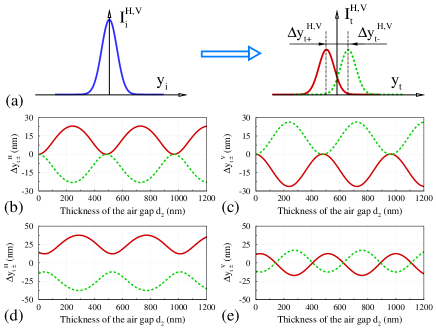
Figure 3: (Color online) (a) Schematic illustrating the spin-dependent transverse splitting. The transverse displacements versus the thickness of the air gap $d_{2}$ in the situation of transmission with incident angle $\theta_{i}=\pi/6$. (b) and (c) show the transverse displacements of $H$ and $V$ components, respectively, for the symmetric system. (d) and (e) also represent the transverse displacements but for the asymmetric system.

The spin-dependent splitting in SHE of light is schematically shown in Fig. 3(a). From Eqs. (22) and (23), we know that the transverse displacements of $H$ and $V$ polarizations would have just opposite tendency versus $d_{2}$ which can also be seen from Fig. 3(b)-3(e). For a fixed incident angle of $\theta_{i}=\pi/6$, the transverse displacements present sine-like oscillations since the value of $|t_{s}|/|t_{p}|$ or $|t_{p}|/|t_{s}|$ is periodic due to the Fabry-Perot resonance in the layered structures. In the symmetric case, the transverse displacements present a sine-like oscillation in the range of zero-positive-zero or zero-negative-zero for a certain polarization component [Fig. 3(b)-3(c)]. In the asymmetric case, for $H$-polarization, the transverse displacements can exhibit a positive and negative transverse displacement for left- and right-polarized components, respectively [Fig. 3(d)]. It is interesting to note that the transverse displacements exhibits a sine-like oscillation in the range of negative-zero-positive values for $V$-polarization, which can be modulated via tuning the thickness of the air gap [Fig. 3(e)]. It indicates that the SHE of light can be greatly enhanced or suppressed, or even completely eliminated.

From the above analysis, we know that the transverse displacements are related to the ratio between the Fresnel transmission coefficients $|t_{p}|$ and $|t_{s}|$, whose dependence on the thickness of the air gap are periodic due to the Fabry-Perot resonance in the layered nanostructures. Hence, we can expect that a nanostructure with a large ratio of $|t_{s}|/|t_{p}|$ or $|t_{p}|/|t_{s}|$ would extremely enhance the SHE of light. On the contrary, a small ratio of $|t_{s}|/|t_{p}|$ or $|t_{p}|/|t_{s}|$ would greatly suppress the SHE of light. In fact, the phase difference $\phi_{p}-\phi_{s}$ of the Fresnel transmission coefficients may also be used to modulate the SHE of light since it can change the sign of $\Delta y_{t\pm}$. The nanostructures with a metamaterial layer whose refractive index can be tailored arbitrarily can be a good candidate to support this prediction Luo2009 . Under the condition of $|t_{s}|/|t_{p}|\cos(\phi_{s}-\phi_{p})=\eta$ ($H$ polarization) and $|t_{p}|/|t_{s}|\cos(\phi_{p}-\phi_{s})=\eta$ ($V$ polarization), the SHE of light can be suppressed completely.

It should be mentioned that the spatial separation of the spin components can also be tuned continuously by varying the incident angle in a single air-glass interface Hosten2008 . However, the refracted angle changes and the transmission coefficients decrease accordingly as the incident angle increases. Hence, it is disadvantage for potential application to nano-photonic devices. As shown in above, the wave packet in our scheme is incident at a fixed angle, and the transverse displacements can be tuned to either a negative or a positive value, or even zero, by just adjusting the structure parameters. Meanwhile, the wave packet in the layered nanostructure exhibit much higher transmission coefficients than in the single air-glass interface. Hence, the layered nanostructures provide more flexibility for modulating the SHE of light. We will search for suitable nanostructures to manipulate it in the future. It is expected that the SHE of light in layered nanostructures will be useful for designing very fast optical switches, for example, by replacing the air gap by material whose refractive index can be tuned by a electric field.

IV Conclusions

In conclusion, we have revealed a tunable SHE of light in layered nanostructures. From the viewpoint of classical electrodynamics, we have established a general propagation model to describe the spin-dependent transverse splitting of wave packet in the SHE of light. By modulating the structure parameters, the transverse displacements exhibit tunable values ranging from negative to positive, including zero, which means that the SHE of light can be greatly enhanced or suppressed, or completely eliminated. We have shown that the physical mechanism underlying this intriguing phenomenon is the optical Fabry-Perot resonance in the layered nanostructure. These findings provide a pathway for modulating the SHE of light, and thereby open the possibility for developing new nano-photonic devices.

Appendix A Calculation of the reflected and transmitted angular spectra

In this appendix we give a detailed calculation of the reflected and transmitted angular spectra. From the central frame $x_{i}y_{i}z_{i}$ to the local frame $X_{i}Y_{i}Z_{i}$, the following three steps should be carried out. First, we transform the electric field from the reference frame $x_{i}y_{i}z_{i}$ around the $y$ axis by the incident angle $\theta_{i}$ to the frame $xyz$: $\tilde{E}_{xyz}=m_{{x_{i}y_{i}z_{i}}\rightarrow{xyz}}\tilde{E}_{x_{i}y_{i}z_{i}}$, where

$$m_{{x_{i}y_{i}z_{i}}\rightarrow{xyz}}=\left[\begin{array}[]{ccc}\cos\theta_{i}&0&-\sin\theta_{i}\\ 0&1&0\\ \sin\theta_{i}&0&\cos\theta_{i}\end{array}\right].$$ (27)

Then, we transform the electric field from the reference frame $xyz$ around the $y$ axis by an angle $k_{iy}/(k_{0}\sin\theta_{i})$ to the frame $XYZ$, and the correspondingly matrix is given by

$$m_{{xyz}\rightarrow{XYZ}}=\left[\begin{array}[]{ccc}1&\frac{k_{iy}}{k_{0}\sin\theta_{i}}&0\\ -\frac{k_{iy}}{k_{0}\sin\theta_{i}}&1&0\\ 0&0&1\end{array}\right],$$ (31)

where $k_{0}$ is the wave number in vacuum. Finally, we transform the electric field from the reference frame $XYZ$ around the $y$ axis by an angle $-\theta_{i}$ to the frame $X_{i}Y_{i}Z_{i}$, and the matrix can be written as

$$m_{{XYZ}\rightarrow{X_{i}Y_{i}Z_{i}}}=\left[\begin{array}[]{ccc}\cos\theta_{i}&0&\sin\theta_{i}\\ 0&1&0\\ -\sin\theta_{i}&0&\cos\theta_{i}\end{array}\right].$$ (35)

Thus, the rotation matrix from the central frame $x_{i}y_{i}z_{i}$ to the local frame $X_{i}Y_{i}Z_{i}$ can be written as $M_{{x_{i}y_{i}z_{i}}\rightarrow{X_{i}Y_{i}Z_{i}}}=m_{{XYZ}\rightarrow{X_{i}Y_{i}Z_{i}}}m_{{xyz}\rightarrow{XYZ}}m_{{x_{i}y_{i}z_{i}}\rightarrow{xyz}}$, and we have

$$M_{{x_{i}y_{i}z_{i}}\rightarrow{X_{i}Y_{i}Z_{i}}}=\left[\begin{array}[]{ccc}1&\frac{k_{iy}\cot\theta_{i}}{k_{0}}&0\\ -\frac{k_{iy}\cot\theta_{i}}{k_{0}}&1&\frac{k_{iy}}{k_{0}}\\ 0&-\frac{k_{iy}}{k_{0}}&1\end{array}\right].$$ (39)

For an arbitrary wave vector, the reflected field is determined by $\tilde{E}_{X_{r}Y_{r}Z_{r}}=r_{p,s}\tilde{E}_{X_{i}Y_{i}Z_{i}}$, where $r_{p}$ and $r_{s}$ are the Fresnel reflection coefficients. The reflected field should be transformed from $X_{r}Y_{r}Z_{r}$ to $x_{r}y_{r}z_{r}$. Following the similar procedure, the reflected field can be obtained by carrying out three steps of transformation: $\tilde{E}_{x_{r}y_{r}z_{r}}=M_{{X_{r}Y_{r}Z_{r}}\rightarrow{x_{r}y_{r}z_{r}}}\tilde{E}_{X_{r}Y_{r}Z_{r}}$ where

$$M_{{X_{r}Y_{r}Z_{r}}\rightarrow{x_{r}y_{r}z_{r}}}=\left[\begin{array}[]{cc}1&\frac{k_{ry}\cot\theta_{i}}{k_{0}}\\ -\frac{k_{ry}\cot\theta_{i}}{k_{0}}&1\end{array}\right].$$ (42)

Here, only the two-dimensional rotation matrices is taken into account, since the longitudinal component of electric field can be obtained from the divergence equation $\tilde{E}_{az}k_{az}=-(\tilde{E}_{ax}k_{ax}+\tilde{E}_{ay}k_{ay})$. The reflection matrix can be written as

$$M_{R}=M_{{X_{r}Y_{r}Z_{r}}\rightarrow{x_{r}y_{r}z_{r}}}\left[\begin{array}[]{cc}r_{p}&0\\ 0&r_{s}\end{array}\right]M_{{x_{i}y_{i}z_{i}}\rightarrow{X_{i}Y_{i}Z_{i}}}.$$ (45)

The reflected angular spectrum is related to the boundary distribution of the electric field by means of the relation $\tilde{E}_{r}(k_{rx},k_{ry})=M_{R}\tilde{E}_{i}(k_{ix},k_{iy})$, and we have

$$\left[\begin{array}[]{cc}\tilde{E}_{r}^{H}\\ \tilde{E}_{r}^{V}\end{array}\right]=\left[\begin{array}[]{cc}r_{p}&\frac{k_{ry}(r_{p}+r_{s})\cot\theta_{i}}{k_{0}}\\ -\frac{k_{ry}(r_{p}+r_{s})\cot\theta_{i}}{k_{0}}&r_{s}\end{array}\right]\left[\begin{array}[]{cc}\tilde{E}_{i}^{H}\\ \tilde{E}_{i}^{V}\end{array}\right],$$ (52)

We proceed to consider the transmitted field. Following the similar procedure, we obtain the transform matrix from $X_{t}Y_{t}Z_{t}$ to $x_{t}y_{t}z_{t}$ as

$$M_{{X_{t}Y_{t}Z_{t}}\rightarrow{x_{t}y_{t}z_{t}}}=\left[\begin{array}[]{cc}1&-\frac{k_{ty}\cos\theta_{t}}{k_{0}\sin\theta_{i}}\\ \frac{k_{ty}\cos\theta_{t}}{k_{0}\sin\theta_{i}}&1\end{array}\right],$$ (55)

where $\theta_{t}$ is the transmitted angle. For an arbitrary wave vector, the transmitted field is determined by $\tilde{E}_{X_{t}Y_{t}Z_{t}}=t_{p,s}\tilde{E}_{X_{i}Y_{i}Z_{i}}$, where $t_{p}$ and $t_{s}$ are the Fresnel transmission coefficients. Hence, the transmission matrix can be written as

$$M_{T}=M_{{X_{t}Y_{t}Z_{t}}\rightarrow{x_{t}y_{t}z_{t}}}\left[\begin{array}[]{cc}t_{p}&0\\ 0&t_{s}\end{array}\right]M_{{x_{i}y_{i}z_{i}}\rightarrow{X_{i}Y_{i}Z_{i}}}.$$ (58)

The transmitted angular spectrum is related to the boundary distribution of the electric field by means of the relation $\tilde{E}_{t}(k_{tx},k_{ty})=M_{T}\tilde{E}_{i}(k_{ix},k_{iy})$, and can be written as

$$\left[\begin{array}[]{cc}\tilde{E}_{t}^{H}\\ \tilde{E}_{t}^{V}\end{array}\right]=\left[\begin{array}[]{cc}t_{p}&\frac{k_{ty}(t_{p}-\eta t_{s})\cot\theta_{i}}{k_{0}}\\ \frac{k_{ty}(\eta t_{p}-t_{s})\cot\theta_{i}}{k_{0}}&t_{s}\end{array}\right]\left[\begin{array}[]{cc}\tilde{E}_{i}^{H}\\ \tilde{E}_{i}^{V}\end{array}\right],$$ (65)

where $\eta=\cos\theta_{t}/\cos\theta_{i}$.

Appendix B Transverse displacements for arbitrary linear polarization

For an arbitrary linearly polarized beam, the transverse displacements of the reflected field are given by

$$\Delta y_{r\pm}=\cos^{2}\gamma_{r}\Delta y_{r\pm}^{H}+\sin^{2}\gamma_{r}\Delta y_{r\pm}^{V},$$ (66)

where $\gamma_{r}$ is the reflected polarization angle. In the frame of classical electrodynamics, the reflection polarization angle is determined by:

$$\cos\gamma_{r}=\frac{\cos\gamma_{i}\mathrm{Re}[r_{p}]}{\sqrt{\cos^{2}\gamma_{i}\mathrm{Re}[r_{p}]^{2}+\sin^{2}\gamma_{i}\mathrm{Re}[r_{s}]^{2}}},$$ (67)

$$\sin\gamma_{r}=\frac{\sin\gamma_{i}\mathrm{Re}[r_{s}]}{\sqrt{\cos^{2}\gamma_{i}\mathrm{Re}[r_{p}]^{2}+\sin^{2}\gamma_{i}\mathrm{Re}[r_{s}]^{2}}}.$$ (68)

Here, $\gamma_{i}$ is the incident polarization angle. For an arbitrary linearly polarized wave-packet, the transverse displacements of the transmitted field are given by

$$\Delta y_{t\pm}=\cos^{2}\gamma_{t}\Delta y_{t\pm}^{H}+\sin^{2}\gamma_{t}\Delta y_{t\pm}^{V},$$ (69)

where the transmission polarization angle $\gamma_{t}$ determined by

$$\cos\gamma_{t}=\frac{\cos\gamma_{i}\mathrm{Re}[t_{p}]}{\sqrt{\cos^{2}\gamma_{i}\mathrm{Re}[t_{p}]^{2}+\sin^{2}\gamma_{i}\mathrm{Re}[t_{s}]^{2}}},$$ (70)

$$\sin\gamma_{t}=\frac{\sin\gamma_{i}\mathrm{Re}[t_{s}]}{\sqrt{\cos^{2}\gamma_{i}\mathrm{Re}[t_{p}]^{2}+\sin^{2}\gamma_{i}\mathrm{Re}[t_{s}]^{2}}}.$$ (71)

References

• (1) S. Murakami, N. Nagaosa, and S. C. Zhang, Science 301, 1348 (2003).
• (2) J. Sinova, D. Culcer, Q. Niu, N. A. Sinitsyn, T. Jungwirth, and A. H. MacDonald, Phys. Rev. Lett. 92, 126603 (2004).
• (3) J. Wunderlich, B. Kaestner, J. Sinova, and T. Jungwirth, Phys. Rev. Lett. 94, 047204 (2005).
• (4) M. Onoda, S. Murakami, and N. Nagaosa, Phys. Rev. Lett. 93, 083901 (2004).
• (5) K. Y. Bliokh and Y. P. Bliokh, Phys. Rev. Lett. 96, 073903 (2006).
• (6) O. Hosten and P. Kwiat, Science 319, 787 (2008).
• (7) F. I. Fedorov, Dokl. Akad. Nauk SSSR 105, 465 (1955).
• (8) C. Imbert, Phys. Rev. D 5, 787 (1972).
• (9) K. Y. Bliokh and Y. P. Bliokh, Phys. Rev. E 75, 066609 (2007).
• (10) P. Gosselin, A. Bérard, and H. Mohrbach, Phys. Rev. D 75, 084035 (2007).
• (11) K. Y. Bliokh, A. Niv, V. Kleiner, and E. Hasman, Nature Photon. 2, 748 (2008).
• (12) D. Haefner, S. Sukhov, and A. Dogariu, Phys. Rev. Lett. 102, 123903 (2009).
• (13) O. G. Rodríguez-Herrera, D. Lara, K. Y. Bliokh, E. A. Ostrovskaya, and C. Dainty, Phys. Rev. Lett. 104, 253601 (2010).
• (14) A. Aiello, N. Lindlein, C. Marquardt, and G. Leuchs, Phys. Rev. Lett. 103, 100401 (2009).
• (15) Y. Gorodetski, A. Niv, V. Kleiner, and E. Hasman, Phys. Rev. Lett. 101, 043903 (2008).
• (16) J.-M. Ménard, A. E. Mattacchione, H. M. van Driel, C. Hautmann, and M. Betz, Phys. Rev. B 82, 045303 (2010).
• (17) S. A. Wolf, D. D. Awschalom, R. A. Buhrman, J. M. Daughton, S. von Molnár, M. L. Roukes, A. Y. Chtchelkanova, and D. M. Treger, Science 294, 1488 (2001).
• (18) C. Chappert, A. Fert, and F. N. V. Dau, Nature 6, 813, (2007).
• (19) D. D. Awschalom and M. E. Flatte, Nature Phys. 3, 153 (2007).
• (20) J. D. Joannopoulos, R. D. Meade, and J. N. Winn, Photonic Crystals: Molding the Flow of Light (Princeton Univ. Press, Princeton, 1995).
• (21) J. W. Goodman, Introduction to Fourier Optics (McGraw-Hill, New York, 1996).
• (22) M. Lax, W. H. Louisell, and W. McKnight, Phys. Rev. A 11, 1365 (1975).
• (23) R. A. Beth, Phys. Rev. 50, 115 (1936).
• (24) A. Yariv and P. Yeh, Photonics: Optical Electronics in Modern Communications (Oxford University Press, New York, 2007).
• (25) H. Luo, S. Wen, W. Shu, Z. Tang, Y. Zou, and D. Fan, Phys. Rev. A 80, 043810 (2009).
• (26) J. D. Jackson, Classical Electrodynamics (Wiley, New York, 1999).
• (27) Y. Qin, Y. Li, H. Y. He, and Q. H. Gong, Opt. Lett. 34, 2551 (2009).
• (28) H. Luo, S. Wen, W. Shu, and D. Fan, Phys. Rev. A 82, 043825 (2010).