Probing the GC-LMXB connection in NGC 1399: a wide-field study with HST and Chandra .

Abstract

We present a wide field study of the Globular Clusters/Low Mass X-ray Binary (LMXB) connection in the giant elliptical NGC1399. The large FOV of the ACS/WFC, combined with the HST and Chandra high resolution, allow us to constrain the LMXB formation scenarios in elliptical galaxies. We confirm that NGC1399 has the highest LMXB fraction in GCs of all nearby elliptical galaxies studied so far, even though the exact value depends on galactocentric distance due to the interplay of a differential GC vs galaxy light distribution and the GC color dependence. In fact LMXBs are preferentially hosted by bright, red GCs out to $>5\,R_{\rm eff}$ of the galaxy light. The finding that GC hosting LMXBs follow the radial distribution of their parent GC population, argues against the hypothesis that the external dynamical influence of the galaxy affects LMXB formation in GCs. On the other hand field LMXBs closely match the host galaxy light, thus indicating that they are originally formed in situ and not inside GCs. We measure GC structural parameters, finding that the LMXB formation likelihood is influenced independently by mass, metallicity and GCs structural parameters. In particular the GC central density plays a major role in predicting which GC host accreting binaries. Finally our analysis shows that LMXBs in GCs are marginally brighter than those in the field, and in particular the only color-confirmed GC with $L_{X}>10^{39}$ erg s^-1 shows no variability, which may indicate a superposition of multiple LMXBs in these systems.

1. Introduction

A significant contribution from accreting binary stars to the total X-ray emission of early-type galaxies has been predicted for a long time, using the X-ray/optical luminosity ratio and spectral energy distribution (see Fabbiano, 1989, and references therein) as primary indicators, long before the majority of X-ray sources could be resolved individually. With the launch of Chandra, with its sub-arcsecond spatial resolution, tens to hundreds of low-mass X-ray binaries (LMXB) were discovered in nearby ellipticals, a large number of which are residing in Globular Clusters (GC), with a complex dependence on the properties of the host galaxy and of the GC population.

Several studies have shown that while on average a few percent ($\sim\!5\%$) of GCs host LMXBs, the fraction of LMXBs residing in GCs varies from $10\!-\!20\%$ in late-type galaxies and reaches up to $\sim\!70\%$ in cD galaxies, depending on the morphological type of the galaxy and on the GC specific frequency (see review in Fabbiano, 2006). It was also observed that LMXBs reside preferentially in bright GCs (Angelini et al., 2001; Kundu et al., 2002; Sarazin et al., 2003; Kim et al., 2006; Kundu et al., 2007; Sivakoff et al., 2007), as expected if dynamical interactions favor binary formation in dense environments (Clark, 1975; White et al., 2002; Pooley et al., 2003; Verbunt, 2005). More puzzling is the dependence of the probability of finding LMXBs on the GC color. Recent studies indicate that red (old, metal-rich) GCs are $\sim\!3$ times more likely to host LMXBs than blue (young, metal-poor) ones (Angelini et al., 2001; Kundu et al., 2002; Sarazin et al., 2003; Jordán et al., 2004; Kim et al., 2006; Kundu et al., 2007; Sivakoff et al., 2007).

The spatial distribution of LMXBs is also debated: while some studies find that the spatial distribution of GC-LMXBs is more extended than field-LMXBs (Kim et al., 2006; Kundu et al., 2007), others do not observe such a difference (e.g Humphrey & Buote, 2008). The issue is further complicated by the fact that for a proper comparison with the distribution of host GCs, the samples must be split according to GC colors (see Fabbiano, 2006, and references therein).

Constraining these observables is crucial for discriminating among LMXB formation models. For instance, irradiation-induced winds (Maccarone et al., 2004), magnetic breaking (Ivanova, 2006) or IMF variations (Grindlay, 1987, Jordán et al., 2004, also see) can explain the LMXB formation likelihood as a function of the host GC color in terms of a metallicity effect, while other dynamical models (e.g Kim et al., 2006; Jordán et al., 2007a; Sivakoff et al., 2007) suggest that this color dependence may reflect the higher LMXB formation efficiency in more centrally-concentrated red GCs.

Two main observational problems affect our current ability to understand the importance of external dynamical factors governing the LMXB formation in GCs. First, most studies of the LMXB/GC connection have been restricted to the central regions of nearby ellipticals, due to the limited field of view (FOV) surveyed by space observatories, i.e. HST and Chandra, whose high spatial resolution is required to minimize the positional uncertainties and reduce the background contamination. This has prevented detailed studies of how the distance from the galaxy center and orbital motions affect the LMXB formation efficiency in GCs. Furthermore, since the radial distributions of red and blue GC are known to be different, with the former being more centrally-concentrated than the latter, a restricted FOV introduces systematic sample selection biases. The few wide-field studies that have tried to address this issue from the ground (see $\S$ 4), did not yield conclusive results due to the large background contamination.

Second, until a few years ago little was known about GC sizes outside the Local Group (e.g. Kundu & Whitmore, 1998; Kundu et al., 1999; Puzia et al., 1999, 2000), due to angular resolution and FOV limits of earlier generations of HST instruments. The HST/ACS camera with its high spatial resolution and efficiency has more recently allowed us to resolve GC sizes in many nearby massive ellipticals down to a few pc (e.g. Jordán et al., 2005, 2007a, 2007b; Sivakoff et al., 2007). Again, these studies are mainly limited to the central regions of the galaxy and to the brightest GCs.

In this context we initiated a project to perform a wide-field, high spatial-resolution study of GCs and LMXBs in one of the closest giant ellipticals, NGC 1399, with a very rich GC system. Located at about 20 Mpc distance ($D=20.13\pm 0.4$ Mpc, see Dunn & Jerjen, 2006), this galaxy is near enough to resolve GC sizes with ACS, while distant enough to sample efficiently the GC distribution out to large galactocentric radii. Furthermore this object is believed to have one of the highest fractions of LMXBs residing in GCs (Angelini et al., 2001; Kim et al., 2006), thus providing a large sample of field- and GC-LMXBs.

In a parallel article to this one (Puzia et al., 2011, in prep. - hereafter P11) we present the HST/ACS data and structural parameter analysis. Here we focus on the GC/LMXB connection and discusses its dependence on galactocentric distance and GC properties.

2. Observations

2.1. The HST/ACS data

A detailed description of the HST data and source catalogs are given in P11. Here we briefly summarize the properties of the optical dataset for the sake of completeness.

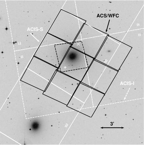
Figure 1.— Illustration of the 3x3 mosaic of our ACS observations (black solid lines) overplotted on a DSS-2 image of the NGC 1399 region. Also shown (black dashed polygon) is the FOV of the archival ACS observations covering the galaxy center. The white solid (dashed) lines outline the FOV of the Chandra ACIS-S (ACIS-I) chips with the aimpoint marked by the ’+’ (’X’) symbol.

The optical data were taken with the Advanced Camera for Surveys (ACS, Ford et al., 2003) onboard the Hubble Space Telescope (GO-10129), in the F606W filter with a total integration time of 2108 seconds per pointing. The observations were arranged in a $3\times 3$ ACS mosaic as illustrated in Figure 1. The individual observations were dithered to allow sub-pixel sampling of the ACS PSF and combined into a single image using the MultiDrizzle routine (Koekemoer et al., 2002). The final scale of the images is 0.03″/pix and provides a super-Nyquist sampling of the stellar point spread function with a full width at half maximum (FWHM) of $\sim\!0.09\arcsec$.

Table 1Photometric selection criteria for GC candidates

	blue GCs	red GCs
Ground-based	$T1<23$	$T1<23$
data	$1.0\leq C\!-\!T1<1.65$	$1.65\leq C\!-\!T1<2.2$
HST data	$z<22.5$	$z<22.5$
	$1.3\leq g\!-\!z<1.9$	$1.9\leq g\!-\!z<2.5$

To maximize the overlap with other observations (e.g. X-ray imaging and ground-based spectroscopy) the entire mosaic was centered on the coordinates: RA (J2000) $\!=\!03^{\rm h}38^{\rm m}28.62^{\rm s}$ and Dec (J2000) $\!=\!-35^{\rm o}28\arcmin\ 18.9\arcsec$. The field of view of the ACS mosaic covers $\sim\!100$ square arcminutes and extends out to a maximum projected galactocentric distance of $\sim\!50$ kpc with respect to NGC 1399, i.e. $\sim\!5.2$ effective radii of the diffuse galaxy light (de Vaucouleurs et al., 1991) and $\sim\!4.9$ core radii of the globular cluster system density profile (Schuberth et al., 2010).

Source catalogs were generated with SExtractor, using the appropriate weight maps produced by the Multidrizzle procedure, requiring a minimum area of 20 pixels and total S/N$>7$. The catalog astrometric solution was registered using the USNO-B1 catalog as a reference frame. Bright, unsaturated stars were identified in all ACS frames and matched with USNO-B1 sources obtaining a final accuracy of 0.2″ r.m.s.

Brightness estimates $m_{V}(F606W)$ in the STMAG photometric system for all detected sources were derived from isophotal magnitudes measured by SExtractor. While this approach is not optimal for resolved GCs, our accuracy is appropriate for the present work. Refined photometry for all GC candidates is computed in P11 in the VEGAMAG system, and compares well with our measurement, yielding an average conversion factor of $m_{\rm STMAG}-m_{\rm VEGA}=0.16$ mag at $m_{V}=23.5$ mag with a scatter of 0.04 mag.

Since no complete color catalog was available for the whole field, GC candidates were selected based on magnitude and morphological classification, choosing sources with SExtractor stellarity index $\geq 0.9$ and magnitude $m_{V}\!<\!26$ mag in order to exclude extended sources and compact background galaxies. The magnitude distribution of all point-like sources in our fields is shown in Figure 2. The distribution closely follows the GC luminosity function down to $m_{V}\!\lesssim\!26$ mag; at fainter magnitudes background unresolved sources dominate the number counts.

To include optical color information in our analysis we use the Bassino et al. (2006) $C-T1$ ground-based GC catalog, which contains data for $\sim\!50\%$ of our GC candidates within the HST FOV. Since the ground-based catalog is incomplete within 40″ from the NGC 1399 center due to galaxy light contamination, we included in our analysis the HST/ACS $g-z$ color catalog from Kundu et al. (2005) which provides colors for $\sim 90\%$ of GC candidates in the central region of the galaxy (see Figure 1). GCs were divided into blue and red populations as described in Table 1; note that the magnitude limit is chosen to ensure an approximately uniform completeness across the whole color and galactocentric distance range (Figure 13, also see Bassino et al. 2006).

In order to confirm the reliability of our GC selection method, based on single-band F606W photometry, and compare it with the color-selection usually adopted in the literature, we measure the fraction of GC candidates within the subset of sources with color information. Assuming that bona-fide GCs are represented by sources within the color ranges presented in Table 1, we derive two different estimates: i) for the central region covered by the more accurate $g$ and $z$ HST photometry and, ii) for the entire field covered by the ground based $C$ and $T1$ data. Within the central region $80\%$ of our GC candidates (within $m_{V}<26$ by definition) are consistent with the $1.3\leq g-z<2.5$ color cut; restricting the analisis to the bright subsample with $z<22.5$, used in the following sections to study the red and blue sub-populations, this number increases to $92\%$. Using the $C-T1$ photometry instead, which extends over the whole HST mosaic we find that $82\%$ of the GC candidates are consistent with the $1.0\leq C\!-\!T1<2.2$ color and $T1<23$ magnitude cuts. On the other hand, $\sim 4\%$ and $\sim 9\%$ of the GC candidates have respectively $g-z$ and $C-T1$ colors outside the allowed range as given in Table 1. We point out that using our stellarity selection criteria, we are able to effectively remove background galaxies since the fraction of such contaminants, which is expected to increase at large radii, varies by only by a few percent (from $7\%$ to $\sim 10\%$) across our entire FOV. Also note that in the following Sections we treat the $C-T1$ and $g-z$ subsamples separately when the different completeness levels may affect our conclusions.

To test whether very extended GCs are misclassified by our selection criteria, we estimated the completeness of our bona-fide GC sample as a function of GC size for the subset of optical sources with measured structural parameters (see $\S$ 3.5); in Figure 3 we show the effective radius distribution of the GC candidates samples, finding that our completeness drops below $50\%$ only for $R_{\rm eff}>5$ pc, with respect to color selected GCs. We also verified that relaxing the Stellarity index criterium does not increase the completeness for large ($R_{\rm eff}>5$ pc) GCs since these are fully resolved on our HST images, while increasing significantly the contamination level.

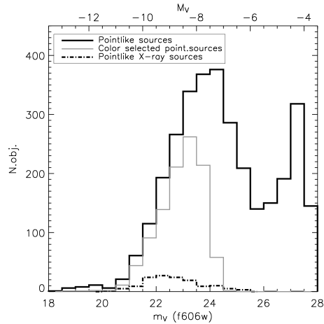
Figure 2.— Luminosity distributions of optical and X-ray point-like sources (e.g. with stellarity index $<0.9$) within the HST FOV. Also shown is the color-selected (Table 1) subsample of pointlike sources.

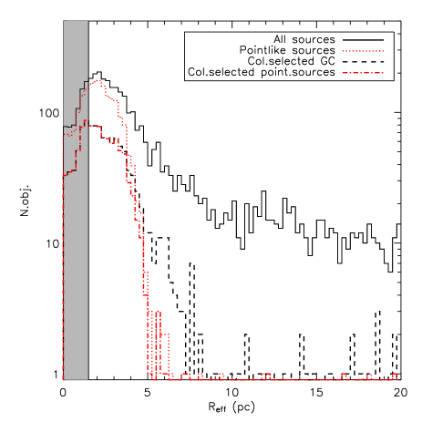
Figure 3.— Half-light radius distribution for the entire ACS optical catalog (solid line), compared to our GC candidates (dotted line). Restricting the sample to color-confirmed GCs (dashed and dot-dashed lines) shows that our selection criteria misses only very extended GCs with $R_{\rm eff}>5$ pc. The shaded region highlights the region where our size measurement are poorly constrained (see $\S$ 3.5).

2.2. Chandra X-ray data

The X-ray data were retrieved from the Chandra public archive. We selected observations #319 and #1472, i.e. two imaging datasets with the long exposure times where NGC 1399 lies close to the ACIS aimpoint, for a total exposure time of $\sim 100$ ks.

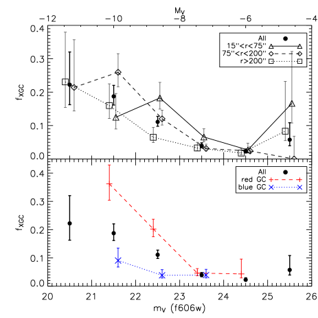
Figure 4.— Fraction of GCs hosting LMXBs as a function of luminosity. The two panels show parametrizations of those fractions by galactocentric distance (upper panel) or GC color (lower panel). The top abscissa gives the absolute magnitudes for the assumed Fornax distance of 20.13 Mpc (Dunn & Jerjen, 2006). The points are slightly shifted for visualization purposes.

The X-ray data were reduced with the CIAO software, extracting standard-grade events after applying bad pixel mask and afterglow corrections. The final exposure times, after removing high background periods, are shown in Table 2. To maximize the astrometric accuracy of the observations particular care was taken to correct for known offsets and to reproject the aspect solution and the event files of the individual observations using the NGC 1399 centroid as a reference point. In both cases the total offset was $<\!1\arcsec$. To minimize the uncertainties due to completeness variations over the FOV, we limited our analysis to the region in common to ACIS-I, ACIS-S and HST/ACS (see Figure 1). The subsequent analysis is thus limited to this overlap region.

Figure 5.— X-ray contours overlayed on ACS images: a very precise match (left), matched within 1″ (center) and X-ray source with no optical counterpart (right). The cross marks the X-ray centroid while the circle is our matching radius.

Table 2Journal of Chandra X-ray Observations

Obs.	Detector	Date	RA(J2000)	DEC(J2000)	$T_{\rm exp}$
#319	ACIS-S	2000-01-18	03h38m29.4s	$-35^{o}$27′00.4″	56 ks
#1472	ACIS-I	2003-05-26	03h38m25.6s	$-35^{o}$25′42.6″	45 ks

The wavdetect algorithm (Freeman et al., 2002) was used to obtain a preliminary source catalog for each dataset, using detection pixel scales of 1,2,4,8,16 and a significance threshold of $10^{-6}$. The registered observations were then aligned using the wavedetect catalogs with a residual positional uncertainty of 0.3″ r.m.s. and merged. Exposure maps were generated for both the individual observations and the merged dataset, and a merged source catalog was generated with wavdetect. In generating the X-ray catalogs the detection algorithm was run on both the whole $0.3\!-\!8$ keV energy band and on the $0.3\!-\!1$, $1\!-\!2$, $2\!-\!8$ narrow bands, finding $\sim\!12$ additional sources detected only in one of the narrow bands out of a total of 230 X-ray sources. For comparison with the literature, we note that 38 sources were not detected in the #319 dataset (cf. Angelini et al., 2001) and half of these were only detected in the merged dataset.

We used the ACIS Extract software (AE, Broos et al., 2010) to account for the variable PSF in the two X-ray datasets, as well as to improve the positional accuracy. AE uses library templates of the ACIS PSF to model the actual observed PSF for each observation, as well as for the composite one, allowing to derive source positions, properties and detection likelihood. We feed AE with the final source list derived from combining both individual and merged wavdetect catalogs. Each source was then inspected individually to check the position accuracy and to remove spurious objects due to poor data quality (very faint sources, high X-ray background in the field center, overlapping sources etc.), resulting in the removal of 3 objects, in agreement with the contamination expected based on the wavdetect significance threshold.

The AE software provides three different position estimates: input catalog, data centroid and correlation peak; our tests (as well as the AE manual) suggest that the ‘data centroid’ is the best estimate of the source position. Furthermore, we found that it is quite consistent with the wavdetect positions within $\sim\!0.1\arcsec$ except for the faintest objects and those farthest from the aimpoint where the difference can reach 0.5″. For three sources we decided to adopt the correlation peak which seemed a more reliable estimate after visual inspection; in any case, the difference between these estimates was always $<\!1\arcsec$. Finally the source catalogs were registered to the USNO-B1 reference frame using bright X-ray sources with optical counterparts (mostly GCs). The final accuracy of the X-ray catalog is 0.33″ with a maximum systematic offset of 0.6″.

The properties of the 230 X-ray sources in the composite Chandra/HST FOV are summarized in Table 4.

3. Analysis

3.1. Matching Optical and X-ray Data

To match the optical and X-ray sources we used the final catalogs registered on the USNO-B1 reference frame described in previous sections. Since the accuracy of the optical catalogs is $\sigma_{pos}^{opt}\simeq 0.2\arcsec$ while the X-ray one has $\sigma_{pos}^{X}\simeq 0.33\arcsec$, we adopted a conservative $2.5\sigma$ matching radius of 1″. Furthermore four sources, lying within the central 15″ of the galaxy, were excluded from the analysis because of the strong galaxy light contribution, both in optical and X-rays. Our matching algorithm thus yields 164 X-ray sources with optical counterparts, out of which 136 are matched with GC candidates. Note that 75% of these objects are matched within 0.5″. When multiple optical counterparts (usually 2) were present, i.e. for $\sim 14\%$ of the sample, we choose the closest one as the most likely match; however we verified that our conclusions do not change if we exclude such sources from our sample. While the matching accuracy is expected to depend on the galactocentric distance, mainly due to the larger Chandra PSF toward the outskirts of the ACIS FOV, we verified that even at large radii ($>2$ arcmin) doubling the matching radius results in a mild ($\sim 10\%$) gain in the number of matched sources, while increasing by $30\%$ the contamination level (see below). Our conservative choice thus minimizes the contamination at the cost of losing some of the fainter X-ray sources in the galaxy outskirts (cf. Figure 6). The properties of the closest optical counterpart for each X-ray source are reported in Table 4.

Adopting an optical source surface density ranging from 0.05 src/sq.arcsec in the central HST field, to 0.03 src/sq.arcsec in the southern field, the average chance of a random match with an X-ray source within our fiducial radius is $\sim\!12\%$, which drops to 4% considering only globular cluster candidates which have a factor $3\times$ lower surface density. Assuming a contamination of $\sim\!25$ background AGNs (Bauer et al., 2004), these figures result in NGC 1399 having a fraction of LMXBs residing in GCs of $f_{\rm GC-LMXB}=65\%\pm 5\%$, in good agreement with previous estimates (Kim et al., 2006; Angelini et al., 2001). This value, however, depends on galactocentric distance ranging from $\lesssim\!50\%$ within the central 50″ to 68% (77%) for $r\!>\!120\arcsec$ ($r\!>\!200\arcsec$).

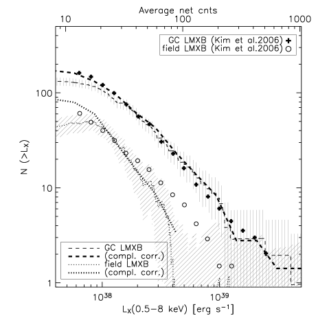
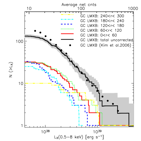
Figure 6.— Left panel: Cumulative X-ray Luminosity Function of GC and field LMXB. We observe a good agreement with Kim et al. (2006, arbitrarily re-normalized) for GC-LMXB, while our LF for field LMXB is marginally steeper (see discussion in text). The shaded region represent $1\sigma$ errors. Right panel: X-ray luminosity function in different radial bins.

X-ray sources tend to reside in compact bright optical counterparts, i.e. bright GCs (Figure 2): only 28 out of 164 objects ($17\%$) are in fact associated with extended sources. The fraction of GCs hosting an X-ray source ($f_{XGC}$) drops with magnitude from $\sim\!20\%$ to $2\%$ and depends on radial distance and color of the host GC (Figure 4). The drop in the brightest magnitude bins is due to a combination of the different radial profile of the red and blue GC populations ($\S$3.4) coupled with the lack of bright red GCs, compared to the blue population, in particular in the galaxy center (cf. Figure 13). We do not observe any significant difference in $f_{XGC}$ in the red and blue sub-population as a function of radius when also splitting in luminosity bins, although our sample is too small to draw definitive conclusions. In any case we stress that this interplay between GC galactocentric distance, magnitude, and color must be taken into account in studies observing only the central regions of galaxies.

Finally note that these results are affected relatively little by our GC selection criteria, since the majority of X-ray sources matched to an optical counterpart reside in compact objects (see $\S$3.5): even considering that we may be missing part of the most extended GCs (see $\S$2.1), this would result in a lower $f_{XGC}$ by a few percent and anyway within the statistical uncertainties.

3.2. The X-ray Luminosity Function

For each X-ray source in our catalog, the ACIS Extract procedure (see §2.2) computes the incident photon flux, applying the quantum efficiency and spectral response corrections (i.e. using the ARF and RMFs) appropriate for each observation at the specific detector location, which are then combined in a final weighted average. This ensures that the position and time dependence of the ACIS efficiency is properly taken into account.

The X-ray luminosity function (LF) of LMXBs in NGC 1399 was obtained applying an average conversion factor to the photon fluxes measured by AE, computed assuming a power-law spectrum with $\Gamma=1.5$ and a Galactic column density of $1.3\times 10^{20}$ cm^-2, which corresponds to the spectral model for our average source (Figure 10). To correct for contamination due to background sources we used the AGN number counts of Bauer et al. (2004). The cumulative LF of both GC- and field-LMXBs, shown in Figure 6 (left panel), has a power-law shape down to $\sim 2\times 10^{38}$ erg s^-1. At fainter fluxes the combined effect of incompleteness and source variability may affect the LF shape. To correct for incompleteness, due to the variable PSF over the FOV and the diffuse X-ray emission, we adopted the “forward” procedure described in Kim & Fabbiano (2003), accounting for the effect of background, source counts and distance from the aimpoint. The detection probabilities as a function of source number counts, at various off-axis angles, are shown in Figure 7.

Figure 7.— X-ray detection probabilities as a function of the off-axis angle and the number of counts detected in a given source. This grid has been calculated following the ”forward” procedure described in Kim & Fabbiano (2003). Such probabilities are used to correct for incompleteness (in e.g. LFs, radial profiles) due to the diffuse X-ray background and variable PSF.

Since X-ray binaries are intrinsically variable, finite integration times may influence their detectability. Moreover, the effect of variability on stacked observations may change the LF slope close to the completeness limit of the individual observations, as discussed in detail by Zezas et al. (2007). We verified that the LF of the individual Chandra observations (#319 and #1472) are consistent within the statistical uncertainties, except for the somewhat shallower completeness limit due to the shorter exposure time.

The completeness corrected GC-LMXB LF follows a power-law down to $f_{X}\lesssim 10^{38}$ erg s^-1 with a differential slope of $-1.7\pm 0.2$ in the $0.8-5\times 10^{38}$ erg/s range, in good agreement with the one derived by Kim et al. (2006) from a sample of six early-type galaxies. Some residual incompleteness can be observed in the faintest bins ($\lesssim\!10-20$ counts) mainly due to the very high background in the galaxy center. In fact splitting the LF in radial bins (Figure 6, right panel) shows that the intermediate bin (120″-180″), which covers the range of maximum completeness (Figure 7) does not deviate significantly from a power-law down to $10^{38}$ erg s^-1 and below. The GC-LMXB LF in the outermost radial bin presents an excess of bright ($L_{X}\!>\!5\!\times\!10^{38}$ erg s^-1) sources with respect to the inner regions of the galaxy, suggesting that there may be some residual contamination from background sources in the galaxy outskirts. In fact only one X-ray source is detected at $L_{X}>10^{39}$ erg s^-1 in the color-selected GC sample (see below).

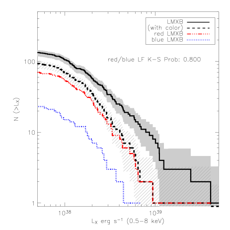
Figure 8.— Dependence of the cumulative GC-LMXB X-ray luminosity function on the color of their host GCs. The K-S probability that red and blue LMXBs are drawn from the same parent population is also shown, indicating that the two LFs are statistically indistinguishable.

We do not detect any significant difference in the cumulative LF as a function of the host GC color. Figure 8 shows that the LFs of red and blue GC-LMXB are statistically indistinguihable according to a K-S test, and that they are consistent with the global LF except at the very bright end. For $L_{X}\!>\!10^{39}$ erg s^-1, two sources included in the GC-LMXB LF in Figure 6 have no color information, while other three X-ray sources associated with compact optical counterparts have colors outside the selected range (Table 1) and thus likely represent interlopers.

Our field-LMXB LF is somewhat steeper than the literature estimate, altough consistent within the errors, with a differential slope of $-2.5^{+0.7}_{-1.4}$ in the $0.8-5\times 10^{38}$ erg/s range. Furthermore it suggests a lack of bright LMXBs above $L_{X}\gtrsim 3\!-\!4\times 10^{38}$: assuming for field LMXBs the same underlying distribution as observed for GC-LMXBs, and considering that we have about twice as many LMXB in GC than in the field, the probability of observing no field source above $5\times 10^{38}$ erg/s is $\sim 1\%$, incresing to $\sim 5\%$ if we allow for cosmic variance in the AGN number counts (which dominate at bright fluxes) by a factor 2. We find that this significance does not depend on galactocentric distance, and is also confirmed when analyzing the individual X-ray observations #319 and #1472 separately.

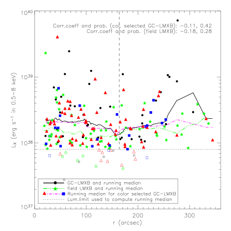
Figure 9.— LMXB luminosity as a function of galactocentric distance. Triangles and squares represent the red and blue GC-LMXB respectively, while field LMXB are marked by stars. The solid symbols are those used to compute the running average of each subsample, using the uniform completeness limit marked by the dotted line. We find that in the galaxy center GC-LMXB are significantly brighter than field LMXBs, although we don’t detect the correlation with galactocentric radius reported by Fabbiano et al. (2010, see discussion in text) for NGC 4278. The vertical dashed line marks the distance limit adopted for the correlation tests, corresponding to the distance limit probed by Fabbiano et al. (2010).

The LMXB X-ray luminosity is shown in Figure 9 as a function of galactocentric radius. There is some evidence that the median GC-LMXB X-ray luminosity is larger than for field LMXBs, at least in the galaxy center within $r<160$ arcsec, in agreement with the flatter LF observed for GC-LMXBs. At larger radii the difference disappears but here the smaller number of sources and the background contamination, which affects mainly field LMXBs, makes any conclusion tentative. To check that this difference is not the result of a sampling effect due to the fact that we are observing about twice as many GC- than field-LMXBs, we performed 1000 simulations, randomly resampling our LMXB sample, while preserving the relative ratio of the two populations. We find that the likelihood to obtain the median difference that we observed is $\sim 2\%$.

This result is in agreement with what is observed by Fabbiano et al. (2010) in NGC 4278: in that galaxy the authors find an anti-correlation between the GC-LMXB X-ray luminosity and galactocentric distance, in the sense that GC-LMXB are brighter closer to the galaxy center, and brighter on average than field sources. In NGC1399 however a Spearman Rank test, within $160$ arcsec, does not yield any significant correlation (see Figure 9) between X-ray luminosity and galactocentric distance, as can be expected given the large scatter in $L_{X}$.

3.3. X-ray Spectral Properties and Variability

We test whether we can detect any dependence of the X-ray spectrum of LMXBs on the presence of a host GC or on the color of the host GC itself. For this we compare the $0.5-1$ vs $1-2$ keV (HR1) to the $0.5-1$ vs $2-8$ keV (HR2) hardness ratios, finding that field-LMXBs, as well as red and blue GC-LMXBs, span a similar range of X-ray colors, consistent with either a Bremsstrahlung or power-law spectral model (see Figure 10). A 2D K-S test confirmed that there is no significant difference in the hardness ratio of these LMXB populations.

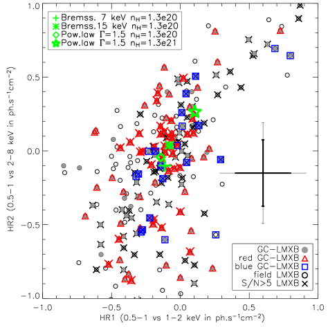
Figure 10.— HR1-HR2 X-ray color-color diagram for field- and GC-LMXBs. Red and blue solid circles represent LMXBs hosted by red and blue GCs respectively, while black symbols are GC-LMXB without color informations. The crosses mark sources with high-quality data ($S/N\!>\!5$). We overplot the predictions from different spectral models and variable absorption: a Bremsstrahlung with $kT=7-15$ keV, or a power-law model with $\Gamma=1.5$ and column density $n_{H}=1.3\times 10^{20}$ are all consistent with the bulk of the population, while a higher column density of $n_{H}=1.3\times 10^{21}$ produces a shift of $\sim 0.3$ toward the upper-right corner of the plot. The typical error for all (thin line) and high-quality (thick line) data is shown on the right.

We investigate the time variability of X-ray sources both within each observation through Kolmogorov-Smirnov testing, and across observations, comparing the error-weighted fluxes at the two epochs. We detect variability in 30 X-ray sources (see Table 4), 13 of which residing in color selected GCs. The fraction of variable sources increases from $\sim\!10\%$ below $3\!\times\!10^{38}\,\mbox{erg s}^{-1}$ up to $\sim\!33\%$ for $3\!\times\!10^{38}\!<\!L_{X}\!<\!10^{39}\,\mbox{erg s}^{-1}$, as expected by the better photon statistics, while it remains constant at $\sim\!14\%$ as a function of the host GC optical magnitude. While these results suggest that bright X-ray sources in GCs are not simply due to the superposition of several low luminosity binaries, we cannot exclude, based only on temporal analysis, that some GC host multiple LMXBs, since the observed variability can be easily accounted for if, e.g., a bright source dominates the LMXB population within a GC.

On the other hand in the only color-confirmed GC-LMXBs (source no.141 in Table 4) with $L_{X}>10^{39}\mbox{erg s}^{-1}$, we do not detect any sign of variability despite the $S/N>20$. To test the statistical significance of this result we extracted from the RXTE archive the Mission-Long lightcurve of the Galactic BH binary GRS1915+105. After degrading the data to the same S/N level of our source, we find that the likelihood of finding a difference of less than 3% in flux between 2 observations obtained 3.3 yrs apart, as for NGC1399, is only $\sim 3\%$.

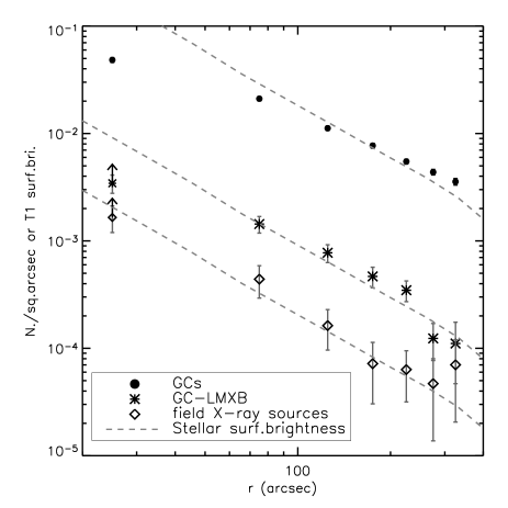
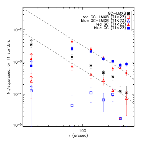
Figure 11.— Radial surface density profiles of GCs and LMXBs. The dashed lines represent the T1 surface brightness profile of the diffuse galaxy light, taken from Dirsch et al. (2003) and arbitrarily rescaled. GC-LMXBs tend to follow the parent GC population, while field LMXBs are closer to the galaxy light distribution.

3.4. LMXB/GC connection: Spatial distribution

As already discussed in $\S$3.1 the fraction of LMXBs hosted in GCs changes with galactocentric radius, indicating different spatial density distributions of field- and GC-LMXBs. In Figure 11 we plot the radial profiles of the optically identified GC population, the GC-LMXBs and field X-ray sources. Incompleteness effects in the LMXB profiles have been corrected as described in previous sections, except for the central bin which represents a lower limit since the high level of diffuse emission makes the correction uncertain. As indicated by other studies (e.g. Dirsch et al., 2003; Puzia et al., 2004; Bassino et al., 2006; Schuberth et al., 2010) the GC population is more extended than the galaxy light. A similar behavior is found for LMXBs hosted in GCs (even though with less significance due to the smaller sample statistics) while the field X-ray sources have a steeper profile close to the one of the diffuse galaxy light. Note that the surface density of GCs within the central 50″ is lower than expected from a simple power-law extrapolation of the external GC distribution. This is not an incompleteness effect since it is present even when only the brightest GCs are taken into account, and is in agreement with the shallower central profile observed by Dirsch et al. (2003), Bassino et al. (2006), and Schuberth et al. (2010). Thus, while the difference between GC and field LMXBs is mostly due to the central region of the galaxy ($r<50``$) where the completeness corrections are more uncertain, the fact that the GC-LMXB surface density profile presents a similar deficit of sources in the central bin, while field-LMXBs show no such behaviour, supports the view that this difference is not due to incompleteness effects.

In Figure 11 (right panel), we further divide the GC population according its $C\!-\!T1$ color (see Table 1). In this case the incompleteness of the color catalog is clearly visible within the central bin, as discussed in $\S\ref{opt_data_sect}$. However, the plot shows that the shallower GC distribution is mainly due to the blue GC component (see also Schuberth et al., 2010). When compared with GC-LMXBs we find no significant difference between the LMXB distribution and the one of the host GC population.

These results are confirmed by the cumulative distributions in Figure 12: while the GC and GC-LMXB profiles are consistent with each other (upper panel), the field-LMXBs are much more concentrated than GCs at $>99.9\%$ confidence level according to a K-S test. Furthermore, the blue GC sub-population is more extended than the red one (Dirsch et al., 2003). However, LMXBs seem to follow the distribution of their host GCs, with little evidence of the more extended distribution found by Kim et al. (2006). Figure 12 also shows that incompleteness effects in the X-ray source distribution do not significantly affect these conclusions.

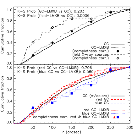
Figure 12.— Upper panel: Cumulative surface density profiles of GCs and LMXBs. The low K-S test probability reported in the figure confirms that field LMXBs have a different radial distribution from the GC population. Lower panel: Cumulative profiles of GCs and LMXBs with available color informations. Both red and blue GC-LMXBs are distributed according to their host GC population. In both panels the points show that incompleteness effects do not affect the results.

This behaviour is also seen in the color-magnitude diagrams shown in Figure 13: not only do the LMXB-host GCs become bluer toward the galaxy outskirts, but the overall GC population shifts toward bluer colors. In addition, we see the presence of a very red GC population ($C-T1\!\approx\!2.15$ mag or $g-z\!\approx\!2.2$ mag), already noticed by Kundu et al. (2007), which resides in the NGC 1399 core and hosts the majority of red LMXBs. The fraction of red and blue GCs hosting LMXBs is shown in the plots. We can see that both red and blue GCs have a constant frequency within the errors, as expected if LMXBs follow the distribution of their host GCs. While the mild decrease observed in the red population in the outermost bin is marginally consistent with the trend reported by Kim et al. (2006), the LMXB frequency within the blue population shows the opposite trend, inconsistent with the large drop ($\gtrsim\!2$) predicted by these authors.

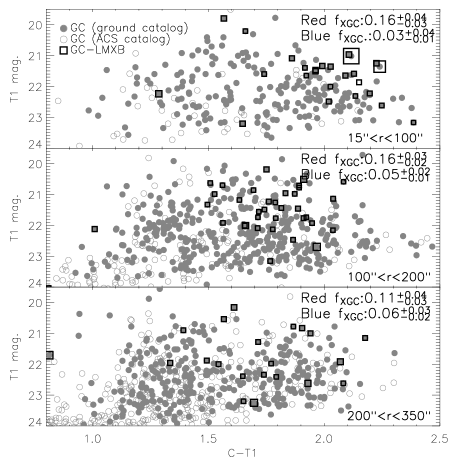
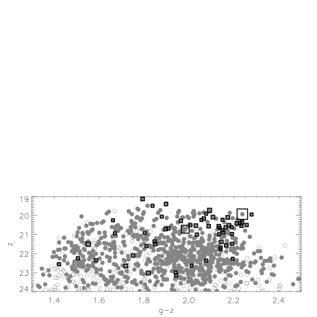
Figure 13.— Color-magnitude diagrams using $C\!-\!T1$ ground-based (upper panel) and $g\!-\!z$ HST photometry (lower panel). Ground-based plots are split according to galactocentric distance, while HST data refers to the whole ACS field ($\sim\!200\arcsec\!\times\!200\arcsec$). Open grey dots represent sources in color catalogs while solid ones refer to GC candidates detected in our F606W ACS data. Black squares indicate GC hosting LMXBs, where the symbol size proportional to the $\log$ of the X-ray flux in the $0.5\!-\!8$ keV band. The fraction $f_{XGC}$ of color-selected GCs hosting X-ray sources, reported in the upper panel, shows no dependence on galactocentric distance.

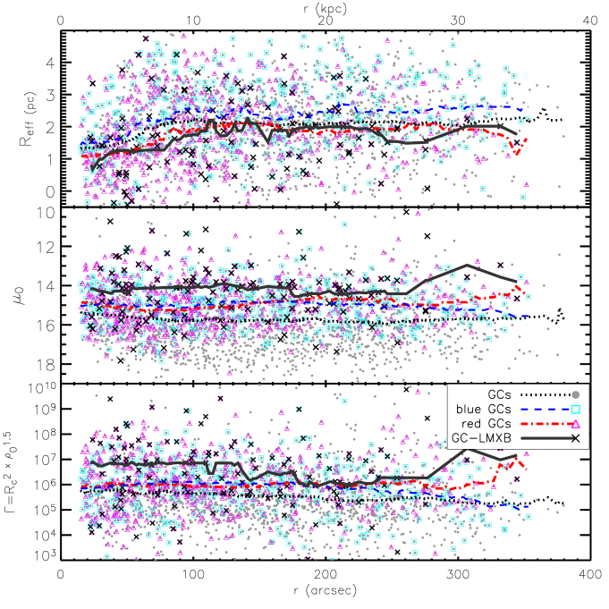
Figure 14.— Galactocentric dependence of GCs structural parameters. GCs and color-selected sub-populations are shown in grey dots, red triangles and blue squares, respectively. GCs hosting LMXBs are marked by black $\times$. The running median values (solid and dashed lines) show that the different populations have different structural parameters.

3.5. The LMXB/GC Connection: GCs Structural Parameters

Structural parameters were measured, as explained in detail in P11, using the GalFit software (Peng et al., 2002) to fit a King (1962) model to our HST data, including the error maps produced by the Multidrizzle routine as weight maps, we derived tidal, core and effective radii, and central surface brightness values.

Typical GCs are marginally resolved at the distance of NGC 1399, hence accurate knowledge of the PSF is crucial to derive robust GC structural parameters. As discussed in detail in P11, we designed a specific software, the Multiking package which makes use of the empirical PSF library for ACS/WFC (Anderson, 2005; Anderson & King, 2006) to build a new drizzled PSF library replicating the actual data frame properties (orientation, dither pattern, astrometry, etc.) in order to account for all effects related to the observing strategy and data reduction process.

The accuracy of our measurements was estimated using several thousand simulated GCs produced with the Multiking package to include all instrumental effects (field distortions, PSF variation, etc.). We used the simulated GC catalog to correct for residual systematics affecting the structural parameters measurements, by fitting a polynomial function to the measured values as a function of the input value, and applying such correction to the real GC measurements. While we refer the reader to P11 for a comprehensive discussion of the fitting accuracy, our simulations show that we can robustly measure the individual effective (i.e. half-light) GC radius in the range $\sim\!1.5\!-\!20$ pc with an average uncertainty of $0.56$ pc and little dependence on magnitude, background level or galactocentric distance. We also emphasize that our bona-fide GC sample has an integrated $S/N>100$, in good agreement with the minimum prescription of Carlson & Holtzman (2001) to measure sizes of marginally resolved GCs.

In the top panel of Figure 14 we show the galactocentric dependence of the half-light radius. In the central 50″ the distribution is dominated by a very compact GC population, which also hosts the majority of LMXBs. An increase of the GC effective radius with galactocentric distance has originally been observed in the Milky Way (van den Bergh, 1991) and later in several other massive early-type galaxies (e.g. Spitler et al., 2006; Madrid et al., 2009; Harris, 2009, and references therein). In NGC 1399 the projected size gradient seems to be mostly confined to the inner core ($\lesssim\!100\arcsec$), and remains approximately constant outside $\gtrsim\!1\,R_{\rm eff}$ out to $\sim\!5\,R_{\rm eff}$ of the diffuse galaxy light, similar to what was found by Spitler et al. (2006) in the Sombrero galaxy. However, at odds with the latter work, we find the same behaviour for both red and blue subpopulations even at large radii, arguing in favor of an intrinsic difference and against projection effects (see also $\S$4.2). This may suggest the presence of a lower threshold in radius below which tidal forces allow the survival of most compact stellar systems and further supports the need to reach larger galactocentric distances than probed by most high spatial-resolution HST studies of extragalactic GCs, since the very central regions of giant galaxies do not necessarily reflect the properties of the entire GC population.

We find that GCs hosting X-ray sources (XGC) are, on average, more compact that the rest of the GC population, but do not differ significantly form the red GC population which hosts the majority of LMXBs. This is clear from looking at the cumulative distribution of the GC effective radius shown in Figure 15: while red and blue GCs have different sizes at a significance level $>\!99\%$, we cannot detect any significant difference between red XGCs and the overall red GC sub-population. On the other hand, LMXBs residing in blue GCs seem to prefer the most compact systems, even though this difference is only significant at the $2\sigma$ level. This indicates that more than one physical parameter is driving LMXB formation.

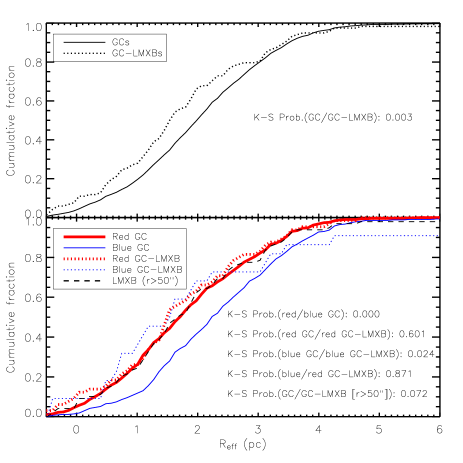
Figure 15.— Cumulative distributions of GC effective radii. The upper panel illustrates the distributions for GCs with and without LMXBs, while the lower panel shows the corresponding distribution for the blue and red GC sub-populations, as well as all LMXB sources. The K-S test results, reported in the plot, show the probability of different subsamples to be drawn from the same parent distribution: GC-LMXBs are more compact than the bulk of the GC population, but are similar to the red GC subpopulation.

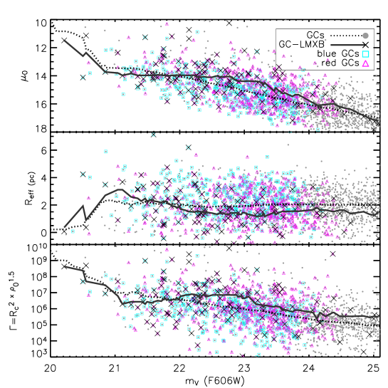
Figure 16.— Structural parameters versus GC magnitude. Solid circles represent GCs, while crosses indicate LMXBs. The solid and dashed lines represent the running median of the GC-LMXB and GC distribution, respectively. LMXBs tend to have different structural parameters from the GC population, except at bright magnitudes.

The middle and bottom panels of Figure 14 show the $V_{\rm F606W}$-band central surface brightness $\mu_{0}$, and the interaction rate $\Gamma=R_{\rm c}^{2}\rho_{0}^{1.5}$ (see e.g. Verbunt & Lewin, 2006), as a function of galactocentric radius. The Figure indicates that LMXBs are preferentially hosted by high central surface brightness and/or high interaction rate GCs at all galactocentric radii, independent of the host GC color. This behaviour, however, is due in part to the tendency of LMXBs to reside in bright GCs discussed in §3.1. To understand whether GC structural parameters have an effect on LMXB formation likelihood in addition to luminosity and metallicity, we plot the main parameters against GC luminosity in Figure 16 and against GC color in Figure 17. While it is difficult to disentangle the effect of each parameter since they are correlated through the definition of the King profile, LMXBs residing in intermediate-luminosity and faint GCs ($m_{V}\!>\!22$) have a higher central surface brightness, smaller effective radius and larger encounter rate than the average GC population. However, at variance with other studies (e.g. Peacock et al., 2009) this difference disappears for the brightest GCs.

Figure 17 shows that GC color has an intrinsic effect on the LMXB formation likelihood, since blue GCs appear deficient in LMXBs even though they have similar central surface brightness and interaction rates as the red ones, except perhaps for very blue colors ($C\!-\!T1\!<\!1.3$ mag). We conclude that the different fraction of LMXBs observed between the red and blue GC sub-population cannot be attributed to differences only in their structural parameters, thus, supporting the view that stellar evolution (Grindlay, 1987; Maccarone et al., 2004; Ivanova, 2006) and/or mass segregation effects (Jordán et al., 2004) must influence LMXB formation.

To quantify the likelihood that GC structure has an impact on LMXB formation, in addition to luminosity and color, we resampled the photometric GC dataset to match the XGC optical luminosity and $C-T1$ color distribution. We generated 10000 resampled distributions testing through S- and T-statistics whether the mean and variance of the resampled dataset is equivalent to the reference XGC distribution. Table 3 summarizes the probabilities of obtaining the same median for the LMXB and non-LMXB GC population for a given GC parameter. This Monte-Carlo exercise shows that XGCs tend to have significantly ($P\gtrsim 99\%$) larger $\Gamma$ and smaller $R_{\rm eff}$ than the parent GC population even after removing the luminosity (mass) and color dependence. Similarly, by resampling according to the XGC distribution in either $\mu_{0}$ or $\Gamma$ and color, we find that GCs hosting LMXBs are more likely to be brighter than the rest of the GC population, indicating that the GC mass seems to play a role even after removing the dependence on the other GC parameters. This is partially at odds with the findings of Jordán et al. (2007a) in the Cen-A GC system, where mass does not seem to play a significant role in LMXB formation, but can be explained from the comparison shown in Figure 16 where structural parameters of XGC are significantly different from the whole GC population only at faint ($m_{V}\gtrsim 22$) magnitudes while at the bright end this difference disappears.

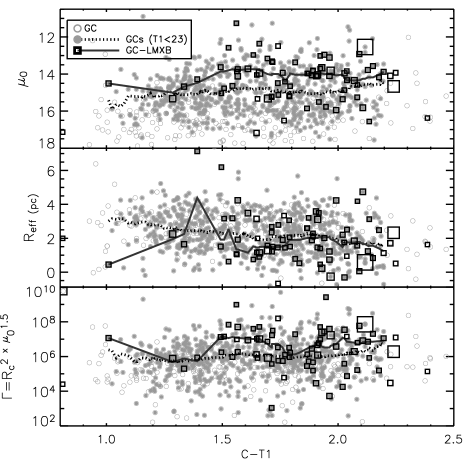
Figure 17.— Structural parameters versus GC color. Grey solid (open) circles represent GCs above (below) the magnitude thereshold of T1=24 used for the color-selected subsample of Table 1, while LMXBs are marked by black squares whose size is proportional to the logarithm of their X-ray luminosities. The solid and dashed lines represent the running median of the GC-LMXB and GC distribution, respectively.

Table 3Two-parameter resampling probabilities

Resampled in	P($m_{V}$)	P($\mu_{0}$)	P($\Gamma$)	P($R_{\rm eff}$)
$m_{V}$, C–T1 color	$\cdots$	0.26	0.001	0.01
$\mu_{0}$, C–T1 color	0.003	$\cdots$	0.16	0.22
$\Gamma$, C–T1 color	0.002	0.04	$\cdots$	0.39

Note. — The values represent the probability of obtaining the same median for the LMXB and non-LMXB GC populations, after resampling the non-LMXB sample according to the probability density distribution of the two quoted parameters. See text for details.

4. Discussion

Our analysis confirms the result, first reported by Angelini et al. (2001, see also ), that NGC 1399 has the highest global fraction of LMXBs hosted by GCs ($f_{\rm GC-LMXB}$) among early-type galaxies studied so far, with $f_{\rm GC-LMXB}=65\%\pm 5\%$. We also find however that $f_{\rm GC-LMXB}$ increases with galactocentric distance, ranging from $\sim 50\%$ within 50″ ($\sim 5$ kpc) to $>75\%$ at $r>200\arcsec$ ($\gtrsim 20$ kpc). While the exact value of $f_{\rm GC-LMXB}$ is affected by large uncertainties, in particular near the center of the galaxy due to the high X-ray background, an increase of $f_{\rm GC-LMXB}$ with galactocentric distance is in agreement with the fact that the radial distribution of GCs in NGC 1399 is more extended than the galaxy light, while field LMXBs tend to follow instead the galaxy surface brightness profile ($\S$ 3.4). Thus, some care must be taken when comparing different $f_{\rm GC-LMXB}$ estimates, sampling different galactocentric distances. In this respect we note that our result suggests a lower central $f_{\rm GC-LMXB}$ than the one measured by Angelini et al. (2001, $f_{\rm GC-LMXB}\sim 70\%$).

While $f_{\rm GC-LMXB}$ is known to depend on GC specific frequency $S_{N}$ (Maccarone et al., 2003; Sarazin et al., 2003; Juett, 2005), NGC 1399 has a large $f_{\rm GC-LMXB}$ even after taking into account its high $S_{N}$. Our results suggest that this galaxy is only marginally consistent (at the $3\sigma$ level) with the $\sim 50\%$ value found for galaxies with similar $S_{N}$ by Kim et al. (2006), such as NGC 4649 or NGC 4472 (see their Figure 15). This difference is not affected by the intrinsic radial gradient in the GC-LMXB distribution, since the Kim et al. (2006) study used wide-field ground-based data covering a galaxy fraction similar to our work; furthermore, if the Kim et al. (2006) GC sample is contaminated by background galaxies (hosting an X-ray source), the actual $f_{\rm GC-LMXB}$ will be lower than observed by these authors thus strengthening our conclusion. Its significance, however, also depends on the probed X-ray luminosity range, as discussed further in $\S$4.1.

On the other hand, on average $\sim\!6\%$ of GCs with $m_{V}\!<\!26$ ($M_{V}\!<\!-5.5$) host LMXBs; while this number is consistent with the average value for early-type systems reported in literature (see Fabbiano, 2006, and references therein), we point out that the exact value depends on the studied magnitude range (Figure 4) and, to a lesser extent, on galactocentric distance (Figure 13). In particular our data allow us to probe the GC population $\sim 2$ magnitudes below the LF turnover, while most studies based on color selected samples are limited to the bright LF end (Fig. 2). LMXBs are preferentially hosted by bright ($m_{V}\lesssim 24$) and red GC with fractions $f_{XGC}$ that can be $>20\%$ (Figure 2 and 4). This value is almost twice as large as the one found in similar early-type galaxies by, e.g., Kim et al. (2006); the depth of the X-ray data can only account for part of this difference since i) our completeness limit is comparable to the one of the combined LF of the Kim et al. (2006) sample and ii) we have $<30\%$ more X-ray sources in the merged dataset than in the #319 observation used by the latter authors for NGC1399 (see $\S$ 2.2). On the other hand the observed difference could be explained if the ground-based data are significantly contaminated by background sources, which would lower $f_{XGC}$ measured by Kim et al. (2006).

Red GCs are $\gtrsim 3$ times more likely to host an LMXB than blue GCs, in agreement with the results of Kundu et al. (2007). We confirm the presence of a very red GC population which hosts most LMXBs in the galaxy center (Figure 13), as reported by Kundu et al. (2007), and which is better visible using the larger $g\!-\!z$ color baseline of the ACS dataset. However this population seems to disappear at larger galactocentric distances, where the overall GC population, including those hosting LMXBs, moves toward bluer colors. While the presence of a similar very red sub-population was not observed in the other 4 galaxies studied by the latter authors, a more homogeneous dataset probing large galactocentric distances, is needed to address the problem of the universality of such feature and its role in LMXB formation.

4.1. Insights from the LMXB Spatial Distribution

Studies of the radial distribution of LMXBs in the past yielded apparently contrasting results. For instance, Kim & Fabbiano (2003) and Humphrey & Buote (2004) found that LMXBs follow the host galaxy light distribution in NGC 1316 and NGC 1332, while in NGC 4472 Kundu et al. (2002) find that LMXBs follow the GC distribution better than the optical light. Also, Sarazin et al. (2003) and Jordán et al. (2004) found no difference between the distribution of field- and GC-LMXBs, while Kundu et al. (2007) observe that field-LMXBs are more centrally concentrated than GC-LMXBs. We note, however, that an accurate comparison of these results is hampered by the different spatial resolutions and galactocentric ranges covered by these studies. Furthermore, the interplay between the spatial and color distribution of the GC sample may explain the discrepancies, since blue and red GCs have different radial distributions and host different fractions of the LMXB population.

In the case of NGC 1399, we find that the radial distribution of field-LMXBs out to $\sim\!5.2\,R_{\rm eff}$ of the diffuse galaxy light, is significantly steeper than GC-LMXBs, with a statistical significance $>99.9\%$, in agreement with the results of Kundu et al. (2007) for a sample of five early-type galaxies, however, with smaller galactocentric coverage. This result supports the conclusion that field LMXBs are not likely to be formed in GCs and later expelled by three- and four-body interactions, as proposed by e.g. White et al. (2002), since in such a case field- and GC-LMXBs would be expected to have similar radial surface density profiles. Field LMXBs (Figure 11, left panel) follow, in fact, the surface brightness of their host galaxy, suggesting an evolutionary connection to the main stellar body of the galaxy rather than to GCs. GC destruction has been proposed as an alternative mechanism to produce field LMXBs; in this scenario the increased strength of tidal fields in the galaxy core would result in a field LMXB distribution more centrally concentrated than the one of their parent GC population if they were preferentially formed in GCs that moved through the galaxy core regions. The effect of the tidal field of the host galaxy on the GC population is possibly observed in the $\sim\!20\%$ smaller sizes of the total GC populations (blue and red GCs) within the central 10 kpc ($100\arcsec$, see P11). Note, however, that given the low fraction of GC-hosting LMXBs and its dependence on the host GC color, the production of all field LMXBs in GC requires the disruption of a very large fraction of stellar systems, and a very finely tuned interplay between the original host GC system, color and spatial distribution to reproduce the observed distributions.

On the other hand, we do not detect any significant difference between the GC-LMXB distribution and the overall GC distribution, at odds with the result of Kim et al. (2006) that both red and blue GC-LMXBs have steeper profiles than blue and red GC populations. Our data suggest that LMXBs hosted by red GCs simply follow their parent distribution; the statistics are too low for blue LMXBs to draw significant conclusions, but we note that an opposite trend is found with LMXBs in blue GCs having a shallower number surface density profile around NGC 1399 than the corresponding blue GC sub-population. It is possible that the Kim et al. (2006) result is affected by contamination issues at large radii due to the lower spatial resolution of their ground-based data, as well as the fact that NGC 1399 has different properties than the other galaxies included in their sample.

The conclusion that field LMXB follow a different formation path from GC-LMXB in supported by the results of Kim et al. (2009), based on the analysis of HST and Chandra data of 3 nearby ellipticals, showing that the abundance of field LMXBs does not depend on the GC specific frequency $S_{N}$ as strongly as observed for GC-LMXB. To compare NGC 1399 with the sample of Kim et al. (2009) we calculated the number of field and GC LMXBs within $D_{25}$, as reported by RC3, normalized by total K band luminosity; since Kim et al. (2009) reach fainter X-ray luminosities ($L_{X}>10^{37}$ erg/s) than probed by our data, we extrapolated our LF down to the same limit using the different LF fits proposed by the latter authors, consisting in either a single or broken power-law, obtaining correction factors ranging from 1.6 up to 2.3. The NGC 1399 GC specific frequency was calculated within the same region (since $S_{N}$ is known to depend on galactocentric distance, Dirsch et al., 2003, see e.g.), and turns out to be $\sim 30\%$ lower than the global value of 5.1 usually reported in literature. The result, shown in Figure 18, supports the difference between GC and field LMXB population, with the former more strongly dependent on $S_{N}$. The claim that NGC 1399 has an unusually rich LMXB population, down to such faint X-ray luminosities, depends critically on the assumed LF correction: while using the average correction term would support the peculiar nature of NGC1399, if the faint end of the GC-LMXB LF is flatter than the field one the NGC1399 GC-LMXB population would be comparable (lower errorbar limit in Figure 18) within the statistical uncertainties to the one of NGC4278. We speculate that, if confirmed, the very red GC subpopulation (see $\S$3.4) could be responsible for part of this difference given the strong effect that metallicity has on LMXB formation; we also point out that although all galaxies used for this plot are giant ellipticals, only NGC 1399 is a central cluster cD galaxy.

On the other hand, our results point toward a number of field binaries consistent with those of poorer GC systems implying that only a small fraction of LMXB is likely to have escaped from their host GC.

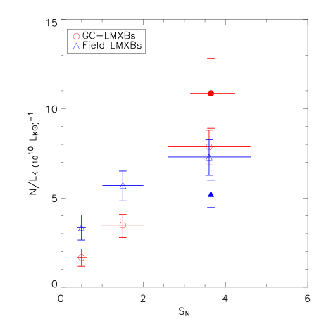
Figure 18.— Number of LMXBs (normalized to galaxy K band luminosity) as a function of specific frequency $S_{N}$. Empty symbols represent the Kim et al. (2009) dataset, i.e. from left to right NGC 3379, NGC 4697 and NGC 4278, while solid ones represents the values for NGC 1399 derived in this work. All values were calculated within $D_{25}$ and excluding the central 10” region; the errorbars for NGC1399 include both statistical and systematic uncertainties due to the use of different X-ray LF (see discussion in text). The GC-LMXB abundance is more strongly dependent on $S_{N}$ than for field source, supporting different evolutionary paths of the two populations.

4.2. The Influence of GC Structure on LMXB Formation

Our analysis of the structural properties of GCs hosting LMXBs (XGC) confirms the results of previous studies that focused on the core regions of early-type galaxies (Jordán et al., 2004, 2007a; Sivakoff et al., 2007), which found that LMXBs are preferentially formed in the most compact GCs. The XGC size distribution is, however, similar to the one of the red GC sub-population and is $\sim\!20\%$ more compact than the blue GC sub-population. Thus, we cannot exclude with certainty that the observed size difference reflects differences in the parent GC population. Spitler et al. (2006), in their study of the Sombrero galaxy (NGC 4594), noted that if there is a radial gradient in GC sizes, projection effects may be responsible for the observed size difference between red and blue subpopulations due to their different spatial distribution. Our results however show that the size difference between red and blue GCs extends out to large galactocentric radii where projection effects are less pronounced, thus arguing in favour of an intrinsic effect on the LMXB formation efficiency.

In general, LMXBs prefer high encounter-rate systems, independent of their host GC color, as expected if the formation of close binaries is favoured in high density environments.

However we observe that GC mass still plays a significant role even after removing the dependence on central surface brightness and encounter rate. In particular, while in less massive GCs our findings are in agreement with those of Jordán et al. (2007a); Sivakoff et al. (2007); Peacock et al. (2009), at odds with the latter works is the fact that GCs with luminosities $m_{V}\!\lesssim\!22$ mag ($M_{V}\!\lesssim\!-9.5$ mag) preferentially host LMXBs independent of their structural properties. We point out that this result is confirmed also if we limit the analysis to the central $2^{\prime}$ from the galaxy center and is thus not affected by contamination problems which would be important mainly in the galaxy outskirts. This result could be explained if massive clusters are more efficient in retaining a larger fraction of their neutron stars (Verbunt, 2005). However Smits et al. (2006), evaluating a range of possible SNe kick distributions and GC potentials, conclude that in most cases the estimated retention fraction produces a simple linear dependence of the likelihood to find a LMXB on GC mass. A possible solution would be to assume that if SN kicks follow a bimodal distribution peaked around 10 and 200 km/s, as proposed as one of the most likely scenarios by the latter authors, the most massive GCs are able to retain some of the fast neutron stars, thus disrupting the otherwise linear dependence on GC mass. In such case it is possible that previous studies have missed this effect due to, e.g., the binning adopted in Smits et al. (2006), or the small number of extremely bright clusters found in M31 by Peacock et al. (2009).

While it is indeed difficulty to measure structural parameters for GCs more distant than 10 Mpc, we point out that our results are based on the relative differences between subsamples within the same dataset, which are more robust than the absolute values. Furthermore, following Sivakoff et al. (2007), we did test our results using the more robust effective radius, instead of the core radius, to compute the interaction rate $\Gamma$. We find no significant change in the results, with the exception of Figure 16, where the difference in interaction rate between the global GC population and X-ray GCs as a function of magnitude becomes smaller. This would enhance the contrast with previous results, in making structural parameters even less important for LMXB formation. We conclude that the collision rates computed using the estimated core radii have more predictive power for whether a cluster will contain an X-ray source than collision rates computed using the half-light radius. This is unsurprising, since the core radii and half-light radii are not well correlated in globular clusters, and the bulk of dynamical interactions take place within the cluster cores.

4.3. LMXB properties

The X-ray properties (luminosity function, hardness ratios) of the LMXB population are in fair agreement with the literature, but we observe a marginally steeper LF for field LMXBs (see also Kundu et al., 2007). We do not observe any correlation between LMXB properties (luminosity, spectral hardness, variability) and those of the host GCs, indicating that the LMXB evolution (if not the formation) is primarily driven by the properties of the stellar binary system and not of the host GC. Our temporal analysis supports the view that most of the X-ray emission from GCs is produced by a single accreting binary since a significant fraction of the bright LMXBs shows signs of variability, as do LMXBs in the more massive GCs. On the other hand the steeper LF of field LMXBs and the brighter median LMXB luminosity observed in the galaxy center, suggest that some of the brighest GCs may harbor multiple accreting binaries (if we assume that all LMXBs share the same intrinsic LF), in agreement with the conclusions of, e.g., Kundu et al. (2007) based on a larger sample of early-type galaxies or Fabbiano et al. (2010) for NGC 4278, and as observed in the Galactic GC M15 by White & Angelini (2001).

In particular the brightest color-confirmed GC X-ray source ($L_{X}\sim 4\times 10^{39}$ erg s^-1), which resides in one of the most metal-rich GC, does not exhibit signs of variability, possibly indicating the presence of multiple accreting X-ray binaries. Thus we cannot confirm the presence of intermediate-mass black holes with average $L_{X}>10^{39}~{}\mbox{erg s}^{-1}$, as reported by Irwin et al. (2010). This is not in contradiction with the latter study however, since our color catalog does not include their source and thus we could not confirm its GC nature based only on the data utilized here.

5. Conclusions

We perform the first wide-field, high spatial resolution study of the LMXB/GC connection in the massive early-type galaxy NGC 1399 covering galactocentric distances out to $\sim 50$ kpc ($>5~{}R_{\rm eff}$). Our analysis reveals the following key results:

$\bullet$ NGC 1399 has the highest fraction of LMXBs residing in GCs of all early-type galaxies studied so far, $f_{\rm GC-LMXB}=65\%\pm 5\%$, even after accounting for its rich GC system and large stellar mass.

$\bullet$ The LMXB fraction depends on galactocentric distance since the distributions of field- and GC-LMXBs follow different radial surface density profiles. This argues against a common origin of all LMXBs.

$\bullet$ The majority of LMXBs are hosted by the red GC population, which closely follows the optical galaxy light, while the blue GC-LMXB population has a more extended profile. We also confirm the presence of a very red GC sub-population residing in the galaxy core that hosts a large fraction of LMXBs.

$\bullet$ We find that LMXBs tend to follow the spatial distribution of the red GC sub-population, thus suggesting that dynamical interactions of GCs with the host galaxy do not affect the LMXB formation.

$\bullet$ GC mass, color (metallicity), and interaction rate $\Gamma$ all seem to affect the LMXB formation likelihood at any given galactocentric distance.

$\bullet$ We find no evidence of a dependence of LMXB properties on those of the host GCs, as expected if LMXB evolution is primarily driven by the properties of stellar binary systems. While most GCs are likely to host a single LMXB, the steeper LF of field-LMXB, the higher median X-ray luminosity of GC-LMXBs and the lack of variability in the brightest color-confirmed GC X-ray source, support the presence of multiple accreting binaries in some of the X-ray brightest GCs.

Hopefully the restored HST/ACS capabilities will allow more wide-field studies of nearby early-type galaxies and their GC systems, in order to extend the present results and finally remove the degeneracies between galactocentric distance and GC color as well as GC structural parameters which, so far, have hampered a proper understanding of the physical processes driving LMXB formation and evolution.

Table 4X-ray source catalog

ID	RA	DEC	Net counts	Flux ($10^{-7}$ ph/s/cm2)	HR1	HR2	Var.	X-opt sep.	$V$	Stellar	$T1$	$C-T1$	$z$	$g-z$
	(J2000)		(0.5-8 keV)	(0.5-8 keV)	(0.5-1 vs 1-2 keV)	(0.5-1 vs 2-8 keV)		(arcsec)	(F606V)	index
1	3:38:10.4	-35:27:59.8	$75.3_{-10.5}^{+9.5}$	$25.8\pm 3.4$	$-0.02\pm 0.20$	$0.49\pm 0.19$	0	$0.16$	$23.8$	$1.0$	$\cdots$	$\cdots$	$\cdots$	$\cdots$
2	3:38:11.6	-35:26:49.0	$97.2_{-11.7}^{+10.6}$	$23.6\pm 2.7$	$0.01\pm 0.14$	$-0.18\pm 0.17$	0	$1.73$	$24.7$	$1.0$	$\cdots$	$\cdots$	$\cdots$	$\cdots$
3	3:38:12.0	-35:27: 0.4	$54.6_{-9.5}^{+8.4}$	$15.5\pm 2.5$	$0.50\pm 0.33$	$0.75\pm 0.27$	0	$0.01$	$21.0$	$0.9$	$\cdots$	$\cdots$	$\cdots$	$\cdots$
4	3:38:12.7	-35:28:57.3	$85.8_{-10.9}^{+9.8}$	$26.1\pm 3.1$	$0.05\pm 0.16$	$-0.08\pm 0.18$	0	$0.27$	$20.8$	$0.9$	$20.2$	$1.61$	$\cdots$	$\cdots$
5	3:38:12.8	-35:25:19.5	$33.1_{-8.8}^{+7.8}$	$12.4\pm 3.1$	$-0.19\pm 0.33$	$0.13\pm 0.36$	0	$4.37$	$27.7$	$0.5$	$\cdots$	$\cdots$	$\cdots$	$\cdots$
6	3:38:12.9	-35:25:59.8	$30.7_{-8.5}^{+7.4}$	$6.6\pm 1.7$	$0.19\pm 0.38$	$-0.01\pm 0.43$	0	$0.23$	$22.2$	$0.9$	$\cdots$	$\cdots$	$\cdots$	$\cdots$
7	3:38:14.7	-35:24:28.8	$20.6_{-7.3}^{+6.3}$	$8.6\pm 2.8$	$0.12\pm 0.41$	$0.35\pm 0.61$	0	$0.66$	$27.8$	$0.6$	$\cdots$	$\cdots$	$\cdots$	$\cdots$
8	3:38:15.0	-35:23:58.3	$23.8_{-7.7}^{+6.6}$	$10.5\pm 3.1$	$0.11\pm 0.38$	$0.61\pm 0.57$	0	$1.41$	$27.9$	$0.1$	$\cdots$	$\cdots$	$\cdots$	$\cdots$
9	3:38:15.1	-35:27:57.7	$38.7_{-8.1}^{+7.0}$	$10.6\pm 2.1$	$-0.02\pm 0.27$	$0.06\pm 0.29$	0	$0.23$	$22.0$	$0.9$	$21.2$	$1.74$	$\cdots$	$\cdots$
10	3:38:15.5	-35:26:29.4	$86.9_{-11.2}^{+10.1}$	$21.9\pm 2.7$	$-0.31\pm 0.14$	$-1.02\pm 0.25$	1	$3.92$	$25.1$	$0.2$	$\cdots$	$\cdots$	$\cdots$	$\cdots$
11	3:38:15.6	-35:26: 0.8	$12.8_{-6.4}^{+5.3}$	$5.6\pm 2.6$	$-0.12\pm 0.70$	$0.57\pm 0.63$	0	$0.68$	$22.0$	$1.0$	$21.3$	$1.79$	$\cdots$	$\cdots$
12	3:38:16.3	-35:26:33.2	$24.7_{-7.3}^{+6.2}$	$6.7\pm 1.8$	$-0.03\pm 0.37$	$0.23\pm 0.36$	0	$2.07$	$27.3$	$1.0$	$\cdots$	$\cdots$	$\cdots$	$\cdots$
13	3:38:16.4	-35:27:33.8	$21.5_{-6.9}^{+5.8}$	$9.1\pm 2.7$	$-0.62\pm 0.46$	$0.13\pm 0.35$	0	$0.20$	$22.8$	$1.0$	$22.0$	$1.66$	$\cdots$	$\cdots$
14	3:38:16.5	-35:27:45.7	$56.0_{-9.1}^{+8.1}$	$15.9\pm 2.4$	$0.01\pm 0.20$	$0.26\pm 0.22$	0	$0.18$	$22.6$	$1.0$	$22.1$	$1.01$	$\cdots$	$\cdots$
15	3:38:16.8	-35:26:14.5	$20.0_{-6.9}^{+5.8}$	$8.0\pm 2.5$	$0.25\pm 0.72$	$0.81\pm 0.46$	0	$0.21$	$23.3$	$1.0$	$22.5$	$1.87$	$\cdots$	$\cdots$
16	3:38:17.2	-35:27:33.7	$20.3_{-6.7}^{+5.6}$	$4.6\pm 1.4$	$-0.29\pm 0.39$	$-0.31\pm 0.40$	0	$0.72$	$23.0$	$1.0$	$22.1$	$1.78$	$\cdots$	$\cdots$
17	3:38:17.4	-35:28: 7.7	$29.0_{-7.3}^{+6.3}$	$7.5\pm 1.8$	$-0.03\pm 0.34$	$0.16\pm 0.32$	0	$1.08$	$26.6$	$0.8$	$\cdots$	$\cdots$	$\cdots$	$\cdots$
18	3:38:17.6	-35:23:51.3	$23.5_{-8.0}^{+6.9}$	$8.2\pm 2.6$	$-0.19\pm 0.47$	$0.24\pm 0.42$	0	$4.92$	$24.1$	$1.0$	$\cdots$	$\cdots$	$\cdots$	$\cdots$
19	3:38:17.8	-35:27:50.6	$16.8_{-6.1}^{+5.0}$	$5.4\pm 1.8$	$0.01\pm 0.37$	$0.17\pm 0.77$	0	$0.12$	$22.7$	$1.0$	$21.9$	$1.56$	$\cdots$	$\cdots$
20	3:38:18.9	-35:27:32.5	$73.7_{-10.1}^{+9.1}$	$19.9\pm 2.6$	$-0.19\pm 0.17$	$-0.03\pm 0.17$	0	$0.32$	$23.4$	$1.0$	$\cdots$	$\cdots$	$\cdots$	$\cdots$
21	3:38:18.9	-35:28: 2.5	$37.6_{-7.9}^{+6.8}$	$9.2\pm 1.8$	$-0.29\pm 0.22$	$-1.09\pm 0.43$	0	$4.72$	$27.7$	$0.0$	$\cdots$	$\cdots$	$\cdots$	$\cdots$
22	3:38:19.3	-35:26:11.0	$30.7_{-7.8}^{+6.7}$	$7.1\pm 1.7$	$-0.36\pm 0.28$	$-1.06\pm 0.51$	0	$0.24$	$22.3$	$1.0$	$21.5$	$1.74$	$\cdots$	$\cdots$
23	3:38:19.3	-35:27:34.4	$30.7_{-7.3}^{+6.2}$	$7.1\pm 1.6$	$-0.08\pm 0.28$	$-0.36\pm 0.35$	0	$0.85$	$23.5$	$1.0$	$\cdots$	$\cdots$	$\cdots$	$\cdots$
24	3:38:19.5	-35:25: 0.2	$21.5_{-7.4}^{+6.3}$	$7.1\pm 2.3$	$0.08\pm 0.49$	$0.40\pm 0.44$	0	$0.65$	$24.1$	$1.0$	$23.2$	$1.77$	$\cdots$	$\cdots$
25	3:38:19.7	-35:29:36.8	$12.7_{-5.5}^{+4.3}$	$3.8\pm 1.5$	$-0.07\pm 0.51$	$0.03\pm 0.50$	0	$0.60$	$24.9$	$1.0$	$24.0$	$0.81$	$\cdots$	$\cdots$
26	3:38:19.8	-35:28:46.0	$62.3_{-9.4}^{+8.3}$	$20.5\pm 2.9$	$-0.41\pm 0.17$	$-0.66\pm 0.22$	0	$2.90$	$21.0$	$0.0$	$\cdots$	$\cdots$	$\cdots$	$\cdots$
27	3:38:20.0	-35:26:43.8	$22.8_{-7.1}^{+6.0}$	$5.2\pm 1.5$	$-0.02\pm 0.44$	$0.04\pm 0.41$	0	$0.30$	$21.4$	$1.0$	$20.6$	$1.51$	$\cdots$	$\cdots$
28	3:38:20.1	-35:24:46.9	$194.5_{-15.6}^{+14.6}$	$74.5\pm 5.8$	$-0.19\pm 0.09$	$-0.14\pm 0.11$	1	$0.47$	$21.6$	$0.0$	$\cdots$	$\cdots$	$\cdots$	$\cdots$
29	3:38:20.2	-35:28:31.1	$24.2_{-6.7}^{+5.6}$	$9.5\pm 2.4$	$0.64\pm 0.62$	$0.89\pm 0.41$	0	$0.22$	$22.3$	$0.0$	$\cdots$	$\cdots$	$\cdots$	$\cdots$
30	3:38:20.4	-35:29:28.2	$15.1_{-5.7}^{+4.6}$	$4.7\pm 1.6$	$-0.11\pm 0.39$	$-0.60\pm 0.63$	0	$0.16$	$21.5$	$0.9$	$20.7$	$1.56$	$\cdots$	$\cdots$
31	3:38:20.8	-35:27:26.5	$32.5_{-7.5}^{+6.4}$	$11.1\pm 2.4$	$-0.64\pm 0.30$	$-0.37\pm 0.26$	0	$0.46$	$21.1$	$0.9$	$\cdots$	$\cdots$	$\cdots$	$\cdots$
32	3:38:20.9	-35:24:57.1	$30.0_{-7.8}^{+6.7}$	$9.2\pm 2.2$	$0.13\pm 0.32$	$0.13\pm 0.36$	0	$0.46$	$23.1$	$0.9$	$22.3$	$1.99$	$\cdots$	$\cdots$
33	3:38:21.0	-35:27: 2.6	$40.9_{-8.2}^{+7.1}$	$12.0\pm 2.3$	$-0.02\pm 0.23$	$0.04\pm 0.27$	0	$0.34$	$23.1$	$1.0$	$22.2$	$2.20$	$\cdots$	$\cdots$
34	3:38:21.0	-35:27:24.5	$44.1_{-8.4}^{+7.3}$	$12.1\pm 2.1$	$-0.14\pm 0.20$	$-0.52\pm 0.28$	0	$0.47$	$22.7$	$1.0$	$21.9$	$2.15$	$\cdots$	$\cdots$
35	3:38:21.0	-35:30:13.2	$39.2_{-8.0}^{+6.9}$	$10.5\pm 2.0$	$-0.14\pm 0.26$	$-0.10\pm 0.26$	0	$0.47$	$21.6$	$0.9$	$20.9$	$1.39$	$\cdots$	$\cdots$
36	3:38:21.1	-35:27:32.6	$37.4_{-7.8}^{+6.7}$	$10.8\pm 2.1$	$0.05\pm 0.25$	$-0.03\pm 0.28$	0	$0.34$	$24.1$	$1.0$	$\cdots$	$\cdots$	$\cdots$	$\cdots$
37	3:38:21.6	-35:27:43.4	$21.4_{-6.5}^{+5.4}$	$6.9\pm 1.9$	$0.33\pm 0.58$	$0.43\pm 0.54$	0	$2.36$	$23.5$	$0.9$	$\cdots$	$\cdots$	$\cdots$	$\cdots$
38	3:38:21.7	-35:26:36.4	$20.5_{-6.6}^{+5.5}$	$7.2\pm 2.1$	$-0.10\pm 0.47$	$0.40\pm 0.39$	0	$0.71$	$22.3$	$1.0$	$\cdots$	$\cdots$	$\cdots$	$\cdots$
39	3:38:21.9	-35:24:21.9	$14.5_{-7.0}^{+6.0}$	$2.1\pm 0.9$	$0.17\pm 0.53$	$-4.68\pm\infty$	1	$0.11$	$25.4$	$0.8$	$\cdots$	$\cdots$	$\cdots$	$\cdots$
40	3:38:21.9	-35:29:29.1	$227.6_{-16.4}^{+15.3}$	$64.7\pm 4.5$	$-0.01\pm 0.09$	$0.12\pm 0.10$	0	$0.24$	$24.6$	$1.0$	$\cdots$	$\cdots$	$\cdots$	$\cdots$
41	3:38:22.1	-35:29: 1.1	$15.3_{-5.9}^{+4.8}$	$5.2\pm 1.8$	$0.74\pm 0.63$	$0.84\pm 0.76$	0	$3.37$	$27.4$	$0.0$	$\cdots$	$\cdots$	$\cdots$	$\cdots$
42	3:38:22.2	-35:28:41.3	$15.5_{-5.9}^{+4.8}$	$6.3\pm 2.2$	$-0.37\pm 0.42$	$-0.04\pm 0.57$	0	$4.50$	$25.9$	$1.0$	$\cdots$	$\cdots$	$\cdots$	$\cdots$
43	3:38:22.5	-35:29:52.1	$25.6_{-6.8}^{+5.7}$	$6.7\pm 1.6$	$-0.41\pm 0.35$	$-0.32\pm 0.32$	0	$0.22$	$21.9$	$1.0$	$\cdots$	$\cdots$	$\cdots$	$\cdots$
44	3:38:22.6	-35:27:52.7	$14.2_{-5.9}^{+4.8}$	$3.7\pm 1.4$	$-0.50\pm 0.48$	$-1.01\pm 0.73$	0	$1.94$	$25.3$	$1.0$	$\cdots$	$\cdots$	$\cdots$	$\cdots$
45	3:38:22.7	-35:28:48.4	$14.8_{-5.9}^{+4.8}$	$4.3\pm 1.5$	$-0.41\pm 0.50$	$-0.27\pm 0.46$	0	$0.34$	$22.5$	$1.0$	$21.7$	$1.92$	$\cdots$	$\cdots$
46	3:38:23.0	-35:25: 3.9	$24.5_{-7.0}^{+5.9}$	$12.4\pm 3.3$	$-0.44\pm 0.33$	$-0.20\pm 0.40$	0	$1.15$	$22.5$	$1.0$	$\cdots$	$\cdots$	$\cdots$	$\cdots$
47	3:38:23.2	-35:27:10.0	$54.9_{-9.2}^{+8.1}$	$15.6\pm 2.5$	$-0.24\pm 0.20$	$-0.07\pm 0.21$	0	$1.32$	$24.7$	$1.0$	$\cdots$	$\cdots$	$\cdots$	$\cdots$
48	3:38:23.2	-35:27:14.8	$22.4_{-6.9}^{+5.8}$	$5.5\pm 1.6$	$0.21\pm 0.46$	$0.02\pm 0.56$	0	$0.44$	$22.4$	$1.0$	$21.6$	$1.92$	$20.6$	$2.14$
49	3:38:23.2	-35:28: 4.0	$31.3_{-7.4}^{+6.3}$	$7.8\pm 1.7$	$0.07\pm 0.28$	$-0.68\pm 0.56$	0	$0.12$	$22.3$	$1.0$	$\cdots$	$\cdots$	$20.6$	$2.19$
50	3:38:23.4	-35:28:25.8	$34.6_{-7.6}^{+6.6}$	$8.1\pm 1.7$	$0.17\pm 0.26$	$-0.42\pm 0.44$	0	$2.76$	$27.5$	$0.4$	$\cdots$	$\cdots$	$\cdots$	$\cdots$
51	3:38:23.5	-35:25:57.5	$24.6_{-6.8}^{+5.7}$	$5.8\pm 1.5$	$0.17\pm 0.34$	$-0.04\pm 0.40$	1	$0.61$	$23.3$	$1.0$	$22.3$	$2.13$	$\cdots$	$\cdots$
52	3:38:24.1	-35:28:39.7	$27.1_{-7.1}^{+6.0}$	$9.0\pm 2.2$	$0.20\pm 0.68$	$0.85\pm 0.34$	0	$1.90$	$23.0$	$0.9$	$\cdots$	$\cdots$	$\cdots$	$\cdots$
53	3:38:24.9	-35:28: 3.3	$28.2_{-7.2}^{+6.1}$	$6.6\pm 1.5$	$-0.00\pm 0.30$	$-0.17\pm 0.35$	0	$0.21$	$24.6$	$0.6$	$\cdots$	$\cdots$	$22.9$	$1.89$
54	3:38:25.1	-35:23:53.0	$17.9_{-7.3}^{+6.2}$	$3.6\pm 1.4$	$1.08\pm 0.82$	$1.14\pm 1.05$	0	$0.37$	$27.3$	$0.8$	$\cdots$	$\cdots$	$\cdots$	$\cdots$
55	3:38:25.3	-35:25:22.7	$256.7_{-17.7}^{+16.6}$	$72.7\pm 4.9$	$-0.31\pm 0.08$	$-0.31\pm 0.09$	1	$0.71$	$20.6$	$1.0$	$\cdots$	$\cdots$	$19.3$	$0.77$
56	3:38:25.3	-35:27:53.8	$81.2_{-10.6}^{+9.5}$	$25.0\pm 3.1$	$-0.19\pm 0.16$	$0.03\pm 0.17$	0	$0.34$	$21.9$	$1.0$	$\cdots$	$\cdots$	$20.1$	$2.11$
57	3:38:25.5	-35:22:44.7	$160.2_{-14.7}^{+13.7}$	$58.9\pm 5.2$	$-0.39\pm 0.11$	$-0.44\pm 0.12$	0	$0.15$	$22.8$	$1.0$	$21.7$	$0.81$	$\cdots$	$\cdots$
58	3:38:25.5	-35:26:47.3	$19.1_{-7.4}^{+6.3}$	$6.1\pm 2.2$	$-0.85\pm 0.66$	$-0.10\pm 0.35$	1	$0.68$	$25.0$	$1.0$	$\cdots$	$\cdots$	$23.0$	$1.94$
59	3:38:25.6	-35:25:56.4	$75.9_{-10.6}^{+9.5}$	$21.1\pm 2.8$	$0.09\pm 0.17$	$0.30\pm 0.20$	0	$0.88$	$23.7$	$1.0$	$23.2$	$1.65$	$22.1$	$1.75$
60	3:38:25.6	-35:26:44.1	$25.9_{-7.9}^{+6.8}$	$9.1\pm 2.6$	$-0.46\pm 0.39$	$0.03\pm 0.34$	0	$1.42$	$25.1$	$1.0$	$\cdots$	$\cdots$	$\cdots$	$\cdots$
61	3:38:25.7	-35:27:30.2	$48.6_{-8.8}^{+7.7}$	$15.2\pm 2.6$	$-0.30\pm 0.22$	$-0.16\pm 0.22$	1	$0.31$	$23.2$	$1.0$	$\cdots$	$\cdots$	$21.5$	$1.85$
62	3:38:25.8	-35:24:43.1	$15.6_{-6.3}^{+5.2}$	$4.8\pm 1.8$	$-0.18\pm 0.42$	$-0.23\pm 0.69$	0	$1.41$	$27.5$	$0.7$	$\cdots$	$\cdots$	$\cdots$	$\cdots$
63	3:38:25.8	-35:30:12.9	$14.5_{-5.8}^{+4.7}$	$3.4\pm 1.2$	$0.08\pm 0.48$	$-0.54\pm 0.80$	0	$0.20$	$21.6$	$0.9$	$22.2$	$2.04$	$\cdots$	$\cdots$
64	3:38:25.9	-35:27:57.1	$70.4_{-9.9}^{+8.9}$	$19.6\pm 2.6$	$0.09\pm 0.18$	$0.22\pm 0.20$	0	$0.31$	$22.2$	$1.0$	$21.5$	$1.96$	$20.6$	$2.09$
65	3:38:26.0	-35:27:42.6	$117.6_{-12.3}^{+11.3}$	$31.4\pm 3.2$	$-0.14\pm 0.12$	$-0.22\pm 0.14$	0	$1.70$	$27.5$	$0.2$	$\cdots$	$\cdots$	$\cdots$	$\cdots$
66	3:38:26.1	-35:24: 0.1	$23.4_{-7.5}^{+6.4}$	$5.2\pm 1.6$	$-0.42\pm 0.32$	$-1.39\pm 1.11$	0	$1.76$	$26.6$	$0.7$	$\cdots$	$\cdots$	$\cdots$	$\cdots$
67	3:38:26.2	-35:27:37.0	$17.7_{-6.5}^{+5.4}$	$4.0\pm 1.4$	$0.73\pm 0.63$	$0.82\pm 0.57$	0	$0.40$	$23.5$	$1.0$	$\cdots$	$\cdots$	$21.8$	$2.14$
68	3:38:26.4	-35:26:35.0	$27.5_{-7.8}^{+6.7}$	$7.5\pm 2.0$	$-0.10\pm 0.38$	$0.23\pm 0.34$	0	$0.58$	$22.6$	$1.0$	$21.6$	$1.74$	$20.8$	$2.15$
69	3:38:26.5	-35:27:32.7	$142.4_{-13.5}^{+12.5}$	$37.3\pm 3.4$	$-0.09\pm 0.11$	$-0.18\pm 0.13$	1	$1.91$	$26.6$	$1.0$	$\cdots$	$\cdots$	$\cdots$	$\cdots$
70	3:38:26.6	-35:27:12.2	$31.7_{-8.4}^{+7.3}$	$12.2\pm 3.0$	$-0.43\pm 0.30$	$-0.49\pm 0.37$	1	$0.17$	$22.3$	$1.0$	$\cdots$	$\cdots$	$20.4$	$2.21$
71	3:38:26.7	-35:27: 5.2	$32.7_{-8.9}^{+7.9}$	$7.5\pm 1.9$	$0.26\pm 0.31$	$-0.57\pm 0.65$	0	$1.00$	$23.1$	$1.0$	$\cdots$	$\cdots$	$21.6$	$1.83$
72	3:38:26.7	-35:27: 9.5	$38.7_{-8.9}^{+7.9}$	$11.5\pm 2.5$	$-0.36\pm 0.25$	$-0.88\pm 0.39$	0	$0.32$	$22.8$	$1.0$	$\cdots$	$\cdots$	$21.0$	$2.04$
73	3:38:27.0	-35:27: 4.6	$17.9_{-9.5}^{+8.4}$	$4.8\pm 2.4$	$-0.13\pm 0.61$	$-0.94\pm 1.31$	0	$1.74$	$25.3$	$1.0$	$\cdots$	$\cdots$	$\cdots$	$\cdots$
74	3:38:27.0	-35:29:46.0	$28.3_{-7.0}^{+5.9}$	$6.7\pm 1.5$	$0.10\pm 0.26$	$-0.90\pm 0.61$	0	$0.19$	$24.5$	$1.0$	$\cdots$	$\cdots$	$\cdots$	$\cdots$
75	3:38:27.1	-35:25:57.6	$23.2_{-7.4}^{+6.3}$	$6.4\pm 1.9$	$-0.40\pm 0.42$	$-0.48\pm 0.45$	0	$1.20$	$24.9$	$0.9$	$\cdots$	$\cdots$	$23.0$	$2.21$
76	3:38:27.2	-35:26: 1.8	$98.8_{-11.9}^{+10.8}$	$25.5\pm 2.9$	$0.05\pm 0.15$	$0.12\pm 0.17$	1	$0.87$	$21.8$	$0.9$	$21.0$	$2.11$	$20.1$	$2.17$
77	3:38:27.3	-35:27:17.1	$41.7_{-9.6}^{+8.5}$	$11.8\pm 2.6$	$0.44\pm 0.39$	$0.43\pm 0.43$	0	$1.85$	$26.6$	$0.9$	$\cdots$	$\cdots$	$\cdots$	$\cdots$
78	3:38:27.5	-35:30:34.3	$26.9_{-7.1}^{+6.0}$	$6.2\pm 1.5$	$-0.15\pm 0.35$	$-0.10\pm 0.33$	0	$0.32$	$24.1$	$1.0$	$23.2$	$1.65$	$\cdots$	$\cdots$
79	3:38:27.6	-35:26: 5.8	$70.5_{-10.4}^{+9.3}$	$19.7\pm 2.7$	$-0.07\pm 0.18$	$0.03\pm 0.20$	1	$0.63$	$22.2$	$0.9$	$21.3$	$1.99$	$20.6$	$2.13$
80	3:38:27.7	-35:26:49.0	$509.8_{-25.2}^{+24.1}$	$135.1\pm 6.5$	$-0.33\pm 0.06$	$-0.70\pm 0.08$	0	$1.40$	$23.4$	$1.0$	$\cdots$	$\cdots$	$\cdots$	$\cdots$
81	3:38:27.8	-35:25:27.1	$75.5_{-10.5}^{+9.4}$	$21.5\pm 2.8$	$0.00\pm 0.20$	$0.31\pm 0.19$	0	$2.66$	$22.5$	$1.0$	$\cdots$	$\cdots$	$\cdots$	$\cdots$
82	3:38:27.8	-35:27:51.1	$107.0_{-12.2}^{+11.1}$	$29.5\pm 3.2$	$0.26\pm 0.17$	$0.51\pm 0.16$	0	$0.37$	$24.6$	$0.9$	$\cdots$	$\cdots$	$23.0$	$1.82$
83	3:38:27.9	-35:27:42.4	$24.0_{-7.5}^{+6.4}$	$5.7\pm 1.6$	$-0.47\pm 0.34$	$-0.92\pm 0.48$	0	$3.18$	$26.3$	$0.1$	$\cdots$	$\cdots$	$\cdots$	$\cdots$
84	3:38:27.9	-35:27:47.6	$72.3_{-10.4}^{+9.4}$	$19.0\pm 2.6$	$0.17\pm 0.18$	$0.19\pm 0.21$	0	$2.52$	$24.6$	$1.0$	$\cdots$	$\cdots$	$24.1$	$2.85$
85	3:38:28.1	-35:25:45.9	$26.3_{-7.5}^{+6.5}$	$7.0\pm 1.8$	$-0.60\pm 0.44$	$-0.14\pm 0.29$	0	$0.99$	$22.5$	$0.8$	$21.6$	$1.88$	$20.8$	$2.11$
86	3:38:28.2	-35:22: 5.0	$15.1_{-6.4}^{+5.3}$	$4.9\pm 1.9$	$0.78\pm 0.67$	$0.51\pm 1.02$	0	$6.92$	$26.4$	$0.3$	$\cdots$	$\cdots$	$\cdots$	$\cdots$
87	3:38:28.2	-35:25:51.2	$48.8_{-9.0}^{+7.9}$	$15.3\pm 2.7$	$-0.30\pm 0.25$	$0.12\pm 0.22$	0	$0.51$	$21.9$	$1.0$	$21.1$	$1.86$	$20.3$	$1.96$
88	3:38:28.3	-35:27:11.5	$40.2_{-13.5}^{+12.5}$	$13.6\pm 4.4$	$-0.16\pm 0.70$	$0.31\pm 0.44$	0	$0.59$	$24.4$	$1.0$	$\cdots$	$\cdots$	$22.6$	$2.02$
89	3:38:28.4	-35:26:14.2	$21.1_{-7.1}^{+6.0}$	$7.2\pm 2.2$	$0.09\pm 0.34$	$0.17\pm 1.17$	0	$1.38$	$23.3$	$0.7$	$\cdots$	$\cdots$	$23.1$	$4.05$
90	3:38:28.6	-35:27:24.7	$36.1_{-11.1}^{+10.0}$	$8.9\pm 2.6$	$0.03\pm 0.39$	$-0.27\pm 0.51$	0	$0.12$	$23.5$	$1.0$	$\cdots$	$\cdots$	$21.5$	$2.19$
91	3:38:28.7	-35:27:55.7	$16.1_{-6.4}^{+5.3}$	$3.7\pm 1.3$	$0.24\pm 0.62$	$0.21\pm 0.63$	0	$1.50$	$23.8$	$1.0$	$\cdots$	$\cdots$	$\cdots$	$\cdots$
92	3:38:28.8	-35:26:18.5	$33.5_{-8.1}^{+7.1}$	$9.5\pm 2.2$	$0.01\pm 0.28$	$-0.23\pm 0.43$	0	$0.73$	$23.5$	$1.0$	$22.6$	$2.25$	$21.7$	$2.14$
93	3:38:28.9	-35:29:25.6	$17.0_{-6.1}^{+5.0}$	$4.5\pm 1.5$	$0.69\pm 0.55$	$0.69\pm 0.69$	0	$0.36$	$22.0$	$1.0$	$21.2$	$1.63$	$\cdots$	$\cdots$
94	3:38:29.0	-35:26: 3.1	$100.0_{-11.6}^{+10.5}$	$26.1\pm 2.9$	$-0.10\pm 0.15$	$0.09\pm 0.15$	0	$0.85$	$24.8$	$0.4$	$\cdots$	$\cdots$	$23.2$	$1.81$
95	3:38:29.0	-35:26:30.0	$21.4_{-9.8}^{+8.7}$	$7.4\pm 3.2$	$-0.49\pm 0.56$	$-0.12\pm 0.54$	0	$1.83$	$23.3$	$1.0$	$\cdots$	$\cdots$	$\cdots$	$\cdots$
96	3:38:29.0	-35:27: 1.7	$700.9_{-45.3}^{+44.3}$	$201.0\pm 12.8$	$-0.15\pm 0.07$	$-0.70\pm 0.12$	0	$0.59$	$15.5$	$0.0$	$\cdots$	$\cdots$	$\cdots$	$\cdots$
97	3:38:29.1	-35:26:38.0	$46.8_{-11.9}^{+10.9}$	$13.6\pm 3.3$	$-0.49\pm 0.38$	$-0.18\pm 0.29$	0	$0.51$	$22.6$	$1.0$	$\cdots$	$\cdots$	$20.7$	$1.91$
98	3:38:29.2	-35:25:53.5	$24.3_{-7.0}^{+5.9}$	$5.9\pm 1.6$	$-0.38\pm 0.35$	$-0.83\pm 0.52$	0	$0.89$	$22.2$	$1.0$	$21.4$	$1.92$	$20.5$	$2.01$
99	3:38:29.2	-35:26:43.3	$35.1_{-11.8}^{+10.7}$	$10.7\pm 3.4$	$-0.50\pm 0.56$	$-0.04\pm 0.35$	0	$1.46$	$24.9$	$0.0$	$\cdots$	$\cdots$	$\cdots$	$\cdots$
100	3:38:29.2	-35:28: 8.8	$31.1_{-7.6}^{+6.5}$	$9.1\pm 2.1$	$-0.81\pm 0.28$	$-1.08\pm 0.46$	0	$0.20$	$18.1$	$0.0$	$\cdots$	$\cdots$	$\cdots$	$\cdots$
101	3:38:29.3	-35:25:36.2	$8.5_{-5.5}^{+4.4}$	$3.0\pm 1.8$	$10.06\pm\infty$	$1.05\pm 0.74$	0	$0.89$	$24.2$	$1.0$	$23.2$	$2.39$	$22.3$	$2.19$
102	3:38:29.4	-35:27: 7.1	$100.6_{-24.5}^{+23.4}$	$35.1\pm 8.4$	$-0.33\pm 0.35$	$-0.15\pm 0.29$	1	$0.37$	$23.6$	$1.0$	$\cdots$	$\cdots$	$21.6$	$2.43$
103	3:38:29.4	-35:27:30.0	$25.8_{-9.2}^{+8.2}$	$6.6\pm 2.2$	$-0.15\pm 0.44$	$-0.81\pm 0.81$	0	$1.90$	$24.8$	$1.0$	$\cdots$	$\cdots$	$\cdots$	$\cdots$
104	3:38:29.6	-35:27:41.2	$40.0_{-8.8}^{+7.8}$	$10.0\pm 2.1$	$-0.28\pm 0.25$	$-0.53\pm 0.32$	1	$0.32$	$23.1$	$1.0$	$\cdots$	$\cdots$	$21.4$	$1.85$
105	3:38:29.6	-35:31:16.0	$40.1_{-8.2}^{+7.1}$	$11.3\pm 2.2$	$-0.42\pm 0.26$	$-0.40\pm 0.26$	0	$0.68$	$24.8$	$1.0$	$\cdots$	$\cdots$	$\cdots$	$\cdots$
106	3:38:29.7	-35:25: 5.1	$182.7_{-15.0}^{+14.0}$	$54.9\pm 4.4$	$-0.09\pm 0.09$	$-0.13\pm 0.11$	0	$0.35$	$23.6$	$1.0$	$22.7$	$1.97$	$\cdots$	$\cdots$
107	3:38:29.9	-35:27:48.8	$93.1_{-11.3}^{+10.3}$	$23.8\pm 2.8$	$-0.11\pm 0.15$	$0.03\pm 0.15$	0	$0.33$	$22.4$	$1.0$	$\cdots$	$\cdots$	$20.5$	$2.18$
108	3:38:30.1	-35:26:56.2	$21.7_{-12.4}^{+11.3}$	$6.8\pm 3.7$	$-0.61\pm 0.96$	$-0.36\pm 0.70$	0	$0.45$	$23.1$	$1.0$	$\cdots$	$\cdots$	$21.3$	$2.16$
109	3:38:30.2	-35:25: 8.1	$34.4_{-7.9}^{+6.8}$	$9.8\pm 2.1$	$-0.00\pm 0.26$	$-0.41\pm 0.36$	0	$0.12$	$21.9$	$1.0$	$21.1$	$2.04$	$\cdots$	$\cdots$
110	3:38:30.2	-35:26:34.3	$25.4_{-9.1}^{+8.0}$	$5.5\pm 1.8$	$-0.10\pm 0.38$	$-0.77\pm 0.66$	0	$0.78$	$24.1$	$1.0$	$\cdots$	$\cdots$	$22.4$	$2.08$
111	3:38:30.3	-35:30:29.6	$44.3_{-8.4}^{+7.3}$	$11.6\pm 2.1$	$-0.04\pm 0.24$	$0.09\pm 0.24$	0	$0.28$	$25.1$	$1.0$	$\cdots$	$\cdots$	$\cdots$	$\cdots$
112	3:38:30.3	-35:31:36.9	$23.8_{-6.8}^{+5.7}$	$7.8\pm 2.0$	$-0.00\pm 0.30$	$-0.86\pm 0.60$	1	$0.23$	$23.5$	$1.0$	$22.6$	$2.08$	$\cdots$	$\cdots$
113	3:38:30.4	-35:24:30.8	$33.0_{-7.7}^{+6.6}$	$13.0\pm 2.8$	$-0.29\pm 0.30$	$0.25\pm 0.31$	1	$0.79$	$26.6$	$1.0$	$\cdots$	$\cdots$	$\cdots$	$\cdots$
114	3:38:30.4	-35:27:26.0	$14.9_{-8.1}^{+7.1}$	$3.8\pm 1.9$	$1.03\pm 1.40$	$1.01\pm 0.62$	0	$0.65$	$23.3$	$1.0$	$\cdots$	$\cdots$	$21.6$	$1.81$
115	3:38:30.7	-35:26:56.7	$23.0_{-8.8}^{+7.8}$	$5.5\pm 2.0$	$-0.13\pm 0.64$	$0.22\pm 0.45$	0	$1.42$	$24.2$	$1.0$	$\cdots$	$\cdots$	$\cdots$	$\cdots$
116	3:38:30.7	-35:27: 3.4	$25.6_{-9.8}^{+8.7}$	$7.5\pm 2.7$	$-0.73\pm 0.51$	$-0.12\pm 0.36$	0	$0.43$	$23.9$	$1.0$	$\cdots$	$\cdots$	$22.6$	$1.42$
117	3:38:30.8	-35:26:60.0	$21.5_{-8.9}^{+7.8}$	$5.7\pm 2.2$	$-0.32\pm 0.53$	$-0.17\pm 0.44$	0	$0.22$	$23.8$	$1.0$	$\cdots$	$\cdots$	$22.4$	$1.59$
118	3:38:30.9	-35:27:47.7	$27.3_{-7.4}^{+6.4}$	$7.4\pm 1.9$	$-0.08\pm 0.43$	$0.39\pm 0.32$	0	$0.23$	$22.8$	$1.0$	$\cdots$	$\cdots$	$21.0$	$2.19$
119	3:38:31.1	-35:25:54.8	$21.5_{-7.0}^{+5.9}$	$5.9\pm 1.8$	$-0.47\pm 0.43$	$-0.09\pm 0.34$	0	$3.07$	$24.1$	$1.0$	$\cdots$	$\cdots$	$\cdots$	$\cdots$
120	3:38:31.2	-35:27:39.8	$23.4_{-7.0}^{+5.9}$	$6.4\pm 1.8$	$-0.40\pm 0.33$	$-0.87\pm 0.51$	0	$0.30$	$21.8$	$0.9$	$\cdots$	$\cdots$	$20.2$	$2.15$
121	3:38:31.2	-35:27:48.3	$50.2_{-8.9}^{+7.8}$	$17.2\pm 2.9$	$0.02\pm 0.24$	$0.49\pm 0.25$	0	$0.28$	$22.3$	$1.0$	$21.4$	$2.03$	$20.4$	$2.23$
122	3:38:31.2	-35:30: 3.7	$84.6_{-10.6}^{+9.6}$	$22.4\pm 2.7$	$0.27\pm 0.16$	$0.38\pm 0.19$	0	$0.45$	$25.0$	$0.0$	$23.9$	$0.69$	$\cdots$	$\cdots$
123	3:38:31.3	-35:24:12.1	$132.8_{-13.1}^{+12.1}$	$37.8\pm 3.6$	$-0.06\pm 0.12$	$-0.02\pm 0.13$	0	$0.07$	$22.9$	$1.0$	$22.0$	$1.66$	$\cdots$	$\cdots$
124	3:38:31.3	-35:24:53.4	$38.4_{-8.1}^{+7.0}$	$17.5\pm 3.4$	$0.87\pm 0.68$	$0.99\pm 0.29$	0	$0.46$	$25.6$	$0.4$	$\cdots$	$\cdots$	$\cdots$	$\cdots$
125	3:38:31.5	-35:26:50.5	$25.6_{-8.1}^{+7.0}$	$8.0\pm 2.3$	$-0.43\pm 0.53$	$0.17\pm 0.32$	0	$4.00$	$25.4$	$1.0$	$\cdots$	$\cdots$	$\cdots$	$\cdots$
126	3:38:31.7	-35:26: 1.1	$87.8_{-11.1}^{+10.1}$	$21.7\pm 2.6$	$-0.17\pm 0.15$	$-0.35\pm 0.18$	0	$0.47$	$22.2$	$1.0$	$21.2$	$2.23$	$20.3$	$2.24$
127	3:38:31.8	-35:26: 4.6	$525.3_{-24.2}^{+23.2}$	$144.1\pm 6.5$	$-0.41\pm 0.05$	$-0.81\pm 0.08$	1	$0.44$	$22.4$	$1.0$	$21.4$	$2.24$	$20.7$	$1.98$
128	3:38:31.8	-35:26:45.2	$39.2_{-8.9}^{+7.8}$	$12.7\pm 2.7$	$-0.14\pm 0.30$	$0.17\pm 0.28$	0	$0.54$	$22.4$	$1.0$	$\cdots$	$\cdots$	$20.5$	$2.26$
129	3:38:31.8	-35:27: 3.8	$47.8_{-9.5}^{+8.5}$	$13.0\pm 2.5$	$-0.12\pm 0.27$	$0.12\pm 0.24$	1	$1.58$	$24.3$	$1.0$	$\cdots$	$\cdots$	$\cdots$	$\cdots$
130	3:38:31.8	-35:27:45.2	$31.3_{-7.5}^{+6.4}$	$7.4\pm 1.7$	$0.63\pm 0.41$	$0.72\pm 0.41$	0	$0.29$	$25.0$	$1.0$	$\cdots$	$\cdots$	$23.1$	$1.94$
131	3:38:31.8	-35:30:59.4	$107.2_{-11.8}^{+10.7}$	$30.6\pm 3.2$	$-0.52\pm 0.13$	$-0.77\pm 0.16$	1	$0.30$	$22.8$	$1.0$	$21.9$	$2.07$	$\cdots$	$\cdots$
132	3:38:31.9	-35:26:49.7	$132.7_{-13.4}^{+12.4}$	$40.8\pm 4.0$	$-0.41\pm 0.12$	$-0.58\pm 0.15$	0	$0.56$	$22.1$	$1.0$	$\cdots$	$\cdots$	$21.0$	$1.02$
133	3:38:32.1	-35:28:13.1	$26.7_{-7.2}^{+6.1}$	$6.5\pm 1.6$	$-0.03\pm 0.34$	$0.04\pm 0.35$	1	$0.19$	$21.0$	$1.0$	$20.2$	$1.66$	$19.5$	$1.84$
134	3:38:32.2	-35:27: 6.3	$43.5_{-8.9}^{+7.9}$	$11.5\pm 2.2$	$-0.12\pm 0.27$	$0.13\pm 0.24$	0	$0.57$	$23.5$	$1.0$	$\cdots$	$\cdots$	$21.6$	$2.16$
135	3:38:32.3	-35:26:46.5	$69.0_{-10.4}^{+9.3}$	$24.2\pm 3.5$	$-0.61\pm 0.18$	$-0.80\pm 0.23$	0	$1.32$	$26.1$	$1.0$	$\cdots$	$\cdots$	$\cdots$	$\cdots$
136	3:38:32.3	-35:27:11.0	$110.2_{-12.3}^{+11.3}$	$28.7\pm 3.1$	$-0.15\pm 0.14$	$-0.12\pm 0.15$	0	$1.14$	$22.7$	$1.0$	$\cdots$	$\cdots$	$25.3$	$1.42$
137	3:38:32.4	-35:27: 2.6	$98.5_{-11.9}^{+10.9}$	$26.8\pm 3.1$	$0.05\pm 0.14$	$0.11\pm 0.17$	0	$0.46$	$24.2$	$1.0$	$\cdots$	$\cdots$	$22.7$	$1.72$
138	3:38:32.4	-35:27:29.6	$64.9_{-9.9}^{+8.9}$	$17.1\pm 2.5$	$0.01\pm 0.18$	$-0.00\pm 0.21$	0	$0.36$	$23.0$	$1.0$	$\cdots$	$\cdots$	$23.2$	$4.93$
139	3:38:32.4	-35:27:35.0	$26.8_{-7.2}^{+6.1}$	$7.3\pm 1.8$	$0.04\pm 0.39$	$0.41\pm 0.34$	0	$0.42$	$26.3$	$0.0$	$\cdots$	$\cdots$	$21.3$	$1.95$
140	3:38:32.5	-35:24:41.1	$32.8_{-7.6}^{+6.6}$	$11.2\pm 2.4$	$-0.16\pm 0.31$	$0.39\pm 0.31$	0	$0.47$	$22.6$	$1.0$	$21.8$	$1.91$	$\cdots$	$\cdots$
141	3:38:32.6	-35:27: 5.9	$856.3_{-30.5}^{+29.5}$	$238.3\pm 8.4$	$-0.08\pm 0.04$	$0.10\pm 0.05$	0	$0.43$	$21.7$	$1.0$	$21.0$	$2.12$	$19.9$	$2.24$
142	3:38:32.6	-35:27:43.0	$18.6_{-6.5}^{+5.4}$	$4.2\pm 1.4$	$0.00\pm 0.38$	$-0.97\pm 0.87$	0	$2.95$	$25.3$	$0.9$	$\cdots$	$\cdots$	$\cdots$	$\cdots$
143	3:38:32.7	-35:26:53.4	$39.2_{-8.5}^{+7.5}$	$10.0\pm 2.0$	$-0.18\pm 0.28$	$-0.00\pm 0.26$	0	$0.34$	$23.6$	$1.0$	$\cdots$	$\cdots$	$22.2$	$1.51$
144	3:38:32.8	-35:26:22.4	$16.2_{-6.6}^{+5.5}$	$3.3\pm 1.2$	$1.07\pm 0.61$	$1.28\pm 1.92$	0	$0.89$	$26.1$	$1.0$	$\cdots$	$\cdots$	$24.2$	$2.39$
145	3:38:32.8	-35:26:59.0	$157.0_{-14.2}^{+13.1}$	$39.6\pm 3.4$	$0.13\pm 0.11$	$0.17\pm 0.13$	0	$0.47$	$22.9$	$1.0$	$22.2$	$1.29$	$21.5$	$1.55$
146	3:38:32.9	-35:32: 5.0	$34.0_{-7.7}^{+6.6}$	$17.3\pm 3.6$	$-0.01\pm 0.29$	$0.46\pm 0.37$	0	$0.90$	$22.0$	$0.9$	$\cdots$	$\cdots$	$\cdots$	$\cdots$
147	3:38:33.0	-35:28:29.0	$46.6_{-8.6}^{+7.5}$	$12.9\pm 2.2$	$-0.21\pm 0.22$	$-0.09\pm 0.23$	0	$0.27$	$22.4$	$1.0$	$21.6$	$2.13$	$20.5$	$2.23$
148	3:38:33.1	-35:26: 2.1	$45.0_{-8.7}^{+7.6}$	$11.0\pm 2.0$	$0.03\pm 0.25$	$0.05\pm 0.26$	0	$1.51$	$26.1$	$0.4$	$\cdots$	$\cdots$	$25.2$	$0.64$
149	3:38:33.1	-35:26:52.5	$26.8_{-7.5}^{+6.4}$	$5.3\pm 1.4$	$0.80\pm 0.43$	$0.65\pm 0.59$	1	$0.43$	$21.8$	$1.0$	$\cdots$	$\cdots$	$20.2$	$1.66$
150	3:38:33.1	-35:27:32.1	$229.5_{-16.5}^{+15.5}$	$65.0\pm 4.5$	$-0.32\pm 0.09$	$-0.21\pm 0.09$	0	$0.33$	$23.4$	$1.0$	$\cdots$	$\cdots$	$20.4$	$1.21$
151	3:38:33.1	-35:28:14.9	$17.6_{-6.3}^{+5.2}$	$5.4\pm 1.8$	$0.09\pm 0.35$	$-0.17\pm\infty$	0	$2.78$	$27.7$	$0.6$	$\cdots$	$\cdots$	$\cdots$	$\cdots$
152	3:38:33.1	-35:31: 3.5	$43.9_{-8.2}^{+7.1}$	$11.8\pm 2.1$	$-0.22\pm 0.22$	$-0.45\pm 0.27$	0	$0.12$	$22.6$	$1.0$	$21.9$	$1.49$	$\cdots$	$\cdots$
153	3:38:33.2	-35:25:54.2	$48.7_{-8.8}^{+7.7}$	$14.4\pm 2.4$	$-0.29\pm 0.23$	$-0.01\pm 0.22$	1	$0.61$	$23.2$	$1.0$	$22.5$	$2.02$	$21.4$	$2.14$
154	3:38:33.4	-35:23: 2.8	$266.8_{-17.9}^{+16.9}$	$71.2\pm 4.6$	$0.53\pm 0.10$	$0.65\pm 0.12$	0	$0.47$	$27.5$	$0.1$	$\cdots$	$\cdots$	$\cdots$	$\cdots$
155	3:38:33.4	-35:32:29.5	$32.8_{-7.5}^{+6.4}$	$13.8\pm 2.9$	$-0.45\pm 0.31$	$-0.60\pm 0.35$	0	$0.60$	$21.7$	$1.0$	$21.0$	$1.94$	$\cdots$	$\cdots$
156	3:38:33.5	-35:26:46.4	$11.0_{-6.2}^{+5.1}$	$1.6\pm 0.8$	$1.33\pm\infty$	$-8.34\pm\infty$	0	$0.51$	$24.5$	$1.0$	$\cdots$	$\cdots$	$22.6$	$2.01$
157	3:38:33.6	-35:23:24.2	$54.4_{-9.7}^{+8.7}$	$17.0\pm 2.9$	$0.11\pm 0.25$	$0.51\pm 0.25$	0	$0.31$	$22.7$	$1.0$	$22.0$	$1.33$	$\cdots$	$\cdots$
158	3:38:33.8	-35:25: 9.8	$20.2_{-6.4}^{+5.3}$	$6.2\pm 1.8$	$-0.31\pm 0.41$	$-0.07\pm 0.36$	1	$2.03$	$27.5$	$0.0$	$\cdots$	$\cdots$	$\cdots$	$\cdots$
159	3:38:33.8	-35:25:57.4	$84.2_{-10.8}^{+9.8}$	$21.6\pm 2.6$	$-0.28\pm 0.15$	$-0.55\pm 0.19$	0	$0.41$	$20.5$	$1.0$	$19.8$	$1.57$	$19.1$	$1.79$
160	3:38:33.8	-35:26:58.9	$67.0_{-10.1}^{+9.0}$	$16.5\pm 2.4$	$-0.00\pm 0.18$	$-0.11\pm 0.21$	0	$0.37$	$22.4$	$1.0$	$21.6$	$2.09$	$20.6$	$2.16$
161	3:38:34.1	-35:27:57.6	$11.1_{-5.5}^{+4.4}$	$3.2\pm 1.4$	$-0.13\pm 0.60$	$-0.03\pm 0.60$	0	$3.89$	$25.2$	$0.9$	$\cdots$	$\cdots$	$\cdots$	$\cdots$
162	3:38:34.2	-35:29:51.7	$44.2_{-8.1}^{+7.1}$	$15.4\pm 2.6$	$0.05\pm 0.25$	$0.47\pm 0.26$	0	$0.37$	$25.3$	$0.6$	$24.1$	$0.43$	$\cdots$	$\cdots$
163	3:38:34.3	-35:30:14.1	$22.7_{-6.6}^{+5.5}$	$7.3\pm 1.9$	$-0.49\pm 0.42$	$0.08\pm 0.31$	0	$0.39$	$24.4$	$1.0$	$\cdots$	$\cdots$	$\cdots$	$\cdots$
164	3:38:34.7	-35:28:43.7	$19.8_{-6.4}^{+5.3}$	$5.2\pm 1.5$	$-0.26\pm 0.33$	$-1.05\pm 0.66$	1	$0.90$	$24.3$	$0.2$	$\cdots$	$\cdots$	$23.0$	$1.73$
165	3:38:35.0	-35:26:55.6	$15.5_{-6.2}^{+5.1}$	$6.8\pm 2.5$	$-0.61\pm 0.65$	$0.14\pm 0.41$	0	$0.25$	$22.8$	$1.0$	$22.0$	$2.03$	$21.0$	$2.13$
166	3:38:35.1	-35:25:29.3	$6.9_{-4.9}^{+3.7}$	$2.6\pm 1.6$	$-0.84\pm 1.09$	$-0.15\pm 0.65$	0	$2.22$	$27.3$	$0.5$	$\cdots$	$\cdots$	$\cdots$	$\cdots$
167	3:38:35.2	-35:28:24.7	$37.6_{-7.8}^{+6.7}$	$9.7\pm 1.9$	$-0.19\pm 0.24$	$-0.46\pm 0.31$	0	$0.26$	$22.3$	$1.0$	$21.4$	$1.81$	$20.7$	$1.90$
168	3:38:35.4	-35:29: 5.8	$71.6_{-9.9}^{+8.9}$	$20.9\pm 2.7$	$0.54\pm 0.20$	$0.66\pm 0.26$	0	$0.26$	$22.6$	$1.0$	$21.5$	$0.36$	$\cdots$	$\cdots$
169	3:38:35.7	-35:30:24.1	$32.9_{-7.4}^{+6.3}$	$10.8\pm 2.2$	$0.04\pm 0.28$	$0.39\pm 0.33$	0	$0.57$	$22.8$	$0.9$	$22.0$	$1.54$	$\cdots$	$\cdots$
170	3:38:35.7	-35:31: 2.4	$32.6_{-7.2}^{+6.1}$	$13.3\pm 2.7$	$-0.13\pm 0.28$	$-0.19\pm 0.30$	0	$0.24$	$21.2$	$1.0$	$20.5$	$1.57$	$\cdots$	$\cdots$
171	3:38:35.9	-35:26:16.7	$58.0_{-9.3}^{+8.3}$	$16.0\pm 2.4$	$0.09\pm 0.20$	$0.12\pm 0.24$	0	$0.50$	$21.8$	$1.0$	$\cdots$	$\cdots$	$20.2$	$2.07$
172	3:38:35.9	-35:28:32.0	$25.6_{-6.8}^{+5.7}$	$6.9\pm 1.7$	$-0.39\pm 0.33$	$-0.29\pm 0.32$	0	$0.20$	$27.5$	$0.9$	$\cdots$	$\cdots$	$\cdots$	$\cdots$
173	3:38:36.2	-35:26:26.1	$54.3_{-9.1}^{+8.0}$	$15.7\pm 2.5$	$-0.58\pm 0.21$	$-0.63\pm 0.22$	0	$0.26$	$22.1$	$1.0$	$22.0$	$0.56$	$20.7$	$1.26$
174	3:38:36.3	-35:27: 9.2	$71.6_{-10.0}^{+8.9}$	$19.1\pm 2.5$	$-0.20\pm 0.16$	$-0.49\pm 0.21$	0	$0.31$	$22.3$	$1.0$	$21.5$	$1.96$	$20.5$	$2.03$
175	3:38:36.3	-35:28: 9.9	$79.6_{-10.4}^{+9.3}$	$19.9\pm 2.5$	$0.36\pm 0.18$	$0.54\pm 0.20$	0	$0.18$	$22.7$	$0.0$	$\cdots$	$\cdots$	$21.8$	$3.04$
176	3:38:36.8	-35:27:47.5	$151.5_{-13.7}^{+12.6}$	$46.1\pm 4.0$	$-0.58\pm 0.12$	$-0.50\pm 0.12$	1	$0.19$	$23.0$	$1.0$	$22.9$	$0.69$	$21.8$	$1.03$
177	3:38:36.9	-35:25:42.7	$21.5_{-6.3}^{+5.2}$	$4.6\pm 1.2$	$0.08\pm 0.39$	$-0.05\pm 0.43$	0	$0.45$	$21.6$	$0.9$	$\cdots$	$\cdots$	$19.9$	$2.28$
178	3:38:37.1	-35:25: 6.0	$17.7_{-5.9}^{+4.8}$	$4.5\pm 1.4$	$-0.58\pm 0.38$	$-0.70\pm 0.45$	0	$0.34$	$22.3$	$1.0$	$\cdots$	$\cdots$	$\cdots$	$\cdots$
179	3:38:37.2	-35:28:13.3	$20.1_{-6.2}^{+5.1}$	$5.7\pm 1.6$	$-0.69\pm 0.41$	$-0.44\pm 0.34$	0	$0.37$	$21.6$	$1.0$	$20.8$	$1.89$	$19.9$	$2.08$
180	3:38:37.3	-35:27:10.2	$18.9_{-6.2}^{+5.1}$	$5.1\pm 1.5$	$-0.47\pm 0.43$	$-0.40\pm 0.41$	0	$1.75$	$22.8$	$0.0$	$\cdots$	$\cdots$	$\cdots$	$\cdots$
181	3:38:38.0	-35:26:59.5	$21.7_{-6.5}^{+5.4}$	$6.7\pm 1.8$	$-0.61\pm 0.44$	$-0.25\pm 0.33$	0	$0.25$	$21.6$	$1.0$	$20.9$	$1.70$	$20.1$	$1.88$
182	3:38:38.2	-35:28: 4.7	$23.0_{-6.5}^{+5.4}$	$9.1\pm 2.4$	$-0.32\pm 0.33$	$0.18\pm 0.40$	0	$4.35$	$22.2$	$1.0$	$\cdots$	$\cdots$	$\cdots$	$\cdots$
183	3:38:38.4	-35:29:16.1	$36.4_{-7.6}^{+6.5}$	$10.0\pm 2.0$	$-0.20\pm 0.26$	$0.03\pm 0.26$	0	$4.78$	$27.9$	$0.7$	$\cdots$	$\cdots$	$\cdots$	$\cdots$
184	3:38:38.5	-35:29:26.3	$31.3_{-7.2}^{+6.2}$	$9.9\pm 2.1$	$-0.27\pm 0.29$	$-0.00\pm 0.29$	0	$0.24$	$21.8$	$1.0$	$21.0$	$1.83$	$\cdots$	$\cdots$
185	3:38:38.6	-35:27:28.5	$68.2_{-9.7}^{+8.7}$	$17.1\pm 2.3$	$-0.04\pm 0.17$	$-0.12\pm 0.20$	0	$0.16$	$21.0$	$1.0$	$20.2$	$1.75$	$19.4$	$1.90$
186	3:38:38.7	-35:26:40.6	$20.3_{-6.2}^{+5.1}$	$6.7\pm 1.9$	$-0.18\pm 0.37$	$-0.21\pm 0.46$	1	$0.20$	$24.4$	$1.0$	$21.9$	$1.95$	$20.9$	$2.15$
187	3:38:38.7	-35:28: 5.0	$13.0_{-5.5}^{+4.3}$	$3.6\pm 1.4$	$-0.36\pm 0.49$	$-0.38\pm 0.53$	0	$0.42$	$21.4$	$0.9$	$\cdots$	$\cdots$	$\cdots$	$\cdots$
188	3:38:38.8	-35:25:43.1	$18.5_{-5.9}^{+4.8}$	$5.8\pm 1.7$	$-0.15\pm 0.48$	$0.44\pm 0.39$	0	$0.52$	$21.8$	$0.9$	$21.0$	$1.87$	$20.2$	$2.06$
189	3:38:38.8	-35:25:55.2	$133.3_{-12.8}^{+11.7}$	$34.1\pm 3.1$	$-0.13\pm 0.12$	$-0.05\pm 0.12$	0	$0.31$	$21.4$	$0.9$	$20.5$	$1.91$	$19.7$	$2.09$
190	3:38:38.8	-35:27:21.6	$22.0_{-6.4}^{+5.3}$	$6.7\pm 1.8$	$-0.23\pm 0.40$	$-0.00\pm 0.37$	0	$0.15$	$22.1$	$0.9$	$21.3$	$1.50$	$20.9$	$1.67$
191	3:38:39.3	-35:26:35.0	$11.9_{-5.2}^{+4.1}$	$3.2\pm 1.2$	$-0.44\pm 0.48$	$-0.74\pm 0.64$	0	$0.46$	$22.4$	$1.0$	$21.6$	$1.72$	$20.9$	$1.80$
192	3:38:39.3	-35:30:19.8	$6.9_{-4.9}^{+3.7}$	$1.2\pm 0.8$	$-0.74\pm 1.01$	$-0.76\pm 0.93$	0	$0.14$	$26.2$	$0.0$	$\cdots$	$\cdots$	$\cdots$	$\cdots$
193	3:38:39.8	-35:29:54.8	$16.1_{-5.8}^{+4.7}$	$3.5\pm 1.1$	$0.03\pm 0.35$	$-1.44\pm 2.03$	0	$0.21$	$23.2$	$1.0$	$22.4$	$1.65$	$\cdots$	$\cdots$
194	3:38:39.9	-35:27:33.1	$22.3_{-6.4}^{+5.3}$	$5.1\pm 1.3$	$0.06\pm 0.36$	$-0.03\pm 0.39$	0	$2.68$	$25.6$	$0.0$	$\cdots$	$\cdots$	$\cdots$	$\cdots$
195	3:38:40.4	-35:28:47.6	$20.4_{-6.4}^{+5.3}$	$5.2\pm 1.5$	$0.07\pm 0.42$	$0.30\pm 0.40$	0	$0.18$	$21.5$	$1.0$	$20.7$	$1.89$	$\cdots$	$\cdots$
196	3:38:40.5	-35:26:47.5	$15.3_{-5.6}^{+4.4}$	$3.1\pm 1.0$	$0.23\pm 0.36$	$-0.79\pm 0.80$	0	$0.28$	$22.6$	$1.0$	$21.7$	$1.71$	$\cdots$	$\cdots$
197	3:38:40.8	-35:26: 8.5	$29.4_{-6.9}^{+5.8}$	$7.5\pm 1.6$	$-0.18\pm 0.28$	$-0.14\pm 0.30$	0	$0.39$	$24.6$	$0.8$	$21.7$	$1.19$	$\cdots$	$\cdots$
198	3:38:41.4	-35:31:34.6	$3919.6_{-63.7}^{+62.7}$	$1566.3\pm 25.2$	$-0.37\pm 0.02$	$-0.40\pm 0.02$	0	$0.15$	$19.9$	$0.9$	$19.1$	$-0.10$	$\cdots$	$\cdots$
199	3:38:41.8	-35:23: 3.7	$12.9_{-5.3}^{+4.2}$	$7.9\pm 2.9$	$-0.54\pm 0.53$	$-0.79\pm 0.69$	0	$1.36$	$22.0$	$1.0$	$\cdots$	$\cdots$	$\cdots$	$\cdots$
200	3:38:41.9	-35:24:43.2	$30.4_{-7.2}^{+6.1}$	$10.5\pm 2.3$	$-0.17\pm 0.34$	$0.34\pm 0.30$	0	$0.86$	$22.0$	$1.0$	$21.1$	$2.18$	$\cdots$	$\cdots$
201	3:38:41.9	-35:26: 1.0	$12.1_{-5.2}^{+4.1}$	$2.7\pm 1.0$	$0.10\pm 0.51$	$0.25\pm 0.56$	0	$0.47$	$21.4$	$0.9$	$20.6$	$2.08$	$\cdots$	$\cdots$
202	3:38:42.1	-35:26:18.9	$47.4_{-8.3}^{+7.2}$	$12.3\pm 2.0$	$-0.07\pm 0.23$	$0.21\pm 0.22$	0	$0.41$	$22.0$	$1.0$	$21.2$	$1.76$	$\cdots$	$\cdots$
203	3:38:42.4	-35:24: 1.0	$135.0_{-13.1}^{+12.0}$	$34.5\pm 3.2$	$-0.04\pm 0.12$	$-0.04\pm 0.13$	1	$0.75$	$23.6$	$1.0$	$\cdots$	$\cdots$	$\cdots$	$\cdots$
204	3:38:42.5	-35:27:46.8	$9.3_{-4.9}^{+3.7}$	$2.4\pm 1.1$	$-0.29\pm 0.67$	$-0.40\pm 0.72$	0	$1.37$	$24.7$	$0.0$	$\cdots$	$\cdots$	$\cdots$	$\cdots$
205	3:38:42.6	-35:29:12.4	$15.7_{-5.7}^{+4.6}$	$5.1\pm 1.7$	$0.12\pm 0.44$	$0.43\pm 0.54$	0	$0.36$	$22.9$	$1.0$	$22.0$	$1.77$	$\cdots$	$\cdots$
206	3:38:43.1	-35:23:41.7	$33.9_{-7.5}^{+6.4}$	$16.2\pm 3.3$	$0.05\pm 0.30$	$0.23\pm 0.36$	1	$0.41$	$27.3$	$0.7$	$\cdots$	$\cdots$	$\cdots$	$\cdots$
207	3:38:43.1	-35:28: 3.2	$34.5_{-7.4}^{+6.3}$	$7.6\pm 1.5$	$0.29\pm 0.25$	$-0.06\pm 0.36$	0	$0.12$	$21.8$	$1.0$	$21.0$	$1.53$	$\cdots$	$\cdots$
208	3:38:43.2	-35:27:35.9	$38.9_{-7.7}^{+6.6}$	$13.4\pm 2.5$	$-0.44\pm 0.25$	$0.02\pm 0.24$	1	$0.23$	$22.3$	$1.0$	$21.5$	$1.89$	$\cdots$	$\cdots$
209	3:38:43.2	-35:29:40.3	$29.9_{-7.1}^{+6.0}$	$8.7\pm 1.9$	$-0.14\pm 0.28$	$0.12\pm 0.29$	0	$0.59$	$23.2$	$1.0$	$22.3$	$1.74$	$\cdots$	$\cdots$
210	3:38:43.2	-35:31:25.2	$53.3_{-8.9}^{+7.9}$	$22.7\pm 3.6$	$-0.12\pm 0.28$	$-0.00\pm 0.28$	0	$4.12$	$25.1$	$0.0$	$\cdots$	$\cdots$	$\cdots$	$\cdots$
211	3:38:43.3	-35:24:14.7	$124.0_{-12.6}^{+11.5}$	$35.4\pm 3.4$	$-0.06\pm 0.13$	$0.09\pm 0.14$	0	$0.51$	$23.5$	$1.0$	$22.6$	$1.93$	$\cdots$	$\cdots$
212	3:38:43.5	-35:26: 4.1	$32.2_{-7.2}^{+6.1}$	$9.6\pm 2.0$	$-0.36\pm 0.32$	$0.06\pm 0.26$	0	$0.40$	$23.0$	$1.0$	$22.1$	$1.71$	$\cdots$	$\cdots$
213	3:38:44.0	-35:25: 4.2	$33.7_{-7.5}^{+6.4}$	$10.2\pm 2.1$	$-0.06\pm 0.32$	$0.12\pm 0.30$	0	$0.28$	$22.1$	$1.0$	$21.3$	$1.72$	$\cdots$	$\cdots$
214	3:38:44.7	-35:26:46.1	$16.9_{-5.8}^{+4.7}$	$4.3\pm 1.3$	$-0.29\pm 0.38$	$-0.52\pm 0.47$	0	$0.53$	$22.7$	$1.0$	$21.8$	$1.79$	$\cdots$	$\cdots$
215	3:38:44.8	-35:25:47.1	$13.3_{-5.3}^{+4.2}$	$6.1\pm 2.2$	$-0.26\pm 0.54$	$0.31\pm 0.49$	0	$0.86$	$21.6$	$1.0$	$20.8$	$1.87$	$\cdots$	$\cdots$
216	3:38:45.0	-35:27:55.8	$40.5_{-7.8}^{+6.8}$	$9.6\pm 1.7$	$0.03\pm 0.21$	$-0.74\pm 0.39$	0	$5.36$	$26.0$	$0.0$	$\cdots$	$\cdots$	$\cdots$	$\cdots$
217	3:38:45.0	-35:28:22.2	$70.4_{-9.8}^{+8.7}$	$19.0\pm 2.5$	$-0.11\pm 0.17$	$-0.01\pm 0.18$	0	$0.23$	$21.7$	$0.9$	$20.8$	$1.91$	$\cdots$	$\cdots$
218	3:38:45.3	-35:27:37.9	$224.4_{-16.2}^{+15.2}$	$59.2\pm 4.1$	$0.11\pm 0.09$	$0.18\pm 0.10$	0	$0.26$	$25.6$	$0.8$	$\cdots$	$\cdots$	$\cdots$	$\cdots$
219	3:38:45.6	-35:29:37.1	$21.2_{-6.3}^{+5.2}$	$6.5\pm 1.8$	$0.30\pm 0.35$	$-0.23\pm 0.64$	0	$2.97$	$26.6$	$0.0$	$\cdots$	$\cdots$	$\cdots$	$\cdots$
220	3:38:46.9	-35:29:50.4	$97.6_{-11.2}^{+10.2}$	$50.4\pm 5.5$	$-0.36\pm 0.17$	$-0.45\pm 0.19$	0	$0.37$	$24.3$	$1.0$	$23.2$	$1.70$	$\cdots$	$\cdots$
221	3:38:48.2	-35:27:58.4	$17.1_{-5.9}^{+4.8}$	$5.9\pm 1.9$	$-0.36\pm 0.39$	$-0.08\pm 0.47$	0	$0.29$	$21.4$	$0.9$	$20.6$	$1.73$	$\cdots$	$\cdots$
222	3:38:48.4	-35:27: 4.1	$23.9_{-6.7}^{+5.6}$	$7.6\pm 1.9$	$-0.38\pm 0.39$	$-0.11\pm 0.33$	0	$1.27$	$22.8$	$1.0$	$\cdots$	$\cdots$	$\cdots$	$\cdots$
223	3:38:48.6	-35:29:21.3	$31.6_{-7.2}^{+6.2}$	$10.8\pm 2.3$	$0.10\pm 0.26$	$-0.77\pm 0.52$	0	$2.53$	$25.6$	$0.3$	$\cdots$	$\cdots$	$\cdots$	$\cdots$
224	3:38:48.7	-35:28:35.0	$226.5_{-16.3}^{+15.3}$	$62.6\pm 4.4$	$-0.32\pm 0.08$	$-0.56\pm 0.11$	1	$0.26$	$21.5$	$0.9$	$20.7$	$0.56$	$\cdots$	$\cdots$
225	3:38:49.0	-35:29:50.1	$60.5_{-9.4}^{+8.3}$	$16.8\pm 2.4$	$0.09\pm 0.20$	$0.16\pm 0.21$	0	$0.39$	$26.5$	$0.0$	$\cdots$	$\cdots$	$\cdots$	$\cdots$
226	3:38:50.0	-35:29: 9.3	$26.5_{-7.0}^{+5.9}$	$16.4\pm 4.0$	$-0.46\pm 0.34$	$0.27\pm 0.33$	0	$4.20$	$27.7$	$0.8$	$\cdots$	$\cdots$	$\cdots$	$\cdots$
227	3:38:51.1	-35:30: 8.3	$58.4_{-9.2}^{+8.1}$	$16.3\pm 2.4$	$0.86\pm 0.28$	$0.90\pm 0.29$	1	$4.16$	$27.6$	$0.8$	$\cdots$	$\cdots$	$\cdots$	$\cdots$
228	3:38:51.6	-35:26:44.8	$1479.5_{-39.6}^{+38.6}$	$421.3\pm 11.1$	$-0.10\pm 0.03$	$-0.11\pm 0.04$	0	$0.71$	$20.2$	$1.0$	$\cdots$	$\cdots$	$\cdots$	$\cdots$
229	3:38:53.8	-35:29:47.1	$18.8_{-6.4}^{+5.3}$	$6.6\pm 2.0$	$0.27\pm 0.46$	$0.60\pm 0.50$	0	$0.72$	$23.3$	$1.0$	$22.4$	$1.79$	$\cdots$	$\cdots$
230	3:38:56.2	-35:27:55.1	$28.4_{-7.4}^{+6.3}$	$11.6\pm 2.8$	$-0.22\pm 0.35$	$-0.29\pm 0.37$	0	$8.47$	$20.9$	$0.0$	$21.3$	$1.46$	$\cdots$	$\cdots$

Note. — Table 4 is published in its entirety in the electronic edition of the Astrophysical Journal. A portion is shown here for guidance regarding its form and content.

References

- Anderson & King (2006) Anderson, J., & King, I. 2006, Instrument Science Report ACS 2006-001 (Baltimore: STScI), http://www.stsci.edu/hst/acs/documents/isrs/isr0601.pdf
- Anderson (2005) Anderson, J. 2005, The 2005 HST Calibration Workshop, eds. Koekemoer, A. M., Goudfrooij, P., & Dressel, L. L.
- Angelini et al. (2001) Angelini, L., Loewenstein, M., & Mushotzky, R. F. 2001, ApJ, 557, L35
- Bassino et al. (2006) Bassino, L. P., Faifer, F. R., Forte, J. C., Dirsch, B., Richtler, T., Geisler, D., & Schuberth, Y. 2006, A&A, 451, 789
- Bauer et al. (2004) Bauer, F. E., Alexander, D. M., Brandt, W. N., Schneider, D. P., Treister, E., Hornschemeier, A. E., & Garmire, G. P. 2004, AJ, 128, 2048
- Broos et al. (2010) Broos, P. S., Townsley, L. K., Feigelson, E. D., Getman, K. V., Bauer, F. E., & Garmire, G. P. 2010, arXiv:1003.2397
- Carlson & Holtzman (2001) Carlson, M. N., & Holtzman, J. A. 2001, PASP, 113, 1522
- Clark (1975) Clark, G. W. 1975, ApJ, 199, L143
- de Vaucouleurs et al. (1991) de Vaucouleurs, G., de Vaucouleurs, A., Corwin, H. G., Jr., Buta, R. J., Paturel, G., & Fouque, P. 1991, Volume 1-3, XII, Springer-Verlag
- Dirsch et al. (2003) Dirsch, B., Richtler, T., Geisler, D., Forte, J. C., Bassino, L. P., & Gieren, W. P. 2003, AJ, 125, 1908
- Dunn & Jerjen (2006) Dunn, L. P., & Jerjen, H. 2006, AJ, 132, 1384
- Fabbiano (1989) Fabbiano, G. 1989, ARA&A, 27, 87
- Fabbiano (2006) Fabbiano, G. 2006, ARA&A, 44, 323
- Fabbiano et al. (2010) Fabbiano, G., et al. 2010, ApJ, 725, 1824
- Ford et al. (2003) Ford, H. C., et al. 2003, Proc. SPIE, 4854, 81
- Freeman et al. (2002) Freeman, P. E., Kashyap, V., Rosner, R., & Lamb, D. Q. 2002, ApJS, 138, 185
- Grindlay (1987) Grindlay, J. E. 1987, The Origin and Evolution of Neutron Stars, 125, 173
- Harris (2009) Harris, W. E. 2009, ApJ, 699, 254
- Humphrey & Buote (2004) Humphrey, P. J., & Buote, D. A. 2004, ApJ, 612, 848
- Humphrey & Buote (2008) Humphrey, P. J., & Buote, D. A. 2008, ApJ, 689, 983
- Irwin et al. (2010) Irwin, J. A., Brink, T. G., Bregman, J. N., & Roberts, T. P. 2010, ApJ, 712, L1
- Ivanova (2006) Ivanova, N. ApJ, 636, 979
- Jordán et al. (2004) Jordán, A., et al. 2004, ApJ, 613, 279
- Jordán et al. (2005) Jordán, A., et al. 2005, ApJ, 634, 1002
- Jordán et al. (2007a) Jordán, A., et al. 2007a, ApJ, 671, 117
- Jordán et al. (2007b) Jordán, A., et al. 2007b, ApJS, 169, 213
- Juett (2005) Juett, A. M. 2005, ApJ, 621, L25
- Kim & Fabbiano (2003) Kim, D.-W., & Fabbiano, G. 2003, ApJ, 586, 826
- Kim & Fabbiano (2004) Kim, D.-W., & Fabbiano, G. 2004, ApJ, 611, 846
- Kim et al. (2006) Kim, E., Kim, D.-W., Fabbiano, G., Lee, M. G., Park, H. S., Geisler, D., & Dirsch, B. 2006, ApJ, 647, 276
- King (1962) King, I. 1962, AJ, 67, 471
- Kim et al. (2009) Kim, D.-W., et al. 2009, ApJ, 703, 829
- Koekemoer et al. (2002) Koekemoer, A. M., Fruchter, A. S., Hook, R., Hack, W. 2002 HST Calibration Workshop, 337
- Kundu & Whitmore (1998) Kundu, A., & Whitmore, B. C. 1998, AJ, 116, 2841
- Kundu et al. (1999) Kundu, A., Whitmore, B. C., Sparks, W. B., Macchetto, F. D., Zepf, S. E., & Ashman, K. M. 1999, ApJ, 513, 733
- Kundu et al. (2002) Kundu, A., Maccarone, T. J., & Zepf, S. E. 2002, ApJ, 574, L5
- Kundu et al. (2005) Kundu, A., et al. 2005, ApJ, 634, L41
- Kundu et al. (2007) Kundu, A., Maccarone, T. J., & Zepf, S. E. 2007, ApJ, 662, 525
- Maccarone et al. (2003) Maccarone, T. J., Kundu, A., & Zepf, S. E. 2003, ApJ, 586, 814
- Maccarone et al. (2004) Maccarone, T. J., Kundu, A., & Zepf, S. E. 2004, ApJ, 606, 430
- Madrid et al. (2009) Madrid, J. P., Harris, W. E., Blakeslee, J. P., & Gómez, M. 2009, ApJ, 705, 237
- Peacock et al. (2009) Peacock, M. B., Maccarone, T. J., Waters, C. Z., Kundu, A., Zepf, S. E., Knigge, C., & Zurek, D. R. 2009, MNRAS, 392, L55
- Peng et al. (2002) Peng, C. Y., Ho, L. C., Impey, C. D. & Rix, H.-W. 2002, AJ, 124, 266
- Pooley et al. (2003) Pooley, D., et al. 2003, ApJ, 591, L131
- Puzia et al. (1999) Puzia, T. H., Kissler-Patig, M., Brodie, J. P., & Huchra, J. P. 1999, AJ, 118, 2734
- Puzia et al. (2000) Puzia, T. H., Kissler-Patig, M., Brodie, J. P., & Schroder, L. L. 2000, AJ, 120, 777
- Puzia et al. (2004) Puzia, T. H., et al. 2004, A&A, 415, 123
- Puzia et al. (2011) Puzia, T. H., Paolillo, M., et al. 2011, in preparation - (P11)
- Sarazin et al. (2003) Sarazin, C. L., Kundu, A., Irwin, J. A., Sivakoff, G. R., Blanton, E. L., & Randall, S. W. 2003, ApJ, 595, 743
- Schuberth et al. (2010) Schuberth, Y., Richtler, T., Hilker, M., Dirsch, B., Bassino, L. P., Romanowsky, A. J., & Infante, L. 2010, A&A, 513, A52
- Sivakoff et al. (2007) Sivakoff, G. R., et al. 2007, ApJ, 660, 1246
- Smits et al. (2006) Smits, M., Maccarone, T. J., Kundu, A., & Zepf, S. E. 2006, A&A, 458, 477
- Spitler et al. (2006) Spitler, L. R., Larsen, S. S., Strader, J., Brodie, J. P., Forbes, D. A., & Beasley, M. A. 2006, AJ, 132, 1593
- van den Bergh (1991) van den Bergh, S. 1991, ApJ, 369, 1
- Verbunt (2005) Verbunt, F. 2005, Interacting Binaries: Accretion, Evolution, and Outcomes, 797, 30
- Verbunt & Lewin (2006) Verbunt, F., & Lewin, W. H. G. 2006, Compact stellar X-ray sources, 341
- White & Angelini (2001) White, N. E., & Angelini, L. 2001, ApJ, 561, L101
- White et al. (2002) White, R. E., III, Sarazin, C. L., & Kulkarni, S. R. 2002, ApJ, 571, L23
- Zezas et al. (2007) Zezas, A., Fabbiano, G., Baldi, A., Schweizer, F., King, A. R., Rots, A. H., & Ponman, T. J. 2007, ApJ, 661, 135