Stochastic population growth in spatially heterogeneous environments

Abstract.

Classical ecological theory predicts that environmental stochasticity increases extinction risk by reducing the average per-capita growth rate of populations. For sedentary populations in a spatially homogeneous yet temporally variable environment, a simple model of population growth is a stochastic differential equation $dZ_{t}=\mu Z_{t}dt+\sigma Z_{t}dW_{t}$, $t\geq 0$, where the conditional law of $Z_{t+\Delta t}-Z_{t}$ given $Z_{t}=z$ has mean and variance approximately $z\mu\Delta t$ and $z^{2}\sigma^{2}\Delta t$ when the time increment $\Delta t$ is small. The long-term stochastic growth rate $\lim_{t\to\infty}t^{-1}\log Z_{t}$ for such a population equals $\mu-\frac{\sigma^{2}}{2}$. Most populations, however, experience spatial as well as temporal variability. To understand the interactive effects of environmental stochasticity, spatial heterogeneity, and dispersal on population growth, we study an analogous model $\mathbf{X}_{t}=(X_{t}^{1},\ldots,X_{t}^{n})$, $t\geq 0$, for the population abundances in $n$ patches: the conditional law of $\mathbf{X}_{t+\Delta t}$ given $\mathbf{X}_{t}=x$ is such that the conditional mean of $X_{t+\Delta t}^{i}-X_{t}^{i}$ is approximately $[x^{i}\mu_{i}+\sum_{j}(x^{j}D_{ji}-x^{i}D_{ij})]\Delta t$ where $\mu_{i}$ is the per capita growth rate in the $i$-th patch and $D_{ij}$ is the dispersal rate from the $i$-th patch to the $j$-th patch, and the conditional covariance of $X_{t+\Delta t}^{i}-X_{t}^{i}$ and $X_{t+\Delta t}^{j}-X_{t}^{j}$ is approximately $x^{i}x^{j}\sigma_{ij}\Delta t$ for some covariance matrix $\Sigma=(\sigma_{ij})$. We show for such a spatially extended population that if $S_{t}=X_{t}^{1}+\cdots+X_{t}^{n}$ denotes the total population abundance, then $\mathbf{Y}_{t}=\mathbf{X}_{t}/S_{t}$, the vector of patch proportions, converges in law to a random vector $\mathbf{Y}_{\infty}$ as $t\to\infty$, and the stochastic growth rate $\lim_{t\to\infty}t^{-1}\log S_{t}$ equals the space-time average per-capita growth rate $\sum_{i}\mu_{i}\mathbb{E}[Y_{\infty}^{i}]$ experienced by the population minus half of the space-time average temporal variation $\mathbb{E}[\sum_{i,j}\sigma_{ij}Y_{\infty}^{i}Y_{\infty}^{j}]$ experienced by the population. Using this characterization of the stochastic growth rate, we derive an explicit expression for the stochastic growth rate for populations living in two patches, determine which choices of the dispersal matrix $D$ produce the maximal stochastic growth rate for a freely dispersing population, derive an analytic approximation of the stochastic growth rate for dispersal limited populations, and use group theoretic techniques to approximate the stochastic growth rate for populations living in multi-scale landscapes (e.g. insects on plants in meadows on islands). Our results provide fundamental insights into “ideal free” movement in the face of uncertainty, the persistence of coupled sink populations, the evolution of dispersal rates, and the single large or several small (SLOSS) debate in conservation biology. For example, our analysis implies that even in the absence of density-dependent feedbacks, ideal-free dispersers occupy multiple patches in spatially heterogeneous environments provided environmental fluctuations are sufficiently strong and sufficiently weakly correlated across space. In contrast, for diffusively dispersing populations living in similar environments, intermediate dispersal rates maximize their stochastic growth rate.

1. Introduction

Environmental conditions (e.g. light, precipitation, nutrient availability) vary in space and time. Since these conditions influence survivorship and fecundity of an organism, all organisms whether they be plants, animals, or viruses are faced with a fundamental quandary of “Should I stay or should I go?” On the one hand, if individuals disperse in a spatially heterogeneous environment, then they may arrive in locations with poorer environmental conditions. On the other hand, if individuals do not disperse, then they may fare poorly due to temporal fluctuations in local environmental conditions. The consequences of this interaction between dispersal and environmental heterogeneity for population growth has been studied extensively from theoretical, experimental, and applied perspectives [Hastings, 1983, Petchey et al., 1997, Lundberg et al., 2000, Gonzalez and Holt, 2002, Schmidt, 2004, Roy et al., 2005, Boyce et al., 2006, Matthews and Gonzalez, 2007, Schreiber, 2010, Durrett and Remenik, in press]. Here, we provide a mathematically rigorous perspective on these interactive effects using spatially explicit models of stochastic population growth.

Population growth is inherently stochastic due to numerous unpredictable causes. For a single, unstructured population with overlapping generations, the simplest model accounting for these fluctuations is a linear stochastic differential equation of the form

(1) $$dZ_{t}=\mu Z_{t}dt+\sigma Z_{t}dB_{t},$$

where $Z_{t}$ is the population abundance at time $t$, $\mu$ is the mean per-capita growth rate (that is, $\mathbb{E}[Z_{t+\Delta t}-Z_{t}\,|\,Z_{t}=z]\approx z\mu\Delta t$), $\sigma^{2}$ is the “infinitesimal” variance of fluctuations in the per-capita growth rate (that is, $\mathbb{E}[(Z_{t+\Delta t}-Z_{t}-z\mu\Delta t)^{2}\,|\,Z_{t}=z]\approx z^{2}\sigma^{2}\Delta t$), and $B_{t}$ is a standard Brownian motion. Equivalently, the log population abundance $\log Z_{t}$ is normally distributed with mean $\log Z_{0}+(\mu-\sigma^{2}/2)t$ and variance $\sigma^{2}t$. Hence, even if the mean per-capita growth rate $\mu$ is positive these populations decline exponentially towards extinction when $\sigma^{2}/2>\mu$ due to the predominance of the stochastic fluctuations. Despite its simplicity, the model (1) is used extensively for projecting future population sizes and estimating extinction risk [Dennis et al., 1991, Foley, 1994, Lande et al., 2003]. For example, Dennis et al. [1991] estimated $\mu$ and $\sigma$ for six endangered species. These estimates provided a favorable outlook for the continued recovery of the Whooping Crane (i.e. $\mu\gg\sigma^{2}/2$), but unfavorable prospects for the Yellowstone Grizzly Bear.

Individuals cannot avoid being subject to temporal heterogeneity, but it is only when they disperse that they are affected by spatial variation in the environment. The effect of spatial heterogeneity on population growth depends, intuitively, on how individuals respond to environmental cues [Hastings, 1983, Cantrell and Cosner, 1991, Dockery et al., 1998, Chesson, 2000, Cantrell et al., 2006, Kirkland et al., 2006, Schreiber and Lloyd-Smith, 2009]. When movement is towards regions with superior habitat quality, the presence of spatial heterogeneity increases the rate of population growth [Chesson, 2000, Schreiber and Lloyd-Smith, 2009]. The most extreme form of this phenomenon occurs when individuals are able to disperse freely and ideally; that is, they can move instantly to the locations that maximize their per-capita growth rate [Fretwell and Lucas, 1970, Cantrell et al., 2007]. Anthropogenically altered habitats, however, can cause a disassociation between cues used by organisms to assess habitat quality and the actual habitat quality. This disassociation can result in negative associations between movement patterns and habitat quality and a corresponding reduction in the rate of population growth [Remeš, 2000, Delibes et al., 2001, Schreiber and Lloyd-Smith, 2009]. For “random diffusive movement” (that is, no association between movement patterns and habitat quality), spatial heterogeneity increases population growth rates due to the influence of patches of higher quality. However, this boost in growth rate is most potent for sedentary populations [Hastings, 1983, Dockery et al., 1998, Kirkland et al., 2006, Schreiber and Saltzman, 2009]. This dilutionary effect of dispersal on population growth was observed in the invasion of a woody weed, Mimosa pigra, into the wetlands of tropical Australia [Lonsdale, 1993]. A relatively fast disperser, this weed had a population doubling time of 1.2 years on favorable patches, but it exhibited much slower growth at the regional scale (doubling time of 6.7 years) due to the separation of suitable wetland habitats by unsuitable eucalyptus savannas.

Despite these substantial analytic advances in understanding separately the effects of spatial and temporal heterogeneity on population growth, there are few analytic studies that consider the combined effects. For well-mixed populations with non-overlapping generations living in patchy environments, Metz et al. [1983] showed that population growth is determined by the geometric mean in time of the spatially (arithmetically) averaged per-capita growth rates. A surprising consequence of this expression is that populations coupled by dispersal can persist even though they are extinction prone in every patch [Jansen and Yoshimura, 1998]. This “rescue effect”, however, only occurs when spatial correlations are sufficiently weak [Harrison and Quinn, 1989]. Schreiber [2010] extended these results by deriving an analytic approximation for stochastic growth rates for partially mixing populations. This approximation reveals that positive temporal correlations can inflate population growth rates at intermediate dispersal rates, a conclusion consistent with simulation and empirical studies [Roy et al., 2005, Matthews and Gonzalez, 2007]. For example, Matthews and Gonzalez [2007] manipulated metapopulations of Paramecium aurelia by varying spatial-temporal patterns of temperature. In spatially uncorrelated environments, the populations coupled by dispersal always persisted for the duration of the experiment, while some of the uncoupled populations went extinct. Moreover, metapopulations experiencing positive temporal correlations exhibited higher growth rates than metapopulations living in temporally uncorrelated environments.

Here, we introduce and analyze stochastic models of populations that continuously experience uncertainty in time and space. For these models, our analysis answers some fundamental questions in population biology such as:

• How is the long-term spatial distribution of a population related to its rate of growth?

• When are population growth rates maximized at low, high, or intermediate dispersal rates for populations exhibiting diffusive movement?

• What is ideal free movement for individuals constantly facing uncertainty about local environmental conditions?

• To what extent do spatial correlations in temporal fluctuations hamper population persistence?

• How do multiple spatial scales of environmental heterogeneity influence population persistence?

In Section 2 we introduce our model for population growth in a patchy environment. It describes temporal fluctuations in the qualities of the various patches using multivariate Brownian motions with correlated components.

In Section 3, we first consider the vector-valued stochastic process given by the proportions of the population in each patch. These proportions converge in distribution to a (random) equilibrium at large times. The probability that this equilibrium spatial distribution is in some given subset of the set of possible patch proportions is just the long-term average amount of time that the process spends in that subset. We derive a simple expression for the stochastic growth of the population in terms of the first and second moments of this equilibrium spatial distribution. We also show that this equilibrium spatial distribution is characterized by a solution of a PDE that we solve in the case of two patches and use to examine how the equilibrium spatial distribution depends on the dispersal mechanism. We then present some numerical simulations to give a first indication of the interesting range of phenomena that can occur when there is spatial heterogeneity in per-capita growth rates and biased movement between patches.

We use the results from Section 3 in Section 4 to investigate ideal free dispersal in stochastic environments. That is, we determine which forms of dispersal maximize the stochastic growth rate for given mean per-capita growth rates in each of the patches and given infinitesimal covariances for their temporal fluctuations.

We consider the effect of constraints on dispersal in Section 5. We suppose that the dispersal rates are fixed up to a scalar multiple $\delta$ and establish an analytic approximation for the stochastic growth rate of the form $a+b/\delta$ for large $\delta$. We use this approximation to give criteria for whether low, intermediate, or high dispersal rates maximize the stochastic growth rate. In particular, we combine this analysis with tools from group representation theory to obtain results on the stochastic growth rate for environments with multiple spatial scales.

We discuss how our results relate to existing literature in Section 6. We end with a collection of Appendices where, for the sake of streamlining the presentation of our results in the remainder of the paper, we collect most of the proofs.

2. The Model

We consider a population with overlapping generations living in a spatially heterogeneous environment consisting of $n$ distinct patches and suppose that the per-capita growth rates within each patch are determined by a mixture of deterministic and stochastic environmental inputs. Let $X_{t}^{i}$ denote the abundance of the population in the $i$-th patch at time $t$ and write $\mathbf{X}_{t}=(X_{t}^{1},\ldots,X_{t}^{n})^{T}$ for the resulting column vector (we will use the superscript $T$ throughout to denote the transpose of a vector or a matrix). If there was no dispersal between patches, it is appropriate to model $\mathbf{X}$ as a Markov process with the following specifications for $\Delta t$ small:

$$\mathbb{E}[X_{t+\Delta t}^{i}-X^{i}_{t}\,|\,\mathbf{X}_{t}=x]\approx\mu_{i}x^{i}\Delta t,$$

where $\mu_{i}$ is the mean per-capita growth rate in patch $i$, and

$$\mathrm{Cov}[X_{t+\Delta t}^{i}-X^{i}_{t},\,X_{t+\Delta t}^{j}-X^{j}_{t}\,|\,\mathbf{X}_{t}=x]\approx\sigma_{ij}x^{i}x^{j}\Delta t,$$

where $\Sigma=(\sigma_{ij})$ is a covariance matrix that captures the spatial dependence between the temporal fluctuations in patch quality. More formally, we consider the system of stochastic differential equations of the form

$$dX^{i}_{t}=X_{t}^{i}\left(\mu_{i}dt+dE_{t}^{i}\right),$$

where $\mathbf{E}_{t}=\Gamma^{T}\mathbf{B}_{t}$, $\Gamma$ is an $n\times n$ matrix such that $\Gamma^{T}\Gamma=\Sigma$, and $\mathbf{B}_{t}=(B_{t}^{1},\ldots,B_{t}^{n})^{T}$, $t\geq 0$, is a vector of independent standard Brownian motions.

In order to incorporate dispersal that couples the dynamics between patches, let $D_{ij}\geq 0$ for $j\neq i$ be the per-capita rate at which the population in patch $i$ disperses to patch $j$. Define $-D_{ii}:=\sum_{j\neq i}D_{ij}$ to be the total per-capita immigration rate out of patch $i$. The resulting matrix $D$ has zero row sums and non-negative off-diagonal entries. We call such matrices dispersal matrices. It is worth noting that any dispersal matrix $D$ can be viewed as a generator of a continuous time Markov chain; that is, if we write $P_{t}:=\exp(tD)$ for $t\geq 0$, so that $P_{t}$, $t\geq 0$, solves the matrix-valued ODE

$$\frac{d}{dt}P_{t}=P_{t}D,$$

then the matrix $P_{t}$ has nonnegative entries, its rows sum to one, and the Chapman-Kolmogorov relations $P_{s}P_{t}=P_{s+t}$ hold for all $s,t\geq 0$. The $(i,j)$-th entry of $P_{t}$ gives the proportion of the population that was originally in patch $i$ at time $0$ but has dispersed to patch $j$ at time $t$.

Adding dispersal to the regional dynamics leads to the system of stochastic differential equations

(2) $$dX^{i}_{t}=X_{t}^{i}(\mu_{i}dt+dE_{t}^{i})+\sum_{j=1}^{n}D_{ji}X_{t}^{j}dt.$$

We can write this system more compactly as the vector-valued stochastic differential equation

(3) $$\begin{split}d\mathbf{X}_{t}&=\mathrm{diag}(\mathbf{X}_{t})\left(\mathbf{\mu}dt+d\mathbf{E}_{t}\right)+D^{T}\mathbf{X}_{t}\,dt\\ &=\mathrm{diag}(\mathbf{X}_{t})\left(\mathbf{\mu}dt+\Gamma^{T}d\mathbf{B}_{t}\right)+D^{T}\mathbf{X}_{t}\,dt,\\ \end{split}$$

where $\mathbf{\mu}:=(\mu_{1},\dots,\mu_{n})^{T}$, and, given a vector $u$, we write $\mathrm{diag}(u)$ for the diagonal matrix that has the entries of $u$ along the diagonal.

We implicitly assume in the above set-up that all dispersing individuals arrive in some patch on the landscape. To account for dispersal induced mortality, we can add fictitious patches in which dispersing individuals enter and experience a mortality rate before dispersing to their final destination.

Also, our model does not include density-dependent effects on population growth. However, one can view it as a linearization of a density-dependent model about the extinction equilibrium $(0,\dots,0)^{T}$ and, therefore, (3) determines how the population grows when abundances are low. Moreover, for discrete-time analogues of our model, positive population growth for this linearization implies persistence in the sense that there exists a unique positive stationary distribution for corresponding models with compensating density-dependence [Benaïm and Schreiber, 2009]. We conjecture that the same conclusion holds for our continuous time model.

From now on we assume that the dispersal matrix $D$ is irreducible (that is, that it can not be put into block upper-triangular form by a re-labeling of the patches). This is equivalent to assuming that the entries of the matrix $P_{t}=\exp(tD)$ are strictly positive for all $t>0$, and so it is possible to disperse between any two patches. Also, we will assume that the covariance matrix $\Sigma$ has full rank (that is, that it is non-singular). This assumption implies that the randomness in the temporal fluctuations is genuinely $n$-dimensional.

3. The stable patch distribution and stochastic growth rate

3.1. Stable patch distribution

The key to understanding the asymptotic stochastic growth rate of the population is to first examine the dynamics of the spatial distribution of the population. Let $S_{t}:=X_{t}^{1}+\cdots+X_{t}^{n}$ denote the total population abundance at time $t$ and write $Y_{t}^{i}:=X_{t}^{i}/S_{t}$ for the proportion of the total population that is in patch $i$. Set $\mathbf{Y}_{t}:=(Y^{1}_{t},\dots,Y^{n}_{t})^{T}$. The stochastic process $\mathbf{Y}$ takes values in the probability simplex $\Delta:=\{y\in\mathbb{R}^{n}:\sum_{i}y_{i}=1,\,y_{i}\geq 0\}$.

The following proposition, proved in Appendix A, shows that the stochastic process $\mathbf{Y}$ is autonomously Markov; that is, that its evolution dynamics are governed by a stochastic differential equation that does not involve the total population size. Moreover, it says that the law of the random vector $\mathbf{Y}_{t}$ converges to a unique equilibrium as $t\to\infty$. Recall, the law of a random vector $\mathbf{Y}\in\mathbb{R}^{n}$ is the probability measure $\mu_{\mathbf{Y}}$ on $\mathbb{R}^{n}$ defined by $\mu_{\mathbf{Y}}(A)=\mathbb{P}\{\mathbf{Y}\in A\}$ for all Borel sets $A\subseteq\mathbb{R}^{n}$. Moreover, for any $\mu_{\mathbf{Y}}$-integrable function $h:\mathbb{R}^{n}\to\mathbb{R}$, the expectation of $h(\mathbf{Y})$ is defined by

$$\mathbb{E}[h(\mathbf{Y})]=\int h(y)\,\mu_{\mathbf{Y}}(dy).$$

A sequence of random vectors $\mathbf{Y}_{1},\mathbf{Y}_{2},\dots$ converges in law to a random vector $\mathbf{Y}_{\infty}$ if

$$\lim_{n\to\infty}\mathbb{E}[h(\mathbf{Y}_{n})]=\mathbb{E}[h(\mathbf{Y}_{\infty})]$$

for every continuous, bounded function $h:\mathbb{R}^{n}\to\mathbb{R}$. Convergence in law of a sequence of random vectors is also called convergence in distribution of the random vectors and is equivalent to weak convergence of their laws.

Proposition 3.1.

Suppose that $\mathbf{X}_{0}\neq 0$. Then, the stochastic process $\mathbf{Y}$ satisfies the stochastic differential equation

(4) $$d\mathbf{Y}_{t}=\left(\mathrm{diag}(\mathbf{Y}_{t})-\mathbf{Y}_{t}\mathbf{Y}_{t}^{T}\right)\Gamma^{T}d\mathbf{B}_{t}+D^{T}\mathbf{Y}_{t}dt+\left(\mathrm{diag}(\mathbf{Y}_{t})-\mathbf{Y}_{t}\mathbf{Y}_{t}^{T}\right)\left(\mu-\Sigma\mathbf{Y}_{t}\right)dt.$$

Moreover, there exists a random variable $\mathbf{Y}_{\infty}$ taking values in the probability simplex $\Delta$ such that $\mathbf{Y}_{t}$ converges in law to $\mathbf{Y}_{\infty}$ as $t\to\infty$ and such that the empirical measure $\Pi_{t}:=\frac{1}{t}\int_{0}^{t}\delta_{\mathbf{Y}_{s}}\,ds$ converges almost surely to the law of $\mathbf{Y}_{\infty}$ as $t\to\infty$. The law of $\mathbf{Y}_{\infty}$ does not depend on $X_{0}$.

The empirical probability measure $\Pi_{t}$ appearing in Proposition 3.1 describes the proportions of the time interval $[0,t]$ that the process $\mathbf{Y}$ spends in the various subsets of its state space $\Delta$. Namely, for a Borel set $A\subseteq\Delta$ of patch occupancy states, $\Pi_{t}(A)$ equals the fraction of time spent in these states over the time interval $[0,t]$. For example, if $A=\{y\in\Delta:y_{1}>1/2\}$, then $\Pi_{t}(A)$ equals the fraction of time for which at least 50% of the population is in patch $1$ during the time interval $[0,t]$.

3.2. Stochastic growth rates.

Recall that $S_{t}=X_{t}^{1}+\cdots+X_{t}^{n}$ is the total population size at time $t$. That is, $S_{t}=\mathbf{1}^{T}\mathbf{X}_{t}$, where $\mathbf{1}=(1,\ldots,1)^{T}$. Because $D\mathbf{1}=0$, it follows from (3) that

$$dS_{t}=\mathbf{X}_{t}^{T}\Gamma^{T}d\mathbf{B}_{t}+\mu^{T}\mathbf{X}_{t}dt\\ =S_{t}\mathbf{Y}_{t}^{T}\Gamma^{T}d\mathbf{B}_{t}+S_{t}\mu^{T}\mathbf{Y}_{t}dt.$$

Therefore, by Itô’s lemma [Gardiner, 2004],

$$\log S_{t}=S_{0}+\int_{0}^{t}\mathbf{Y}_{t}^{T}\Gamma^{T}d\mathbf{B}_{t}+\int_{0}^{t}\mu^{T}\mathbf{Y}_{t}dt-\frac{1}{2}\int_{0}^{t}\mathbf{Y}_{t}^{T}\Gamma^{T}\Gamma\mathbf{Y}_{t}dt.$$

Dividing by $t$, taking the limit as $t\to\infty$, and applying Proposition 3.1 yields the following result.

Theorem 3.2.

Suppose that $\mathbf{X}_{0}\neq 0$. Then,

(5) $$\chi:=\lim_{t\to\infty}t^{-1}\log S_{t}=\mu^{T}\mathbb{E}[\mathbf{Y}_{\infty}]-\frac{1}{2}\mathbb{E}\left[\mathbf{Y}_{\infty}^{T}\Sigma\mathbf{Y}_{\infty}\right]\quad\text{almost surely},$$

where $\mathbf{Y}_{\infty}$ is described in Proposition 3.1.

The limit $\chi$ in (5) is generally known as the Lyapunov exponent for the Markov process $\mathbf{X}$. Following Tuljapurkar [1990], we also call $\chi$ the stochastic growth rate of the population, as it describes the asymptotic growth rate of the population in the presence of stochasticity. To interpret (5), notice that

(6) $$\langle\mu\rangle:=\mu^{T}\mathbb{E}[\mathbf{Y}_{\infty}]=\sum_{i}\mu_{i}\mathbb{E}[Y_{\infty}^{i}]=\lim_{t\to\infty}\sum_{i}\mu_{i}\mathbb{E}[Y_{t}^{i}]$$

corresponds to weighted average of the per-capita growth rates with respect to the long-term spatial distribution $\mathbf{Y}_{\infty}$ of the population. To interpret the other component of (5), let $\mathrm{Var}[X]$ denote the variance of a random variable $X$. Since $\sum_{i}Y_{t}^{i}(E_{t+\Delta t}^{i}-E_{t}^{i})$ for small $\Delta t>0$ is approximately the average environmental change experienced by the population over time interval $[t,t+\Delta]$,

(7) $$\langle\sigma^{2}\rangle=\mathbb{E}\left[\mathbf{Y}_{\infty}^{T}\Sigma\mathbf{Y}_{\infty}\right]=\lim_{t\to\infty}\frac{1}{\Delta t}\mathrm{Var}\left[\mathbf{Y}_{t}^{T}(\mathbf{E}_{t+\Delta t}-\mathbf{E}_{t})\right]=\lim_{t\to\infty}\frac{1}{\Delta t}\mathrm{Var}\left[\sum_{i}\mathbf{Y}_{t}^{i}(E^{i}_{t+\Delta t}-E^{i}_{t})\right]\mbox{ for any }\Delta t>0$$

corresponds to the infinitesimal variance of the environmental fluctuations weighted by the long-term spatial distribution.

Biological interpretation of Theorem 3.2. The stochastic growth rate $\langle\mu\rangle-\langle\sigma^{2}\rangle/2$ for a spatially structured population is just what we see for an unstructured population where $\langle\mu\rangle$ and $\langle\sigma^{2}\rangle$ are the per-capita growth rate and the infinitesimal covariances of the temporal fluctuations averaged appropriately with respect to the equilibrium spatial distribution. Hence, as in a spatially homogeneous environment, environmental fluctuations reduce the population growth rate. However, as we show in greater detail below, interactions between dispersal patterns, spatial heterogeneity and environmental fluctuations may increase the stochastic growth rate by increasing $\langle\mu\rangle$ or decreasing $\langle\sigma^{2}\rangle$.

To get a more explicit expression for the stochastic growth rate, we need to determine the distribution of the equilibrium $\mathbf{Y}_{\infty}$, or at least find its first and second moments. This problem reduces to solving for the time-invariant solution of the Fokker-Planck equations with appropriate boundary conditions [Gardiner, 2004], Namely, the density $\rho:\Delta\to[0,\infty)$ of $\mathbf{Y}_{\infty}$ satisfies

(8) $$-\sum_{i}\frac{\partial}{\partial y_{i}}M_{i}(y)\rho(y)+\frac{1}{2}\sum_{i,j}\frac{\partial^{2}}{\partial y_{i}\partial y_{j}}V_{ij}(y)\rho(y) = 0\quad\mbox{for}\;y\in\Delta,$$

where $M_{i}$ and $V_{ij}$ are the entries of

$$M(y)=D^{T}y+\left(\mathrm{diag}(y)-yy^{T}\right)\left(\mu-\Sigma y\right)\mbox{ and }V(y)=\left(\mathrm{diag}(y)-yy^{T}\right)\Gamma^{T}\Gamma\left(\mathrm{diag}(y)-yy^{T}\right),$$

respectively, and $\rho$ is constrained to have $\int_{\Delta}\rho(y)dy=1$. However, the PDE (8) needs to be supplemented with appropriate boundary conditions. In principle, these are found by characterizing the domain of the infinitesimal generator of the Feller diffusion process $Y$ and thence characterizing the domain of the adjoint of this operator [Khas^′minskii, 1960, Bhattacharya, 1978, Bogachev et al., 2002, 2009]. This appears to be a quite difficult problem. However, in the case of two patches, the problem simplifies to solving an ODE on the unit interval.

Figure 1. Spatial distribution and population growth in a two patch environment. In (a), the stochastic growth rate $\chi$ is plotted as a function of the dispersal rate $\delta$. In (b), the stationary density of the fraction of individuals in patch $1$ is plotted for different dispersal rates. Parameter values are $\mu_{1}=\mu_{2}=0.3$, $\sigma_{1}=\sigma_{2}=1$, and $D_{12}=D_{21}=\delta$.

Example 3.1 Stochastic growth in two patch environments.

Assume there are two patches. For simplicity, suppose there are no environmental correlations between the patches; that is, that $\sigma_{ii}=\sigma_{i}^{2}$ and $\sigma_{ij}=0$ for $i\neq j$. Proposition 3.1 gives that $Y_{t}^{1}=X_{t}^{1}/(X_{t}^{1}+X_{t}^{2})$ satisfies the one-dimensional stochastic differential equation

$$dY_{t}^{1}=M_{*}(Y_{t}^{1})\,dt+\sqrt{V_{*}(Y_{t}^{1})}\,dB_{t}$$

where

$$\begin{split}M_{*}(y)&:=y(1-y)(\mu_{1}-\mu_{2}-\sigma_{1}^{2}y+\sigma_{2}^{2}(1-y))-D_{12}y+D_{21}(1-y)\\ &\text{and}\\ V_{*}(y)&:=y^{2}(1-y)^{2}(\sigma_{1}^{2}+\sigma_{2}^{2}).\\ \end{split}$$

We can then apply standard tools for one-dimensional diffusions [Gardiner, 2004] (checking that the boundaries at 0 and 1 are “entrance”, and hence inaccessible) to find that the density $\rho(x):[0,1]\to[0,\infty)$ of $Y^{1}_{\infty}$ is given by

$$\rho(y) = \frac{C_{1}}{V_{*}(y)}\exp\left(2\int\frac{M_{*}(y)}{V_{*}(y)}\,dy\right)$$

$$= \frac{C_{2}}{y^{2}(1-y)^{2}}\exp\left(\frac{2}{\sigma_{1}^{2}+\sigma_{2}^{2}}\int\frac{\mu_{1}-\mu_{2}}{y(1-y)}-\frac{\sigma_{1}^{2}}{1-y}+\frac{\sigma_{2}^{2}}{y}-\frac{D_{12}}{y(1-y)^{2}}+\frac{D_{21}}{y^{2}(1-y)}\,dy\right)$$

$$= C_{3}\,y^{\beta-\alpha_{1}}(1-y)^{-\beta-\alpha_{2}}\exp\left(-\frac{2}{\sigma_{1}^{2}+\sigma_{2}^{2}}\left(\frac{D_{21}}{y}+\frac{D_{12}}{1-y}\right)\right),$$

where the $C_{i}$ are normalization constants, and

$$\alpha_{i} := \frac{2\sigma_{i}^{2}}{\sigma_{1}^{2}+\sigma_{2}^{2}}$$

$$\beta := \frac{2}{\sigma_{1}^{2}+\sigma_{2}^{2}}\left(\mu_{1}-\mu_{2}+D_{21}-D_{12}\right).$$

Using this expression in (5), we get the following explicit expression for the stochastic growth rate

$$\chi = \mu_{1}\int_{0}^{1}y\rho(y)\,dy+\mu_{2}\int_{0}^{1}(1-y)\rho(y)\,dy-\frac{\sigma_{1}^{2}}{2}\int_{0}^{1}y^{2}\rho(y)\,dy-\frac{\sigma_{2}^{2}}{2}\int_{0}^{1}(1-y)^{2}\rho(y)\,dy$$

$$= \mu_{2}-\frac{\sigma_{2}^{2}}{2}+(\mu_{1}-\mu_{2}+\sigma_{2}^{2})\int_{0}^{1}y\rho(y)\,dy-\frac{\sigma_{1}^{2}+\sigma_{2}^{2}}{2}\int_{0}^{1}y^{2}\rho(y)\,dy.$$

Despite its apparent complexity, this formula provides insights into how dispersal may influence population growth. For example, consider a population dispersing diffusively between statistically similar but uncorrelated patches (that is, $D_{12}=D_{21}=\delta/2$, $\mu_{1}=\mu_{2}=\mu$, and $\sigma_{1}=\sigma_{2}=\sigma$). We claim that the stochastic growth rate $\chi$ is an increasing function of the dispersal rate $\delta$. Intuitively, this occurs because increasing $\delta$ decreases the variance of the random variable $\mathbf{Y}_{\infty}$ but has no effect on its expectation.

To verify our claim that $\chi$ is increasing with $\delta$, write $\rho(\cdot;\delta)$ for the density of $Y_{\infty}^{1}$ to emphasize its dependence on $\delta$ and notice that in this case

$$\rho(y;\delta)=\frac{1}{C(\delta)}y^{-1}(1-y)^{-1}\exp\left(-\frac{\delta}{2\sigma^{2}y(1-y)}\right),\quad y\in(0,1),$$

where $C(\delta)=\int_{0}^{1}y^{-1}(1-y)^{-1}\exp\left(-\frac{\delta}{2\sigma^{2}y(1-y)}\right)\,dy$ is the normalization constant and

(9) $$\chi(\delta)=\mu-\sigma^{2}/2+\sigma^{2}\int_{0}^{1}y(1-y)\,\rho(y;\delta)\,dy.$$

It suffices to show that

$$\int_{0}^{1}y(1-y)\rho(y;2\delta\sigma^{2})\,dy = \frac{\int_{0}^{1}\exp\left(-\frac{\delta}{y(1-y)}\right)\,dy}{C(2\delta\sigma^{2})}$$

$$= \frac{\int_{0}^{1}\exp\left(-\frac{\delta}{y(1-y)}\right)\,dy}{\int_{0}^{1}y^{-1}(1-y)^{-1}\exp\left(-\frac{\delta}{y(1-y)}\right)\,dy}$$

is an increasing function of $\delta>0$. Differentiating with respect to $\delta$ and carrying the differentiation inside the integral sign, we obtain

$$\begin{split}C(2\sigma^{2}\delta)^{-2}\times\left[\int_{0}^{1}y^{-2}(1-y)^{-2}\exp\left(-\frac{\delta}{y(1-y)}\right)\,dy\times\int_{0}^{1}\exp\left(-\frac{\delta}{y(1-y)}\right)\,dy\right.\\ -\left.\left(\int_{0}^{1}y^{-1}(1-y)^{-1}\exp\left(-\frac{\delta}{y(1-y)}\right)\,dy\right)^{2}\right].\end{split}$$

This quantity is the variance of the random variable $\left(Y_{\infty}^{1}(1-Y_{\infty}^{1})\right)^{-1}$ and is thus nonnegative.

For the purpose of comparison with general asymptotic approximations that we develop later, we note that after a change of variable

$$\frac{\int_{0}^{1}\exp\left(-\frac{\delta}{2\sigma^{2}y(1-y)}\right)\,dy}{\int_{0}^{1}y^{-1}(1-y)^{-1}\exp\left(-\frac{\delta}{2\sigma^{2}y(1-y)}\right)\,dy}=\frac{\int_{0}^{\infty}e^{-z}z^{-\frac{1}{2}}(\frac{2\sigma^{2}z}{\delta}+4)^{-\frac{3}{2}}\,dz}{\int_{0}^{\infty}e^{-z}z^{-\frac{1}{2}}(\frac{2\sigma^{2}z}{\delta}+4)^{-\frac{1}{2}}\,dz}.$$

Upon expanding the two functions $w\mapsto(w+4)^{-\frac{1}{2}}$ and $w\mapsto(w+4)^{-\frac{3}{2}}$ in Taylor series around $0$ and integrating, we find that the ratio of integrals is of the form

$$\frac{1}{4}-\frac{1}{\delta}\frac{\sigma^{2}}{16}+\mathrm{O}\left(\frac{1}{\delta^{2}}\right)$$

as $\delta\to\infty$, so that

(10) $$\chi(\delta)\approx\mu-\frac{\sigma^{2}}{4}-\frac{1}{\delta}\frac{\sigma^{4}}{16}$$

as $\delta\to\infty$.

Approximation (10) implies, as we prove more generally in Proposition 4.1, that $\lim_{\delta\to\infty}\chi(\delta)=\mu-\sigma^{2}/4$.

Biological interpretation of Example 3.1. Even if two patches are unable to sustain a population in the absence of dispersal, connecting the patches by dispersal can permit persistence. This phenomenon occurs only at intermediate levels of environmental stochasticity (i.e. $2\mu<\sigma^{2}<4\mu$). Moreover, when this phenomenon occurs, there is a critical dispersal threshold $\delta^{*}>0$ such that the metapopulation decreases to extinction whenever its dispersal rate is too low (i.e. $\delta\leq\delta^{*}$) and persists otherwise (Fig. 1).

Because there do not appear to be closed-form expressions for the law of the stable patch distribution $\mathbf{Y}_{\infty}$ when there are more than two patches, we must seek other routes to understanding the stochastic growth rate in such cases. One approach would be to solve the PDE (8) numerically. A second approach would be to simulate the stochastic process $\mathbf{Y}$ for long time intervals and derive approximate values for the first and second moments of the equilibrium distribution. To give an indication of the range of phenomena that can occur in even relatively simple systems where there is biased movement between patches, we adopt the even simpler approach of simulating the stochastic process $\mathbf{X}$ directly for long time intervals to obtain an approximate value of the stochastic growth rate. We implemented the simulations in a manner similar to that of Talay [1991], and the R code used is provided as supplementary material.

Example 3.2 Spatially heterogeneous environments with biased emigration.

For these simulations, we consider a metapopulation with either $n=8$ or $n=40$ patches of which one quarter are higher quality ($\mu_{i}=10$ in these patches) and the remainder are lower quality ($\mu_{i}=1$ in the remaining patches). All patches have the same level of spatially uncorrelated environmental noise ( $\sigma_{ii}=16$ for all $i$ and $\sigma_{ij}=0$ for $i\neq j$). When an organism exits a patch it chooses from the other patches with equal probability, but the emigration rate from a patch depends on the patch quality.

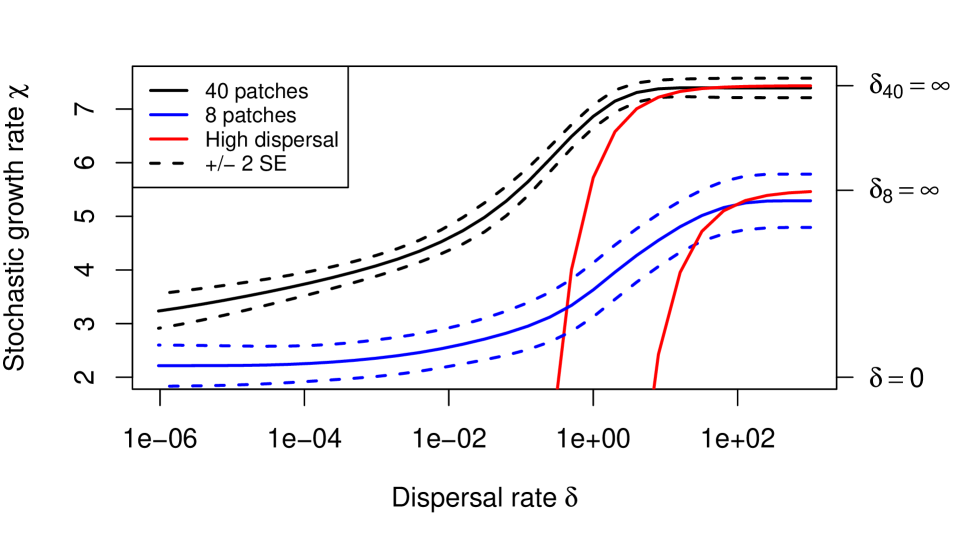
Figure 2. The effect of dispersal rate $\delta$ on populations emigrating more rapidly out of lower quality patches than higher quality patches. Shown is the stochastic growth rate $\chi$ estimated from simulation of the SDE for 100 time units, across a range of values of $\delta$, for both a 40-patch and a 8-patch model. Standard errors are estimated using the standard deviation of the stochastic growth rates across nonoverlapping time segments of a given simulation. Details of the dispersal matrix and parameter values are described in the main text. The right-hand axis shows asymptotic values for $\delta=0$ and $\delta=\infty$, which are: $\chi(0)=\max_{i}\mu_{i}$ and $\chi(\infty)=\mu^{T}\pi-\frac{1}{2}\pi^{T}\Sigma\pi$ (Proposition 4.1). “High dispersal” shows the approximation of the form $\chi(\delta)\approx a+b/\delta$ for large $\delta$ calculated from formula (19) of Theorem 2.

First, we consider the case in which emigration is “adaptive” in the sense that individuals emigrate more rapidly out of lower quality patches than higher quality patches:

$$D_{ij}=\left\{\begin{array}[]{cc}\delta,&\mbox{for }i=1,\dots,n/4\mbox{ and }i\neq j,\\ 10\,\delta,&\mbox{for }i=n/4+1,\dots,n\mbox{ and }i\neq j.\end{array}\right.$$

Here, the parameter $\delta>0$ scales the emigration rate, so that doubling $\delta$ doubles the emigration rate from all patches. As expected, since in this case dispersal is “adaptive”, Figure 2 shows that stochastic growth rate $\chi=\chi(\delta)$ as a function of $\delta$ increases with $\delta$. Moreover, Figure 2 shows asymptotic values at $\delta=\infty$ for each case, and illustrates that the analytic approximation developed later in Theorem 5.2 works reasonably well for large values of $\delta$. The Figure also shows extremely slow convergence as $\delta\to 0$ to $\chi(0)=\max_{i}\mu_{i}-(1/2)\sigma_{i}^{2}$ (note the logarithmic scale on the horizontal axis), indicating that although $\chi$ is continuous at $\delta=0$ by Proposition 5.1 below, it may not be differentiable there.

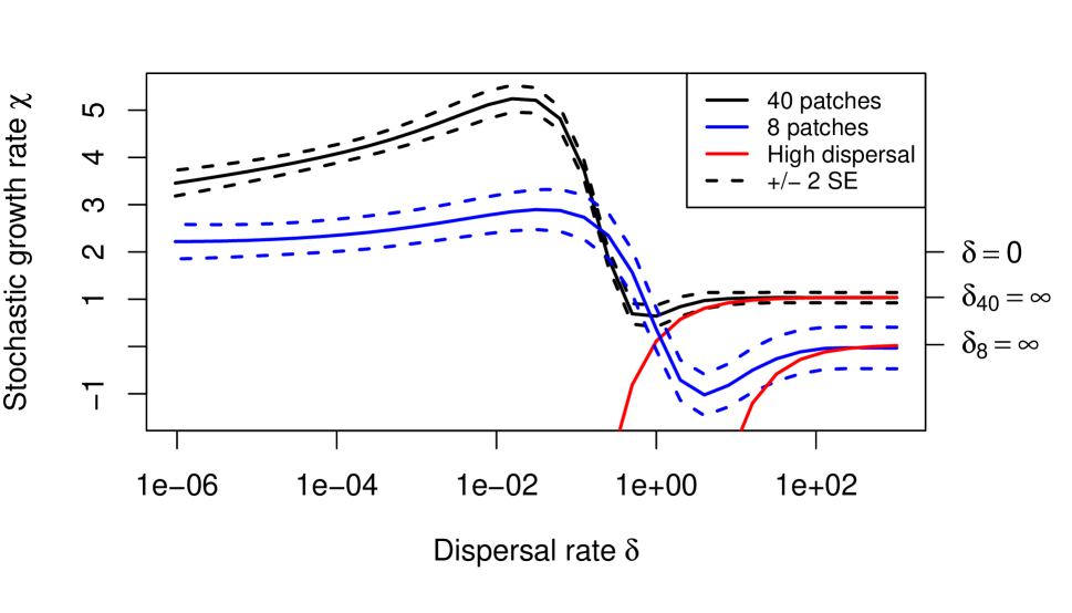
Figure 3. The effect of dispersal rate $\delta$ on populations emigrating more rapidly out of higher quality patches than lower quality patches. Details are as in Figure 2, but with different dispersal scheme; parameter values are described in the main text.

Next we consider a case in which emigration is “maladaptive”, in the sense that individuals emigrate more rapidly out of higher quality patches than out of lower quality patches:

$$D_{ij}=\left\{\begin{array}[]{cc}10\,\delta,&\mbox{for }i=1,\dots,n/4\mbox{ and }i\neq j,\\ \delta,&\mbox{for }i=n/4+1,\dots,n\mbox{ and }i\neq j.\end{array}\right.$$

It is possible to show using the results of Section 5 below that in this regime, high dispersal rates lead to a lower stochastic growth rate than sedentary populations (that is, $\lim_{\delta\to\infty}\chi(\delta)$ is dominated by $\lim_{\delta\to 0}\chi(\delta)$), and yet $\chi(\delta)$ increases with $\delta$ when $\delta$ is large. As illustrated in Figure 3, the stochastic growth rate $\chi(\delta)$ exhibits a rather complex dependence on $\delta$: increasing at low dispersal rates, declining at higher dispersal rates, and finally increasing again at the highest dispersal rates.

In a conservation framework, increasing $\delta$ corresponds to facilitating movement between patches by increasing the size or number of dispersal corridors between patches.

Biological interpretation of Example 3.2. For populations exhibiting adaptive movement, increasing the size or number of dispersal corridors between patches enhances metapopulation growth rates. For populations exhibiting maladaptive movement, however, increasing dispersal rates can either increase or decrease metapopulation growth rates.

4. Ideal free dispersal in a stochastic environment

A basic quandary in evolutionary ecology is, “For a given set of environmental conditions, what dispersal pattern maximizes fitness?” Since fitness in our context corresponds to the stochastic growth rate of the population, we can rephrase this question as, “Given $\mu$ and $\Sigma$, what form of the dispersal matrix $D$ maximizes $\chi$?” Following Fretwell and Lucas [1970], we call such an optimal dispersal mechanism ideal free dispersal as individuals have no constraints on their dispersal (i.e. are “free”) and have complete knowledge about the distribution of spatial-temporal fluctuations (i.e. are “ideal”).

Equation (5) provides a means to answer this question. Because $\Sigma$ has full rank, the function $y\mapsto\frac{1}{2}y^{T}\Sigma y$ is strictly convex, and so Jensen’s inequality implies that

$$\mathbb{E}[\mathbf{Y}_{\infty}^{T}\Sigma\mathbf{Y}_{\infty}]\geq\mathbb{E}[\mathbf{Y}_{\infty}]^{T}\Sigma\,\mathbb{E}[\mathbf{Y}_{\infty}],$$

with equality if and only if the random vector $\mathbf{Y}_{\infty}$ is almost surely constant. Hence, to maximize the stochastic growth rate $\chi$, we need to eliminate the variability in $\mathbf{Y}_{\infty}$, so that $\mathbf{Y}_{\infty}=y$ almost surely for a constant $y$ that is chosen to maximize

(11) $$\mu^{T}y-\frac{1}{2}y^{T}\Sigma\,y$$

subject to the constraint $y\in\Delta$. Under our standing non-degeneracy assumptions on $D$ and $\Sigma$, the law of $\mathbf{Y}_{\infty}$ is supported on all of $\Delta$, and so we cannot actually achieve a situation in which $\mathbf{Y}_{\infty}$ is a constant. However, the following result, which we prove in Appendix B, shows that we can approach this regime arbitrarily closely. Recall that the stationary distribution $\pi$ for an irreducible dispersal matrix $Q$ is a probability vector $\pi\in\Delta$ such that $\pi^{T}Q=0$. We note that any vector $\pi$ in the interior of $\Delta$ is the stationary distribution for some irreducible dispersal matrix $Q$. For example, given $\pi$, we can define $Q=\mathbf{1}\pi^{T}-I$ where $I$ denotes the identity matrix.

Proposition 4.1.

Consider a vector $\pi$ in the interior of $\Delta$ and an irreducible dispersal matrix $Q$ that has $\pi$ as its unique stationary distribution. Let $\mathbf{Y}_{\infty}(\delta)$ be the equilibrium patch distribution and $\chi(\delta)$ be the stochastic growth rate for (3) with $D=\delta Q$. Then $\mathbf{Y}_{\infty}(\delta)$ converges in law to the constant vector $\pi$ as $\delta\to\infty$, and $\chi(\delta)$ converges to $\mu^{T}\pi-\frac{1}{2}\pi^{T}\Sigma\,\pi$ as $\delta\to\infty$.

In the absence of population growth due to deterministic or stochastic effects, each of the dispersal matrices $\delta Q$ in Proposition 4.1 sends the patch distribution to the vector $\pi$ regardless of the initial conditions, and the speed at which this happens increases with $\delta$, so that it becomes effectively instantaneous for large $\delta$. Proposition 4.1 says that this push towards a deterministic equilibrium overcomes any disruptive effects introduced by population growth provided $\delta$ is sufficiently large, and so it is possible to produce random equilibrium patch distributions that are arbitrarily close to any given vector $\pi$ in the interior of $\Delta$. If we further approximate vectors $\pi$ on the boundary of $\Delta$ by ones in the interior, we see that it is possible to produce equilibrium patch distributions that are arbitrarily close to any given vector in $\Delta$.

Given that any patch distribution can be approximated arbitrary closely by the equilibrium patch distribution of a suitable population of rapidly dispersing individuals, the problem of optimizing $\chi$ reduces, as we have already noted, to maximizing the strictly concave function $g(y)=\mu^{T}y-\frac{1}{2}y^{T}\Sigma\,y$ over the compact, convex set $\Delta$. This concavity implies there exists at most one local maximum. Denote this unique maximizer by $y^{*}=(y_{1}^{*},\dots,y_{n}^{*})^{T}$.

It is optimal for all individuals to remain in the single patch $k$ (that is, $y_{k}^{*}=1$) only if

$$\frac{\partial g}{\partial y_{i}}(e_{k})-\frac{\partial g}{\partial y_{k}}(e_{k})=\mu_{i}-\sigma_{ik}-\mu_{k}+\sigma_{kk}<0\text{ for all }i\neq k,$$

where $e_{k}$ is the $k$-th element of the standard basis of $\mathbb{R}^{n}$, or, equivalently,

(12) $$\mu_{k}-\mu_{i}>\sigma_{kk}-\sigma_{ik}\mbox{ for all }i\neq k.$$

Biological interpretation of equation (12). If the variances of environmental fluctuations are sufficiently large in all patches and the spatial covariances in these environmental fluctuations are sufficiently small, then ideal free dispersers occupy multiple patches.

When it is optimal to disperse between several patches, we can solve for the optimal dispersal strategy $y^{*}$ by using the method of Lagrange multipliers. Without loss of generality, assume that the optimal strategy $y^{*}$ makes use of all patches, that is, that $y^{*}$ is in the interior of $\Delta$. Indeed, if the optimal strategy does not make use of all patches, then we can consider analogous problems on the faces of the convex polytope $\Delta$ of the form $\{y\in\Delta:y_{i}=0,\,i\in A\}$, where $A$ is a subset of $\{1,\ldots,n\}$. Because

$$\nabla g(y)=\mu-\Sigma y\mbox{ and }\nabla\left(\sum_{i}y_{i}\right)=\mathbf{1},$$

the optimal $y^{*}$ must satisfy

(13) $$\mu-\Sigma y^{*}=\lambda\mathbf{1},$$

where $\lambda$ is a Lagrange multiplier. Notice that

$$(\Sigma y)_{i}=\frac{1}{\Delta t}\mathbb{E}\left[(E_{t+\Delta t}^{i}-E_{t}^{i})\sum_{j}y_{j}(E_{t+\Delta t}^{j}-E_{t}^{j})\right].$$

Hence, we get the following interpretation.

Biological interpretation of equation (13). Ideal free populations using multiple patches are distributed across the patches in such a way that the differences between the mean per-capita growth rates and the covariances between the within patch noise and the noise experienced on average by an individual are equal in all occupied patches. In particular, the local stochastic growth rates $\mu_{i}-\sigma_{ii}/2$ need not be equal in all occupied patches.

Now,

(14) $$y^{*}=\Sigma^{-1}(\mu-\lambda\mathbf{1}),$$

and the constraint $\mathbf{1}^{T}y=1$ yields

$$1=\mathbf{1}^{T}\Sigma^{-1}(\mu-\lambda\mathbf{1}),\\$$

so that

(15) $$\lambda=\frac{\mathbf{1}^{T}\Sigma^{-1}\mu-1}{\mathbf{1}^{T}\Sigma^{-1}\mathbf{1}}$$

and

(16) $$y^{*}=\Sigma^{-1}\left(\mu-\frac{\mathbf{1}^{T}\Sigma^{-1}\mu-1}{\mathbf{1}^{T}\Sigma^{-1}\mathbf{1}}\mathbf{1}\right).$$

The right-hand side of equation (16) is the optimal vector $y^{*}$ we seek, provided that it belongs to the interior of $\Delta$. Otherwise, as we remarked above, we need to perform similar analyses on the faces of the simplex $\Delta$.

To illustrate the utility of this formula, we examine two special cases: when the environmental noise between patches is uncorrelated, and when the patches experience the same individual levels of noise but they are spatially correlated.

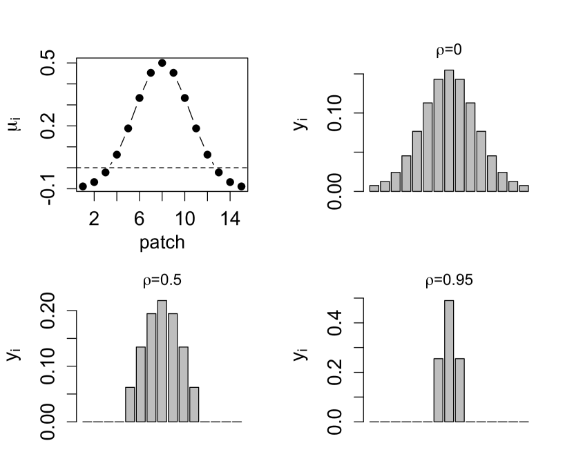
Figure 4. Effects of spatial correlations on the ideal free patch distribution in a 15 patch environment. Per-capita growth rates $\mu_{i}$ are plotted in the top left. The ideal free patch distribution $y^{*}$ is plotted at three levels of spatial correlation $\rho$. Covariances are $\sigma_{ii}=2$ and $\sigma_{ij}=2\rho$ for $i\neq j$.

Example 4.1 Spatially uncorrelated environments.

Suppose that there are no spatial correlations in the environmental noise, so that $\Sigma$ is a diagonal matrix with diagonal entries $\sigma_{ii}=\sigma_{i}^{2}$. It follows from equation (16) that the ideal free patch distribution is

(17) $$y_{i}^{*}=\frac{1}{\sigma_{i}^{2}\sum_{j}1/\sigma_{j}^{2}}\left[\sum_{j}\frac{\mu_{i}-\mu_{j}}{\sigma_{j}^{2}}+1\right],$$

provided that $\sum_{j}(\mu_{j}-\mu_{i})/\sigma_{j}^{2}<1$ for all $i$.

Biological interpretation of equation (17). In the absence of spatial correlations in environmental fluctuations, ideal free dispersers visit all patches whenever the environmental variation is sufficiently great relative to differences in the mean per-capita growth rates. In particular, if all mean per-capita growth rates are equal, then the fraction of individuals in a patch is inversely proportional to the variation in temporal fluctuations in the patch; that is, $y_{i}^{*}=(1/\sigma_{i}^{2})/(\sum_{j}1/\sigma_{j}^{2})$.

Example 4.2 Spatially correlated environments.

Suppose that the infinitesimal variance of the temporal fluctuations in each patch is $\sigma^{2}$ and that the correlation between the fluctuations in any pair of patches is $\rho$. Thus, $\Sigma=\sigma^{2}(1-\rho)I+\sigma^{2}\rho J$, where $J=\mathbf{1}\mathbf{1}^{T}$ is the matrix in which every entry is $1$. Provided that $-\frac{1}{n-1}<\rho<1$, the matrix $\Sigma$ is non-singular with inverse

$$\Sigma^{-1}=\frac{1}{(1-\rho)\sigma^{2}}I-\frac{\rho}{(1-\rho)(1+(n-1)\rho)\sigma^{2}}J.$$

Denoting by $\bar{\mu}=\frac{1}{n}\sum_{i}\mu_{i}$ the average across the patches of the mean per-capita growth rates, the optimal dispersal strategy is given by

(18) $$y_{i}^{*}=\frac{\mu_{i}-\bar{\mu}}{\sigma^{2}(1-\rho)}+\frac{1}{n}$$

provided that $y^{i}_{*}>0$ for all $i$. Notice that (18) agrees with (17) when $\rho=0$ and $\sigma_{i}=\sigma$.

Biological interpretation of equation (18). If environmental fluctuations have a sufficiently large variance $\sigma^{2}$, then ideal free dispersers visit all patches and spend more time in patches that support higher mean per-capita growth rates. Increasing the common spatial correlation $\rho$ results in ideal free dispersers spending more time in patches whose mean per-capita growth rate is greater than the average of the mean per-capita growth rates and less time in other patches (Fig. 4). When the spatial correlations are sufficiently large, it is no longer optimal to disperse to the patches with lower mean per-capita growth rates ($\rho=0.5$ and $\rho=0.95$ in Fig. 4).

5. The effect of constraints on dispersal

While the ideal free patch distribution is a useful idealization to investigate how organisms should disperse in the absence of constraints, organisms in the natural world have limits on their ability to disperse and to collect and interpret environmental information. Recall from Section 4 that if the optimal patch distribution $y^{*}$ for an ideal free disperser is in the interior of the probability simplex $\Delta$, then, loosely speaking, the ideal free disperser achieves the maximal stochastic growth rate by using a strategy for which dispersal rate matrix is of the form $D=\delta Q$, where $Q$ is any irreducible dispersal matrix with $(y^{*})^{T}Q=0$ and $\delta=\infty$. At the opposite extreme, if $y^{*}$ assigns all of its mass to a single patch, then an ideal free disperser never leaves that single most-favored patch.

To get a better understanding of how constraints on dispersal influence population growth, we consider dispersal matrices of the form $D=\delta Q$, where $\delta\geq 0$ and $Q$ is a fixed irreducible dispersal matrix $Q$ with a stationary distribution $\pi$ that is not necessarily the optimal patch distribution for an ideal free disperser in the given environmental conditions. We write $\chi(\delta)$ for the stochastic growth rate of the population as a function of the dispersal parameter $\delta$ and ask which choice of $\delta$ maximizes $\chi(\delta)$. In particular, we are interested in conditions under which some intermediate $\delta>0$ maximizes the stochastic growth rate $\chi(\delta)$.

We know from Proposition 4.1 that $\chi(\delta)$ approaches $\pi^{T}\mu-\frac{1}{2}\pi^{T}\Sigma\pi$ as $\delta\to\infty$. We therefore set $\chi(\infty)=\pi^{T}\mu-\frac{1}{2}\pi^{T}\Sigma\pi$. On the other hand, if there is no dispersal ($\delta=0$), then $\lim_{t\to\infty}\frac{1}{t}\log X_{t}^{i}=\mu_{i}-\frac{\sigma_{i}^{2}}{2}$ with probability one whenever $X_{0}^{i}>0$, and so $\lim_{t\to\infty}\frac{1}{t}\log S_{t}=\max_{i}\{\mu_{i}-\frac{\sigma_{i}^{2}}{2}\}$ whenever $X_{0}^{i}>0$ for all $i$. Hence, it is reasonable to set $\chi(0)=\max_{i}\{\mu_{i}-\frac{\sigma_{i}^{2}}{2}\}$. The following result, which we prove in Appendix C, implies that the function $\delta\mapsto\chi(\delta)$ is continuous on $[0,\infty)$.

Proposition 5.1.

The function $\delta\mapsto\chi(\delta)$ is analytic on the interval $(0,\infty)$ and continuous at the point $\delta=0$.

One way to establish that $\chi(\delta)$ is maximized for an intermediate value of $\delta$ is to show that $\chi(0)<\chi(\infty)$ and that $\chi(\delta)>\chi(\infty)$ for all sufficiently large $\delta$. The following theorem provides an asymptotic approximation for $\chi(\delta)$ when $\delta$ is large that allows us to check when the latter condition holds. We prove the theorem under the hypothesis that the dispersal matrix $Q$ is reversible with respect to its stationary distribution $\pi$; that is, that $\pi_{i}Q_{ij}=\pi_{j}Q_{ji}$ for all $i,j$. Reversibility implies that at stationarity the Markov chain defined by $Q$ exhibits “balanced dispersal in the absence of local demography.” Namely, if a large number of individuals are independently executing the equilibrium movement dynamics, then the rate at which individuals move from patch $i$ to patch $j$ equals the rate at which individuals move from patch $j$ to patch $i$. We note that diffusive movement (that is, the matrix $Q$ is symmetric) and any form of movement along a one-dimensional landscape (that is, the matrix $Q$ is tridiagonal) are examples of reversible Markov chains. We provide a proof of the theorem in Appendix D. Corollary 5.3 below, which we prove in Appendix E, provides a more readily computable expression for the asymptotics of the stochastic growth rate under further assumptions.

Theorem 5.2.

Suppose that $Q$ is reversible with respect to its stationary distribution $\pi$. Then,

(19) $$\chi({\delta}) = \left(\mu^{T}\pi-\frac{1}{2}\pi^{T}\Sigma\pi\right)+\frac{1}{\delta}\biggl{[}(\mu-\Sigma\pi)^{T}\nu$$

$$\qquad-\frac{1}{2}\int_{0}^{\infty}\mathrm{Tr}\left(\exp(Q^{T}s)\left(\mathrm{diag}(\pi)-\pi\pi^{T}\right)\Sigma\left(\mathrm{diag}(\pi)-\pi\pi^{T}\right)\exp(Qs)\Sigma\right)\,ds\biggr{]}+\mathrm{O}(\delta^{-\frac{5}{4}})$$

as $\delta\to\infty$, where $\nu$ is the unique vector satisfying $\mathbf{1}^{T}\nu=0$ and $Q^{T}\nu=-\left(\mathrm{diag}(\pi)-\pi\pi^{T}\right)(\mu-\Sigma\pi)$.

When the dispersal matrix $D=\delta Q$ is consistent with ideal dispersal in the limit $\delta\to\infty$, equation (13) implies that $(\mu-\Sigma\pi)^{T}\nu=\lambda\mathbf{1}^{T}\nu=0$. On the other hand, the proof of Theorem 5.2 shows that

$$\int_{0}^{\infty}\mathrm{Tr}\left(\exp(Q^{T}s)\left(\mathrm{diag}(\pi)-\pi\pi^{T}\right)\Sigma\left(\mathrm{diag}(\pi)-\pi\pi^{T}\right)\exp(Qs)\Sigma\right)\,ds=\mathrm{Tr}\left(\mathbb{E}[\mathbf{V}_{\infty}\mathbf{V}_{\infty}^{T}]\Sigma\right)>0$$

where $\mathbf{V}_{\infty}$ is a Gaussian random vector. Hence, as expected, $\chi(\delta)$ is an increasing function for large $\delta$ when $\pi$ corresponds to the ideal free distribution associated with $\mu$ and $\Sigma$. However, when $\pi$ does not correspond to the ideal free distribution, $\chi(\delta)$ may be increasing or decreasing for large $\delta$ as we illustrate below.

When $Q$ and $\Sigma$ commute, the asymptotic expression (19) for $\chi(\delta)$ simplifies a great deal.

Corollary 5.3.

Suppose that $Q$ is symmetric and $Q\Sigma=\Sigma Q$. Let $\lambda_{1}\leq\ldots\leq\lambda_{n-1}<\lambda_{n}=0$ be the eigenvalues of $Q$ with corresponding orthonormal eigenvectors $\xi_{1},\ldots,\xi_{n}$. Then, the eigenvalues $\theta_{1},\ldots,\theta_{n}$ of $\Sigma$ can be ordered so that $\Sigma\xi_{k}=\theta_{k}\xi_{k}$, for each $1\leq k\leq n$, and the approximation (19) reduces to

(20) $$\chi(\delta)=\left(\bar{\mu}-\frac{1}{2n}\theta_{n}\right)-\frac{1}{\delta n}\left[\sum_{k=1}^{n-1}\frac{1}{\lambda_{k}}\left((\xi_{k}^{T}\mu)^{2}-\frac{1}{4n}\theta_{k}^{2}\right)\right]+\mathrm{O}(\delta^{-5/4})$$

as $\delta\to\infty$, where $\bar{\mu}=\frac{1}{n}\sum\mu_{i}$.

To illustrate the utility of this latter approximation, we develop more explicit formulas for three scenarios: diffusive movement in a landscape where all patches are equally connected (that is, a classic “Levins” style landscape [Levins, 1969]), diffusive movement in a landscape consisting of a ring of patches, and diffusive movement in a landscape with multiple spatial scales (that is, a hierarchical Levins landscape).

Example 5.1 Fully connected metapopulations with unbiased movement.

Consider a population in which individuals disperse at the same per-capita rate $\delta/n$ between all pairs of patches. Let $\sigma^{2}$ be the variance of the within patch fluctuations and $\rho$ be the correlation in these fluctuations between any pair of patches. Under these assumptions, the dispersal matrix is $Q=J/n-I$ and the environmental covariance matrix is $\Sigma=(1-\rho)\sigma^{2}I+\rho\sigma^{2}J$, where recall that $J=\mathbf{1}\mathbf{1}^{T}$ is the matrix of all ones. Because $Q$ is symmetric, the stationary distribution of $Q$ is uniform; that is, $\pi_{1}=\dots=\pi_{n}=\frac{1}{n}$. Hence, in the absence of population growth there would be equal numbers of individuals in each patch at large times.

Because the matrices $I$ and $J$ commute, the matrices $Q$ and $\Sigma$ also commute. Recall the notation of Corollary 5.3. The eigenvector $\xi_{n}$ is $\frac{1}{\sqrt{n}}\mathbf{1}$. If $\xi$ is any vector of length one orthogonal to $\xi_{n}$, then $J\xi=0$, and so $Q\xi=-\xi$ and $\Sigma\xi=(1-\rho)\sigma^{2}\xi$. We may thus take $\xi_{1},\ldots,\xi_{n-1}$ to be any orthonormal set of vectors orthogonal to $\xi_{n}$. Moreover, $\lambda_{1}=\cdots=\lambda_{n-1}=-1$ and $\theta_{1}=\cdots=\theta_{n-1}=(1-\rho)\sigma^{2}$.

Now, $(\xi_{n}^{T}\mu)^{2}=(1/n)\left(\sum_{k=1}^{n}\mu_{k}\right)^{2}=n(\bar{\mu})^{2}$, and so Parseval’s identity implies that $\sum_{k=1}^{n-1}(\xi_{k}^{T}\mu)^{2}=\sum_{k=1}^{n}\mu_{k}^{2}-n(\bar{\mu})^{2}=\mu^{T}\mu-n(\bar{\mu})^{2}$. Denote the variance of the vector $\mu$ by

$$\mathrm{Var}[\mu]=\frac{1}{n}\mu^{T}\mu-(\bar{\mu})^{2}=\frac{1}{n}\sum_{k=1}^{n-1}(\xi_{k}^{T}\mu)^{2}.$$

Substituting these observations into equation (20), we get that

(21) $$\chi(\delta)=\bar{\mu}-\frac{\sigma^{2}}{2n}\left(1+(n-1)\rho\right)+\frac{1}{\delta}\left[\mathrm{Var}[\mu]-\frac{(n-1)((1-\rho)\sigma^{2})^{2}}{4n^{2}}\right]+\mathrm{O}(\delta^{-\frac{5}{4}}).$$

Recall that for the special case of two uncorrelated patches with $D_{12}=D_{21}=\delta/2$, $\mu_{1}=\mu_{2}=\mu$, and $\sigma_{1}=\sigma_{2}=\sigma$, we showed from our exact formula for $\chi(\delta)$ in the two patch case that

$$\chi(\delta)\approx\mu-\frac{\sigma^{2}}{4}-\frac{1}{\delta}\frac{\sigma^{4}}{16}$$

as $\delta\to\infty$, see (10). Hence, this approximation agrees with (21).

Approximation (21) implies that $\chi(\delta)$ is decreasing for large $\delta$ whenever

(22) $$\frac{n}{\sqrt{n-1}}\sqrt{\mathrm{Var}[\mu]}>\frac{(1-\rho)\sigma^{2}}{2},$$

and that $\chi(\delta)$ is increasing if the opposite inequality holds. We have remarked that, in general, an intermediate dispersal rate is optimal when $\chi(0)<\chi(\infty)$ and $\chi(\delta)>\chi(\infty)$ for all sufficiently large $\delta$. This will occur for individuals in this diffusive dispersal regime when

(23) $$\frac{(1-\rho)\sigma^{2}}{2}>\frac{\max_{i}\mu_{i}-\bar{\mu}}{1-1/n}$$

and (22) holds. In particular, when there are many patches (that is, $n\to\infty$), inequalities (23) and (22) are both satisfied if

$$(1-\rho)\sigma^{2}/{2}>\max_{i}\mu_{i}-\bar{\mu}>0.$$

Biological interpretation of equations (22) and  (23). Highly diffusive movement has a negative impact on population growth whenever there are sufficiently many patches and there is sufficient spatial variation in the mean per-capita growth rates. Alternatively, if there is no spatial variation in the mean per-capita rates and stochastic fluctuations are not perfectly correlated, then the population growth rate continually increases with higher dispersal rates. This latter observation is consistent with individuals being distributed equally across the landscape is the optimal patch distribution. In contrast, if there is some spatial variation in the mean per-capita growth rates and there are sufficiently large, but not perfectly correlated environmental fluctuations, then an intermediate dispersal rate maximizes the stochastic growth rate for diffusively dispersing populations.

In order to apply Corollary 5.3, we need to to simultaneously diagonalize the matrices $Q$ and $\Sigma$. A situation in which this is possible and the resulting formulas provide insight into biologically relevant scenarios is when the dispersal mechanism and the covariance structure of the noise both exhibit the symmetries of an underlying group. Example 5.1 above is a particular instance of this situation.

More specifically, we suppose that the patches can be labeled with the elements of a finite group $G$ in such a way that the migration rate $Q_{g,h}$ and environmental covariance $\Sigma_{g,h}$ between patches $g$ and $h$ both only depend on the “displacement” $gh^{-1}$ from $g$ to $h$ in $G$. That is, we assume there exist functions $q$ and $s$ on $G$ such that $Q_{gh}=q(gh^{-1})$ and $\Sigma_{gh}=s(gh^{-1})$. For instance, if $G$ is the group of integers modulo $n$, then the habitat has $n$ patches arranged in a circle, and the dispersal rate and environmental covariance between two patches only depends on the distance between them, measured in steps around the circle. We do not require that the vector $\mu$ of mean per-capita growth rates satisfies any symmetry conditions.

The matrices $Q$ and $\Sigma$ will commute if $q$ and $s$ are class functions, that is, if $q(gh)=q(hg)$ and $s(gh)=s(hg)$ for all $g,h\in G$. We assume this condition holds from now on. Note that if $G$ is Abelian (that is, the group operation is commutative), then any function is a class function.

5.1. Background on group representations

We now record a few facts about representation theory, the tool that will enable us to find the eigenvalues and eigenvectors of $Q$ and $\Sigma$, resulting in Theorem 5.4. We refer readers interested in more detail to [Serre, 1977, Diaconis, 1988], while readers interested in less mathematical detail may skip directly to Examples 5.2 and 5.3 without loss of continuity.

A unitary representation of a group $G$ is a homomorphism $\rho$ from $G$ into the group of $d_{\rho}\times d_{\rho}$ unitary matrices, where $d_{\rho}$ is called the degree of the representation. Two representations $\rho^{\prime}$ and $\rho^{\prime\prime}$ are equivalent if there exists a unitary matrix $U$ such that $\rho^{\prime\prime}(g)=U\rho^{\prime}(g)U^{-1}$ for all $g\in G$. A representation $\rho^{\prime}$ is irreducible if it is not equivalent to some representation $\rho^{\prime\prime}$ for which $\rho^{\prime\prime}(g)$ is of the same block diagonal form for all $g\in G$. A finite group has a finite set of inequivalent, irreducible, unitary representations, which we denote by $\hat{G}$. The simplest representation is the trivial representation $\rho_{\mbox{tr}}$ of degree one, for which $\rho_{\mbox{tr}}(g)=1$ for all $g$.

For a simple example that we will return to, let $G=\mathbb{Z}_{n}$, the group of integers modulo $n$. Since $\mathbb{Z}_{n}$ is Abelian, all the irreducible representations are one-dimensional ($d_{\rho}=1$ for all $\rho\in\hat{G}$), and are of the form $\rho^{(m)}(j)=\exp(2\pi imj/n)$, so that $\hat{G}=\{\rho^{(m)}_{m}:0\leq m\leq n-1\}$.

The matrix entries of irreducible representations are orthogonal: for $\rho^{\prime},\rho^{\prime\prime}\in\hat{G}$,

(24) $$\sum_{g\in G}\rho^{\prime}_{ij}(g)\rho^{\prime\prime}_{k\ell}(g)^{*}=\begin{cases}\frac{\#G}{d_{\rho}},&\text{if $\rho^{\prime}=\rho^{\prime\prime}$ and $(i,j)=(k,\ell)$},\\ 0,&\text{otherwise,}\end{cases}$$

where $z^{*}$ denotes the complex conjugate of a complex number $z$, and $\#G$ is the number of elements of $G$.

The Fourier transform of a function $f:G\to\mathbb{C}$ is a function $\hat{f}$ on $\hat{G}$ defined by

(25) $$\hat{f}(\rho):=\sum_{g\in G}f(g)\rho(g)\quad\mbox{for}\;\rho\in\hat{G}.$$

Note that $\hat{f}(\rho)$ is a $d_{\rho}\times d_{\rho}$ matrix. It follows from the orthogonality properties of the matrix entries of the irreducible representations recorded above that the Fourier transform may be inverted, giving $f$ explicitly as the linear combination of matrix entries of $\hat{f}$. The inversion formula is

$$f(g)=\frac{1}{\#G}\sum_{\rho\in\hat{G}}d_{\rho}\mathop{\mbox{Tr}}\left(\rho(g^{-1})\hat{f}(\rho)\right).$$

For $G=\mathbb{Z}_{n}$, this is the familiar discrete Fourier transform, for which orthogonality of matrix entries is the fact that $(1/n)\sum_{j=0}^{n-1}\exp(2\pi ij(\ell-m)/n)=\delta_{\ell m}$. The transform is given by $\hat{f}(\rho^{(m)})=\sum_{k=0}^{n-1}f(k)\exp(2\pi imk/n)$ for $0\leq m\leq n-1$, and $f(k)=(1/n)\sum_{m=0}^{n-1}\hat{f}(\rho^{(m)})\exp(-2\pi imk/n)$. The trivial character is $\kappa_{\mbox{\rm tr}}=\rho^{(0)}$.

Associated with a representation $\rho\in\hat{G}$ is its character $\kappa$, defined by $\kappa(g):=\mathop{\mbox{Tr}}\rho(g)$. We write $\tilde{G}$ for the set of characters of irreducible representations. The characters are class functions, and form an orthogonal basis for the subspace of class functions on $G$ and all have the same norm: $\sum_{g\in G}|\kappa(g)|^{2}=\#G$, where $|z|=\sqrt{zz^{*}}$ is the modulus of the complex number $z$. For $\rho\in\hat{G}$ with character $\kappa\in\tilde{G}$, the Fourier transform of a class function $f$ satisfies

$$\hat{f}(\rho)=\frac{1}{d_{\rho}}\tilde{f}(\kappa)I$$

where $I$ is the $d_{\rho}\times d_{\rho}$ identity matrix and

(26) $$\tilde{f}(\kappa):=\sum_{g\in G}f(g)\kappa(g).$$

Consequently,

(27) $$f(g)=\frac{1}{\#G}\sum_{\kappa\in\tilde{G}}\kappa(g)^{*}\tilde{f}(\kappa).$$

As noted above, if $G=\mathbb{Z}_{n}$ then all irreducible representations are one-dimensional, so in this case we may identify the characters with the irreducible representations, $\hat{G}=\tilde{G}$. Since $\mathbb{Z}_{n}$ is Abelian, all functions on $\mathbb{Z}_{n}$ are class functions, so that the two Fourier transforms (25) and (26) are equal.

Finally, given a function $f$ on $G$ and character $\kappa$, define

$$\|f\|_{\kappa}^{2}:=\frac{d_{\rho}}{\#G}\sum_{g,h\in G}\kappa(gh^{-1})f(g)f(h)^{*}.$$

The following theorem is proved in Appendix F.

Theorem 5.4.

Suppose that the $n$ patches are labeled by a finite group $G$ in such a way that $Q_{gh}=q(gh^{-1})$ and $\Sigma_{gh}=s(gh^{-1})$, where $q$ and $s$ are class functions. Suppose further that $q(g)=q(g^{-1})$, $g\in G$, so that the matrix $Q$ is symmetric. Let $\bar{\mu}=\frac{1}{\#G}\sum_{g\in G}\mu(g)$ and $\bar{s}=\frac{1}{\#G}\sum_{g\in G}s(g)$. Then,

(28) $$\chi(\delta)=\left(\bar{\mu}-\frac{1}{2}\bar{s}\right)-\frac{1}{\delta n}\sum_{\kappa\in\tilde{G}\setminus\{\kappa_{\mbox{\rm tr}}\}}\frac{d_{\kappa}}{\tilde{q}(\kappa)}\left(\|\mu\|_{\kappa}^{2}-\frac{1}{4n}\tilde{s}(\kappa)^{2}\right)+O(\delta^{-5/4})$$

as $\delta\to\infty$. Furthermore, $\tilde{q}(\kappa)<0$ for all $\kappa\in\tilde{G}\setminus\{\kappa_{\mbox{\rm tr}}\}$.

Roughly speaking, this expression tells us about the respective roles of variance of patch quality ($\mu$) and covariance of environmental noise ($s$). The fact that $\tilde{q}(\kappa)$ is negative for all $\kappa$ leads to the following.

Biological interpretation of equation (28). If variability in patch quality at a certain scale is larger than the correlation in environmental noise at that scale, in a sense made precise above, then the stochastic growth rate decreases with increasing dispersal rates at that scale. Conversely, if environmental noise is strongly correlated between patches and the mean patch quality is similar, then more dispersal is expected to be better. The relevant sense of “at that scale” is in the sense of the Fourier transform, analogous to the “frequency domain” in Fourier analysis.

Example 5.2 Circle of Patches.

Suppose that the $n$ patches of a habitat are arranged in a circle and are labeled by $\mathbb{Z}_{n}=\{0,1,\ldots,n-1\}$, the group of integers modulo $n$ with identity element $0$. As reviewed above, the Fourier transform is the familiar discrete Fourier transform.

If we assume that individuals disperse only to neighboring patches and these dispersal rates are equal, then $q(1)=q(n-1)=1/2$, $q(0)=-1$ and $q(2)=\ldots=q(n-2)=0$. Assume the environmental noise is independent between patches and has variance $\sigma^{2}$ i.e. $s(0)=\sigma^{2}$ and $0=s(1)=\ldots=s(n-1)$. Finally, suppose that patch quality as measured by the average per-capita growth rates is spatially periodic, so that $\mu(k)=\bar{\mu}+c\;\cos(2\pi k\ell/n)$ for some $c>0$, $\bar{\mu}$, and $1\leq\ell<n/2$.

Under this set of assumptions, we can compute that for $m\neq 0$, $\tilde{q}(m)=\cos(2\pi m/n)-1$ and $\tilde{s}(m)=\sigma^{2}$. Furthermore, $\|\mu\|^{2}_{\kappa_{\ell}}=\|\mu\|^{2}_{\kappa_{n-\ell}}=nc^{2}/4$ and $\|\mu\|^{2}_{\kappa_{m}}=0$ otherwise. From these computations, Theorem 5.4 implies that

$$\chi(\delta)\approx\bar{\mu}-\sigma^{2}/2-\frac{1}{\delta n}\left(\frac{nc^{2}}{2(\cos(2\pi\ell/n)-1)}-\sum_{m=1}^{n-1}\frac{\sigma^{2}}{4n(\cos(2\pi m/n)-1)}\right)$$

for large $\delta$. Using the identity $\sum_{k=1}^{n-1}(1-\cos(2\pi k/n))^{-1}=(n^{2}-1)/6$ (see equation 1.381.1 in Gradshteyn and Ryzhik [2007]’s table of integrals and series), this approximation simplifies to

(29) $$\chi(\delta)\approx\bar{\mu}-\sigma^{2}/2+\frac{1}{4\delta n^{2}}\left(\frac{2n^{2}c^{2}}{1-\cos(2\pi\ell/n)}-\frac{1}{6}(n^{2}-1)\sigma^{4}\right).$$

Since $\chi(0)=\bar{\mu}+c-\sigma^{2}/2$, high dispersal is better than no dispersal if $\chi(\infty)-\chi(0)=\sigma^{2}(1-1/n)/2-c>0$. When the number of patches is sufficiently large, this inequality implies that highly dispersive populations grow faster than sedentary populations provided that the temporal variation is sufficiently greater than the spatial variation in per-capita growth rates i.e. $\sigma^{2}>2c$. On the other hand, $\chi(\delta)$ is decreasing for large $\delta$ if the coefficient of $1/\delta$ is positive i.e.

$$4c^{2}>\frac{1}{3}(1-\cos(2\pi\ell/n))(1-n^{-2})\sigma^{4}.$$

Hence, if $\ell/n$ is small enough, then $\chi(\delta)$ is decreasing for large $\delta$.

Biological interpretation of equation (29). In a circular habitat with nearest-neighbor dispersal and sinusoidally varying patch quality, intermediate dispersal rates maximize the stochastic growth rate provided that spatial heterogeneity occurs on a short scale (i.e. $\ell/n$ sufficiently small) and temporal variability is sufficiently large.

Example 5.3 Multi-scale patches.

Suppose now that our organism lives in a hierarchically structured habitat. For example, individuals might live on bushes, the bushes grow around the edges of clearings, and the clearings are scattered across an archipelago of islands. We label each bush with an ordered triple recording on which island, in which clearing, and in what bush around the clearing it lives, so that for instance $(2,1,4)$ denotes the fourth bush in the first clearing of the second island. To make the mathematical picture a pretty one, we suppose that each of the $I$ islands has the same number $C$ of clearings and each clearing has the same number $B$ of bushes. This enables us identify the habitat structure with the group $\mathbb{Z}_{I}\otimes\mathbb{Z}_{C}\otimes\mathbb{Z}_{B}$, where, as above, $\mathbb{Z}_{m}$ is the group of integers modulo $m$. We will get particularly simple and interpretable results if we also assume that dispersal rates and environmental covariances only depend on the scale at which the movement occurs – between bushes, clearings, or islands.

Although it requires imaginative work to find examples with many more scales than this (do the organism’s fleas have fleas?) it does not cost us anything to work in greater generality. Suppose, then, that the patches in the habitat are labeled with the group $G=G_{1}\otimes\cdots\otimes G_{k}$, where $G_{j}=\mathbb{Z}_{n_{j}}$ for $1\leq j\leq k$.

Thus, one patch is labeled with the identity element $\mathbf{id}_{G}=(\mathbf{id}_{1},\ldots,\mathbf{id}_{k})$ and every other patch is labeled by the displacement required to get there from $\mathbf{id}_{G}$. The later coordinates are understood to be at finer “scales”, so that if $g_{i}=h_{i}$ for all $1\leq i\leq j-1$, then $g$ and $h$ represent patches in the same metapatch at scale $j$. For instance, in our example above, the archipelago of islands is the single metapatch at scale $1$ and the metapatches at scales $2$ and $3$ are, respectively, the islands and the clearings. We label the metapatches at scale $r$ with the set $Z_{r}:=\{g\in G:g_{r}=\mathbf{id}_{r},\ldots g_{k}=\mathbf{id}_{k}\}$, with the convention that $Z_{k+1}:=G$. Because a label $g=(g_{1},\ldots,g_{k})\in G$ represents displacement, the coordinate of the leftmost non-identity element of $g$, denoted by

$$\ell(g):=\min\{j:g_{j}\neq\mathbf{id}_{j}\}\mbox{ and }\ell(\mathbf{id}_{G})=k+1,$$

tells us the scale on which the motion occurs: $g\in G$ corresponds to a displacement that moves between patches within the same metapatch at scale $\ell(g)$ but moves from a patch within a metapatch at scale $\ell(g)+1$ to a patch within some other metapatch at that scale. Note that $1\leq\ell(g)\leq k+1$.

We assume that the dispersal rate and the environmental covariance between two patches only depends on the scale of the displacement necessary to move between the two patches. That is, we suppose there are numbers $q_{1},\ldots,q_{k+1}$ and $s_{1},\ldots,s_{k+1}$ such that $q(g)=q_{\ell(g)}$ and $s(g)=s_{\ell(g)}$.

In Appendix G we show that the Fourier transforms appearing in Theorem 5.4 depend on the following quantities. Let $N_{r}:=\#Z_{r}=\prod_{j=1}^{r-1}n_{j}$ be the number of metapatches at scale $r$. Write $\bar{Z}_{r}:=\{g\in G:g_{j}=\mathbf{id}_{j},\;j\leq r\}$ for the subgroup of displacements that move from one patch to another within the same metapatch at scale $r+1$ and set $\bar{N}_{r}:=\#\bar{Z}_{r}=\prod_{j={r+1}}^{k}n_{j}$. Set

$$v_{\mu}(r):=\frac{1}{N_{r}}\sum_{g\in Z_{r}}\left(\frac{1}{n_{r}}\sum_{h\in G_{r}}\left(\frac{1}{\bar{N}_{r}}\sum_{z\in\bar{Z}_{r}}\mu(ghz)\right)^{2}-\left(\frac{1}{n_{r}}\sum_{h\in G_{r}}\frac{1}{\bar{N}_{r}}\sum_{z\in\bar{Z}_{r}}\mu(ghz)\right)^{2}\right).$$

We can interpret this quantity as follows. There are $N_{r}$ metapatches at scale $r$. Each one has within it $n_{r}$ metapatches at scale $r+1$. First, compute the average of $\mu$ over all the patches within each metapatch at scale $r+1$, then compute the variance of these averages within each metapatch at scale $r$, and finally average these variances across all the metapatches at scale $r$ to produce $v_{\mu}(r)$. Thus, $v_{\mu}(r)$ measures the variability in $\mu$ that can be attributed to scale $r+1$. Set

$$\tilde{s}(r)=\sum_{\ell=r}^{k}(s_{\ell+1}-s_{\ell})\bar{N}_{\ell}$$

and

$$\tilde{q}(r)=-\sum_{\ell=1}^{r}q_{\ell}(\bar{N}_{\ell-1}-\bar{N}_{\ell})-q_{r}\bar{N}_{r}.\\$$

The following result agrees with equation (21), which describes the special case where there is a single scale.

Theorem 5.5.

For a habitat with the above multi-scale structure, equation (19) reduces to

(30) $$\chi(\delta)=\left(\bar{\mu}-\frac{1}{2}\bar{s}\right)-\frac{1}{\delta}\sum_{r=1}^{k}\frac{1}{\tilde{q}(r)}\left(v_{\mu}(r)-\frac{N_{r+1}-N_{r}}{4N_{k+1}^{2}}\tilde{s}(r)^{2}\right)+O(\delta^{-5/4})$$

as $\delta\to\infty$. Furthermore, $\tilde{q}(r)<0$ for all $1\leq r\leq k$.

Note that if $s_{\ell}$ increases with $\ell$ (that is, two patches within the same metapatch have a higher environmental covariance than two patches in different metapatches at that scale), then $\tilde{s}(r)$ decreases with $r$. Also, if $q_{\ell}$ increases with $\ell$ (that is, there is a higher rate for dispersing to a patch within the same metapatch at some scale than to a patch in another metapatch at that scale), then $\tilde{q}(r)$ is negative and decreases with $r$. Using these observations, we may read off several things from (30).

First, consider a simple example with a fixed, large number $n$ of patches distributed among a variable number of islands. Now $k=2$, and let the number of islands $n_{1}=1/\alpha$, with $\alpha\geq 1$, so that the number of patches on each island is $n_{2}=\alpha n$. In this case, $N_{1}=1$, $N_{2}=1/\alpha$, and $N_{3}=n$, while $\bar{N}_{0}=n$, $\bar{N}_{1}=\alpha n$, and $\bar{N}_{2}=1$, so (30) reads

$$\chi(\delta) \approx (\bar{\mu}-\frac{1}{2}\bar{s})-\frac{1}{\delta}\left\{-\frac{v_{\mu}(1)}{q_{1}n}+\frac{(1-\alpha)((s_{3}-s_{2})+\alpha n(s_{2}-s_{1}))^{2}}{\alpha q_{1}n^{2}}-\frac{v_{\mu}(2)-(\alpha n-1)(s_{3}-s_{2})^{2}}{\alpha n^{2}(q_{2}\alpha+q_{1}(1-\alpha))}\right\}$$

$$= (\bar{\mu}-\frac{1}{2}\bar{s})-\frac{\alpha(1-\alpha)(s_{2}-s_{1})^{2}}{\delta q_{1}}+O(n^{-1}).$$

The effect of higher dispersal depends on the difference in covariances between patches on the same island and on different islands, and on the number of islands.

Biological interpretation of equation (5.3). If a sufficiently large number of patches are distributed equally across a number of islands, then for a given dispersal pattern, the stochastic growth rate increases with the dispersal rate (at high levels of dispersal). This effect is strongest if there are only two islands (i.e. $\alpha=1/2$).

Secondly, imagine a fixed ensemble of patches with varying mean per-capita growth rates and consider the following two possibilities for assignment of these patches to metapatches at scale $2$ (the islands in our bush-clearing-island example). One possibility is that some islands are assigned patches that are primarily of high quality, whereas other islands are mostly assigned poor patches. The other possibility is that patches of different quality are evenly spread across the islands, with the range of quality within an island similar to the range of quality between islands. In the first case, the variance across islands of within-island means is comparable to the variance across all patches, so $v_{\mu}(1)\approx v_{\mu}(k)$. In the second case, the within-island means are approximately constant, so that $v_{\mu}(1)$ will be small. Therefore, since $\tilde{q}(r)$ is negative for all $r$, having local positive association of $\mu$ at nearby patches leads to higher stochastic growth rates, at least for large enough values of the dispersal parameter $\delta$.

Biological interpretation of equation (30). All other things being equal, the species will do better if the good habitat is concentrated on particular islands, rather than spread out across many.

Finally, we can observe that adding new scales of metapatch may change the situation from one in which $\chi(\delta)$ is maximal at high values of the dispersal parameter $\delta$ to one in which $\chi(\delta)$ is maximal at intermediate values of $\delta$, or vice-versa. If $n_{1}=1$, then $\tilde{s}(1)$ and $v_{\mu}(1)$ are both zero, and changing $n_{1}$ (for example, going from one to several islands in our example) will increase $\tilde{s}(1)$. Changing $n_{1}$ will also add the quantity $-q_{1}(n_{1}-1)\bar{N}_{1}$ to all values of $\tilde{q}(r)$. The result of this could be to change the sign of the coefficient of $\frac{1}{\delta}$ in (19).

Biological interpretation of equation (30). The optimal level of dispersal for a subpopulation, and the growth rate at that level of dispersal, may differ drastically depending on whether it is connected (or connectable) by dispersal to other subpopulations.

6. Discussion

Classical ecology theory predicts that environmental stochasticity increases extinction risk by reducing the long term per-capita growth rate of populations [May, 1975, Turelli, 1978]. For sedentary populations in a spatially homogeneous yet temporally variable environment, a simple model of their growth is given by the stochastic differential equation $dZ_{t}=\mu Z_{t}dt+\sigma Z_{t}dB_{t}$, where $B$ is a standard Brownian motion. The stochastic growth rate for such populations equals $\mu-\frac{\sigma^{2}}{2}$; the reduction in the growth rate is proportional to the infinitesimal variance of the noise. Here, we show that a similar expression describes the growth of populations dispersing in spatially and temporally heterogeneous environments. More specifically, if average per-capita growth rate in patch $i$ is $\mu_{i}$ and the infinitesimal spatial covariance between environmental noise in patches $i$ and $j$ is $\sigma_{ij}$, then the stochastic growth rate equals the average of the mean per-capita growth rate $\langle\mu\rangle=\sum_{i}\mu_{i}\mathbb{E}[Y_{\infty}^{i}]$ experienced by the population when the proportions of the population in the various patches have reached equilibrium minus half of the average temporal variation $\langle\sigma^{2}\rangle=\mathbb{E}[\sum_{i,j}\sigma_{ij}Y_{\infty}^{i}Y_{\infty}^{j}]$ experienced by the population in equilibrium. The law of $\mathbf{Y}_{\infty}$, the random equilibrium spatial distribution of the population which provides the weights in these averages, is determined by interactions between spatial heterogeneity in mean per-capita growth rates, the infinitesimal spatial covariances of the environmental noise, and population movement patterns. To investigate how these interactions effect the stochastic growth rate, we derived analytic expressions for the law of $\mathbf{Y}_{\infty}$, determined what choice of dispersal mechanisms resulted in optimal stochastic growth rates for a freely dispersing population, and considered the consequences on the stochastic growth rate of limiting the population to a fixed dispersal mechanism. As we now discuss, these analytic results provide fundamental insights into “ideal free” movement in the face of uncertainty, the persistence of coupled sink populations, the evolution of dispersal rates, and the single large or several small (SLOSS) debate in conservation biology.

In spatially heterogeneous environments, “ideal free” individuals disperse to the patch or patches that maximize their long term per-capita growth rate [Fretwell and Lucas, 1970, Harper, 1982, Oksanen et al., 1995, van Baalen and Sabelis, 1999, Schreiber et al., 2000, Schreiber and Vejdani, 2006, Kirkland et al., 2006, Cantrell et al., 2007]. In the absence of environmental stochasticity and density-dependent feedbacks, ideal free dispersers only select the patches supporting the highest per-capita growth rate. Here, we show that uncertainty due to environmental stochasticity can overturn this prediction. Provided environmental stochasticity is sufficiently strong and spatial correlations are sufficiently weak, equation (16) implies that ideal free dispersers occupy all patches despite spatial variation in the local stochastic growth rates $\mu_{i}-\sigma_{i}^{2}/2$. Intuitively, by spending time in multiple patches, including those that in isolation support lower stochastic growth rates, individuals reduce the net environmental variation $\langle\sigma^{2}\rangle$ they experience and, thereby, increase their stochastic growth rate. Hence, dispersing to lower quality patches is a form of bet-hedging against environmental uncertainty [Slatkin, 1974, Philippi and Seger, 1989, Wilbur and Rudolf, 2006]. When environmental fluctuations in higher quality patches are sufficiently strong, this spatial bet-hedging can result in ideal free dispersers occupying sink patches; patches that are unable in the absence of immigration to sustain a population. This latter prediction is consistent with Holt’s analysis of a discrete-time two patch model [Holt, 1997]. Spatial correlations in environmental fluctuations, however, can disrupt spatial bet-hedging. Movement between patches exhibiting strongly covarying environmental fluctuations has little effect on the net environmental variation $\langle\sigma^{2}\rangle$ experienced by individuals and, therefore, movement to lower quality patches may confer little or no advantage to individuals. Indeed, when the spatial covariation is sufficiently strong, ideal free dispersers only occupy patches with the highest local stochastic growth rates $\mu_{i}-\sigma_{i}^{2}/2$, similar to the case of deterministic environments. In deterministic environments, density dependent feedbacks can result in ideal-free dispersers occupying multiple patches including sink patches [Fretwell and Lucas, 1970, Cantrell et al., 2007, Holt and McPeek, 1996]. Our results show that even density-independent processes can result in populations occupying multiple patches. However, both of these processes are likely to play important roles in the evolution of patch selection.

A sink population is a local population that is sustained by immigration [Holt, 1985, Pulliam, 1988, Dias, 1996]. Removing immigration results in a steady decline to extinction. In contrast, source populations persist in the absence of immigration. Empirical studies have shown that landscapes often partition into mosaics of source and sink populations [Murphy, 2001, Kreuzer and Huntly, 2003, Keagy et al., 2005]. For discrete-time two-patch models, Jansen and Yoshimura [1998] showed, quite surprisingly, that sink populations coupled by dispersal can persist, a prediction supported by recent empirical studies with protozoan populations [Matthews and Gonzalez, 2007] and extended to discrete-time multi-patch models [Roy et al., 2005, Schreiber, 2010]. Here, we show a similar phenomena occurs for populations experiencing continuous temporal fluctuations. For example, if the stochastic growth rates in all patches equal $\mu-\sigma^{2}/2$ and the spatial correlation between patches is $\rho$, then equations (5) and (18) imply that populations dispersing freely between $n$ patches persist whenever $\mu-((n-1)\rho+1)\sigma^{2}/2n>0$. Hence, ideal free movement mediates persistence whenever local environmental fluctuations produce sink populations (i.e., $\sigma^{2}/2>\mu>0$), environmental fluctuations aren’t fully spatially correlated (i.e. $\rho<2\mu/\sigma^{2}$) and there are sufficiently many patches (i.e., $n>((1-\rho)\sigma^{2})/(2\mu-\rho\sigma^{2})$). This latter expression for the necessary number of patches to mediate persistence is an exact, continuous time counterpart to an approximation by Bascompte et al. [2002] for discrete time models. When two patches are sufficient to mediate persistence, equation (9) reveals that there is a critical dispersal rate below which the population is extinction prone and above which it persists. Our high dispersal approximation (see equation (21) with $\mathrm{Var}[\mu]=0$) suggests this dispersal threshold also exists for an arbitrary number of patches.

While ideal free movement corresponds to the optimal dispersal strategy for species without any constraints on their movement or their ability to collect information, many organisms experience these constraints. For instance, in the absence of information about environmental conditions in other patches, individuals may move randomly between patches, in which case the rate of movement (rather than the pattern of movement) is subject to natural selection [Hastings, 1983, Levin et al., 1984, McPeek and Holt, 1992, Holt and McPeek, 1996, Dockery et al., 1998, Hutson et al., 2001, Kirkland et al., 2006]. When density-dependent feedbacks are weak and certain symmetry assumptions are met, our high dispersal approximation in (20) implies there is selection for higher dispersal rates whenever

(32) $$\sum_{k=1}^{n-1}\frac{1}{|\lambda_{k}|}\frac{1}{4n}\theta_{k}^{2}>\sum_{k=1}^{n-1}\frac{1}{|\lambda_{k}|}(\xi_{k}^{T}\mu)^{2}$$

where, recall, $\lambda_{k}<0$, $\xi_{k}$ are the eigenvalues/vectors of the dispersal matrix, $\mu$ is the vector of per-capita growth rates, and $\theta_{k}$ are the eigenvalues of the covariance matrix for the environmental noise. Roughly speaking, equation (32) asserts that if temporal variation (averaged in the appropriate manner) exceeds spatial variation, then there is selection for faster dispersers; a prediction consistent with the general consensus of earlier studies [Levin et al., 1984, McPeek and Holt, 1992, Hutson et al., 2001]. More specifically, in the highly symmetric case where the temporal variation in all patches equals $\sigma^{2}$ and the spatial correlation between patches is $\rho$, equation (32) simplifies to

(33) $$\frac{(1-\rho)\sigma^{2}}{2}>\frac{n}{\sqrt{n-1}}\sqrt{\mathrm{Var}[\mu]},$$

in which case lower spatial correlations and larger number of patches also facilitate selection for faster dispersers. Another important constraint influencing the evolution of dispersal are travel costs that reduce fitness of dispersing individuals. While the effect of these costs have been investigated for deterministic models [DeAngelis et al., 2011], it remains to be seen how these traveling costs interact with environmental stochasticity in determining optimal dispersal strategies.

Previous studies have shown that spatial heterogeneity in per-capita growth rates increases the net population growth rate for deterministic models with diffusive movement [Adler, 1992, Schreiber and Lloyd-Smith, 2009]. Intuitively, spatial heterogeneity provides patches with higher per-capita growth rates that boost the population growth rate, a boost that gets diluted at higher dispersal rates. Our high dispersal approximation (20) shows that this boost also occurs in temporally heterogeneous environments, i.e. the correction term $-\sum_{k=1}^{n-1}\frac{1}{\lambda_{k}}(\xi_{k}^{T}\mu)^{2}/\delta$ is positive. More importantly, the multiscale version of this correction term (30) implies this boost is larger when the variation in the per-capita growth rates occurs at multiple spatial scales. For example, for insects living on plants in meadows on islands, the largest boost occurs when the higher quality plants (i.e. the plants supporting the largest $\mu_{i}$ values) occur on the same island in the same meadow. This analytic conclusion is consistent with numerical simulations showing that habitat fragmentation (e.g. distributing high quality plants more evenly across islands and meadows) increases extinction risk [Fahrig, 1997, 2002]. Intuitively, spatial aggregation of higher quality patches increases the chance of individuals dispersing away from a high quality patch arriving in another high quality patch. Even without spatial variation in per-capita growth rates, equation (30) implies that strong spatial aggregation of patches maximizes stochastic growth rates for dispersive populations living in environments where temporal correlations decrease with spatial scale. This finding promotes the view that a single large (SL) reserve is a better for conservation than several small (SS) reserves. This finding is consistent with many arguments in the SLOSS debate [Diamond, 1975, Wilcox and Murphy, 1985, Gilpin, 1988, Cantrell and Cosner, 1989, 1991]. For example, using reaction-diffusion equations, Cantrell and Cosner [1991] found that even in deterministic environments “[it] is better for a population to have a few large regions of favorable habitat than a great many small ones closely intermingled with unfavorable regions.” However, our results run contrary to a numerical simulation study of Quinn and Hastings [1987] that, unlike ours, applies to sedentary populations experiencing independent environments [Gilpin, 1988].

While our work provides a diversity of analytical insights into the interactive effects of temporal variability, spatial heterogeneity, and movement on long-term population growth, many challenges remain. Most notably, are there analytic approximations for relatively sedentary populations? What effect do correlations in the temporal fluctuations have on the stochastic growth rate? Can the explicit formulas for stochastic growth rates in two patch environments be extended to special classes of higher dimensional models? Can one extend the analysis to account for density-dependent feedbacks? Answers to these questions are likely to provide important insights into the evolution of dispersal and metapopulation persistence.

Appendix A Proof of Proposition 3.1

Define the matrix $R$ by

$$R:=\mathrm{diag}(\mu)+D.$$

Equation (3) becomes

$$d\mathbf{X}_{t}=\mathrm{diag}(\mathbf{X}_{t})\Gamma^{T}d\mathbf{B}_{t}+R^{T}\mathbf{X}_{t}dt.$$

Recall that $Y_{t}^{j}=X_{t}^{j}/(X_{t}^{1}+\cdots+X_{t}^{n})$ for each $1\leq j\leq n$ and $\mathbf{Y}_{t}=(Y_{t}^{1},\ldots,Y_{t}^{n})^{T}$. Fix $j$ and define $f_{j}(x_{1},\ldots,x_{n}):=x_{j}/(x_{1}+\cdots+x_{n})$, so that $Y^{j}=f_{j}(\mathbf{X})$. Using $\partial_{k}$ to denote differentiation with respect to $x_{k}$, observe that

$$\partial_{j}f_{j}(x_{1},\ldots,x_{n})=\left(\sum_{\ell\neq j}x_{\ell}\right)\bigg{/}\left(\sum_{\ell}x_{\ell}\right)^{2},\quad\partial_{k}f_{j}(x_{1},\ldots,x_{n})=-x_{j}\bigg{/}\left(\sum_{\ell}x_{\ell}\right)^{2},\;k\neq j.$$

Moreover,

$$\partial_{jj}f_{j}(x_{1},\ldots,x_{n})=-2\left(\sum_{\ell\neq j}x_{\ell}\right)\bigg{/}\left(\sum_{\ell}x_{\ell}\right)^{3},$$

$$\partial_{jk}f_{j}(x_{1},\ldots,x_{n})=-1\bigg{/}\left(\sum_{\ell}x_{\ell}\right)^{2}+2x_{j}\bigg{/}\left(\sum_{\ell}x_{\ell}\right)^{3},k\neq j$$

and

$$\partial_{km}f_{j}(x_{1},\ldots,x_{n})=2x_{j}\bigg{/}\left(\sum_{\ell}x_{\ell}\right)^{3},\;k,m\neq j.$$

It follows from Itô’s lemma [Gardiner, 2004] that for each $1\leq j\leq n$,

$$dY_{t}^{j} = \sum_{k=1}^{n}\partial_{k}f_{j}(\mathbf{X}_{t})X^{k}_{t}\Gamma_{*k}^{T}d\mathbf{B}_{t}+\sum_{k=1}^{n}\partial_{k}f_{j}(\mathbf{X}_{t})\mathbf{X}_{t}^{T}R_{*k}dt$$

$$\qquad{}+(1/2)\sum_{k,m=1}^{n}\partial_{km}f_{j}(\mathbf{X}_{t})X_{t}^{k}X_{t}^{m}(\Sigma)_{km}dt,$$

where $\Gamma_{*k}$ and $R_{*k}$ denote the $k^{\mathrm{th}}$ columns of the matrices $\Gamma$ and $R$ respectively. Substituting in the derivatives of $f_{j}$ gives

$$\begin{split}dY_{t}^{j}=&-\sum_{k\neq j}Y_{t}^{j}Y_{t}^{k}\Gamma_{*k}^{T}d\mathbf{B}_{t}+\sum_{k\neq j}Y_{t}^{j}Y_{t}^{k}\Gamma_{*j}^{T}d\mathbf{B}_{t}\\ &\qquad{}-\sum_{k\neq j}Y_{t}^{j}Y_{t}^{T}R_{*k}dt+\sum_{k\neq j}Y_{t}^{k}Y_{t}^{T}R_{*j}dt\\ &\qquad{}+(1/2)\sum_{k,m\neq j}2Y_{t}^{j}Y_{t}^{k}Y_{t}^{m}\Sigma_{km}dt-(1/2)\sum_{k\neq j}2Y_{t}^{k}(Y_{t}^{j})^{2}\Sigma_{jj}dt\\ &\qquad{}+(1/2)\times 2\sum_{k\neq j}\Big{(}-Y_{t}^{j}Y_{t}^{k}+2Y_{t}^{k}(Y_{t}^{j})^{2}\Big{)}\Sigma_{kj}dt\\ =&-Y_{t}^{j}\sum_{k}Y_{t}^{k}\Gamma_{*k}^{T}d\mathbf{B}_{t}+Y_{t}^{j}\Gamma_{*j}^{T}d\mathbf{B}_{t}-Y_{t}^{j}\sum_{k}\mathbf{Y}_{t}^{T}R_{*k}dt+\mathbf{Y}_{t}^{T}R_{*j}dt\\ &\qquad{}+Y_{t}^{j}\sum_{k,m}Y_{t}^{k}Y_{t}^{m}\Sigma_{km}dt-Y_{t}^{j}\sum_{k}Y_{t}^{k}\Sigma_{kj}dt.\end{split}$$

Since $D\mathbf{1}=0$, we have $\sum_{k}R_{*k}=R\mathbf{1}=\mathrm{diag}(\mu)\mathbf{1}=\mu$, and the above system of SDEs can be written in the following compact way

$$\begin{split}d\mathbf{Y}_{t}=&-\mathbf{Y}_{t}\mathbf{Y}_{t}^{T}\Gamma^{T}d\mathbf{B}_{t}+\mathrm{diag}(\mathbf{Y}_{t})\Gamma^{T}d\mathbf{B}_{t}\\ &-\mathbf{Y}_{t}\mathbf{Y}_{t}^{T}\mu dt+R^{T}\mathbf{Y}_{t}dt+\mathbf{Y}_{t}\mathbf{Y}_{t}^{T}\Sigma\mathbf{Y}_{t}dt-\mathrm{diag}(\mathbf{Y}_{t})\Sigma\mathbf{Y}_{t}dt\\ &=\left(\mathrm{diag}(\mathbf{Y}_{t})-\mathbf{Y}_{t}\mathbf{Y}_{t}^{T}\right)\Gamma^{T}d\mathbf{B}_{t}+D^{T}\mathbf{Y}_{t}dt\\ &\quad+\left(\mathrm{diag}(\mathbf{Y}_{t})-\mathbf{Y}_{t}\mathbf{Y}_{t}^{T}\right)\left(\mu-\Sigma\mathbf{Y}_{t}\right)dt.\\ \end{split}$$

Now that the SDE (4) is established, we will prove the ergodicity of the Markov process $(\mathbf{Y}_{t})_{t\geq 0}$ defined in (4).

Existence. Clearly $(\mathbf{Y}_{t})_{t\geq 0}$ is a Feller process. Since for each $t\geq 0$, the random vector $\mathbf{Y}_{t}$ takes values in the compact state space $\Delta$, it trivially follows that the family of probability measures $\{\mathbb{P}^{y}\{\mathbf{Y}_{t}\in\cdot\}:t>0\}$ is uniformly tight for any fixed $y\in\Delta$, where $\mathbb{P}^{y}$ denotes the law of the process with $\mathbf{Y}_{0}=y$. Hence, by the Krylov-Bogolyubov theorem (see, for example, [Da Prato and Zabczyk, 1996, Corollary 3.1.2]), there exists at least one probability measure $\mu$ on $\Delta$ which is an invariant measure for the process $(\mathbf{Y}_{t})_{t\geq 0}$, that is,

$$\int_{\Delta}\mu(dy)\mathbb{P}^{y}\{\mathbf{Y}_{t}\in\cdot\}=\mu\{\cdot\}.$$

Uniqueness. The uniqueness of the invariant measure for $(\mathbf{Y}_{t})_{t\geq 0}$ is ensured by the Doob-Khasminskii theorem (see, for example, [Da Prato and Zabczyk, 1996, Chapter 7] ), provided this process satisfies the following two properties:

• $(\mathbf{Y}_{t})_{t\geq 0}$ is irreducible, that is, $\mathbb{P}^{y}\{\mathbf{Y}_{t}\in V\}>0$ for any $t>0$ and any open set $V$ in the simplex $\Delta$.

• $(\mathbf{Y}_{t})_{t\geq 0}$ is strong Feller, that is, $\Delta\ni y\mapsto\int_{\Delta}\mathbb{P}^{y}\{\mathbf{Y}_{t}\in dz\}f(z)$ is continuous for any bounded measurable function $f:\Delta\to\mathbb{R}$.

These conditions also ensure that $(\mathbf{Y}_{t})_{t\geq 0}$ converges in law to the unique invariant measure. We next establish irreducibility and the strong Feller property of $(\mathbf{Y}_{t})_{t\geq 0}$ separately.

(a) Irreducibility. It clearly suffices to show that the process $(\mathbf{X}_{t})_{t\geq 0}$ as defined by (3) is irreducible, that is, that $\mathbb{P}^{x}\{\mathbf{X}_{t}\in U\}>0$ for each $t>0$, $x\in\mathbb{R}_{+}^{n}\setminus\{0\}$ and open set $U\subseteq\mathbb{R}_{+}^{n}$.

We will first prove that $\mathbb{P}^{x}\{X^{i}_{t}>0\ \forall i\}=1$ for all $t>0$ and all $x\in\mathbb{R}_{+}^{n}\setminus\{0\}$, by induction on the size of the set $G:=\{1\leq i\leq n:x_{i}=0\}$. First consider the case $\#G=0$. By a suitable comparison theorem for SDEs [Geiß and Manthey, 1994, Theorem 1.1], $\mathbb{P}^{x}\{\mathbf{X}_{t}\geq\widehat{\mathbf{X}}_{t}\text{ for all }t\geq 0\}=1$, where $\hat{X}$ is defined by

$$d\hat{X}^{i}_{t}=\mu_{i}\hat{X}^{i}_{t}dt+\hat{X}^{i}_{t}dE^{i}_{t}+D_{ii}\hat{X}^{i}_{t}dt,\quad 1\leq i\leq n.$$

This SDE has the unique solution $\hat{X}^{i}_{t}=x^{i}\exp(E^{i}_{t}+(\mu+D_{ii}-\frac{1}{2}\Sigma_{ii})t)>0$, so

(34) $$\mathbb{P}^{x}\{X^{i}_{t}>0\ \forall i\text{ for all }t>0\},\quad x\in(0,\infty)^{n}.$$

Now suppose $\#G=k<n$. By the irreducibility of the infinitesimal generator matrix $D$, there exist $i_{0}\in G,j_{0}\not\in G$ such that $D_{j_{0},i_{0}}>0$. Consider the new SDE

$$d\tilde{X}^{i}_{t}=\mu_{i}\tilde{X}^{i}_{t}dt+\tilde{X}^{i}_{t}dE^{i}_{t}+D_{ii}\tilde{X}^{i}_{t}dt,\quad i\neq i_{0},$$

and

$$d\tilde{X}^{i_{0}}_{t}=\mu_{i_{0}}\tilde{X}^{i_{0}}_{t}dt+\tilde{X}^{i_{0}}_{t}dE^{i}_{t}+(D_{j_{0}i_{0}}\tilde{X}^{j_{0}}_{t}+D_{i_{0}i_{0}}\tilde{X}^{i_{0}}_{t})dt.$$

By the same comparison theorem, $\mathbb{P}^{x}\{\mathbf{X}_{t}\geq\widetilde{\mathbf{X}}_{t}\text{ for all }t\geq 0\}=1$. Clearly, $\mathbb{P}^{x}\{\tilde{X}^{i}_{t}>0\}=1$ for all $i\not\in G$ and for all $t>0$. Since $\tilde{X}^{i_{0}}_{0}=0$ and $\tilde{X}^{j_{0}}_{0}>0$, at time $t=0$ the diffusion component of $\tilde{X}_{t}^{i_{0}}$ vanishes but its drift coefficient is strictly positive. It follows that $\mathbb{P}^{x}\{\tilde{X}^{i_{0}}_{t}>0\}=1$ for all $t>0$. Hence, at any positive time $t$, almost surely $\widetilde{\mathbf{X}}_{t}$ has at most $k-1$ zero coordinates, and, by the comparison theorem, so does $\mathbf{X}_{t}$. Using the Markov property and the induction hypothesis, we deduce that $\mathbb{P}^{x}\{X^{i}_{t}>0\ \forall i\}=1$ for all $t>0$. This proves that each component of $\mathbf{X}$ is strictly positive with probability 1 for each $t>0$.

Let $\varphi:(0,\infty)^{n}\to\mathbb{R}^{n}$ be the homeomorphism given by $\varphi(x)=(\log x_{1},\ldots,\log x_{n})$. Set $\mathbf{H}_{t}=\varphi(\mathbf{X}_{t})$, with $\mathbf{H}_{t}=(H^{1}_{t},\ldots,H^{n}_{t})^{T}$. By (34), this stochastic process is well defined provided $\mathbf{X}_{0}\in(0,\infty)^{n}$. Note that $(\mathbf{H}_{t})_{t\geq 0}$ satisfies the following SDE,

$$dH^{i}_{t}=(\mu_{i}-\frac{1}{2}\Sigma_{ii})dt+dE^{i}_{t}+e^{-H^{i}_{t}}\sum_{j=1}^{n}D_{ji}e^{H^{j}_{t}}dt,\quad 1\leq i\leq n.$$

By Girsanov’s theorem (see [Ikeda and Watanabe, 1989, Section 4 of Chapter IV]), the law of $(\Gamma^{T})^{-1}\mathbf{H}_{t}$ (and hence the law of $\mathbf{H}_{t}$) is absolutely continuous with respect to the law of $\mathbf{B}_{t}$ for any $t>0$. Thus, $\mathbb{P}^{x}\{\mathbf{H}_{t}\in V\}>0$ for any open set $V\subseteq\mathbb{R}^{n}$. Finally, for any $x\in\mathbb{R}^{n}\setminus\{0\}$,

$$\mathbb{P}^{x}\{\mathbf{X}_{t}\in U\} = \int_{\mathbb{R}_{+}^{n}}\mathbb{P}^{x}\{\mathbf{X}_{t/2}\in dy\}\mathbb{P}^{y}\{\mathbf{X}_{t/2}\in U\}$$

$$= \int_{(0,\infty)^{n}}\mathbb{P}^{x}\{\mathbf{X}_{t/2}\in dy\}\mathbb{P}^{y}\{\mathbf{X}_{t/2}\in U\}$$

$$= \int_{(0,\infty)^{n}}\mathbb{P}^{x}\{\mathbf{X}_{t/2}\in dy\}\mathbb{P}^{\varphi(y)}\{\mathbf{H}_{t/2}\in\varphi(U)\}>0.$$

(b) Strong Feller property. Note that $\mathbf{H}$ satisfies a SDE of the form $d\mathbf{H}_{t}=\Gamma^{T}d\mathbf{B}_{t}+b(\mathbf{H}_{t})dt$ for some smooth function $b:\mathbb{R}^{n}\to\mathbb{R}^{n}$. For each $K\geq 1$, consider a new SDE

$$d\mathbf{H}^{K}_{t}=\Gamma^{T}d\mathbf{B}_{t}+b^{K}(\mathbf{H}_{t})dt,$$

where $b^{K}:\mathbb{R}^{n}\to\mathbb{R}^{n}$ is a smooth bounded function with bounded derivative such that $b^{K}(x)=b(x)$ on $[-K,K]^{n}$. Since the matrix $\Gamma$ is nonsingular, the associated Fisk-Stratonovich type generator of $(\mathbf{H}^{K}_{t})_{t\geq 0}$ is trivially hypoelliptic, which in turn implies that $(\mathbf{H}^{K}_{t})_{t\geq 0}$ is strong Feller for every $K\geq 1$ (see [Ikeda and Watanabe, 1989, Section 8 of Chapter V]). If we define a sequence of stopping times $\tau_{K}:=\inf\{t:\|X_{t}\|_{\infty}\geq K\}$, then $\mathbf{H}^{K}_{0}=\mathbf{H}_{0}=x\in[-K,K]^{n}$ implies $\mathbf{H}^{K}_{t}=\mathbf{H}_{t}$ for $t\in[0,\tau_{K}]$. Let $t>0$ and $f$ be a bounded measurable function. Fix $\epsilon>0$. Then for any $x\in\mathbb{R}^{n}$,

$$\big{|}\mathbb{E}^{x}[f(\mathbf{H}_{t})]-\mathbb{E}^{x}[f(\mathbf{H}^{K}_{t})]\big{|}\leq 2\|f\|_{\infty}\mathbb{P}^{x}\{\tau_{K}<t\}.$$

Hence, for any open neighborhood $U(x)$ of $x$,

$$\big{|}\mathbb{E}^{y}[f(\mathbf{H}_{t})]-\mathbb{E}^{x}[f(\mathbf{H}_{t})]\big{|}\leq\big{|}\mathbb{E}^{y}[f(\mathbf{H}^{K}_{t})]-\mathbb{E}^{x}[f(\mathbf{H}^{K}_{t})]\big{|}+4\|f\|_{\infty}\sup_{z\in U(x)}\mathbb{P}^{x}\{\tau_{K}<t\}\quad\text{ for all }y\in U(x).$$

Since almost surely $\tau_{K}\uparrow\infty$, we can choose $K$ large enough such that $\mathbb{P}^{x}\{\tau_{K}<t\}<\epsilon(8\|f\|_{\infty})^{-1}$. Moreover, by the Feller property of $(\mathbf{H}_{t})_{t\geq 0}$, there exists a neighborhood $U^{1}(x)$ of $x$ such that $\sup_{z\in U^{1}(x)}\mathbb{P}^{z}\{\tau_{K}<t\}<\epsilon(8\|f\|_{\infty})^{-1}$. From the strong Feller property of $(\mathbf{H}_{t}^{K})_{t\geq 0}$, there exists a neighborhood $U^{2}(x)$ of $x$ such that $\big{|}\mathbb{E}^{y}[f(\mathbf{H}^{K}_{t})]-\mathbb{E}^{x}[f(\mathbf{H}^{K}_{t})]\big{|}<\epsilon/2$ for all $y\in U^{2}(x)$. Thus, $\big{|}\mathbb{E}^{y}[f(\mathbf{H}_{t})]-\mathbb{E}^{x}[f(\mathbf{H}_{t})]\big{|}<\epsilon$ for all $y\in U^{1}(x)\cap U^{2}(x)$. Hence, $x\mapsto\mathbb{E}^{x}[f(\mathbf{H}_{t})]$ is continuous. Now, for $t>0$ and a bounded measurable function $g:\mathbb{R}_{+}^{n}\to\mathbb{R}$,

$$\mathbb{E}^{x}[g(\mathbf{X}_{t})]=\int_{(0,\infty)^{n}}\mathbb{P}^{x}\{\mathbf{X}_{t/2}\in dy\}\mathbb{E}^{\varphi(y)}[g(\varphi^{-1}(\mathbf{H}_{t/2}))],\quad x\in\mathbb{R}_{+}^{n}.$$

Therefore, the map $x\mapsto\mathbb{E}^{x}[g(\mathbf{X}_{t})]$ is continuous, and so $(\mathbf{X}_{t})_{t\geq 0}$ is a strong Feller process. It follows easily that $(\mathbf{Y}_{t})_{t\geq 0}$ is also a strong Feller process. ∎

Appendix B Proof of Proposition 4.1

By rescaling time $\tau:=\delta t$ and setting $\epsilon:=1/\delta$, (4) becomes

(35) $$d\mathbf{Y}_{\tau}^{\epsilon}=\sqrt{\epsilon}f(\mathbf{Y}_{\tau}^{\epsilon})d\mathbf{B}_{\tau}+\epsilon g(\mathbf{Y}_{\tau}^{\epsilon})dt+Q^{T}\mathbf{Y}_{\tau}^{\epsilon}dt$$

where $f(y):=\left(\mathrm{diag}(y)-yy^{T}\right)\Gamma^{T}$, $g(y):=\left(\mathrm{diag}(y)-yy^{T}\right)\left(\mu-\Sigma y\right)$, and $\mathbf{Y}_{\tau}^{\epsilon}:=\mathbf{Y}_{\tau/\epsilon}$.

For $\epsilon>0$, let $\nu_{\epsilon}$ be the unique invariant probability measure for (35) guaranteed by Proposition 3.1. The irreducibility of $Q$ implies that $\pi$ is the unique stable point for the ODE

$$\frac{d}{d\tau}y_{\tau}^{x}=Q^{T}y_{\tau}^{x},\quad y_{0}^{x}=x\in\Delta,$$

and that $\lim_{\tau\to\infty}y_{\tau}^{x}=\pi$ for any $x\in\Delta$. Write $\nu_{0}$ for the Dirac measure at the point $\pi\in\Delta$. By the compactness of Borel probability measures on $\Delta$ in the topology of weak convergence, it suffices to show if $\nu_{\epsilon_{k}}$ converges weakly to $\nu$ for some sequence $\epsilon_{k}\downarrow 0$, then $\nu=\nu_{0}$, and hence it is sufficient to check that

$$\int_{\Delta}h(y_{\tau}^{x})\,\nu(dx)=\int_{\Delta}h(x)\,\nu(dx)$$

for every $\tau\geq 0$ and Lipschitz function $h:\Delta\to\mathbb{R}$.

Set $\mathbf{Y}^{k}_{\tau}=\mathbf{Y}^{\epsilon_{k}}_{\tau}$ and $\nu_{k}=\nu_{\epsilon_{k}}$ for ease of notation. Let $L$ be the Lipschitz constant for the function $h$. Then,

$$\left|\int_{\Delta}\left(h(y_{\tau}^{x})-h(x)\right)\,\nu(dx)\right| = \lim_{k\to\infty}\left|\int_{\Delta}\left(h(y_{\tau}^{x})-h(x)\right)\,\nu_{k}(dx)\right|$$

$$\leq \limsup_{k\to\infty}\underbrace{\left|\int_{\Delta}\left(\mathbb{E}^{x}\left[h(\mathbf{Y}_{\tau}^{k})\right]-h(x)\right)\,\nu_{k}(dx)\right|}_{=0\mbox{ by invariance of $\nu_{k}$}}$$

$$+\limsup_{k\to\infty}\left|\int_{\Delta}\mathbb{E}^{x}\left[h(y_{\tau}^{x})-h(\mathbf{Y}_{\tau}^{k})\right]\,\nu_{k}(dx)\right|$$

$$\leq \limsup_{k\to\infty}L\,\int_{\Delta}\mathbb{E}^{x}\left[\|y_{\tau}^{x}-\mathbf{Y}_{\tau}^{k}\|\right]\,\nu_{k}(dx),$$

where $\|\cdot\|$ is the usual Euclidean norm on $\mathbb{R}^{n}$.

It remains to show that $\lim_{k\to\infty}\sup_{x\in\Delta}\mathbb{E}^{x}\left[\|y_{\tau}^{x}-\mathbf{Y}_{\tau}^{k}\|\right]=0$. Fix $x\in\Delta$ and set $Z_{\tau}^{k}:=y_{\tau}^{x}-\mathbf{Y}_{\tau}^{k}$. By Itô’s formula,

$$\mathbb{E}^{x}\left[\|\mathbf{Z}^{k}_{\tau}\|^{2}\right] = \mathbb{E}\left[\int_{0}^{\tau}2\langle\mathbf{Z}_{s}^{k},Q^{T}\mathbf{Z}_{s}^{k}\rangle-2\epsilon_{k}\langle\mathbf{Z}_{s}^{k},g(\mathbf{Y}_{s}^{k})\rangle+\epsilon_{k}\mathop{\mbox{Tr}}(f(\mathbf{Y}^{k}_{s})f(\mathbf{Y}^{k}_{s})^{T})ds\right]$$

$$\leq 2\|Q^{T}\|\int_{0}^{\tau}\mathbb{E}^{x}\left[\|\mathbf{Z}_{s}^{k}\|^{2}\right]ds+\epsilon_{k}C\tau,$$

for some constant $C$ that does not depend on $x$ or $\tau$, where we write $\langle\cdot,\cdot\rangle$ for the usual Euclidean inner product on $\mathbb{R}^{n}$, and $\|Q^{T}\|=\sup_{\|z\|=1}|\langle z,Q^{T}z\rangle|$. Gronwall’s inequality implies that

$$\mathbb{E}^{x}\left[\|Z_{\tau}^{k}\|^{2}\right]\leq\epsilon_{k}Ce^{2\|Q^{T}\|\tau},$$

and so, by Jensen’s inequality,

$$\mathbb{E}^{x}\left[\|Z_{\tau}^{k}\|\right]\leq\sqrt{\epsilon_{k}C}e^{\|Q^{T}\|\tau}.$$

It follows that $\lim_{k\to\infty}\sup_{x\in\Delta}\mathbb{E}^{x}\left[\|y_{\tau}^{x}-\mathbf{Y}_{\tau}^{k}\|\right]=0$, and hence $\nu=\nu_{0}$, as required.

In particular,

$$\begin{split}\chi(\delta)&=\int_{\Delta}\mu^{T}y\,\nu_{1/\delta}(dy)-\frac{1}{2}\int_{\Delta}y^{T}\Sigma y\,\nu_{1/\delta}(dy)\\ &\to\mu^{T}\pi-\frac{1}{2}\pi^{T}\Sigma\pi\\ \end{split}$$

as $\delta\to\infty$. ∎

Appendix C Proof of Proposition 5.1

Fix $\delta\in[0,\infty)$, and denote our underlying probability space by $(\Omega,\mathcal{F},\mathbb{P})$. Define

$$\Phi^{\delta}_{s,t}:\mathbb{R}^{n}\times\Omega\to\mathbb{R}^{n},\quad 0\leq s\leq t,$$

by $\Phi^{\delta}_{s,t}(\mathbf{x},\omega)=\mathbf{X}^{\delta}_{t}(\omega)$, where $(\mathbf{X}^{\delta}_{u})_{u\geq s}$ is the unique solution of

$$\mathbf{X}^{\delta}_{u}=\mathbf{x}+\int_{s}^{u}\mathrm{diag}(\mathbf{X}^{\delta}_{v})\Gamma^{T}d\mathbf{B}_{v}+\int_{s}^{u}(R_{\delta})^{T}\mathbf{X}^{\delta}_{v}dv$$

with $R_{\delta}:=\mathrm{diag}(\mu)+\delta Q$.

Note that for all $0\leq s\leq w\leq t$,

(36) $$\Phi_{s,t}(\cdot,\omega)=\Phi_{w,t}^{\delta}(\cdot,\omega)\circ\Phi_{s,w}^{\delta}(\cdot,\omega).$$

It is easy to see that $\Phi^{\delta}_{s,t}(\cdot,\omega)$ is a linear map from $\mathbb{R}^{n}$ to $\mathbb{R}^{n}$ and thus can be represented by a matrix $\mathbf{M}_{s,t}^{\delta}(\omega)$. From (36), it follows that

$$\mathbf{M}_{s,t}^{\delta}(\omega)=\mathbf{M}_{w,t}^{\delta}(\omega)\mathbf{M}_{s,w}^{\delta}(\omega)\quad\text{for all }0\leq s\leq w\leq t.$$

Since $\mathbf{M}^{\delta}_{s,t}$ is constructed from $(\mathbf{B}_{u}-\mathbf{B}_{s})_{u\in[s,t]}$, the matrices $\{\mathbf{M}^{\delta}_{k,k+1}\}_{k\in\mathbb{N}}$ are independent. Moreover, since the drift and the diffusion coefficients do not depend on time, $\{\mathbf{M}^{\delta}_{k,k+1}\}_{k\in\mathbb{N}}$ is a stationary sequence.

We note that the Lyapunov exponent $\chi(\delta)$ of $(\mathbf{X}^{\delta}_{t})_{t\geq 0}$ is the same as

$$\lim_{k\to\infty}\mathbb{E}\left[k^{-1}\log\|\mathbf{M}^{\delta}_{0,k}\|\right]=\inf_{k\geq 1}\mathbb{E}\left[k^{-1}\log\|\mathbf{M}^{\delta}_{0,k}\|\right],$$

where we set

$$\|A\|:=\sup\left\{\sum_{i,j}A_{ij}x_{j}:\sum_{k}x_{k}=1,\,x_{k}\geq 0\,\forall k\right\}$$

for a matrix $A$ with nonnegative entries.

Set $\mathbb{R}^{n}_{+}:=\{\mathbf{x}\in\mathbb{R}^{n}:x\geq 0\}$. If $\delta>0$, then it follows from the irreducibility of $Q$ that

(37) $$\mathbf{M}_{s,t}^{\delta}(\mathbb{R}^{n}_{+})\subseteq\{x\in\mathbb{R}^{n}:x_{i}>0\;\mbox{for all}1\leq i\leq n\}\cup\{0\}$$

and hence $\chi(\delta)$ is analytic on $(0,\infty)$ by [Ruelle, 1979, Theorem 3.1].

The condition (37) fails to hold when $\delta=0$ and so we must proceed differently. We first claim that for fixed $t>0$ the map $\delta\mapsto t^{-1}\mathbb{E}[\log\|\mathbf{M}^{\delta}_{0,t}\|]$ is upper semicontinuous on $[0,\infty)$. To see this, fix $\delta\in[0,\infty)$. Set $\log^{+}x=\max(0,\log x)$ and $\log^{-}x=\min(0,\log x)$. It follows from the continuous dependence of the solution of a SDE on its parameters [Gardiner, 2004, 4.3.2], that $\mathbf{X}^{\delta^{\prime}}_{t}\to\mathbf{X}^{\delta}_{t}$ almost surely as $\delta^{\prime}\to\delta$, which implies that $\|\mathbf{M}^{\delta^{\prime}}_{0,t}\|\to\|\mathbf{M}^{\delta}_{0,t}\|$ almost surely as $\delta^{\prime}\to\delta$. An application of Gronwall’s lemma gives that $\mathbb{E}[\sup_{0\leq\delta\leq c}\|\mathbf{X}_{t}^{\delta}\|]<\infty$ for each $c>0$. Hence,

$$\mathbb{E}\left[\log^{+}\|\mathbf{M}^{\delta^{\prime}}_{0,t}\|\right]\to\mathbb{E}\left[\log^{+}\|\mathbf{M}^{\delta}_{0,t}\|\right]\mbox{ as }\delta^{\prime}\to\delta.$$

On the other hand, by Fatou’s lemma,

$$\mathbb{E}\left[-\log^{-}\|\mathbf{M}^{\delta}_{0,t}\|\right]\leq\liminf_{\delta^{\prime}\to\delta}\mathbb{E}\left[-\log^{-}\|\mathbf{M}^{\delta^{\prime}}_{0,t}\|\right].$$

Combining these two inequalities gives

$$\limsup_{\delta^{\prime}\to\delta}\mathbb{E}\left[\log\|\mathbf{M}^{\delta^{\prime}}_{0,t}\|\right]\leq\mathbb{E}\left[\log\|\mathbf{M}^{\delta}_{0,t}\|\right],$$

and the claim follows.

Since $\chi(\delta)=\inf_{t>0}t^{-1}\mathbb{E}\log\|\mathbf{M}^{\delta}_{0,t}\|$ is the infimum of a family of upper semicontinuous functions, it is itself upper semicontinuous, or equivalently, $\limsup_{\delta^{\prime}\to\delta}\chi(\delta^{\prime})\leq\chi(\delta)$. In particular, $\limsup_{\delta\to 0}\chi(\delta)\leq\chi(0)$.

We now prove the opposite inequality that $\liminf_{\delta\to 0}\chi(\delta)\geq\chi(0)$. Fix $\delta>0$, and without loss of generality suppose that $\max_{i}-Q_{ii}=1$, so that if $x_{i}\geq z_{i}\geq 0$ for $1\leq i\leq n$, then $(Qx)_{i}\geq-z_{i}$ for $1\leq i\leq n$. Consider the two SDEs

$$d\mathbf{X}^{\delta}_{t}=\mathrm{diag}(\mathbf{X}^{\delta}_{t})\Gamma^{T}d\mathbf{B}_{t}+(\mathrm{diag}(\mu)+\delta Q^{T})\mathbf{X}^{\delta}_{t}dt$$

and

$$d\mathbf{Z}^{\delta}_{t}=\mathrm{diag}(\mathbf{Z}^{\delta}_{t})\Gamma^{T}d\mathbf{B}_{t}+\mathrm{diag}(\mu-\delta)\mathbf{Z}^{\delta}_{t}dt.$$

If $\mathbf{X}^{\delta}_{0}=\mathbf{Z}^{\delta}_{0}$, then, by the comparison theorem,

$$\mathbf{X}^{\delta}_{t}\geq\mathbf{Z}^{\delta}_{t}\quad\text{for all }t\geq 0$$

almost surely.

Thus, the Lyapunov exponent of $(\mathbf{X}^{\delta}_{t})_{t\geq 0}$ dominates that of $(\mathbf{Z}^{\delta}_{t})_{t\geq 0}$. Note that the coordinates of $\mathbf{Z}^{\delta}$ are decoupled and hence the Lyapunov exponent of this process is the maximum of the stochastic growth rates for the individual coordinate processes. Therefore,

$$\chi(\delta)\geq\max_{j}\left(\mu_{j}-\frac{1}{2}\sum_{k}\sigma_{kj}^{2}\right)-\delta.$$

In particular,

(38) $$\liminf_{\delta\to 0+}\chi(\delta)\geq\max_{j}\left(\mu_{j}-\frac{1}{2}\sum_{k}\sigma_{kj}^{2}\right)=\chi(0),$$

as required. ∎

Appendix D Proof of Theorem 5.2

Recall that

$$d\mathbf{Y}_{t}=\left(\mathrm{diag}(\mathbf{Y}_{t})-\mathbf{Y}_{t}\mathbf{Y}_{t}^{T}\right)\Gamma^{T}d\mathbf{B}_{t}+D^{T}\mathbf{Y}_{t}dt+\left(\mathrm{diag}(\mathbf{Y}_{t})-\mathbf{Y}_{t}\mathbf{Y}_{t}^{T}\right)\left(\mu-\Sigma\mathbf{Y}_{t}\right)dt,$$

where $D$ is of the form $\delta Q$, with $Q$ an irreducible infinitesimal generator matrix and $\delta>0$. Moreover, $Q$ is assumed to be reversible with respect to the unique probability vector $\pi$ satisfying $Q^{T}\pi=0$; that is, that $\pi_{i}Q_{ij}=\pi_{j}Q_{ji}$ for all $i,j$.

Define an inner product on $\mathbb{R}^{n}$ by $\langle u,v\rangle_{\pi}:=\sum_{i}\frac{1}{\pi_{i}}u_{i}v_{i}=u^{T}\mathrm{diag}(\pi)^{-1}v$. It follows from reversibility that the linear operator $v\mapsto Q^{T}v$ is self-adjoint with respect to this inner product; that is, that $\langle u,Q^{T}v\rangle_{\pi}=\langle Q^{T}u,v\rangle_{\pi}$ for all $u,v$.

From the spectral theorem and the Perron-Frobenius theorem, the linear operator $v\mapsto Q^{T}v$ has eigenvalues $\lambda_{1}\leq\lambda_{2}\leq\ldots\leq\lambda_{n-1}<\lambda_{n}=0$ and corresponding orthonormal eigenvectors $\xi_{1},\ldots,\xi_{n}$ with $\xi_{n}=\pi$ such that

$$Q^{T}v=\sum_{k=1}^{n-1}\lambda_{k}\xi_{k}\langle v,\xi_{k}\rangle_{\pi},\quad v\in\mathbb{R}^{n}.$$

Note that

(39) $$\mathbf{1}^{T}v=\langle v,\pi\rangle_{\pi}=0\Longrightarrow\langle v,Q^{T}v\rangle_{\pi}\leq-\kappa\|v\|_{\pi}^{2},$$

where $\kappa:=-\lambda_{n-1}>0$ and $\|\cdot\|_{\pi}$ is the norm associated with the inner product $\langle\cdot,\cdot\rangle_{\pi}$.

Note also that if $\mathbf{1}^{T}v=0$, then

$$w:=\sum_{k=1}^{n-1}\lambda_{k}^{-1}\xi_{k}\langle v,\xi_{k}\rangle_{\pi}$$

is the unique vector with the properties

$$\langle w,\pi\rangle_{\pi}=0\quad\text{and}\quad Q^{T}w=v.$$

In particular,

$$\mathbf{1}^{T}\left(\mathrm{diag}(\pi)-\pi\pi^{T}\right)\left(\mu-\Sigma\pi\right)=\left(\pi^{T}-\pi^{T}\right)\left(\mu-\Sigma\pi\right)=0,$$

and so there is a unique vector we denote $\nu$ such that

(40) $$\mathbf{1}^{T}\nu=\langle\nu,\pi\rangle_{\pi}=0\quad\text{and}\quad Q^{T}\nu=-\left(\mathrm{diag}(\pi)-\pi\pi^{T}\right)\left(\mu-\Sigma\pi\right).$$

We emphasize that $\nu$ does not depend on $\delta$.

Consider the stochastic process

$$\mathbf{U}_{t}:=\delta^{\frac{1}{2}}\left(\mathbf{Y}_{t/\delta}-\pi-\delta^{-1}\nu\right),$$

so that

$$\mathbf{Y}_{t}=\delta^{-\frac{1}{2}}\mathbf{U}_{\delta t}+\pi+\delta^{-1}\nu.$$

Observe that $\pi+\delta^{-1}\nu$ is indeed a probability vector for $\delta$ sufficiently large. Because we are only interested in the equilibrium law of the process $\mathbf{Y}$, we assume that $\mathbf{Y}_{0}=\pi+\delta^{-1}\nu$ and hence $\mathbf{U}_{0}=0$. Note that $0=\mathbf{1}^{T}\mathbf{U}_{t}=\langle\mathbf{U}_{t},\pi\rangle_{\pi}$ for all $t\geq 0$.

We have for the standard Brownian motion $\tilde{\mathbf{B}}_{t}:=\delta^{\frac{1}{2}}\mathbf{B}_{t/\delta}$ that

$$\begin{split}d\mathbf{U}_{t}&=\left(\mathrm{diag}(\delta^{-\frac{1}{2}}\mathbf{U}_{t}+\pi+\delta^{-1}\nu)-(\delta^{-\frac{1}{2}}\mathbf{U}_{t}+\pi+\delta^{-1}\nu)(\delta^{-\frac{1}{2}}\mathbf{U}_{t}+\pi+\delta^{-1}\nu)^{T}\right)\Gamma^{T}\,d\tilde{\mathbf{B}}_{t}\\ &\quad+\delta^{-\frac{1}{2}}\delta Q^{T}(\delta^{-\frac{1}{2}}\mathbf{U}_{t}+\pi+\delta^{-1}\nu)\,dt\\ &\quad+\delta^{-\frac{1}{2}}\left(\mathrm{diag}(\delta^{-\frac{1}{2}}\mathbf{U}_{t}+\pi+\delta^{-1}\nu)-(\delta^{-\frac{1}{2}}\mathbf{U}_{t}+\pi+\delta^{-1}\nu)(\delta^{-\frac{1}{2}}\mathbf{U}_{t}+\pi+\delta^{-1}\nu)^{T}\right)\\ &\qquad\times\left(\mu-\Sigma(\delta^{-\frac{1}{2}}\mathbf{U}_{t}+\pi+\delta^{-1}\nu)\right)\,dt.\\ \end{split}$$

Using $Q^{T}\pi=0$ and (40), we get

$$\begin{split}d\mathbf{U}_{t}&=\left[\mathrm{diag}(\pi)-\pi\pi^{T}\right]\Gamma^{T}\,d\tilde{\mathbf{B}}_{t}+Q^{T}\mathbf{U}_{t}\,dt\\ &\quad+\left[\delta^{-\frac{1}{2}}A_{\frac{1}{2}}(\mathbf{U}_{t})+\delta^{-1}A_{1}(\mathbf{U}_{t})+\delta^{-\frac{3}{2}}A_{\frac{3}{2}}(\mathbf{U}_{t})+\delta^{-2}A_{2}(\mathbf{U}_{t})\right]\,d\tilde{\mathbf{B}}_{t}\\ &\quad+\left[\delta^{-1}b_{1}(\mathbf{U}_{t})+\delta^{-\frac{3}{2}}b_{\frac{3}{2}}(\mathbf{U}_{t})+\delta^{-2}b_{2}(\mathbf{U}_{t})+\delta^{-\frac{5}{2}}b_{\frac{5}{2}}(\mathbf{U}_{t})+\delta^{-3}b_{3}(\mathbf{U}_{t})+\delta^{-\frac{7}{2}}b_{\frac{7}{2}}(\mathbf{U}_{t})\right]\,dt,\\ \end{split}$$

where

$$A_{\frac{1}{2}}(u):=\left[\mathrm{diag}(u)-u\pi^{T}-\pi u^{T}\right]\Gamma^{T}$$

$$A_{1}(u):=\left[-uu^{T}+\mathrm{diag}(\nu)-\pi\nu^{T}-\nu\pi^{T}\right]\Gamma^{T}$$

$$A_{\frac{3}{2}}(u):=\left[-u\nu^{T}-\nu u^{T}\right]\Gamma^{T}$$

$$A_{2}(u):=-\nu\nu^{T}\Gamma^{T}$$

and

$$\begin{split}b_{1}(u)&:=-\pi u^{T}\mu-u\pi^{T}\mu+\pi u^{T}\Sigma\pi+u\pi^{T}\Sigma\pi+\pi\pi^{T}\Sigma u\\ &\quad+\mathrm{diag}(u)\mu-\mathrm{diag}(\pi)\Sigma u-\mathrm{diag}(u)\Sigma\pi\\ \end{split}$$

$$\begin{split}b_{\frac{3}{2}}(u)&:=-uu^{T}\mu-\pi\nu^{T}\mu-\nu\pi^{T}\mu\\ &\quad+\pi u^{T}\Sigma u+u\pi^{T}\Sigma u+uu^{T}\Sigma\pi+\pi\nu^{T}\Sigma\pi+\nu\pi^{T}\Sigma\pi+\pi\pi^{T}\Sigma\nu\\ &\quad-\mathrm{diag}(\pi)\Sigma\nu-\mathrm{diag}(u)\Sigma u+\mathrm{diag}(\nu)\mu-\mathrm{diag}(\nu)\Sigma\pi\\ \end{split}$$

$$\begin{split}b_{2}(u)&:=-u\nu^{T}\mu-\nu u^{T}\mu\\ &\quad+uu^{T}\Sigma u+u\pi^{T}\Sigma\nu+u\nu^{T}\Sigma\pi+\pi u^{T}\Sigma\nu+\pi\nu^{T}\Sigma u+\nu u^{T}\Sigma\pi+\nu\pi^{T}\Sigma u\\ &\quad-\mathrm{diag}(u)\Sigma\nu-\mathrm{diag}(\nu)\Sigma u\\ \end{split}$$

$$\begin{split}b_{\frac{5}{2}}(u)&:=-\nu\nu^{T}\mu+uu^{T}\Sigma\nu+u\nu^{T}\Sigma u+\nu u^{T}\Sigma u+\pi\nu^{T}\Sigma\nu+\nu\pi^{T}\Sigma\nu+\nu\nu^{T}\Sigma\pi\\ &\quad-\mathrm{diag}(\nu)\Sigma\nu\\ \end{split}$$

$$b_{3}(u):=u\nu^{T}\Sigma\nu+\nu u^{T}\Sigma\nu+\nu\nu^{T}\Sigma u$$

$$b_{\frac{7}{2}}(u):=\nu\nu^{T}\Sigma\nu.$$

By Itô’s lemma,

$$\begin{split}d\|\mathbf{U}_{t}\|_{\pi}^{2}&=2\mathbf{U}_{t}^{T}\mathrm{diag}(\pi)^{-1}\left[\mathrm{diag}(\pi)-\pi\pi^{T}\right]\Gamma^{T}\,d\tilde{\mathbf{B}}_{t}+2\langle\mathbf{U}_{t},Q^{T}\mathbf{U}_{t}\rangle_{\pi}\,dt\\ &\quad+2\sum_{\ell=1}^{4}\delta^{-\frac{\ell}{2}}\mathbf{U}_{t}^{T}\mathrm{diag}(\pi)^{-1}A_{\frac{\ell}{2}}(\mathbf{U}_{t})\,d\tilde{\mathbf{B}}_{t}\\ &\quad+2\sum_{\ell=2}^{7}\delta^{-\frac{\ell}{2}}\mathbf{U}_{t}^{T}\mathrm{diag}(\pi)^{-1}b_{\frac{\ell}{2}}(\mathbf{U}_{t})\,dt\\ &\quad+\mathop{\mbox{Tr}}\Big{(}\mathrm{diag}(\pi)^{-1}\left[\mathrm{diag}(\pi)-\pi\pi^{T}\right]\Gamma^{T}\Gamma\left[\mathrm{diag}(\pi)-\pi\pi^{T}\right]\Big{)}dt\\ &\quad+\mathop{\mbox{Tr}}\left(\mathrm{diag}(\pi)^{-1}\sum_{\ell=1}^{4}\delta^{-\frac{\ell}{2}}A_{\frac{\ell}{2}}(\mathbf{U}_{t})\times\sum_{\ell=1}^{4}\delta^{-\frac{\ell}{2}}A_{\frac{\ell}{2}}(\mathbf{U}_{t})^{T}\right)\,dt.\\ \end{split}$$

Note also that

(41) $$|U_{t}^{i}|\leq C\delta^{\frac{1}{2}}\quad 1\leq i\leq n,$$

for an appropriate constant $C$ because $0\leq Y_{t}^{i}\leq 1$, $1\leq i\leq n$. Each function

$$u\mapsto u^{T}\mathrm{diag}(\pi)^{-1}b_{\frac{\ell}{2}}(u),\quad 2\leq\ell\leq 7,$$

is a polynomial in $u$ with total degree at most $\ell$, and each function

$$u\mapsto\mathop{\mbox{Tr}}\left(\mathrm{diag}(\pi)^{-1}A_{\frac{\ell^{\prime}}{2}}(u)A_{\frac{\ell^{\prime\prime}}{2}}(u)^{T}\right),\quad 1\leq\ell^{\prime},\ell^{\prime\prime}\leq 4,$$

is a polynomial in $u$ with total degree at most $\ell^{\prime}+\ell^{\prime\prime}$.

It follows that

(42) $$\frac{d}{dt}\mathbb{E}\left[\|\mathbf{U}_{t}\|_{\pi}^{2}\right]\leq-2\kappa\mathbb{E}\left[\|\mathbf{U}_{t}\|_{\pi}^{2}\right]+C^{\prime}$$

for all $t\geq 0$ for a suitable constant $C^{\prime}$ that does not depend on $\delta$. Hence,

(43) $$\sup_{t\geq 0}\mathbb{E}\left[\|\mathbf{U}_{t}\|_{\pi}^{2}\right]\leq\frac{C^{\prime}}{2\kappa}$$

(recall that $\mathbf{U}_{0}=0$).

Let $(\mathbf{V}_{t})_{t\geq 0}$ be the solution of the stochastic differential equation

$$d\mathbf{V}_{t}=\left[\mathrm{diag}(\pi)-\pi\pi^{T}\right]\Gamma^{T}\,d\tilde{\mathbf{B}}_{t}+Q^{T}\mathbf{V}_{t}\,dt\\$$

with $\mathbf{V}_{0}=\mathbf{U}_{0}=0$. Note that $d(\mathbf{1}^{T}\mathbf{V}_{t})=0$ for all $t\geq 0$, and so $\langle\mathbf{V}_{t},\pi\rangle_{\pi}=\mathbf{1}^{T}\mathbf{V}_{t}=0$ for all $t\geq 0$. It is readily checked that

$$\mathbf{V}_{t}=\int_{0}^{t}\exp(Q^{T}(t-s))\left[\mathrm{diag}(\pi)-\pi\pi^{T}\right]\Gamma^{T}\,d\tilde{\mathbf{B}}_{s}.$$

So $\mathbf{V}$ is a Gaussian process for which $\mathbf{E}[\mathbf{V}_{t}]=0$ and

(44) $$\mathbb{E}[\mathbf{V}_{t}\mathbf{V}_{t}^{T}]=\int_{0}^{t}\exp(Q^{T}s)\left(\mathrm{diag}(\pi)-\pi\pi^{T}\right)\Sigma\left(\mathrm{diag}(\pi)-\pi\pi^{T}\right)\exp(Qs)\,ds$$

for all $t\geq 0$. Consequently,

(45) $$\sup_{t\geq 0}\mathbb{E}\left[|V_{t}^{i}|^{p}\right]<\infty$$

for $1\leq i\leq n$ and $p\geq 0$.

In the notation above,

$$d(\mathbf{U}_{t}-\mathbf{V}_{t})=Q^{T}(\mathbf{U}_{t}-\mathbf{V}_{t})\,dt+\left[\sum_{\ell=1}^{4}\delta^{-\frac{\ell}{2}}A_{\frac{\ell}{2}}(\mathbf{U}_{t})\right]\,d\tilde{\mathbf{B}}_{t}+\left[\sum_{\ell=2}^{7}\delta^{-\frac{\ell}{2}}b_{\frac{3}{2}}(\mathbf{U}_{t})\right]\,dt.$$

Applying Itô’s lemma and a combination of (41), (43) and (45), we can argue along the lines we followed to establish (42) to see that

$$\frac{d}{dt}\mathbb{E}\left[\|\mathbf{U}_{t}-\mathbf{V}_{t}\|_{\pi}^{2}\right]\leq-2\kappa\mathbb{E}\left[\|\mathbf{U}_{t}-\mathbf{V}_{t}\|_{\pi}^{2}\right]+\delta^{-1}C^{\prime\prime}$$

for all $t\geq 0$ for a suitable constant $C^{\prime\prime}$ that does not depend on $\delta$. Hence,

(46) $$\sup_{t\geq 0}\mathbb{E}\left[\|\mathbf{U}_{t}-\mathbf{V}_{t}\|_{\pi}^{2}\right]\leq\delta^{-1}\frac{C^{\prime\prime}}{2\kappa}.$$

Now let $\mathbf{Y}_{\infty}$, $\mathbf{U}_{\infty}$ and $\mathbf{V}_{\infty}$ be random vectors that are distributed according to the equilibrium laws of $(\mathbf{Y}_{t})_{t\geq 0}$, $(\mathbf{U}_{t})_{t\geq 0}$ and $(\mathbf{V}_{t})_{t\geq 0}$, respectively. Also let $\hat{U}^{i}$ and $\hat{V}^{i}$ be the $i$-th component of the vectors $\mathbf{U}_{\infty}$ and $\mathbf{V}_{\infty}$ respectively.

From (41), (43) and the linearity of the function $b_{1}$,

$$0=Q^{T}\mathbb{E}[\mathbf{U}_{\infty}]+\delta^{-1}b_{1}(\mathbb{E}[\mathbf{U}_{\infty}])+\mathrm{O}(\delta^{-\frac{3}{2}}).$$

Noting that $\langle\mathbb{E}[\mathbf{U}_{\infty}],\pi\rangle_{\pi}=0$ because $\langle\mathbf{U}_{t},\pi\rangle_{\pi}=0$ for all $t\geq 0$, we have from (39) that

$$\begin{split}\kappa\|\mathbb{E}[\mathbf{U}_{\infty}]\|_{\pi}^{2}&\leq-\langle\mathbb{E}[\mathbf{U}_{\infty}],Q^{T}\mathbb{E}[\mathbf{U}_{\infty}]\rangle_{\pi}\\ &=\delta^{-1}\langle\mathbb{E}[\mathbf{U}_{\infty}],b_{1}(\mathbb{E}[\mathbf{U}_{\infty}])\rangle_{\pi}+\mathrm{O}(\delta^{-\frac{3}{2}})\\ &\leq C^{{}^{\prime\prime\prime}}\delta^{-1}\|\mathbb{E}[\mathbf{U}_{\infty}]\|_{\pi}^{2}+\mathrm{O}(\delta^{-\frac{3}{2}})\\ \end{split}$$

for a suitable constant $C^{{}^{\prime\prime\prime}}$, and hence,

(47) $$\mathbb{E}[\hat{U}^{i}]=\mathrm{O}(\delta^{-\frac{3}{4}}),\quad 1\leq i\leq n.$$

From (43), (45) and (46),

(48) $$\left|\mathbb{E}\left[\hat{U}^{i}\hat{U}^{j}\right]-\mathbb{E}\left[\hat{V}^{i}\hat{V}^{j}\right]\right|=\mathrm{O}(\delta^{-\frac{1}{2}}),\quad 1\leq i,j\leq n.$$

Recall that $\chi(\delta)$ is the Lyapunov exponent, and that

$$\begin{split}\chi(\delta)&=\mu^{T}\mathbb{E}\left[\mathbf{Y}_{\infty}\right]-\frac{1}{2}\mathbb{E}\left[\mathbf{Y}_{\infty}^{T}\Sigma\mathbf{Y}_{\infty}\right]\\ &=\mu^{T}\mathbb{E}\left[\delta^{-\frac{1}{2}}\mathbf{U}_{\infty}+\pi+\delta^{-1}\nu\right]\\ &\quad-\frac{1}{2}\mathbb{E}\left[\left(\delta^{-\frac{1}{2}}\mathbf{U}_{\infty}+\pi+\delta^{-1}\nu\right)^{T}\Sigma\left(\delta^{-\frac{1}{2}}\mathbf{U}_{\infty}+\pi+\delta^{-1}\nu\right)\right]\\ &=\delta^{-\frac{1}{2}}\mu^{T}\mathbb{E}\left[\mathbf{U}_{\infty}\right]+\mu^{T}\left(\pi+\delta^{-1}\nu\right)\\ &\quad-\delta^{-1}\frac{1}{2}\mathbb{E}\left[\mathbf{U}_{\infty}^{T}\Sigma\mathbf{U}_{\infty}\right]-2\delta^{-\frac{1}{2}}\frac{1}{2}\mathbb{E}\left[\mathbf{U}_{\infty}^{T}\right]\Sigma\left(\pi+\delta^{-1}\nu\right)\\ &\quad-\frac{1}{2}\left(\pi+\delta^{-1}\nu\right)^{T}\Sigma\left(\pi+\delta^{-1}\nu\right).\\ \end{split}$$

Substituting in (47) and (48), and noting from (44) that the random vector $\mathbf{V}_{\infty}$ is Gaussian with mean vector $0$ and covariance matrix

$$\int_{0}^{\infty}\exp(Q^{T}s)\left(\mathrm{diag}(\pi)-\pi\pi^{T}\right)\Sigma\left(\mathrm{diag}(\pi)-\pi\pi^{T}\right)\exp(Qs)\,ds,$$

we conclude that

$$\begin{split}\chi(\delta)&=\left(\mu^{T}\pi-\frac{1}{2}\pi^{T}\Sigma\pi\right)\\ &\quad+\delta^{-1}\Big{[}(\mu-\Sigma\pi)^{T}\nu-\frac{1}{2}\mathrm{Tr}\left(\mathbb{E}[\mathbf{V}_{\infty}\mathbf{V}_{\infty}^{T}]\Sigma\right)\Big{]}\\ &\quad+\mathrm{O}(\delta^{-\frac{5}{4}})\\ &=\left(\mu^{T}\pi-\frac{1}{2}\pi^{T}\Sigma\pi\right)\\ &\quad+\delta^{-1}\biggl{[}(\mu-\Sigma\pi)^{T}\nu\\ &\qquad-\frac{1}{2}\int_{0}^{\infty}\mathrm{Tr}(\exp(Q^{T}s)\left(\mathrm{diag}(\pi)-\pi\pi^{T}\right)\Sigma\left(\mathrm{diag}(\pi)-\pi\pi^{T}\right)\exp(Qs)\Sigma)\,ds\biggr{]}\\ &\quad+\mathrm{O}(\delta^{-\frac{5}{4}})\\ \end{split}$$

as $\delta\to\infty$. ∎

Appendix E Proof of Corollary 5.3

We now assume that the matrices $Q$ and $\Sigma$ are both real symmetric ($\Sigma$ is, of course, always symmetric) and that they commute. Hence, as noted in the statement of the corollary, if $\lambda_{1}\leq\ldots\leq\lambda_{n-1}<\lambda_{n}=0$ are the eigenvalues of $Q$ with corresponding orthonormal eigenvectors $\xi_{1},\ldots,\xi_{n}$, where $\xi_{n}=\frac{1}{\sqrt{n}}\mathbf{1}$, then

$$Q=\sum_{k=1}^{n}\lambda_{k}\xi_{k}\xi_{k}^{T}$$

and it is possible to write the eigenvalues $\theta_{1},\ldots,\theta_{n}$ of $\Sigma$ in some order so that

$$\Sigma=\sum_{k=1}^{n}\theta_{k}\xi_{k}\xi_{k}^{T}.$$

By the assumption that $Q$ is symmetric, $\pi=\frac{1}{n}\mathbf{1}=\frac{1}{\sqrt{n}}\xi_{n}$. Therefore,

$$\mu^{T}\pi-\frac{1}{2}\pi^{T}\Sigma\pi=\bar{\mu}-\frac{1}{2n}\theta_{n}$$

where $\bar{\mu}=\frac{1}{n}\sum_{i}\mu_{i}$.

To find the unique vector $\nu$ that solves

$${\mathbf{1}}^{T}\nu=0\quad\text{and}\quad Q^{T}\nu=-\left(\mathrm{diag}(\pi)-\pi\pi^{T}\right)\left(\mu-\Sigma\pi\right),$$

write $\nu=\sum_{k=1}^{n}a_{k}\xi_{k}$. The condition ${\mathbf{1}}^{T}\nu=0$ dictates that $a_{n}=0$. The second condition becomes

$$\begin{split}\sum_{k=1}^{n-1}a_{k}\lambda_{k}\xi_{k}&=-\frac{1}{n}\left(I-\xi_{n}\xi_{n}^{T}\right)\left(\mu-\frac{1}{\sqrt{n}}\theta_{n}\xi_{n}\right)\\ &=-\frac{1}{n}\left(\sum_{k=1}^{n-1}\xi_{k}\xi_{k}^{T}\right)\left(\mu-\frac{1}{\sqrt{n}}\theta_{n}\xi_{n}\right)\\ &=-\frac{1}{n}\sum_{k=1}^{n-1}(\xi_{k}^{T}\mu)\xi_{k},\\ \end{split}$$

so that $a_{k}=-(\xi_{k}^{T}\mu)/(n\lambda_{k})$ for $1\leq k\leq n-1$. It follows that

$$\begin{split}(\mu-\Sigma\pi)^{T}\nu&=-\left(\mu-\frac{1}{\sqrt{n}}\theta_{n}\xi_{n}\right)^{T}\left(\sum_{k=1}^{n-1}\frac{\xi_{k}^{T}\mu}{n\lambda_{k}}\xi_{k}\right)\\ &=-\sum_{k=1}^{n-1}\frac{(\xi_{k}^{T}\mu)^{2}}{n\lambda_{k}}.\\ \end{split}$$

Lastly, the matrices inside the trace in the integral

$$\int_{0}^{\infty}\mathrm{Tr}\left(\exp(Q^{T}s)\left(\mathrm{diag}(\pi)-\pi\pi^{T}\right)\Sigma\left(\mathrm{diag}(\pi)-\pi\pi^{T}\right)\exp(Qs)\Sigma\right)\,ds$$

commute and so the integral is

$$\begin{split}&\int_{0}^{\infty}\mathrm{Tr}\left(\left(\mathrm{diag}(\pi)-\pi\pi^{T}\right)^{2}\Sigma^{2}\exp(2Qs)\right)\,ds\\ &\quad=\frac{1}{n^{2}}\int_{0}^{\infty}\mathrm{Tr}\left(\left(I-\xi_{n}\xi_{n}^{T}\right)\left(\sum_{k=1}^{n}\theta_{k}^{2}\xi_{k}\xi_{k}^{T}\right)\left(\sum_{k=1}^{n}\exp(2s\lambda_{k})\xi_{k}\xi_{k}^{T}\right)\right)\,ds\\ &\quad=\frac{1}{n^{2}}\int_{0}^{\infty}\mathrm{Tr}\left(\sum_{k=1}^{n-1}\theta_{k}^{2}\exp(2s\lambda_{k})\xi_{k}\xi_{k}^{T}\right)\,ds\\ &\quad=\frac{1}{n^{2}}\int_{0}^{\infty}\left(\sum_{k=1}^{n-1}\theta_{k}^{2}\exp(2s\lambda_{k})\right)\,ds\\ &\quad=-\frac{1}{n^{2}}\sum_{k=1}^{n-1}\frac{\theta_{k}^{2}}{2\lambda_{k}}.\\ \end{split}$$

Therefore, our asymptotic approximation of $\chi(\delta)$ is

$$\left(\bar{\mu}-\frac{1}{2n}\theta_{n}\right)-\frac{1}{\delta}\left[\sum_{k=1}^{n-1}\frac{1}{n\lambda_{k}}\left((\xi_{k}^{T}\mu)^{2}-\frac{1}{4n}\theta_{k}^{2}\right)\right]+O(\delta^{-5/4})$$

as $\delta\to 0$. ∎

Appendix F Proof of Theorem 5.4

To show that Theorem 5.4 follows from Corollary 5.3, we show that the matrix entries of each irreducible representation belong to a common eigenspace of $Q$ and $\Sigma$. Suppose that $c$ is a class function and the matrix $C$ is given by $C_{g,h}=c(gh^{-1})$. Recall from (27) that

$$c(g)=\frac{1}{\#G}\sum_{\kappa\in\tilde{G}}\tilde{c}(\kappa)\kappa(g)^{*}.$$

Therefore,

$$C_{g,h}=\frac{1}{\#G}\sum_{\kappa\in\tilde{G}}\tilde{c}(\kappa)\kappa(gh^{-1})^{*}.$$

If $\kappa$ is associated with the irreducible representation $\rho\in\hat{G}$, then

$$\kappa(gh^{-1})=\mathop{\mbox{Tr}}(\rho(gh^{-1}))=\mathop{\mbox{Tr}}(\rho(g)\rho(h)^{\dagger})=\sum_{i,j=1}^{d_{\rho}}\rho_{ij}(g)\rho_{ij}(h)^{*}=:(\Xi(\kappa))_{gh},$$

where ${\dagger}$ denotes the Hermitian conjugate of a matrix. Set $\Pi_{\kappa}:=(d_{\kappa}/\#G)\Xi(\kappa)$. The $\#G\times\#G$ matrix $\Pi_{\kappa}$ is Hermitian, and it follows from (24) that $\Pi_{\kappa}^{2}=\Pi_{\kappa}$, so that $\Pi_{\kappa}$ is the projection onto a $d_{\kappa}^{2}$-dimensional subspace. Again by (24), the matrices $\Pi_{\kappa^{\prime}}$ and $\Pi_{\kappa^{\prime\prime}}$ are orthogonal for distinct $\kappa^{\prime},\kappa^{\prime\prime}$. Thus,

$$C=\sum_{\kappa\in\tilde{G}}\frac{\tilde{c}(\kappa)}{d_{\kappa}}\Pi_{\kappa}.$$

This expression is nothing other than the spectral decomposition of the matrix $C$. It shows that $\tilde{c}(\kappa)/d_{\kappa}$ is an eigenvalue of $C$ with multiplicity $d_{\kappa}^{2}$. In summary, for each $\kappa\in\tilde{G}$ there are eigenvalues $\tilde{q}(\kappa)/d_{\kappa}$ of $Q$ and $\tilde{s}(\kappa)/d_{\kappa}$ of $\Sigma$, each with multiplicity $d_{\kappa}^{2}$.

Therefore, in the notation of Corollary 5.3,

$$\sum_{k=1}^{n-1}\frac{\theta_{k}^{2}}{\lambda_{k}}=\sum_{\kappa\neq\kappa_{\mbox{\rm tr}}}d_{\kappa}^{2}\left(\frac{\tilde{s}(\kappa)}{d_{\kappa}}\right)^{2}\frac{d_{\kappa}}{\tilde{q}(\kappa)}=\sum_{\kappa\neq\kappa_{\mbox{\rm tr}}}d_{\kappa}\frac{\tilde{s}(\kappa)^{2}}{\tilde{q}(\kappa)}.$$

Similarly, we can split the sum

$$\sum_{k=1}^{n-1}\frac{1}{\lambda_{k}}(\xi_{k}^{T}\mu)^{2}$$

up into contributions from each non-trivial character $\kappa$ that are of the form

$$\frac{d_{\kappa}}{\tilde{q}(\kappa)}\sum_{k}(\xi_{k}^{T}\mu)^{2},$$

where the sum is over the indices that correspond to eigenvectors in the range of the projection $\Pi_{\kappa}$. By pairwise orthogonality of the matrices $\Pi_{\kappa}$ and the fact the $\mu$ is real, this last quantity is equal to

$$\frac{d_{\kappa}}{\tilde{q}(\kappa)}\left\|\Pi_{\kappa}\mu\right\|^{2} =\frac{d_{\kappa}}{\tilde{q}(\kappa)}\left(\frac{d_{\kappa}}{\#G}\right)\sum_{g,h\in G}\mu(g)\kappa(gh^{-1})\mu(h)$$

$$=\frac{d_{\kappa}}{\tilde{q}(\kappa)}\|\mu\|_{\kappa}^{2},$$

by definition of $\|\mu\|_{\kappa}$. ∎

Appendix G Proof of Theorem 5.5

We first recall some notation. For $0\leq r,\ell\leq k+1$,

$$Z_{r}=G_{1}\otimes\cdots\otimes G_{r-1}\otimes\{\mathbf{id}_{r}\}\otimes\cdots\otimes\{\mathbf{id}_{k}\},$$

$$\bar{Z}_{\ell}=\{\mathbf{id}_{1}\}\otimes\cdots\otimes\{\mathbf{id}_{\ell}\}\otimes G_{\ell+1}\otimes\cdots\otimes G_{k}$$

and

$$\ell(g):=\min\{j:g_{j}\neq\mathbf{id}_{j}\}.$$

The displacement associated with $g\in G$ moves between two patches that are in the same metapatch at scale $\ell(g)$ but different metapatches at scales $\ell(g)+1,\ell(g)+2,\ldots$ Recall also that $\#G_{r}=n_{r}$, $N_{r}=\#Z_{r}=\prod_{j=1}^{r-1}n_{j}$ and $\bar{N}_{\ell}=\#\bar{Z}_{\ell}=\prod_{j={l+1}}^{k}n_{j}$.

Writing $\mathbf{1}_{j}$ for the trivial character on $G_{j}$, put

$$\begin{split}\tilde{Z_{r}}&:=\tilde{G}_{1}\otimes\cdots\otimes\tilde{G}_{r-1}\otimes\{\mathbf{1}_{r}\}\otimes\cdots\otimes\{\mathbf{1}_{k}\}\\ &=\{\kappa\in\tilde{G}:\kappa(g)=1\;\forall g\in\bar{Z}_{r-1}\}\\ \end{split}$$

and

$$r(\kappa):=\max\{j:\kappa\notin\tilde{Z}_{j}\}.$$

The following orthogonality property of characters:

$$\sum_{g\in G}\kappa^{\prime}(g)\kappa^{\prime\prime}(g)^{*}=\left\{\begin{array}[]{cc}\#G&\text{ if }\kappa^{\prime}=\kappa^{\prime\prime}\\ 0&\text{otherwise.}\end{array}\right.$$

leads to the relation

$$\sum_{g\in\bar{Z}_{r}}\kappa(g)=\begin{cases}\bar{N}_{r},\quad&\mbox{if}\;\kappa\in\tilde{Z}_{r+1},\\ 0,\quad&\mbox{otherwise.}\end{cases}$$

We denote this quantity, as a function of $\kappa$, by $\bar{N}_{r}\delta_{\tilde{Z}_{r+1}}(\kappa)$.

Define the function $f_{\ell}:G\to\mathbb{C}$ by setting $f_{\ell}(g)=1$ if $\ell(g)=\ell$ and $f_{\ell}(g)=0$ otherwise. Then,

$$\tilde{f}_{\ell}(\kappa) = \sum_{g:\ell(g)=\ell}\kappa(g)$$

$$= \sum_{g\in\bar{Z}_{\ell-1}}\kappa(g)-\sum_{g\in\bar{Z}_{\ell}}\kappa(g)$$

$$= \bar{N}_{\ell-1}\delta_{\tilde{Z}_{\ell}}(\kappa)-\bar{N}_{\ell}\delta_{\tilde{Z}_{\ell+1}}(\kappa).$$

Our assumption that $s(g)=s_{\ell(g)}$ implies that $s(g)=\sum_{\ell=1}^{k+1}s_{\ell}f_{\ell}(g)$. Since $\kappa\in\tilde{Z}_{\ell}$ if and only if $r(\kappa)+1\leq\ell$, it follows by linearity that

$$\begin{split}\tilde{s}(\kappa)&=\sum_{\ell=1}^{k+1}s_{\ell}\left(\bar{N}_{\ell-1}\delta_{\tilde{Z}_{\ell}}(\kappa)-\bar{N}_{\ell}\delta_{\tilde{Z}_{\ell+1}}(\kappa)\right)\\ &=\sum_{\ell=r(\kappa)+1}^{k+1}s_{\ell}\bar{N}_{\ell-1}-\sum_{\ell=r(\kappa)}^{k+1}s_{\ell}\bar{N}_{\ell}\\ &=\sum_{\ell=r(\kappa)}^{k}s_{\ell+1}\bar{N}_{\ell}-\sum_{\ell=r(\kappa)}^{k}s_{\ell}\bar{N}_{\ell}\\ &=\sum_{\ell=r(\kappa)}^{k}(s_{\ell+1}-s_{\ell})\bar{N}_{\ell},\\ \end{split}$$

where we used the convention $\bar{N}_{k+1}=0$.

Turning to $q$, we have $q(g)=q_{\ell(g)}$ for $g\neq\mathbf{id}_{G}$ and $q(\mathbf{id}_{G})=q_{k+1}=-\sum_{\ell=1}^{k}q_{\ell}(\bar{N}_{\ell-1}-\bar{N}_{\ell})$. By the same argument as above,

$$\begin{split}\tilde{q}(\kappa)&=\sum_{\ell=r(\kappa)+1}^{k+1}q_{\ell}\bar{N}_{\ell-1}-\sum_{\ell=r(\kappa)}^{k+1}q_{\ell}\bar{N}_{\ell}\\ &=\sum_{\ell=r(\kappa)+1}^{k+1}q_{\ell}(\bar{N}_{\ell-1}-\bar{N}_{\ell})-q_{r(k)}\bar{N}_{r(k)}\\ &=\sum_{\ell=r(\kappa)+1}^{k}q_{\ell}(\bar{N}_{\ell-1}-\bar{N}_{\ell})-\sum_{\ell=1}^{k}q_{\ell}(\bar{N}_{\ell-1}-\bar{N}_{\ell})-q_{r(k)}\bar{N}_{r(k)}\\ &=-\sum_{\ell=1}^{r(\kappa)}q_{\ell}(\bar{N}_{\ell-1}-\bar{N}_{\ell})-q_{r(k)}\bar{N}_{r(k)}\\ &=-\sum_{\ell=1}^{r(\kappa)-1}q_{\ell}(\bar{N}_{\ell-1}-\bar{N}_{\ell})-q_{r(k)}\bar{N}_{r(k)-1}.\\ \end{split}$$

Lastly, for an arbitrary function $\mu$ we need to evaluate

$$\frac{1}{\#G}\sum_{\kappa:r(\kappa)=r}\|\mu\|_{\kappa}^{2}.$$

We do that by using the following lemma that follows immediately from orthogonality of characters.

Lemma G.1.

Let $H$ and $K$ be two finite Abelian groups. For $f:H\otimes K\to\mathbb{C}$,

$$\sum_{\kappa\in\tilde{H}}\left|\sum_{(h,k)\in H\otimes K}f(h,k)\kappa(h)\right|^{2}=\#H\sum_{h\in H}\left|\sum_{k\in K}f(h,k)\right|^{2}.$$

Using lemma G.1 applied to the decomposition of $G$ as $Z_{r}\otimes\bar{Z}_{r-1}$, we get

$$\sum_{\kappa\in\tilde{Z}_{r}}\|\mu\|_{\kappa}^{2}=\frac{N_{r}}{\#G}\sum_{g\in Z_{r}}\left(\sum_{z\in\bar{Z}_{r-1}}\mu(gz)\right)^{2}.$$

Further decomposing $Z_{r+1}$ as $Z_{r}\otimes G_{r}$ and $\bar{Z}_{r-1}$ as $\bar{Z}_{r}\otimes G_{r}$, and using $N_{r+1}=n_{r}N_{r}$ gives

$$\sum_{\kappa:r(\kappa)=r}\|\mu\|_{\kappa}^{2} = \sum_{\kappa\in\tilde{Z}_{r+1}}\|\mu\|_{\kappa}^{2}-\sum_{\kappa\in\tilde{Z}_{r}}\|\mu\|_{\kappa}^{2}$$

$$= \frac{N_{r+1}}{\#G}\sum_{g\in Z_{r+1}}\left(\sum_{z\in\bar{Z}_{r}}\mu(gz)\right)^{2}-\frac{N_{r}}{\#G}\sum_{g\in Z_{r}}\left(\sum_{z\in\bar{Z}_{r-1}}\mu(gz)\right)^{2}$$

$$= \frac{n_{r}N_{r+1}}{\#G}\sum_{g\in Z_{r}}\left(\frac{1}{n_{r}}\sum_{h\in G_{r}}\left(\sum_{z\in\bar{Z}_{r}}\mu(ghz)\right)^{2}\right.$$

$$\qquad\qquad\left.-\left(\frac{1}{n_{r}}\sum_{h\in G_{r}}\sum_{z\in\bar{Z}_{r}}\mu(ghz)\right)^{2}\right).$$

To turn the remaining sums into averages, we need to pull out a factor of $N_{r}\bar{N}_{r}^{2}$, leaving us with $n_{r}N_{r+1}N_{r}\bar{N}_{r}^{2}=\prod_{\ell=1}^{k}n_{\ell}^{2}=\#G^{2}$. Therefore, recalling that

$$v_{\mu}(r)=\frac{1}{N_{r}}\sum_{g\in Z_{r}}\left(\frac{1}{n_{r}}\sum_{h\in G_{r}}\left(\frac{1}{\bar{N}_{r}}\sum_{z\in\bar{Z}_{r}}\mu(ghz)\right)^{2}-\left(\frac{1}{n_{r}}\sum_{h\in G_{r}}\frac{1}{\bar{N}_{r}}\sum_{z\in\bar{Z}_{r}}\mu(ghz)\right)^{2}\right),$$

we have

$$\sum_{\kappa:r(\kappa)=r}\|\mu\|_{\kappa}^{2}=\#G\times v_{\mu}(r).$$

The theorem follows once we note that

$$\#\{\kappa:r(\kappa)=r\}=\#(\tilde{Z}_{r+1}\setminus\tilde{Z}_{r})=N_{r+1}-N_{r}.$$

∎

References

- Adler [1992] F.R. Adler. The effects of averaging on the basic reproduction ratio. Mathematical Biosciences, 111:89–98, 1992.
- Bascompte et al. [2002] J. Bascompte, H. Possingham, and J. Roughgarden. Patchy populations in stochastic environments: Critical number of patches for persistence. American Naturalist, 159:128?–137, 2002.
- Benaïm and Schreiber [2009] M. Benaïm and S. J. Schreiber. Persistence of structured populations in random environments. Theoretical Population Biology, 76:19–34, 2009.
- Bhattacharya [1978] R. N. Bhattacharya. Criteria for recurrence and existence of invariant measures for multidimensional diffusions. The Annals of Probability, 6(4):pp. 541–553, 1978. ISSN 00911798. URL http://www.jstor.org/stable/2243121.
- Bogachev et al. [2002] V I Bogachev, M Röckner, and W Stannat. Uniqueness of solutions of elliptic equations and uniqueness of invariant measures of diffusions. Sbornik: Mathematics, 193(7):945, 2002. URL http://stacks.iop.org/1064-5616/193/i=7/a=A01.
- Bogachev et al. [2009] Vladimir I Bogachev, Nikolai V Krylov, and Michael Röckner. Elliptic and parabolic equations for measures. Russian Mathematical Surveys, 64(6):973, 2009. URL http://stacks.iop.org/0036-0279/64/i=6/a=R02.
- Boyce et al. [2006] M.S. Boyce, C.V. Haridas, C.T. Lee, and the NCEAS Stochastic Demography Working Group. Demography in an increasingly variable world. Trends in Ecology & Evolution, 21:141 – 148, 2006.
- Cantrell and Cosner [1991] R. S. Cantrell and C. Cosner. The effects of spatial heterogeneity in population dynamics. Journal of Mathematical Biology, 29:315–338, 1991.
- Cantrell et al. [2006] R. S. Cantrell, C. Cosner, and Y. Lou. Movement toward better environments and the evolution of rapid diffusion. Mathematical Biosciences, 204(2):199–214, 2006.
- Cantrell and Cosner [1989] R.S. Cantrell and C. Cosner. Diffusive logistic equations with indefinite weights: population models in disrupted environments. Proceedings of the Royal Society of Edinburgh. Section A. Mathematics, 112(3-4):293–318, 1989.
- Cantrell et al. [2007] R.S. Cantrell, C. Cosner, D. L. Deangelis, and V. Padron. The ideal free distribution as an evolutionarily stable strategy. Journal of Biological Dynamics, 1:249–271, 2007.
- Chesson [2000] P.L. Chesson. General theory of competitive coexistence in spatially-varying environments. Theoretical Population Biology, 58:211–237, 2000.
- Da Prato and Zabczyk [1996] G. Da Prato and J. Zabczyk. Ergodicity for infinite-dimensional systems, volume 229 of London Mathematical Society Lecture Note Series. Cambridge University Press, Cambridge, 1996.
- DeAngelis et al. [2011] D.L. DeAngelis, G.S.K. Wolkowicz, Y. Lou, Y. Jiang, M. Novak, R. Svanbäck, M.S. Araújo, Y.S. Jo, and E.A. Cleary. The effect of travel loss on evolutionarily stable distributions of populations in space. American Naturalist, 178:15–29, 2011.
- Delibes et al. [2001] M. Delibes, P. Gaona, and Ferreras P. Effects of an attractive sink leading into maladaptive habitat selection. American Naturalist, 158:277–285, 2001.
- Dennis et al. [1991] B. Dennis, P.L. Munholland, and J.M. Scott. Estimation of growth and extinction parameters for endangered species. Ecological monographs, 61:115–143, 1991.
- Diaconis [1988] P. Diaconis. Group representations in probability and statistics. Institute of Mathematical Statistics Lecture Notes—Monograph Series, 11. Institute of Mathematical Statistics, Hayward, CA, 1988.
- Diamond [1975] J.M. Diamond. The island dilemma: lessons of modern biogeographic studies for the design of natural reserves. Biological Conservation, 7:129–146, 1975.
- Dias [1996] P.C. Dias. Sources and sinks in population biology. Trends Ecol. Evol., pages 326–330, 1996.
- Dockery et al. [1998] J. Dockery, V. Hutson, K. Mischaikow, and M. Pernarowski. The evolution of slow dispersal rates: a reaction diffusion model. Journal of Mathematical Biology, 37:61–83, 1998.
- Durrett and Remenik [in press] R. Durrett and D. Remenik. Evolution of the dispersal distance. Journal of Mathematical Biology, in press.
- Fahrig [1997] L. Fahrig. Relative effects of habitat loss and fragmentation on population extinction. The Journal of Wildlife Management, 61:603–610, 1997.
- Fahrig [2002] L. Fahrig. Effect of habitat fragmentation on the extinction threshold: a synthesis. Ecological Applications, 12:346–353, 2002.
- Foley [1994] P. Foley. Predicting extinction times from environmental stochasticity and carrying capacity. Conservation Biology, pages 124–137, 1994.
- Fretwell and Lucas [1970] S.D. Fretwell and H.L. Jr. Lucas. On territorial behavior and other factors influencing habitat distribution in birds. Acta Biotheoretica, 19:16–36, 1970.
- Gardiner [2004] C.W. Gardiner. Handbook of stochastic methods: for physics, chemistry & the natural sciences, volume 13 of Series in synergetics. Springer, 4th edition, 2004.
- Geiß and Manthey [1994] C. Geiß and R. Manthey. Comparison theorems for stochastic differential equations in finite and infinite dimensions. Stochastic Processes and Applications, 53:23–35, 1994.
- Gilpin [1988] M.E. Gilpin. A comment on quinn and hastings: extinction in subdivided habitats. Conservation Biology, 2:290–292, 1988.
- Gonzalez and Holt [2002] A. Gonzalez and R.D. Holt. The inflationary effects of environmental fluctuations in source-sink systems. Proceedings of the National Academy of Sciences, 99:14872–14877, 2002.
- Gradshteyn and Ryzhik [2007] I. S. Gradshteyn and I. M. Ryzhik. Table of integrals, series, and products. Elsevier/Academic Press, Amsterdam, seventh edition, 2007. Translated from the Russian, Translation edited and with a preface by Alan Jeffrey and Daniel Zwillinger.
- Harper [1982] D.G.C. Harper. Competitive foraging in mallards: “ideal free” ducks. Animal Behaviour, 30:575–584, 1982.
- Harrison and Quinn [1989] S. Harrison and J. F. Quinn. Correlated environments and the persistence of metapopulations. Oikos, 56:293–298, 1989.
- Hastings [1983] A. Hastings. Can spatial variation alone lead to selection for dispersal? Theoretical Population Biology, 24:244–251, 1983.
- Holt [1985] R.D. Holt. Patch dynamics in two-patch environments: Some anomalous consequences of an optimal habitat distribtuion. Theor. Pop. Biol., 28:181–208, 1985.
- Holt [1997] R.D. Holt. On the evolutionary stability of sink populations. Evolutionary Ecology, 11:723–731, 1997.
- Holt and McPeek [1996] R.D. Holt and M.A. McPeek. Chaotic population dynamics favors the evolution of dispersal. American Naturalist, 148(44):709–718, 1996.
- Hutson et al. [2001] V. Hutson, K. Mischaikow, and P. Poláčik. The evolution of dispersal rates in a heterogeneous time-periodic environment. Journal of Mathematical Biology, 43:501–533, 2001.
- Ikeda and Watanabe [1989] N. Ikeda and S. Watanabe. Stochastic differential equations and diffusion processes, volume 24 of North-Holland Mathematical Library. North-Holland Publishing Co., Amsterdam, second edition, 1989.
- Jansen and Yoshimura [1998] V. A. A. Jansen and J. Yoshimura. Populations can persist in an environment consisting of sink habitats only. Proceedings of the National Academy of Sciences USA, 95:3696–3698, 1998.
- Keagy et al. [2005] J. Keagy, S. J. Schreiber, and D. A. Cristol. Replacing sources with sinks: When do populations go down the drain? Restoration Ecology, 13:529–535, 2005.
- Khas′minskii [1960] R. Z. Khas′minskii. Ergodic properties of recurrent diffusion processes and stabilization of the solution to the cauchy problem for parabolic equations. Theory of Probability and its Applications, 5(2):179–196, 1960. ISSN 0040585X. doi: DOI:10.1137/1105016. URL http://dx.doi.org/10.1137/1105016.
- Kirkland et al. [2006] S. Kirkland, C.K. Li, and S. J. Schreiber. On the evolution of dispersal in patchy landscapes. SIAM Journal on Applied Mathematics, 66:1366–1382, 2006.
- Kreuzer and Huntly [2003] M. P. Kreuzer and N. J. Huntly. Habitat-specific demography: evidence for source-sink population structure in a mammal, the pika. Oecologia, 134:343–349, 2003.
- Lande et al. [2003] R. Lande, S. Engen, and B.E. Sæther. Stochastic population dynamics in ecology and conservation: an introduction. 2003.
- Levin et al. [1984] S. A. Levin, D. Cohen, and A. Hastings. Dispersal strategies in patchy environments. Theoretical Population Biology, 26:165 – 191, 1984.
- Levins [1969] R. Levins. Some demographic and genetic consequences of environmental heterogeneity for biological control. Bulletin of the ESA, 15:237–240, 1969.
- Lonsdale [1993] W. M. Lonsdale. Rates of spread of an invading species- mimosa pigra in northern Australia. Journal of Ecology, 81:513–521, 1993.
- Lundberg et al. [2000] P. Lundberg, E. Ranta, J. Ripa, and V. Kaitala. Population variability in space and time. Trends in Ecology and Evolution, 15:460–464, 2000.
- Matthews and Gonzalez [2007] D. P. Matthews and A. Gonzalez. The inflationary effects of environmental fluctuations ensure the persistence of sink metapopulations. Ecology, 88:2848–2856, 2007.
- May [1975] R. M. May. Stability and Complexity in Model Ecosystems, 2nd edn. Princeton University Press, Princeton, 1975.
- McPeek and Holt [1992] M.A. McPeek and R.D. Holt. The evolution of dispersal in spatially and temporally varying environments. American Naturalist, 6:1010–1027, 1992.
- Metz et al. [1983] J. A. J. Metz, T. J. de Jong, and P. G. L. Klinkhamer. What are the advantages of dispersing; a paper by Kuno extended. Oecologia, 57:166–169, 1983.
- Murphy [2001] M. T. Murphy. Source-sink dynamics of a declining eastern kingbird population and the value of sink habitats. Conserv. Biol., 15:737–748, 2001.
- Oksanen et al. [1995] T. Oksanen, M.E. Power, and L. Oksanen. Ideal free habitat selection and consumer-resource dynamics. American Naturalist, 146:565–585, 1995.
- Petchey et al. [1997] O. L. Petchey, A. Gonzalez, and H. B. Wilson. Effects on population persistence: The interaction between environmental noise colour, intraspecific competition and space. Proceedings: Biological Sciences, 264:1841–1847, 1997.
- Philippi and Seger [1989] T. Philippi and J. Seger. Hedging one’s evolutionary bets, revisited. Trends Ecol. Evol., 4:41–44, 1989.
- Pulliam [1988] H. R. Pulliam. Sources, sinks, and population regulation. Amer. Nat., 132:652–661, 1988.
- Quinn and Hastings [1987] J.F. Quinn and A. Hastings. Extinction in subdivided habitats. Conservation Biology, 1:198–209, 1987.
- Remeš [2000] V. Remeš. How can maladaptive habitat choice generate source-sink population dynamics? Oikos, 91:579–582, 2000.
- Roy et al. [2005] M. Roy, R.D. Holt, and M. Barfield. Temporal autocorrelation can enhance the persistence and abundance of metapopulations comprised of coupled sinks. American Naturalist, 166:246–261, 2005.
- Ruelle [1979] D. Ruelle. Analycity properties of the characteristic exponents of random matrix products. Adv. in Math., 32:68–80, 1979.
- Schmidt [2004] K. A. Schmidt. Site fidelity in temporally correlated environments enhances population persistence. Ecology Letters, 7:176?–184, 2004.
- Schreiber [2010] S. J. Schreiber. Interactive effects of temporal correlations, spatial heterogeneity, and dispersal on population persistence. Proceedings of the Royal Society: Biological Sciences, 277:1907–1914, 2010.
- Schreiber and Lloyd-Smith [2009] S. J. Schreiber and J. O. Lloyd-Smith. Invasion dynamics in spatially heterogenous environments. American Naturalist, 174:490–505, 2009.
- Schreiber and Saltzman [2009] S. J. Schreiber and E. Saltzman. Evolution of predator and prey movement into sink habitats. American Naturalist, 174:68–81, 2009.
- Schreiber and Vejdani [2006] S. J. Schreiber and M. Vejdani. Handling time promotes the coevolution of aggregation in predator-prey systems. Proceedings of the Royal Society: Biological Sciences, 273:185–191, 2006.
- Schreiber et al. [2000] S. J. Schreiber, L. R. Fox, and W. M. Getz. Coevolution of contrary choices in host-parasitoid systems. American Naturalist, pages 637–648, 2000.
- Serre [1977] J.P. Serre. Linear representations of finite groups. Springer-Verlag, New York, 1977. Translated from the second French edition by Leonard L. Scott, Graduate Texts in Mathematics, Vol. 42.
- Slatkin [1974] M. Slatkin. Hedging one’s evolutionary bets. Nature, 250:704–705, 1974.
- Talay [1991] Denis Talay. Approximation of upper Lyapunov exponents of bilinear stochastic differential systems. SIAM Journal on Numerical Analysis, 28(4):1141–1164, 1991. ISSN 00361429. URL http://www.jstor.org/stable/2157791.
- Tuljapurkar [1990] S. Tuljapurkar. Population Dynamics in Variable Environments. Springer-Verlag, New York, 1990.
- Turelli [1978] M. Turelli. Random environments and stochastic calculus. Theoretical Population Biology, 12:140–178, 1978.
- van Baalen and Sabelis [1999] M. van Baalen and M. W. Sabelis. Nonequilibrium population dynamics of “ideal and free” prey and predators. The American Naturalist, 154:69–88, 1999.
- Wilbur and Rudolf [2006] H. M. Wilbur and V. H. W. Rudolf. Life-history evolution in uncertain environments: Bet hedging in time. The American Naturalist, 168:398–411, 2006.
- Wilcox and Murphy [1985] B.A. Wilcox and D.D. Murphy. Conservation strategy: the effects of fragmentation on extinction. American Naturalist, 125:879–887, 1985.