Computation of WCET using Program Slicing and Real-Time Model-Checking

Abstract

Computing accurate WCET on modern complex architectures is a challenging task. A lot of attention has been devoted to this problem in the last decade but there are still some open issues. First, the control flow graph (CFG) of a binary program is needed to compute the WCET and this CFG is built using internal knowledge of the compiler that generated the binary code; moreover once constructed the CFG has to be manually annotated with loop bounds. Second, the algorithms to compute the WCET (combining Abstract Interpretation and Integer Linear Programming) are tailored for specific architectures: changing the architecture (e.g., replacing an ARM7 by an ARM9) requires the design of a new ad hoc algorithm. Third, the tightness of the computed results (obtained using the available tools) are seldom compared to actual execution times measured on the real hardware.

In this paper we address these problems. We first describe a fully automatic method to compute a CFG based solely on the binary program to analyse. Second, we describe the model of the hardware as a product of timed automata, and this model is independent from the program description. The model of a program running on a hardware is obtained by synchronizing (the automaton of) the program with the (timed automata) model of the hardware. Computing the WCET is reduced to a reachability problem on the synchronised model and solved using the model-checker Uppaal. Finally, we present a rigorous methodology that enables us to compare our computed results to actual execution times measured on a real platform, the ARM920T.

Updated version, March 3, 2024

1 Introduction

Embedded real-time systems are composed of a set of tasks (software) that run on a given architecture (hardware). These systems are subject to strict timing constraints that must be enforced by a scheduler. Determining if a given scheduler can schedule the system is possible only if some bounds are known about the execution times of each task. Performance wise, determining tight bounds is crucial as using rough over-estimates might either result in a set of tasks being wrongly declared non schedulable, or leads to the choice of an overpowered and expensive hardware where a lot of computation time is lost.

The WCET Problem. Given a program $P$, some input data $d$ and the hardware $H$, the execution-time of $P$ on input $d$ on $H$, is measured as the number of cycles of the fastest component of the hardware i.e., the processor. The program is given in binary code or equivalently in the assembly language of the target processor. The worst-case execution-time of program $P$ on hardware $H$, $\text{WCET}(P,H)$, is the supremum on all input data $d$, of the execution-times of $P$ on input $d$ for $H$. The WCET problem asks the following: Given $P$ and $H$, compute $\text{WCET}(P,H)$.

In general, the WCET problem is undecidable because otherwise we could solve the halting problem. However, for programs that always terminate and have a bounded number of paths, it is computable. Indeed the possible runs of the program can be represented by a finite tree. Notice that this does not mean that the problem is tractable though.

If the input data are known or the program execution time is independent from the input data, the tree contains a single path and it is usually feasible to compute the WCET. Likewise, if we can determine some input data that produces the WCET (which can be as difficult as computing the WCET itself), we can compute the WCET on a single-path program.

It is not often the case that the input data are known or that we can determine an input that produces the WCET. Rather the (values of the) input data are unknown, and the number of paths to be explored might be extremely large: for instance, for a Bubble Sort program with $100$ data to be sorted, the tree representing all the runs of the (assembly) program on all the possible input data has more than $2^{50}$ nodes. Although symbolic methods (e.g., using BDDs) can be applied to analyse some programs with a huge number of states, they will fail to compute the exact WCET on Bubble Sort by exploring all the possible paths.

Another difficulty of the WCET problem stems from the increasingly complex architectures embedded real-time systems are running on. They feature multi-stage pipelines and fast memory components like caches that both influence the WCET in a complicated manner. It is then a challenging problem to determine a precise WCET even for relatively small programs running on complex architectures.

Methods and Tools for the WCET Problem. The reader is referred to [33] for an exhaustive presentation of WCET computation techniques and tools. There are two main classes of methods for computing WCET:

• Testing-based methods. These methods are based on experiments i.e., running the program on some data, using a simulator of the hardware or the real platform. The execution time of an experiment is measured and, on a large set of experiments, maximal and minimal bounds can be obtained. A maximal bound computed in this way is unsafe as not all the possible paths have been explored. These methods might not be suitable for safety critical embedded systems but they are versatile and rather easy to implement.

  RapiTime [28] (based on pWCET [9]) and Mtime [29] are measurement tools that implement this technique.

• Verification-based methods. These methods often rely on the computation of an abstract graph, the control flow graph (CFG), and an abstract model of the hardware. Together with a static analysis tool they can be combined to compute WCET. The CFG should produce a super-set of the set of all feasible paths. Thus the largest execution time on the abstract program is an upper bound of the WCET. Such methods produce safe WCET, but are difficult to implement. Moreover, the abstract program can be extremely large and beyond the scope of any analysis. In this case, a solution is to take an even more abstract program which results in drifting further away from the exact WCET.

  Although difficult to implement, there are quite a lot of tools implementing this scheme: Bound-T [30], OTAWA [7], TuBound [27], Chronos [24], SWEET [16] and aiT [4, 17] are static analysis-based tools for computing WCET.

The verification-based tools mentioned above rely on the construction of a control flow graph, and the determination of loop bounds. This can be achieved using user annotations (in the source code) or sometimes inferred automatically. The CFG is also annotated with some timing information about the cache misses/hits and pipeline stalls, and paths analysis is carried out on this model e.g., by Integer Linear Programming (ILP). The algorithms implemented in the tools use both the program and the hardware specification to compute the CFG fed to the ILP solver. The architecture of the tools themselves is thus monolithic: it is not easy to adapt an algorithm for a new processor. This is witnessed by the WCET’08 Challenge Report [20] that highlights the difficulties encountered by the participants to adapt their tools for the new hardware in a reasonable amount of time. Moreover, the results of the computation are not compared to actual execution times measured on a real platform. Notice that aiT reports comparisons with ARMulator (the ARM simulator of the RealView Development Suite) but this simulator is not cycle accurate as emphasised in ARM documentation for ARMulator, Application Notes 93 [6]:

ARMulator consists of C based models of ARM cores and as such cannot be guaranteed to completely reproduce the behaviour of the real hardware. If 100% accuracy is required, an HDL model should be used.

Outline of the Paper. Section 2 presents our contribution and related work. In Section 3 we give the specification of the hardware we use in the experiments. Section 4 gives some formal definitions for program execution on a given hardware. Section 5 presents a modular way to compute the WCET of a given program. Section 7 presents the technique we use to automatically build the CFG. Section 8 gives the Uppaal timed automata models of the hardware. In Section 9 we report on the implementation and tool chain we have developed. Section 10 describes the methodology we use to compare our computed WCET with actual WCET and contains a summary of the results. Section 11 concludes with our ongoing and future work..

2 Related Work

WCET and Model-Checking. Only a few tools use model-checking techniques to compute WCET. Considering that ($i$) modern architectures are composed of concurrent components (the units of the different stages of the pipeline, the caches) and ($ii$) the synchronization of these components depends on timing constraints (time to execute in one stage of the pipeline, time to fetch data from the cache), formal models like timed automata [5] and state-of-the-art real-time model-checkers like UPPAAL [22, 8] appear well-suited to address the WCET problem.

In [26], A. Metzner showed that model-checkers could well be used to compute safe WCET on the CFG for programs running on pipelined processors with an instruction cache. More recently, Lv et al. [25] combined AI techniques with real-time model-checking (and Uppaal) to compute WCET on multicore platforms.

In [21], B. Huber and M. Schoeberl consider Java programs and compare ILP-based techniques with model-checking techniques using the model-checker UPPAAL. Model-checking techniques seem slower but easily amenable to changes (in the hardware model). The recommendation is to use ILP tools for large programs and model-checking tools for code fragments.

The use of timed automata (TA) and the model-checker UPPAAL for computing WCET on pipelined processors with caches was reported in [15, 14] where the METAMOC method is described. METAMOC consists in: 1) computing the CFG of a program, 2) composing this CFG with a (network of timed automata) model of the processor and the caches. Computing the WCET is then reduced to computing the longest path (timewise) in the network of TA.

The previous framework is very elegant yet has some shortcomings: (1) METAMOC relies on a value analysis phase that may not terminate, (2) some programs cannot be analysed (if they contain register-indirect jumps), (3) some manual annotations are still required on the binary program, e.g., loop bounds and (4) the unrolling of loops is not safe for some cache replacement policies (FIFO).

In a previous work [10] we have already reported some similar results on the computation of WCET using TA. In [10], what is similar to METAMOC is the use of network of timed automata to model the cache and pipeline stages. However, in this preliminary work we had chosen to: (1) build the CFG without any need for annotations and (2) use a new and very compact encoding of the program and pipeline stages’ states. In contrast METAMOC uses a values analysis phase and requires loop bounds annotations to obtain an (unfolded) graph of the program.

Our Contribution. Compared to our previous work [10], this paper contains three new original contributions: (1) an automatic method to compute a CFG and a reduced abstract program equivalent WCET-wise to the original program; (2) detailed hardware formal models and (3) a rigourous methodology to make it possible the comparison of computed WCET to actual WCET measured on a real hardware.

3 Architecture of the ARM920T

The development board we model and use in the experiment section. It is an Armadeus APF9328 board [1] which bears a 200MHz Freescale MC9328MXL micro-controller with an ARM920T processor. The processor embeds an ARM9TDMI core that implements the ARM v4T architecture. An overview of the ARM920T architecture is given in Fig. 1. The component we model in Section 8 are highlighted in orange.

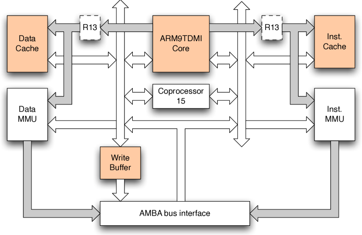
Figure 1: Simplified block diagram of the ARM920T. Gray arrows are address buses/connections. White arrows are data buses/connections. Both are 32 bits wide. Coprocessor 15 hosts control registers for the caches and the MMUs. Actually Register R13 (which should not be confused with the ARM9TDMI r13 register presented in section 3.1) is not duplicated and is located in Coprocessor 15. It hosts a process ID used for virtual address to physical address translation. Some blocks like the Write back Physical TAG RAM and various debug and/or coprocessor interfaces are not shown.

3.1 Reduced Instruction Set Computer Architecture

The ARM architecture is a Reduced Instruction Set Computer (RISC) architecture. The instruction set consists of fixed size instructions and a few simple addressing modes. There are $16$ general purpose registers $r_{0}$ to $r_{15}$, specialized memory transfer instructions (load/store), and data-processing instructions that operate on registers only. Other interesting features are multiple load/store instructions and conditional execution of instructions (to improve data and execution throughput).

Three of the general purpose registers are used in a specialized way. Register $r_{13}$ is the stack pointer (we use sp in the sequel to refer to this register). Register $r_{14}$ is the link register (lr in the sequel) and hosts the return address of function calls. Register $r_{15}$ is the program counter (pc in the sequel).

An instruction is defined by a mnemonic (e.g., mov) and the operands. In the sequel, we let ${\cal R}=\{r_{0},\cdots,r_{12},$ $sp,lr,pc\}$ be the set of registers of the architecture and ${\cal I}$ be the (finite) set of RISC instructions.

3.2 Execution Pipeline

The ARM920T uses a 5-stage execution pipeline, the purpose of which is to execute concurrently the different tasks (Fetch, Decode, Execute, Memory, Writeback) needed to perform an instruction. The (normal) flow of instructions in the pipeline is shown in Fig. 2.

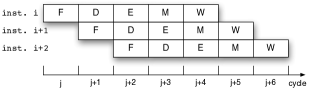
Figure 2: Pipeline of the ARM920T: Instruction is fetched in F. Instruction decode and operand register accesses are done in D. Execution is done in E. Load/store instructions do their memory accesses in M. Results are written back to registers in W.

This optimal flow may be slowed down when pipeline stalls occur. Most of the time, two independent consecutive instructions do not incur a stall and the throughput is 1 instruction/cycle. However in certain cases stalls can occur.

Figure 3: Load delay pipeline hazard.

Assume instruction ldr r1,[sp,#0] is followed by add r0,r1,#1: the first instruction loads register $r_{1}$ (with the content of a memory cell) and the second uses $r_{1}$ to compute r0. This sequence of instructions brings about a load delay depicted on Fig. 3. One stall cycle is inserted before processing instruction add r0,r1,#1 because the load instruction produces the operand needed ($r_{1}$) at the E stage of the add instruction at the end of its M stage.

Sometimes the target address of a branch instruction is produced at the end of the E stage (e.g., conditional branching that needs the result of a comparison operation). The ARM920T does not implement any branch prediction mechanism. As a consequence fetching the next instruction can only be done after the branch instruction has completed the E stage: this causes a branch delay depicted Fig. 4 that results in 2 stall cycles before the fetch of the branch target instruction can be performed.

Figure 4: Branch delay pipeline hazard.

3.3 Main Memory, Instruction and Data Cache, Write Buffer

Both instruction and data caches have the same architecture. They are 16KB, 8-ways set associative caches. There are 64 sets and 512 32 bytes long lines. Replacement policy may be set to pseudo-random or round-robin (FIFO). Both caches implements allocate-on-read-miss i.e., a data is inserted in the cache if missing when a read is performed.

The data cache may be configured in write-through (when data in the cache is modified, it is immediately written to the main memory) or write-back (modified cached data are only written to main memory when needed) but does not implement allocate-on-write-miss: if non cached data is written to, they are not cached but instead written to main memory directly. So, even if configured in write-back, a write miss acts as a write-through. Each data cache line has 2 dirty bits (indicating that a cached item has been modified since last cached), one per half-line, to indicate the half-line must be written back when it is replaced.

A 16-word write buffer helps to reduce stalls when a write to the main memory occurs because of a write miss or, if the cache is configured in write-back, when a dirty line has to be replaced. The write buffer is organized in 4 half-line entries to allow cache write-back on a half-line basis.

Finally, transfers between the caches and main memory are serialized and the bus abstracted away.

4 Program Semantics

In this section we present the formal semantics for the execution of binary programs. We make the following assumptions on the binary programs we analyse:

• the termination of a program does not depend on input data, i.e., a program terminates for all input data; and

• reference to stack values is via the specialised register sp only.

• references to memory cells are independant from input data. This ensures that when an instruction computes the address of a memory cell, it is always defined.

• The programs do not contain recursive calls.

4.1 Notations

We let $\mathbb{B}=\{\mbox{{true}},\mbox{{false}}\}$. We have already introduced some notations: ${\cal R}$ is the set of registers of the hardware, ${\cal I}$ is the (finite) set of instructions the hardware can perform, and ${\cal M}$ the (finite) set of main memory cells the program can access. In the sequel we will introduce a set of predicates ${\cal P}$ and for $x\in{\cal R}\cup{\cal P}\cup{\cal M}$ (set of registers or predicates or memory cells), $[\![x]\!]$ denotes the content of $x$. A program state $s$ is a valuation of the variables in ${\cal R}\cup{\cal P}\cup{\cal M}$ i.e., a mapping from ${\cal R}\cup{\cal P}\cup{\cal M}$ to ${\cal D}$ where ${\cal D}$ is a finite set e.g., 32-bit integers. We let ${\cal S}$ be the set of program states.

As program instructions are located in main memory, we define the set of labelled instructions ${\cal L}{\cal I}={\cal M}\times{\cal I}$ to be the set of pairs $(\ell:i)$ indicating that instruction $i$ is stored at address $\ell$ in main memory. Consequently, a program $P$ is simply a subset (necessarily finite) of ${\cal L}{\cal I}$. We use the notation $<\!\!\iota\!\!>:{\cal S}\rightarrow{\cal S}$ to denote the semantics of instruction $\iota\in{\cal L}{\cal I}$.

Remark 1

The semantics is defined on labelled instructions which means that the semantics itself may depend on the address the instruction is stored at. This is actually the case for some instructions like 12: ldr r0,[pc,#4] the semantics of which is “load register $r_{0}$ with the content of the memory cell located at offset $4$ from the current value of pc”, i.e., at address $12$.

4.2 Example Program

As a running example we take the binary program FIBO of Listing 1. It has been compiled (gcc) and de-assembled (objdump) using the GNU ARM tools from Codesourcery [12]. It computes $\textit{Fib}(30)$ the Fibonacci number $u_{30}$ with $u_{0}=1$, $u_{1}=1$ and $u_{n}=u_{n-1}+u_{n-2},n\geq 2$. A program is stored in memory and the memory address of each instruction is the leftmost decimal number. Each program has a designated initial instruction $\iota_{0}=(\ell_{0},i_{0})$ and $[\![\emph{pc}]\!]=\ell_{0}$ at the beginning of the execution of the program.

To give the semantics of programs, we assume there is a set of variables ${\cal P}=\{le,gt,\cdots\}$ to hold the truth values of the predicates used in the conditional instructions of the program.

The semantics of program FIBO is given in terms of assignments to registers (on the right-hand side of each instruction in Listing 1). Each instruction assigns a new value to register pc: except for branching instructions the assignment is $[\![pc]\!]:=[\![pc]\!]+4$ and we omit it in this case. A comparison operator (e.g., line 24) sets the truth value of the predicates that are used later in the program (e.g., eq for instruction at line 24). The main loop of the computation is between line 24 and 52; notice that this optimized program (compiled with option -O2) computes $u_{n+2}$ in each round of this loop ($r_{2}$ holds the value of $n$ and is incremented twice in the body of the loop).

⬇

0 <main>: /*starts at address 0;*/

0 mov r1,#30 $[\![r_{1}]\!]:=30$

4 mov r2,#2 $[\![r_{2}]\!]:=2$

8 add r1,r1,#1 $[\![r_{1}]\!]:=[\![r_{1}]\!]+1$

12 add r2,r2,#1 $[\![r_{2}]\!]:=[\![r_{2}]\!]+1$

16 mov r0,#0 $[\![r_{0}]\!]:=0$

20 mov r3,#1 $[\![r_{3}]\!]:=1$

24 cmp r2,r1 $[\![eq]\!]:=([\![r_{2}]\!]=[\![r1]\!])$

28 add r0,r0,r3 $[\![r_{0}]\!]:=[\![r_{0}]\!]+[\![r3]\!]$ /**/

32 bxeq lr if $([\![eq]\!])$ $[\![pc]\!]:=[\![lr]\!]$ else $[\![pc]\!]:=36$

36 add r2,r2,#1

40 add r2,r2,#1

44 add r3,r3,r0 $[\![r_{3}]\!]:=[\![r_{3}]\!]+[\![r_{0}]\!]$

48 cmp r2,r1 $[\![eq]\!]:=([\![r_{2}]\!]=[\![r1]\!])$

52 add r0,r0,r3

56 bne 24 if $(\neg[\![eq]\!])$ $[\![pc]\!]:=24$ else $[\![pc]\!]:=60$

60 bx lr $[\![pc]\!]:=[\![lr]\!]$

Listing 1: Program FIBO: computes Fibonacci $30$

4.3 Abstract Hardware Model

The real hardware (Section 3) consists of the pipelined processor, instruction and data caches, write buffer and the main memory of the computer. We abstract away the details of the communication medium (AMBA bus, MMU). We choose to treat the content of the main memory as a component of the program state and thus it is not part of the state of the hardware. The same remark applies for the register and we consider they are part of the program state. A state of the hardware is then defined by the states of the different stages of the pipeline and the states of the caches.

As we are only interested in computing execution times, we can consider that the hardware is an abstract machine $H$ that reads sequences of triples $(\iota,A,d)\in{\cal L}{\cal I}\times{\cal M}\times\mathbb{B}$ and outputs the time it takes to process such a sequence. A triple $(\iota,A,d)$ consists of a (labelled) instruction $\iota=(\ell:i)$ with $\ell\in{\cal M}$ and $i\in{\cal I}$ that references a set of (main memory) addresses in $A$ and is performed if $d=\mbox{{true}}$; if $d=\mbox{{false}}$ the instruction is a conditional instruction and the condition the instruction depends on last evaluated to false. Such triples (and sequences thereof) contain enough information to compute the execution time:

• pipeline stalls (see 3.2) can be inferred from the first component of the triple $\iota$ that contains the full text of the instruction and thus the read/written registers and the value of $d$ (whether the instruction is executed or not);

• cache hits/misses (see 3.3) are completely determined by the set $A$.

Examples of instructions for program FIBO (Listing 1) are 0: mov r1,#30 and 32:bxeq lr. Notice that there is no need for actual register values in $H$ neither for performing the real computation as the timing of instructions in the pipeline and the cache is fully determined by the instruction (and its location in memory), whether it is performed or not (there are conditional instructions), the registers read from/written to and the memory addresses used in the instruction. The fact that there is no branch prediction in the pipeline of the hardware in the ARM920T makes things simpler but the framework we present extends to the case with branch prediction (see [10]).

The execution time of a sequence of triples also depends on the initial state $\gamma$ of the hardware $H$. Given a finite sequence $w=q_{0}q_{1}q_{2}\cdots q_{n}\in({\cal L}{\cal I}\times{\cal M}\times\mathbb{B})^{*}$ and an initial state $\gamma$ of $H$, $\mbox{{time}}_{H}(\gamma,w)$ is the execution time of $w$ from initial state $\gamma$ of $H$. It can be defined precisely using for instance the HDL model of the hardware. Notice that at this point, we do not require sequences of triples to be actual sequences produced by program $P$.

4.4 Trace Semantics of a Program

The execution of a program can be defined by an alternating sequence of program states and instructions. A run of a program $P$ is a sequence $\varrho=s_{0}\;\iota_{0}\;s_{1}\;\iota_{1}\;s_{2}\;\iota_{2}\quad\cdots\quad s_{n-1}\;\iota_{n-1}\;s_{n}$ where $s_{k}$ is a program state and $\iota_{k}=(\ell_{k}:i_{k})$ is a labelled instruction with $\ell_{k}=s_{k}(pc)$ and such that $s_{k+1}=<\!\!\iota_{k}\!\!>(s_{k})$. We let $\textit{Runs}(P)$ be the set of runs of $P$.

The trace, $\textit{TR}(\varrho)$, of the run $\varrho$ is the sequence $q_{0}q_{1}q_{2}\cdots q_{n}\in({\cal L}{\cal I}\times{\cal M}\times\mathbb{B})^{*}$ with $q_{i}=(\iota_{i},A_{i},d_{i})$ where $A_{i}$ is the set of memory addresses referenced by instruction $\iota_{i}$ in state $s_{i}$ and $d_{i}\in\mathbb{B}$ indicates whether the instruction is actually executed. For instance, instruction ldr r0,[sp, #4] from a program state $s$ with $s(sp)=12$ references address $16$ and is performed (unconditional). Instruction 128: addle r1,r1,#1 is performed only if the last comparison set the predicate le true and from program state $s$ the next triple in the trace is (128: addle r1,r1,#1, $\varnothing$, $s(le))$. As there are multiple load and store instructions, we need sets of addresses to represent the memory cells referenced by an instruction: instruction stm sp,{r0,r1} references addresses $12$ and $8$.

The execution time of a run $\varrho$ of $P$ from initial state $\gamma$ of $H$ is defined by $\mbox{{time}}_{H}(\gamma,\textit{TR}(\varrho))$.

Program $P$ has a set of initial states $I$ (where $[\![\emph{pc}]\!]$ gives the initial instruction of $P$) and the contents of the registers, predicates and main memory can be in a finite set of values. Notice that there can be many initial states as the input data of $P$ can range over large sets. $P$ also has a set of final states, $F$, and we assume it can be defined using the value of register pc which gives the last instruction of $P$. The language ${\cal L}_{I}^{F}(P)$ of $P$ is the set of traces generated by runs of $P$ that start in $I$ and end in $F$ i.e., ${\cal L}_{I}^{F}(P)=\{\textit{TR}(\varrho)\ |\ \varrho=s_{1}\iota_{1}\cdots s_{n-1}\iota_{n-1}s_{n},\varrho\in\textit{Runs}(P),s_{1}\in I,s_{n}\in F\}$. As we assume that $P$ always terminates for any input data, this language is finite (because the set of memory contents is finite).

5 Computation of the WCET

5.1 Modular Definition of WCET

Given a run $\varrho$ of $P$, the execution time of $\varrho$ on $H$ from state $\gamma$ only depends on $\textit{TR}(\varrho)$. This implies that the WCET of $P$ only depends on ${\cal L}_{I}^{F}(P)$ and the initial state $\gamma$ of $H$. Consequently if ${\cal L}_{I}^{F}(P)$ is finite

$$\text{WCET}(P,H)=\max_{w\in{\cal L}_{I}^{F}(P)}\mbox{{time}}_{H}(\gamma,w)\mathpunct{.}$$ (1)

The computation of $\text{WCET}(P,H)$ thus amounts to ($i$) generating ${\cal L}_{I}^{F}(P)$, ($ii$) feeding $H$ with each $w\in{\cal L}_{I}^{F}(P)$ and tracking the maximal execution time. This gives a modular way of computing $\text{WCET}(P,H)$ since a generator for ${\cal L}_{I}^{F}(P)$ and the behaviour of the abstract hardware $H$ to be fed with ${\cal L}_{I}^{F}(P)$ can be given independently of each other.

5.2 Extended Domain Abstraction

In order to take into account all the possible values of the input data, we use an extended domain for the values of the main memory cells. We assume here that the values of the registers and predicates are known in the initial state.

Let ${\cal D}_{\bot}={\cal D}\cup\{\bot\}$ be the extended domain with $\bot$ the unknown value. The semantics of instructions is extended to this extended domain: for instance, the semantics of add r0,r1,#1 is given by

$$[\![r_{0}]\!]=\textit{ $\bot$ if $([\![r_{1}]\!]=\bot)$ and $[\![r_{1}]\!]+1$ otherwise}\mathpunct{.}$$

The semantics of comparison instructions e.g., cmp r0,r1 is extended as well to ${\cal D}_{\bot}$ e.g., for instruction 24 of program FIBO,

$$[\![eq]\!]=\bot\textit{ if $(([\![r_{0}]\!]=\bot)$ or $([\![r_{1}]\!]=\bot))$ and ($[\![r_{0}]\!]=[\![r_{1}]\!]$) otherwise}\mathpunct{.}$$

When a conditional instruction is encountered and the condition is $\bot$, the extended semantics of the instruction considers two successors: one where the condition is true and the other where the condition is false. If a branching instruction like $\mathtt{bx\ lr}$ is encountered and $[\![lr]\!]=\bot$ the next instruction is undefined (we can encode this by jumping to a special “error” state but this situation will not occur in the sequel).

We may now define an extended symbolic semantics for a program $P$, and starting from an initial state $s_{0}:{\cal R}\cup{\cal P}\cup{\cal M}\rightarrow{\cal D}_{\bot}$, the symbolic semantics define a set of runs (non-determinism may arise if some conditions are tested and unknown).

Assume that the values of the registers and predicates are fixed in the initial program and given by $s_{0}({\cal R}\cup{\cal P})$ and the input data is $d$: the initial state of the memory is $s_{0}(d)$ with $s_{0}(d):{\cal M}\rightarrow D$. The initial state of the program is thus defined by $s_{0}({\cal R}\cup{\cal P})\cdot s_{0}(d)$.

Define $s_{0}^{\bot}:{\cal R}\cup{\cal P}\cup{\cal M}\rightarrow D_{\bot}$ by: $s_{0}^{\bot}(x)=s_{0}(x)$ for $x\in{\cal R}\cup{\cal P}$ and $s_{0}^{\bot}(y)=\bot$ for $y\in{\cal M}$.

The important property of the extended semantics is $(\pi)$: if $\varrho$ is a run of $P$ from state $s_{0}(d)$, then $\varrho$ is a run of $P$ from $s_{0}^{\bot}$ in the extended symbolic semantics.

In the sequel we write ${\cal L}_{\bot}(P)$ for ${\cal L}_{\{s_{0}^{\bot}\}}^{F}(P)$ and $\text{WCET}_{\bot}(P,H)=\max_{w\in{\cal L}_{\bot}(P)}\mbox{{time}}_{H}(\gamma,w)$. The property $(\pi)$ of the symbolic semantics implies that ${\cal L}_{I}^{F}(P)\subseteq{\cal L}_{\bot}(P)$ and by language inclusion we have

$$\text{WCET}(P,H)=\max_{w\in{\cal L}_{I}^{F}(P)}\mbox{{time}}_{H}(\gamma,w)\leq\max_{w\in{\cal L}_{\bot}(P)}\mbox{{time}}_{H}(\gamma,w)=\text{WCET}_{\bot}(P,H)\mathpunct{.}$$ (2)

We can thus reduce the computation of (an upper bound of the) $\text{WCET}(P,H)$ to a symbolic simulation of program $P$ on the extended domain ${\cal D}_{\bot}$ from a unique initial state $s_{0}^{\bot}$.

As we have assumed that termination does not depend on the input data, but is guaranteed for each program $P$, the symbolic simulation of $P$ on the extended domain terminates as well. Each test that ensures termination in $P$ cannot evaluate to $\bot$ because otherwise it would depend on the input data and this would contradict assumption (A1).

5.3 WCET Computation as a Reachability Problem

We can reduce the computation of the WCET to a reachability problem on a network a timed automata. Indeed, as ${\cal L}_{\bot}(P)$ is finite, it can be generated by a finite automaton $\textit{Aut}(P)$. The hardware $H$ (including pipeline, caches and main memory) can be specified by a network of timed automata $\textit{Aut}(H)$ (formal models are given in Section 8). Feeding $H$ with ${\cal L}_{\bot}(P)$ amounts to building the synchronised product $\textit{Aut}(H)\times\textit{Aut}(P)$. On this product we define final states to be the states where the last instruction of $P$ flows out of the last stage of pipeline. Assume a fresh clock $x$ is reset in the initial state of $\textit{Aut}(H)\times\textit{Aut}(P)$. The WCET of $P$ on $H$ is then the largest value, $\max(x)$, that $x$ can take in a final state of $\textit{Aut}(H)\times\textit{Aut}(P)$ (we assume that time does not progress from a final state).

We can compute $\max(x)$ using model-checking techniques with the tool Uppaal [8] (see Section 9). To do this, we check a reachability property “(R): Can we reach a final state with $x\geq K$?” on $\textit{Aut}(H)\times\textit{Aut}(P)$. If the property is true for $K$ and false for $K+1$, $K$ is the WCET of $P$. We can compute this maximal value using the sup operator that gives the maximal value a clock can have in a reachable state.

Notice that to do this we have to explore the whole state space of $\textit{Aut}(H)\times\textit{Aut}(P)$. This means that to handle large case studies, we need to reduce the state space as much as possible.

An important point to notice is that the tightness of the WCET we compute depends on an accurate description of $H$. The more precise (time-wise) $\textit{Aut}(H)$ is, the more precise the computed WCET will be. It is thus not reasonable to take a very abstract $H$ (e.g., with caches that always miss) as it will give poor WCET estimates. We can still have some control on the automaton $\textit{Aut}(P)$ that generates the traces to be fed to $\textit{Aut}(H)$. Indeed, we should avoid generating two runs with the same trace as it will give the same WCET (from the same initial state of $H$). This means that minimizing $\textit{Aut}(P)$ can effectively reduce the state space (at least the number of paths explored in the product $\textit{Aut}(H)\times\textit{Aut}(P)$). In the next section we describe how to compute a reduced program $P^{\prime}$ that generates the same set of traces as $P$.

6 Slicing

Program Slicing was introduced by Mark Weiser [32] in 1984. The purpose of program slicing is to compute a program slice (by removing some statements of the original program) s.t. the slice computes the same values for some variables at some given statements. Program slicing is often used for checking properties of programs. The reader is refered to [31] for a survey on the principles of (static and dynamic) slicing.

6.1 Overview of Program Slicing

In this section, we assume that we have the control flow graph of $P$, $CFG(P)$, which is a directed graph, the nodes of which are in $P$. $CFG(P)$ has a single entry node (initial instruction of the program $P$) and a single exit node (that indicates the end of program $P$). An example of a CFG for the Fibonacci program of Listing 1 is given in Figure 5.

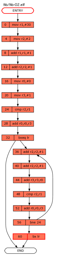
Figure 5: CFP for Program of Listing 1.

A slice criterion ${\cal C}$ for $P$ is a subset $I^{\prime}\subseteq P$, and for each instruction $\iota\in I^{\prime}$ an associated subset of “variables” ${\cal V}(\iota)\subseteq{\cal R}\cup{\cal P}\cup{\cal M}$. We assume that ${\cal V}(\iota)$ is actually included in the set of registers that the instruction operates on but this is inessential. For instance, a slice criterion for program $FIBO$ of Figure 5 can be instruction $48:\mathtt{cmp\ r2,r1}$ and associated set $\{r_{1},r_{2}\}$.

Given input data $d\in{\cal D}$, we write $\textit{run}(P,d)$ to denote the (unique) run of $P$ on $d$. Let $S\subseteq P$. The runs of $P$ and $S$ on input data $d\in{\cal D}$ are denoted

$$\textit{run}(P,d) = s_{1}\iota_{1}s_{2}\iota_{2}\cdots s_{k}\iota_{k}\cdots s_{n}\iota_{n}s_{n+1}$$

$$\textit{run}(S,d) = s^{\prime}_{1}\iota^{\prime}_{1}s^{\prime}_{2}\iota^{\prime}_{2}\cdots s^{\prime}_{k}\iota^{\prime}_{k}\cdots s^{\prime}_{m}\iota^{\prime}_{m}s^{\prime}_{m+1}$$

Define the projection $\textit{proj}(s,\iota)$ for a pair $(s,\iota)\in{\cal L}{\cal I}$ by:

$$\textit{proj}(s,\iota)=\begin{cases}\varepsilon\text{ if $\iota\not\in S$ }\\ (\textit{proj}_{{\cal V}(\iota)}(s),\iota)\text{ otherwise}.\end{cases}$$

i.e., instructions not in the subset $S$ are ignored (replaced by $\varepsilon$, the empty word) and for instructions in $S$ we keep the projection on ${\cal V}(\iota)$ of the program state. proj is extended in the natural way to traces and we let $\textit{proj}^{*}(\varepsilon)=\varepsilon$ and $\textit{proj}^{*}(w.(s,\iota))=\textit{proj}^{*}(w).\textit{proj}^{*}(s,\iota)$ with $s$ a program state and $\iota\in{\cal L}{\cal I}$.

$S$ is a slice of $P$ for the slice criterion ${\cal C}$ if it satisfies, for every input data $d\in{\cal D}$:

1. if $P$ terminates on input $d$ then $S$ terminates on input $d$ and

2. $\textit{proj}^{*}(run(P,d))=\textit{proj}^{*}(run(S,d))$. Notice that by definition of proj, all the instructions of $S$ are in $\textit{proj}^{*}(run(S,d))$ but the projection restricts the set $s^{\prime}_{k}$ to the variables in ${\cal V}(\iota^{\prime}_{k})$.

In the sequel we recall how to (effectively) compute a slice for $P$ given a slice criterion ${\cal C}$.

6.2 Prerequisites for Computing a Program Slice

The computation of a slice is based on an iterative solution of dataflow equations on the set of relevant variables for each instruction in the CFG of $P$. The relevant variables for an instruction are the variables read from/written to by the instruction. Due to the particular nature of binary programs, the knowledge of relevant variables for an instruction might not be explicit: consider the instruction $\textit{foo}=\texttt{str r0,[sp,\#4]}$ again. This instruction reads register $r_{0}$ and writes to the “variable” which is the memory cell at location $[\![\textit{sp}]\!]+4$. This value is not known at compile time. The previous instruction writes in the stack which is particular region of the main memory. Other instructions like 16: str r2,[r1, r3 lsl #2] might (read or) write to arbitrary memory cells: in this case the memory cell with address $[\![r_{1}]\!]+([\![r_{3}]\!]<<2)$.

In our approach we make the following choice:

1. we consider that the content of the main memory outside the stack is always $\bot$; this means that we do not need to store the main memory content into the program state as it is constant.

2. by assumption (A2), every access to a stack value is via register sp. We use the term stack reference for instructions that read/write sp and main memory reference for the other memory accesses.

3. for an instruction which has a stack reference, (e.g., in str r0,[sp,#4]), we only know the actual offset at runtime. To define the referenced variables, we introduce a variable stack. This means that we track the stack content in the state of the program and this variable is updated by instruction that do stack references. The previous instruction thus reads $r_{0}$ and $sp$ and writes to stack.

This enables us to define formally the set of referenced and defined variables for each instruction, which is mandatory in order to compute automatically a slice.

Given instruction $i\in{\cal I}$ the set of read from (REF) and written to (DEF) variables is given by:

• for instructions that do not make main memory references or stack references, e.g., $i=\texttt{add r2,r1,\#1}$ we have $REF(i)=\{r_{1}\}$ and $DEF(i)=\{r_{2}\}$.

• for instructions that make stack references, e.g., $i=\mathtt{push(r_{0},r_{1})}$, we define $REF(i)=\{r_{0},r_{1},sp\}$ and $DEF(i)=\{sp,stack\}$.

• for instructions that make main memory references, we assume the content of main memory is $\bot$. For an instruction like $i=\texttt{str r2,[r1, r3 lsl \#2]}$ we thus have $REF(i)=\{r_{1},r_{2},r_{3}\}$ and $DEF(i)=\varnothing$. Indeed, even if the memory location $[\![r_{1}]\!]+([\![r_{3}]\!]<<2)$ is written to, the new content of the main memory does not depend on the values of the registers and thus we can omit it in the set of $DEF$ variables.

6.3 Step 1: A Slice for Values of Register sp.

The first task we perform on a binary program $P$ is to compute the possible values of the stack references (values of sp).

We can compute the possible values of the stack pointer sp for a given instruction using a slice criterion ${\cal C}$: ${\cal C}$ contains all the instructions that read/write the variable sp i.e., all the instructions s.t. $DEF(i)\cap\{sp\}\neq\varnothing$ or $REF(i)\cap\{sp\}\neq\varnothing$ .

We compute a slice of $P$ for ${\cal C}$, $S_{\cal C}(P)$ using the standard definition of data dependence and control dependence (see [31]). Once computed, we do a symbolic simulation of $S_{\cal C}(P)$ and track the values of sp encountered for each instruction in ${\cal C}$.

As we have assumed (A1) that termination does not depend on the input data, but is guaranteed for each program $P$, the symbolic simulation of the slice $S_{\cal C}(P)$ on the extended domain terminates as well. During the course of the symbolic simulation, we track the values of the sp register for each stack reference instruction. At the end of the simulation, we obtain the set of possible values for sp at each stack reference instruction. Because of the property of the slice, and the symbolic simulation in the extended domain (superset of the set of runs) we can ensure that the set of sp values we obtain for each instruction is a superset of the set actual values in $P$.

Limitations.

The previous approach works correctly if the stack is referenced only via the register sp, assumption (A2). This is ensured by the API of the compilers from C/C++ to ARM for instance and thus is a perfectly reasonable assumption.

We can take advantage of the computation performed previsouly to narrow the $DEF$ and $REF$ variables for each instruction in $P$. Assume for instruction $\iota=\texttt{4: str r0,[sp,\#4]}$, the set of possible values of sp is $\{12,16\}$. What we know about the written to variables is more precise than being somewhere in the stack. We know that variables at index $12$ and $16$ may be written to, and this instruction does not modify other stack items at other offsets. We thus refine the definitions of $REF$ and $DEF$ for instruction $\iota$ by setting: $REF^{*}(\iota)=\{r_{0},sp\}$ (unchanged in this case) and $DEF^{*}(\iota)=\{stack_{12},stack_{16}\}$. This more precise definitions will result in smaller subsequent slices as they will introduce less data dependences in the CFG of a program.

In the sequel, we show how to use program slicing to compute a WCET-equivalent program. In the next section, we also show how to iteratively use program slicing to build the CFG of arbitrary assembly (unstructured) programs.

6.4 Step 2: Using Program Slicing to Compute a WCET-Equivalent Program

As in the previous subsection, assume that we have the complete CFG of $P$ (building this CFG is addressed in Section 7). Equation 1 implies that for any two programs $P$ and $P^{\prime}$,

$${\cal L}_{\bot}(P)={\cal L}_{\bot}(P^{\prime})\Longrightarrow\text{WCET}_{\bot}(P,H)=\text{WCET}_{\bot}(P^{\prime},H)\mathpunct{.}$$ (3)

What we would like to do is to compute such a WCET-equivalent program $P^{\prime}$ which (hopefully) operates on a reduced subset of the set of registers ${\cal R}$ yet contains enough information to generate ${\cal L}_{\bot}(P)$.

Using the previously computed attributes $REF^{*}$ and $DEF^{*}$, we can compute a WCET-equivalent program using an ad-hoc slice criterion ${\cal C}^{\prime}$: ${\cal C}^{\prime}$ contains ($i$) all the instructions that perform main memory transactions (including the stack), and each instruction has the associated set of variables that defines the memory location, ($ii$) all the conditional instructions $\iota$ with associated set of variables ${\cal V}(\iota)\ni p$ if $p$ is the condition of the instruction. For instance, instruction $j=(\texttt{16: ldr r2,[r1, r3 lsl \#2]})$ is in ${\cal C}^{\prime}$ and we have to track the values of registers ${\cal V}(j)=\{r_{1},r_{3}\}$ since the memory address is defined by $r_{1}$ and $r_{3}$. For an instruction like $l=(\texttt{12:addle r1,r2,\#1})$ we set ${\cal V}(l)=\{le\}$.

Let $S_{{\cal C}^{\prime}}(P)$ be the slice computed using the criterion ${\cal C}^{\prime}$. What we want is to generate the language ${\cal L}_{\bot}(P)$ using the slice. For each instruction $\iota\in P$ we define a corresponding abstracted $\alpha(\iota)$ as follows:

• if $\iota\in P\cap S_{{\cal C}^{\prime}}(P)$ then $\alpha(\iota)=\iota$;

• for the other instructions $\iota\in P\setminus S_{{\cal C}^{\prime}}(P)$, $\alpha(\iota)=\iota_{nop}$ where $\iota_{nop}$ denote the instruction with the exact same syntax as $\iota$ but the semantics of $\iota_{nop}$ is $[\![pc]\!]:=[\![pc]\!]+4$. As the syntax of $\iota$ is identical to $\iota_{nop}$, this alos preserves the $REF$ and $DEF$ attributes.

We let $\alpha(P)$ be the program that comprises of instructions $\alpha(\iota),\iota\in P$. Notice that $alpha$ is one-to-one mapping and thus we can consider $\alpha^{-1}$ when needed.

We can now prove the following Lemmas:

Lemma 1

Let $\varrho=s_{0}^{\bot}\iota_{0}s_{1}\iota_{1}s_{2}\iota_{2}\ \cdots\ \iota_{k-1}s_{k}$ be a run of $P$. The run $\varrho^{\prime}={s^{\prime}}_{0}^{\bot}\alpha(\iota_{0})s^{\prime}_{1}\alpha(\iota_{1})s^{\prime}_{2}\alpha(\iota_{2})$ $\cdots\ \alpha(\iota_{k-1})s^{\prime}_{k}$ is in $\alpha(P)$ and $\textit{TR}(\varrho)=\textit{TR}(\varrho^{\prime})$.

Proof

We prove the Lemma by induction. The induction hypothesis (IH) is: for runs of length $k$, $\textit{TR}(\varrho)=\textit{TR}(\varrho^{\prime})$ and $s^{\prime}_{k}=\textit{proj}_{{\cal V}(\iota_{k})}(s_{k})$ if $\iota_{k}$ is the instruction following $\iota_{k-1}$ and $\iota_{k}$ is in the slice, and $s^{\prime}_{k}=\textit{proj}_{\{pc\}}(s_{k})$ otherwise. The Lemma is true for runs of length $0$. Assume we have a run of length $k+1$ i.e., $\varrho=s_{0}^{\bot}\iota_{0}s_{1}\iota_{1}s_{2}\iota_{2}\ \cdots\ \iota_{k-1}s_{k}\iota_{k}s_{k+1}$. First notice that instruction $\alpha(\iota_{k})$ is a successor of $\alpha(\iota_{k-1})$ as the CFG of $\alpha(P)$ is isomorphic to $CFG(P)$. We can compute the triple $(x,A,d)$ and $(x^{\prime},A^{\prime},d^{\prime})$ added to the trace of $\varrho$ and $\varrho^{\prime}$ after instructions $\iota_{k}$ and $\alpha(\iota_{k})$:

• the first component of the triple is the same as $alpha(\iota_{k})$ and $\iota_{k}$ have exactly the same syntax (and location); hence $x=x^{\prime}$.

• for the second component, memory references, there are two cases:

  • either $\iota_{k}$ does not make any memory transfer and references only registers. The same applies to $\alpha(\iota_{k})$ and the second component is the empty set;

  • or $\iota$ has memory references. In this case, the registers that generate the memory references are in the slice, and thus the values at $s_{k}$ and $s^{\prime}_{k}$ coincide by the “projection” property of the slice.

  In each case $A=A^{\prime}$.

• the third components $d,d^{\prime}$ are the values of the conditions of the instruction $\iota_{k}$ and $\alpha(\iota_{k})$. If the instruction $\iota_{k}$ is unconditional, $d=\mbox{{true}}$ and $d^{\prime}=\mbox{{true}}$. Otherwise, the two instructions have the condition $c$. As $\iota_{k}$ is conditional, the condition is in the slice (by definition of the slice) and thus $s_{k}(c)=s^{\prime}_{k}(c)$. Hence $d=d^{\prime}$.

This proves that $\textit{TR}(\varrho)=\textit{TR}(\varrho^{\prime})$ and completes the proof. ∎

Lemma 2

Let $\varrho^{\prime}={s^{\prime}}_{0}^{\bot}\iota^{\prime}_{0}s^{\prime}_{1}\iota^{\prime}_{1}s^{\prime}_{2}\iota^{\prime}_{2}$ $\cdots\iota_{k-1}s^{\prime}_{k}$ be a run of $\alpha(P)$. There is a run $\varrho=s_{0}^{\bot}\iota_{0}s_{1}\iota_{1}s_{2}\iota_{2}\cdots\iota_{k-1}s_{k}$ of $P$ with $\iota^{\prime}_{i}=\alpha(\iota_{i})$ and $\textit{TR}(\varrho)=\textit{TR}(\varrho^{\prime})$.

Proof

The proof relies on the following fact: every instruction in $P$ that has more than one successor is conditional and thus is in the slice. Consequently, given two instructions $\iota^{\prime}_{j}=\alpha(\iota_{j})$ and $\iota^{\prime}_{j+1}=\alpha(\iota_{j+1})$ in the slice, there is a unique sequence (with no loop) of instructions in $CFG(P)$ between $\iota_{j}$ and $\iota_{j+1}$. This shows that there is a (unique) run in $P$ defined by $\iota_{j}=\alpha^{-1}(\iota^{\prime}_{j})$. Using the result of Lemma 1 completes the proof. ∎

By combining Lemma 1 and 2 we obtain:

Theorem 6.1

$\text{WCET}_{\bot}(P,H)=\text{WCET}_{\bot}(\alpha(P),H)$.

Proof

Lemmas 1 and 2 imply that ${\cal L}_{\bot}(P)={\cal L}_{\bot}(\alpha(P))$ and by Equation 3, the result follows. ∎

When we do program slicing, many operations on registers are avoided if they do not influence the control flow. The result is that $\alpha(P)$ generates less states than $P$: assume register $r_{4}$ is never used in $\alpha(P)$ but used in $P$, then all the states of $P$ that differs only on $r_{4}$ are collapsed into the same state. This also means that the automaton $Aut(\alpha(P))$ that generates ${\cal L}_{\bot}(\alpha(P))$ will have less states than $Aut(P)$. Quite often, some registers are not used at all or do not influence the control flow and this reduces drastically the number of states in $Aut(\alpha(P))$.

An example of a slice is given in Figure 6, for the Fibonacci program $FIBO_{0}$ compiled with option $O0$: only $12$ instructions out of $40$ need be really simulated and the variables in the sliced program are $\{pc,r_{0},r_{2},r_{3}\}$ and $3$ stack values.

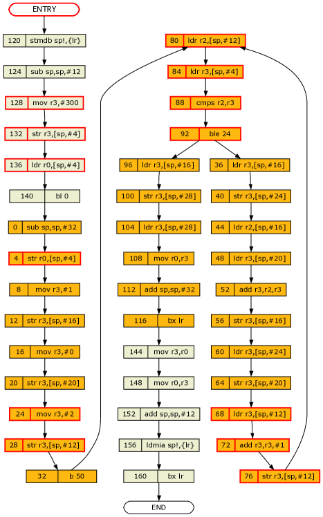
Figure 6: WCET-equivalent Slice for Program $FIBO_{0}$.

Another advantage of slicing is that we do not need to do loop unrolling because the registers and instructions that control the loop bounds are automatically preserved by the slice.

In Table 1, Section 10, column “Abs” ($a/b$) gives, for each program $P$, the number of nodes $a$ for which the simulation of an instruction is needed compared to the total number of nodes $b$ of $Aut(P)$.

This reduction has not only an effect on the state space (reduction of the number of paths explored) but also on the size of the representation of each state of $Aut(\alpha(P))$.

In the next section, we describe how we automatically compute the CFG of a program.

7 Computation of the CFG

To compute the CFG of a program, we iterate two phases:

1. Slice. We slice a partial CFG in order to compute the dynamically computed branch targets; we simulate the sliced program to determine these targets.

2. Expand: having determined the dynamically computed branch targets, we expand the partial CFG and repeat Step 1.

When the iteration terminates we have the CFG of the program. We limit the scope of our tool to non recursive programs, and this ensures that the previous iterative computation terminates.

We describe the process on an example of a Fibonnaci program $FIBO_{0}$ (compiled with option $-O0$) given in Listing 2. This program is composed of two functions, main and fib: main calls fib and at the end, fib returns. The computation would go like this: after instruction $8c$ in main, fib starts as $8c$ is “(b)ranch to $0$ and save return address to (l)ink register lr”. If at some point, instruction $74$ in fib is reached, lr should contain the return address in main i.e., $90$. It should also be noticed that the first instruction in main is to save on the stack, the return of the caller: push(lr). This is used at the end of main to return to the caller’s next instruction when the statement bx lr (“branch to the content of lr”) is performed right after popping the value of lr.

⬇

00000000 <fib>:

0: e24dd020 sub sp, sp, #32

4: e58d0004 str r0, [sp, #4]

8: e3a03001 mov r3, #1

12: e58d3010 str r3, [sp, #16]

16: e3a03000 mov r3, #0

20: e58d3014 str r3, [sp, #20]

24: e3a03002 mov r3, #2

28: e58d300c str r3, [sp, #12]

32: ea00000a b 50 <fib+0x50>

36: e59d3010 ldr r3, [sp, #16]

40: e58d3018 str r3, [sp, #24]

44: e59d2010 ldr r2, [sp, #16]

48: e59d3014 ldr r3, [sp, #20]

52: e0823003 add r3, r2, r3

56: e58d3010 str r3, [sp, #16]

60: e59d3018 ldr r3, [sp, #24]

64: e58d3014 str r3, [sp, #20]

68: e59d300c ldr r3, [sp, #12]

72: e2833001 add r3, r3, #1

76: e58d300c str r3, [sp, #12]

80: e59d200c ldr r2, [sp, #12]

84: e59d3004 ldr r3, [sp, #4]

88: e1520003 cmp r2, r3

92: dafffff0 ble 24 <fib+0x24>

96: e59d3010 ldr r3, [sp, #16]

100: e58d301c str r3, [sp, #28]

104: e59d301c ldr r3, [sp, #28]

108: e1a00003 mov r0, r3

112: e28dd020 add sp, sp, #32

116: e12fff1e bx lr

00000078 <main>:

120: e52de004 push {lr} ; [stmdb sp,lr] 124: e24dd00c sub sp, sp, #12 128: e3a03f4b mov r3, #300 132: e58d3004 str r3, [sp, #4] 136: e59d0004 ldr r0, [sp, #4] 140: ebffffdb bl 0 <fib> 144: e1a03000 mov r3, r0 148: e1a00003 mov r0, r3 152: e28dd00c add sp, sp, #12 156: e49de004 pop lr ; [ldmia sp,{lr}]

160: e12fff1e bx lr

Listing 2: $FIBO_{0}$

If we perform a first unfolding of the program, we obtain a partial CFG depicted in Fig. 7. In this CFG, the successor of instruction $116$ is unknown and thus the unfolding has a terminal node at this location. To compute the successor of this insruction we slice the partial CFG with the slice criterion ${\cal C}^{\prime\prime}=\{116\}$ and ${\cal V}(116)=\{lr\}$. The sliced program is composed of the red nodes i.e., instructions $140$ and $116$. Simulating this two-instruction program we get the possible value of lr at instruction $116$ which is $144$.

We can then extend the partial CFG to obtain the graph depicted on Fig. 8. We slice again to compute the successor of instruction $160$: the new slice (6 nodes) is depicted on Fig. 8 with the red nodes. We should here find that main handles the control back to its caller. To recognise this situation we use the following trick: we assume that before the first instruction of the program is performed, $[\![lr]\!]=\beta$ where $\beta$ is a special value that cannot correspond to any valid instruction. We can take for example $\beta=3$. When we compute a target which is $\beta$ we know that we have reached the end of the program because this returns to the caller. This situation occurs when we simulate the second slice and after the instruction 160:bx lr the program return to the caller.

The complete CFG for $FIBO_{0}$ is given in Fig. 9.

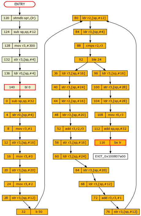
Figure 7: First Unfolding of the CFG of $FIBO_{0}$.

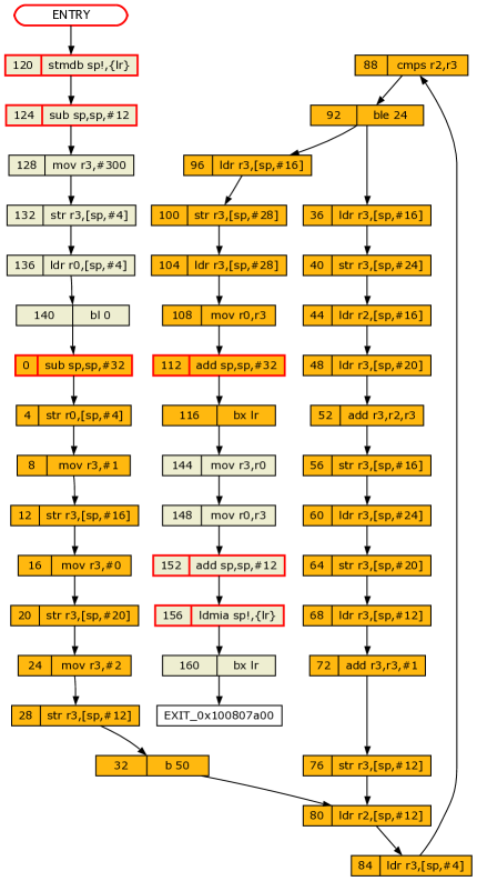
Figure 8: Second Unfolding of the CFG of $FIBO_{0}$.

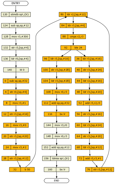
Figure 9: The Complete CFG of $FIBO_{0}$.

The computation of the possible values of sp described in Section 6.3 is actually performed when computing the CFG. When we have computed the final CFG we also have the possible values of register sp (at the stack reference node) and we can directly proceed to Step 2 (section 6.4) to compute a WCET-equivalent program.

The previous process always converge to the CFG of a program because we assume that the programs do not contain recursive calls (assumption (A4)). In the worst case, the slices we need to simulate in the iterative compuation are the full CFGs obtained at each step.

8 Hardware Model

In this section we present some features of the formal models (timed automata) of the hardware. The automata are given using the Uppaal syntax: initial locations are identified by double circles, guards are green, synchronization signals (channels) are light blue and assignments are dark blue. A C in a location means committed: when an automaton enters a committed location, it cannot be interrupted and proceeds immediately to one of the successors of this location (the guards determine the transitions that can be taken). The Uppaal models are available from http://www.irccyn.fr/franck/wcet.

8.1 Main Memory

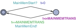
Figure 10: Main Memory TA

The main memory model is a very simple two-location automaton (Fig. 10). When a memory transfer is required, signal MainMemStart? is received and clock $t$ is reset. After a delay of MAINMEMTRANS the transfer is completed and signal MainMemEnd! is issued. Main memory transfers are triggered by either the instruction or data cache and accesses to main memory is serialized.

8.2 Caches

The model of the instruction cache is given in Fig. 11. The state of the cache contains an array ($64\times 8$ array) to record the addresses stored in the cache and whether a line is dirty or not.

The instruction cache is simpler than the data cache because no write can occur in this cache, so a line cannot be dirty. After the initialization of the cache (initial state of the cache by the function initCache()), the automaton is ready for receiving the signal CacheReadStart[num]?. This signal will be triggered by the fetch stage of the pipeline Fig. 12. The memory address to read is $m$. If $m$ is in the cache (function is_in(m) returns true), there is no need for a memory transfer and variable PMT (Pending Memory Transfers) is assigned $0$. Otherwise function insert(m) inserts $m$ in the cache and returns the number of memory transfers to be performed: for the instruction cache it is always $1$ because a line cannot be dirty (see Section 3) but for the data cache it can be either one or $2$ if a dirty line has to be saved from the cache. As soon as the memory transfer is completed (PMT=0) transition Hurry! is fired (it is urgent). Then, after CACHE_SPEED time units (value is $1$ for the our testbed) the read request completes and the signal CacheReadEnd[num]! is issued.

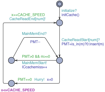
Figure 11: Instruction Cache

The data cache is a bit more involved (Fig. 13). For a read/hit operation it behaves almost like the instruction cache described above. For write operations, a write buffer (not given here) is used and moreover the timing depends on the type (load/store), addresses involved in the operation, and whether another write/read operation is already in progress (and to which line in the write buffer). We have tried to design an accurate model of the data cache: data cache operations are the major factor in the WCET for most of the programs and a faithful model is required to compute tight bounds. How the model of the data cache was built is described in Section 10.3.

8.3 Pipeline Model

The model of the pipeline is rather simple except the memory stage (M) which is a bit more complicated. The F stage automaton fetches the next instruction if no branch delay stall occurs (see Section 10.3). The function stall() of the F stage automaton determines whether such a stall should occur or not. If the next instruction can be fetched, it is fetched from the instruction cache CacheReadStart[INSTR_CACHE]! (this signal is urgent and synchronized with the instruction cache). When the fetch is completed the instruction is transferred to the next D stage, as soon as it is ready to be fed with a new instruction. The D stage, E stage and W stage are similar. Notice that the duration of an instruction may vary from one instruction to the other (e.g., long multiplication may take longer than additions) or because a conditional instruction is not executed: the actual duration is set when a new instruction arrives in the E stage (DUR_INSTR=dur()). A special signal prog_completed? is received from the program and marks the last instruction of the program. The program is completed when this last instruction flows out of the last stage (W) of the pipeline and this corresponds to reaching location DONE of the W stage.

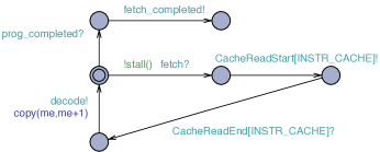
F Stage

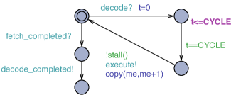
D stage

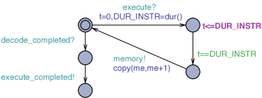
E Stage

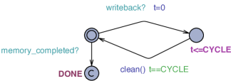
W Stage

Figure 12: Timed Automata for the Fetch, Decode, Execute and WriteBack Stages.

The automaton for the M stage is given in Fig. 13: when an instruction is performed and it is a memory transaction, it issues a sequence of read/write requests to the data cache.

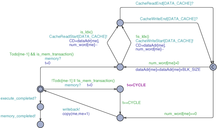
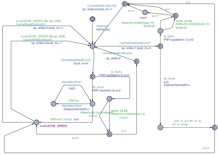
Figure 13: Memory Stage and Data Cache

9 Implementation

We have implemented the construction of the CFG (Section 7) and the computation of the WCET-equivalent program (Section 5). The architecture of our tool is given in Fig. 14. Together with a parser of ARM binary programs it comprises several thousand C++ lines of code. We have implemented very efficient versions of post-dominators algorithms [23, 18] and post dominance frontiers algorithms [13] as they are used intensively both in Compute CFG and Compute WCET-equiv. To obtain the binary program we use the GCC tool suite (gcc, objdump) from Codesourcery [12].

Figure 14: Tool Chain Overview

Our tool produces a bundle of files: a ready-to-analyse file containing the Uppaal timed automata models of the program $P^{\prime}$ and the hardware models $CFG(P^{\prime})$; a dot file with the graph of $P^{\prime}$ and a ready-to-compile C++ file that contains a simulator of the program $P^{\prime}$. This last file can be compiled and used to compute useful information like the ranges of registers. Notice that during the first phase Compute CFG we compute the range of the stack pointer and thus the tool can also be used as a stack analyser. To compute the WCET we check property R($K$) (Section 5.3) using Uppaal.

For the binary programs we have analysed, the time it takes to compute the output file from a binary program is negligible (less than a second). The automata of the programs of Table 1 and the dot graphs are available from http://www.irccyn.fr/franck/wcet.

10 Experiments

10.1 Methodology

The program $P$ to analyse is encapsulated in a template function: an example of use is given for program FIBO in Listing 3.

⬇

#define timerToCPUClockRatio 12

main ()

{

int result;

unsigned int start;

unsigned int stop;

start = timerGetValue(1);

result = fib(300);

stop = timerGetValue(1);

printf("fib(300):␣%d,␣time=%lu\n", result,

(stop-start)*timerToCPUClockRatio);

while (1);

}

Listing 3: Code snippet of instrumentation with FIBO

Given $P$, we let $t(P)$ be the encapsulated program. Measuring the execution time of $P$ consists in (1) reading a hardware timer (timerGetValue) into a $start$ variable, (2) calling the program $P$, and (3) reading the timer again into a $stop$ variable and (4) printing the difference $stop-start$. The function timerGetValue (assembly code) has been designed to read a hardware timer (See next paragraph).

The measurement error is is $+/-$$12$ processor cycles. The program $t(P)$ is compiled and linked. Running it on the ARM9 will print out the number of cycles taken by the program $P$: this figure is given in column “Measured WCET” in Table 1.

To faithfully compute the WCET of $P$ using our method, we take as input of our tool chain $t(P)$. $t(P)$ is transformed (using Compute CFG and Slice) into an Uppaal automaton as described in Section 9. In this automaton a dedicated clock GBL_CLK is reset when the instruction of $t(P)$ that reads the hardware timer flows out of the M stage (reading the timer in function timerGetValue is done using a load instruction). The final state of the automaton is reached when the second occurrence of the instruction that reads the timer flows out of the W stage. The computed WCET is given in column “Computed WCET” in in Table 1. Column “Uppaal” in Table 1 gives the time Uppaal takes to check the reachability property “Is it possible to reach a final states with GBL_CLK $\geq K+1$ ?” and this property is false and was true for $K$. In this case $K$ is the computed WCET.

10.2 Measuring Time on the Hardware

Measuring execution time on the hardware may be done by using an external device like an oscilloscope or by using one of the embedded hardware timers. In both cases, the program must be instrumented. In the first case, using a General Purpose I/O (GPIO) device, a signal is set to 1 at the start of the measure and to 0 at the end and the oscilloscope measures the time between the rising and the falling edge. In the second case, a free running timer is launched. It is read at the start and at the end of the measure. The difference of both values gives the execution time. This supposes the clock frequency of the hardware timer is close enough to the clock frequency of the processor to allow accurate measurements. By close enough we fix the measurement error to less than $+/-$$1\%$ of the measurement. So a hardware timer clock frequency two orders of magnitude lower than the processor clock frequency would be accurate enough if the program to measure executes in $\geq 10000$ cycles.

On the MC9328MXL the maximum available frequency for the hardware timers is $\frac{1}{12}th$ the processor clock frequency. So a program executing in $\geq 1200$ cycles may be accurately measured (less than $1\%$ error).

10.3 Tuning the Hardware Model

The ARM9TDMI Technical Reference Manual [2] gives pipeline timings according to the kind of instructions together with some examples of load delays and branch delays. However these timing information about the ARM920T processor and the MC9328MXL micro-controller are not enough to design accurate formal models of the hardware.

To overcome this, we have carefully crafted programs to stress particular features of the hardware and determine the precise timing of some sequences of instructions. The basis of this identification phase consists in measuring the difference in execution times of two variants of the same loop. The second variant contains a sequence of instructions for which we want a precise timing. The execution time difference between the two variants is the execution time of this sequence multiplied by the number of iterations. Using a large number of iterations minimizes the measurement error.

For memory accesses, variants may differ only by the memory alignment of data because timings may be different if a subsequent cache access is done in the same cache set or in a distinct cache set. And this can have a huge impact on the computed WCET if not modelled properly.

To remove the execution time of the measurement code, the loop is executed twice, one with 10000 turns and one with 20000 (for instance). The difference of execution time is the execution time of 10000 turns. The loop is dried run to copy it into the instruction cache.

Running a large set of special-purpose programs, we were able to refine the model of the data cache and obtain a rather precise formal model (see Fig. 13).

10.4 Test program example

This methodology allowed us to work out an undocumented behavior of the data cache. The loop in Listing 4 is executed 10000 times and 20000 times and the difference is 70000 cycles. This result is consistent with the timing of the instructions found in [2] since the instructions in the loop take 7 cycles to execute (execution time of each instruction is given as comment in listing 4).

⬇

.global ld_follow_st

ld_follow_st:

ldr r2,[r1,#0] @ preload both addresses

ldr r2,[r1,#16] @ in the data cache

ld_follow_st_loop:

str r2,[r1,#0] @ 1 cycle

ldr r2,[r1,#16] @ 1 cycle

sub r0,r0,#1 @ 1 cycle

cmp r0,#0 @ 1 cycle

bgt ld_follow_st_loop @ 3 cycles

bx lr

Listing 4: Data cache timing behavior test

However when the argument passed in r1 (the base address used to do the store and the load) is offset by 16 bytes, the execution time is 80000 cycles because the instructions in the loop take 1 extra cycle to execute.

The data cache has 64 sets and 32 bytes per line. So, the index is located in bits 10 to 5 of the address. In the first case, with $[\![r_{1}]\!]=0x8004d94$ and $[\![r_{1}]\!]+16=0x8004da4$, the indexes are different. In the second case, with $[\![r_{1}]\!]=0x8004da4$ and $[\![r_{1}]\!]+16=0x8004db4$, the indexes are equal. So, after a store in a set, an access to the same set incurs a 1 cycle stall.

10.5 Experiments on Benchmark Programs

The results we have obtained on some benchmark programs from Mälardalen University [19] are reported in Table 1. The programs we have analysed are available from http://www.irccyn.fr/franck/wcet: we have archived the C source program, the (de-assembled) encapsulated binary program (.arm file), the Uppaal model (and property) and the dot graph. We have not given the time it takes to do the slicing because it is less than a second. Regarding the benchmarks themselves, we point out that:

• the difficulty of measuring the WCET is not related to the size of the program; some programs are huge but contain a few paths, others are very compact but have a huge number of paths.

• they are designed to be representative of the difficulties encountered when computing WCET: for instance janne-complex contains two loops and the number of iterations of the inner loop depends on the current value of the counter of the outer loop (in a non regular way).

• we have experimented on different compiled versions of the same program (options O0, O1, O2) because the binary code produced stresses different parts of the hardware.

• we have checked various cases of the same programs with different initial stack pointer alignment, …

• we have multiplied the number of iterations of the benchmarks (e.g., we compute the execution time of $Fib(300)$); this way a modelling error (e.g., that adds $1$ cycle per iteration) is revealed and will incur a huge over-approximation.

In this sense the programs we have experimented on should not be considered too easy.

The results in Table 1 are divided into three main sections:

• Single-Path programs. The results of this section show that the abstract models (program and hardware) we have designed are adequate for obtaining tight bounds for the WCET. Even for janne-complex and its intriguing inner loop counts that depend on the outer loop counter, the maximum error is $3.2\%$. This also validates the accuracy of the program model we have computed (using slicing and no loop unrolling nor maximum loop bounds).

• Single-Path programs with data dependent instruction durations. Instructions like MUL/MLA can take between $3$ to $6$ cycles in the E stage (and SMULL $4$ to $7$). This section highlights one of the advantages of the timed automata models of the hardware. Indeed, in the timed automaton of the E stage (Fig. 12), we can replace the guard t==DURATION with MINDUR<= t <= MAXDUR and (add the assignments to MINDUR and MAXDUR). With this new E stage, we compute an interval for the WCET. Notice that this model is robust against timing anomalies because we explore the state space without any assumption like “always the shortest duration” or “always the largest duration”; the duration of the instruction is picked non-deterministically in [MINDUR,MAXDUR] every time the transition is taken. This explains the difference between the computed and the measured WCETs because in the measured WCET the worst-case duration for the MUL/MLA/SMULL instructions is never encountered. In this case, column $\frac{(C-M)}{M}$ of Table 1 does not represent the over-approximation of the computed WCET but rather the under-approximation of the measured WCET with the chosen input data.

• Multiple-path programs. These programs contain some branching that are input data dependent. The measured WCET is the execution time (on the hardware) obtained with input data that are supposed to produce the WCET. The computed WCET result considers all the possible input data. For bs-O0,O1,O2 the WCET is very small and measurement errors are more than $1\%$ (see Section 10.2). Program cnt starts with the initialization of a $10\times 10$ matrix. In cnt-O2, the compiler unrolls the initialization loop to a list of 100 consecutive store instructions. So cnt-O2 stresses the write buffer and we have to take into account the fact that the Write Buffer may be full. In this case, the data cache has to wait to make a write until the write buffer is not full.

Compared to existing methods and results our method has several advantages:

• computation of the CFG and of the reduced program automaton is fully automated (no loop bounds annotation needed);

• we use concrete caches and a detailed models of the hardware;

• the model of the hardware can be tuned easily (e.g., durations of instructions can be an interval instead of a fixed value); as emphasised in [10], changes in the processor speed can also be modelled easily (using a timed automaton that sets the processor speed). This enables us to compute WCET with power related constraints. Another advantage is that changing the processor (e.g., ARM7) requires only to change the pipeline automata.

• we compare the computed results to actual execution times using a rigorous protocol. The relative error in the computed results can be assessed and the results show that our method and models give very tight bounds.

Program	loc†	UPPAAL Time/States Explored¶	Computed WCET (C)	Measured WCET (M)	$\frac{(C-M)}{M}\times 100$	Abs§
Single-Path Programs
fib-O0	74	1.74s/74181	8098	8064	0.42%	47/131
fib-O1	74	0.61s/22332	2597	2544	2.0%	18/72
fib-O2	74	0.3s/9710	1209	1164	3.8%	22/71
janne-complex-O0∗	65	1.15s/38014	4264	4164	2.4%	78/173
janne-complex-O1∗	65	0.48s/14600	1715	1680	2.0%	30/89
janne-complex-O2∗	65	0.46s/13004	1557	1536	1.3%	32/78
fdct-O1	238	1.67s/60418	4245	4092	3.7%	100/363
fdct-O2	238	3.24s/55285	19231	18984	1.3%	166/3543
Single-Path Programs‡ with MUL/MLA/SMULL instructions (instructions durations depend on data)
fdct-O0	238	2.41s/85007	[11242,11800]	11448	3.0%	253/831
matmult-O0∗	162	5m9s/10531230	[502850,529250]	[511584,528684]	0.1%	158/314
matmult-O1∗	162	1m32s/1122527	[130001,156402]	[127356,153000]	2.2%	71/172
matmult-O2∗	162	43.78s/1780548	[122046,148299]	[116844,140664]	5.4%	75/288
jfdcint-O0	374	2.79s/100784	[12699,12699]	12588	0.8%	159/792
jfdcint-O1	374	1.02s/35518	[4897,4899]	4668	7.0%	25/325
jfdcint-O2	374	5.38s/175661	[16746,16938]	16380	3.4%	56/2512
Multiple-Path Programs
bs-O0	174	42.6s/1421474	1068	1056	1.1%	75/151
bs-O1	174	28s/1214673	738	720	2.5%	28/82
bs-O2	174	15s/655870	628	600	4.6%	28/65
cnt-O0∗	115	2.3s/76238	9028	8836	2.1%	99/235
cnt-O1∗	115	1s/27279	4123	3996	3.1%	42/129
cnt-O2∗	115	0.5s/11540	3065	2928	4.6%	39/263
insertsort-O0∗	91	10m35s/24250737	3133	3108	0.8%	79/175
insertsort-O1∗	91	7m2s/11455293	1533	1500	2.2%	40/115
insertsort-O2∗	91	11.5s/387292	1371	1344	2.0%	43/108
ns-O0∗	497	83.4s/3064315	30968	30732	0.8%	132/215
ns-O1∗	497	11.3s/368719	11701	11568	1.1%	61/124
ns-O2∗	497	29s/1030746	7343	7236	1.4%	566/863

 

^†lines of code in the C source file

^‡ $\frac{(C-M)}{M}\times 100$ computed using the upper bound for $C$ (see Section 10.5).

^§Non Abstracted instructions/Instructions

^∗Program selected for the WCET Challenge 2006

^¶Time in min/seconds on Intel Dual Core i3 3.2Ghz 8GB RAM

Table 1: Results. file-ox indicates that file was compiled using gcc -ox (optimization option).

11 Conclusion and Future Work

In this paper we have presented a framework based on program slicing and model-checking to compute WCET for programs running on architectures featuring pipelining and caching. We have exemplified the method by providing formal models of the ARM920T. Moreover we have compared the computed results with actual execution times on the real hardware. Our method is modular and altering the model of the hardware can be done easily using the timed automata models and the CFG is computed automatically.

In some cases there are a huge number of paths to be explored and there is no hope that an exhaustive search will compute any result in a life-time. Examples of such programs are multiple-path programs (e.g., program binary sort) with a lot of input data dependent branchings. To overcome this problem we are developing a branch and bound techniques. We are also currently extending the framework to handle:

• generation of traces: Uppaal can generate a witness symbolic trace of a path yielding the WCET. From this symbolic trace, we want to compute initial values of the input data that produce this trace. This can be achieved using techniques similar to Counter Example Guided Abstraction Refinement (CEGAR) [11].

• co-processor calls. This can be achieved by adding a timed automaton model of the co-processor.

• for some programs like OS kernels, interrupts can be generated and trigger interrupt handlers. Computing the WCET in this case is not easy as it requires a model of the interrupts arrivals e.g., “the interval between two interrupts of type $i$ is at least $t$ time units”. We can model interrupts arrivals using timed automata.

Acknowledgements.

The authors wish to thank Tim Bourke for the careful proof-reading of the paper and many helpful comments.

References

- [1] Armadeus systems.
- [2] ARM9TDMI Technical Reference Manual. ARM Limited, 2000.
- [3] Application Binary Interface for the ARM Architecture. ARM Limited, 2009.
- [4] AbsInt Angewandte Informatik. aiT Worst-Case Execution Time Analyzers. http://www.absint.com/ait/.
- [5] R. Alur and D. Dill. A theory of timed automata. Theoretical Computer Science, 126(2):183–235, 1994.
- [6] ARM Limited. Application Note 93 – Benchmarking with ARMulator. http://infocenter.arm.com/help/topic/com.arm.doc.dai0093a/DAI0093A_benchmarking_appsnote.pdf.
- [7] Clément Ballabriga, Hugues Cassé, Christine Rochange, and Pascal Sainrat. Otawa: An open toolbox for adaptive wcet analysis. In Sang Lyul Min, Robert G. Pettit IV, Peter P. Puschner, and Theo Ungerer, editors, Software Technologies for Embedded and Ubiquitous Systems (SEUS) - 8th IFIP WG 10.2 International Workshop, SEUS 2010, Waidhofen/Ybbs, Austria, October 13-15, 2010. Proceedings, volume 6399 of LNCS, pages 35–46. Springer, 2010.
- [8] Gerd Behrmann, Alexandre David, Kim Guldstrand Larsen, John Håkansson, Paul Pettersson, Wang Yi, and Martijn Hendriks. Uppaal 4.0. In QEST, pages 125–126. IEEE Computer Society, 2006.
- [9] G. Bernat, A. Colin, and S. M. Petters. pWCET a Toolset for automatic Worst-Case Execution Time Analysis of Real-Time Embedded Programs. In Proceedings of the 3rd Int. Workshop on WCET Analysis, Workshop of the Euromicro Conference on Real-Time Systems, Porto, Portugal, 2003.
- [10] Franck Cassez. Timed Games for Computing WCET for Pipelined Processors with Caches. In 11th Int. Conf. on Application of Concurrency to System Design (ACSD’11). IEEE Comp. Soc., June 2011. forthcoming.
- [11] Edmund M. Clarke, Orna Grumberg, Somesh Jha, Yuan Lu, and Helmut Veith. Counterexample-guided abstraction refinement for symbolic model checking. J. ACM, 50(5):752–794, 2003.
- [12] Codesourcery. Web site. http://www.codesourcery.com/.
- [13] Keith D. Cooper, Timothy J. Harvey, and Ken Kennedy. A Simple, Fast Dominance Algorithm. Software – Practice and Experience, 4:1–10, 2001.
- [14] Andreas E. Dalsgaard, Mads Chr. Olesen, Martin Toft, René Rydhof Hansen, and Kim Guldstrand Larsen. Metamoc: Modular execution time analysis using model checking. In Björn Lisper, editor, WCET, volume 15 of OASICS, pages 113–123. Schloss Dagstuhl - Leibniz-Zentrum fuer Informatik, Germany, 2010.
- [15] Andreas Engelbredt Dalsgaard, Mads Christian Olesen, and Martin Toft. Modular execution time analysis using model checking. Master’s thesis, Department of Computer Science, Aalborg University, Denmark, 2009.
- [16] Jakob Engblom, Andreas Ermedahl, Mikael Nolin, Jan Gustafsson, and Hans Hansson. Worst-case execution-time analysis for embedded real-time systems. Journal on Software Tools for Technology Transfer (STTT), 4(4):437–455, October 2003.
- [17] Christian Ferdinand, Reinhold Heckmann, and Reinhard Wilhelm. Analyzing the worst-case execution time by abstract interpretation of executable code. In Manfred Broy, Ingolf H. Krüger, and Michael Meisinger, editors, ASWSD, volume 4147 of LNCS, pages 1–14. Springer, 2004.
- [18] Loukas Georgiadis, Robert Endre Tarjan, and Renato Fonseca F. Werneck. Finding dominators in practice. J. Graph Algorithms Appl., 10(1):69–94, 2006.
- [19] Jan Gustafsson, Adam Betts, Andreas Ermedahl, and Björn Lisper. The Mälardalen WCET benchmarks – past, present and future. pages 137–147, Brussels, Belgium, July 2010. OCG.
- [20] Niklas Holsti, Jan Gustafsson, Guillem Bernat, Clément Ballabriga, Armelle Bonenfant, Roman Bourgade, Hugues Cassé, Daniel Cordes, Albrecht Kadlec, Raimund Kirner, Jens Knoop, Paul Lokuciejewski, Nicholas Merriam, Marianne De Michiel, Adrian Prantl, Bernhard Rieder, Christine Rochange, Pascal Sainrat, and Markus Schordan. Wcet 2008 - report from the tool challenge 2008. In Proceedings of the 8th Intl. Workshop on Worst-Case Execution Time (WCET) Analysis (WCET’08), Prague, Czech Republic, July 2008.
- [21] Benedikt Huber and Martin Schoeberl. Comparison of Implicit Path Enumeration and Model Checking Based WCET Analysis. In Proceedings of the 9th Intl. Workshop on Worst-Case Execution Time (WCET) Analysis (WCET’09), Dublin, Ireland, July 2009.
- [22] K. G. Larsen, P. Pettersson, and W. Yi. Uppaal in a Nutshell. Journal of Software Tools for Technology Transfer (STTT), 1(1-2):134–152, 1997.
- [23] Thomas Lengauer and Robert Endre Tarjan. A fast algorithm for finding dominators in a flowgraph. ACM Trans. Program. Lang. Syst., 1(1):121–141, 1979.
- [24] Xianfeng Li, Yun Liang, Tulika Mitra, and Abhik Roychoudhury. Chronos: A Timing Analyzer for Embedded Software. Science of Computer Programming, 69(1–3), 2007. Special Issue on Experimental Software and Toolkit.
- [25] Mingsong Lv, Wang Yi, Nan Guan, and Ge Yu. Combining Abstract Interpretation with Model Checking for Timing Analysis of Multicore Software. In 31st IEEE Real-Time Systems Symposium (RTSS’2010), pages 339–349. IEEE Comp. Soc., 2010.
- [26] Alexander Metzner. Why Model Checking Can Improve WCET Analysis. In Rajeev Alur and Doron Peled, editors, CAV, volume 3114 of LNCS, pages 334–347. Springer, 2004.
- [27] A. Prantl, M. Schordan, and J. Knoop. TuBound - A Conceptually New Tool for WCET Analysis. In Proceedings of the 8th Intl. Workshop on Worst-Case Execution Time (WCET) Analysis (WCET’08), Prague, Czech Republic, July 2008.
- [28] Rapita Systems Ltd. Rapita Systems for timing analysis of real-time embedded systems. http://www.rapitasystems.com/.
- [29] B. Rieder, P. Puschner, and I. Wenzel. Using Model Checking to Derive Loop Bounds of General Loops within ANSI-C Applications for Measurement Based WCET Analysis. In Proc. of the 6th Int. Workshop on Intelligent Solutions in Embedded Systems (WISES’08), Regensburg, Germany, 2008.
- [30] Tidorum Ltd. Bound-T time and stack analyser. http://www.tidorum.fi/bound-t/.
- [31] F. Tip. A survey of program slicing techniques. JOURNAL OF PROGRAMMING LANGUAGES, 3:121–189, 1995.
- [32] Mark Weiser. Program slicing. IEEE Trans. Software Eng., 10(4):352–357, 1984.
- [33] Reinhard Wilhelm, Jakob Engblom, Andreas Ermedahl, Niklas Holsti, Stephan Thesing, David B. Whalley, Guillem Bernat, Christian Ferdinand, Reinhold Heckmann, Tulika Mitra, Frank Mueller, Isabelle Puaut, Peter P. Puschner, Jan Staschulat, and Per Stenström. The Worst-Case Execution-Time Problem - Overview of Methods and Survey of Tools. ACM Trans. Embedded Comput. Syst., 7(3), 2008.