The Sloan Great Wall. Morphology and galaxy content

Abstract

We present the results of the study of the morphology and galaxy content of the Sloan Great Wall (SGW), the richest galaxy system in the nearby Universe. We use the luminosity density field to determine superclusters in the SGW, and the 4th Minkowski functional $V_{3}$ and the morphological signature (the $K_{1}$-$K_{2}$ shapefinders curve) to show the different morphologies of the SGW, from a single filament to a multibranching, clumpy planar system. We show that the richest supercluster in the SGW, SCl 126 and especially its core resemble a very rich filament, while another rich supercluster in the SGW, SCl 111, resembles a “multispider”—an assembly of high density regions connected by chains of galaxies. We study the substructure of individual galaxy populations determined by their color in these superclusters using Minkowski functionals and find that in the high density core of the SGW the clumpiness of red and blue galaxies is similar, but in the outskirts of superclusters the distribution of red galaxies is more clumpy than that of blue galaxies. At intermediate densities, the systems of blue galaxies have tunnels through them. We assess the statistical significance of our results using the halo model and smoothed bootstrap.

We study the galaxy content and the properties of groups of galaxies in two richest superclusters of the SGW, paying special attention to bright red galaxies (BRGs) and to the first ranked galaxies in SGW groups. The BRGs are the nearby LRGs, they are mostly bright and red and typically reside in groups (several groups host 5 or more BRGs). About 1/3 of BRGs are spirals. The scatter of colors of elliptical BRGs is smaller than that of spiral BRGs. About half of BRGs and of first ranked galaxies in groups have large peculiar velocities. Groups with elliptical BRGs as their first ranked galaxies populate superclusters more uniformly than the groups, which have a spiral BRG as its first ranked galaxy.

The galaxy and group content of the core of the supercluster SCl 126 shows several differences in comparison with the outskirts of this supercluster and with the supercluster SCl 111. Here groups with BRGs are richer and have larger velocity dispersions than groups with BRGs in the outskirts of this supercluster and in SCl 111. The fraction of those BRGs which do not belong to any group is the smallest here. In the core of the supercluster SCl 126 the fraction of red galaxies is larger than in the outskirts of this supercluster or in the supercluster SCl 111. Here the peculiar velocities of of the first ranked galaxies are larger than in the outskirts of this supercluster or in the supercluster SCl 111 and the peculiar velocities of elliptical BRGs are larger than those of spiral BRGs, while in the outskirts of this supercluster and in the supercluster SCl 111 the peculiar velocities of spiral BRGs are larger than those of elliptical BRGs.

All that suggests that the formation history and evolution of individual neighbour superclusters in the SGW has been different, and the SGW is not a genuine physical structure but an assembly of very rich galaxy systems.

1. Introduction

Observations and simulations of the large scale structure of the Universe have revealed the presence of a supercluster-void network—a network of galaxies, groups and clusters of galaxies connected by filaments (Joeveer et al., 1978; Gregory & Thompson, 1978; Zeldovich et al., 1982; Einasto et al., 1984; de Lapparent et al., 1986). The formation of a web of galaxies and systems of galaxies is predicted in any physically motivated theories of the formation of the structure in the Universe (Bond et al., 1996). Bond et al. (2010b) emphasize that if we want to understand the patterns of the large scale structure (cosmic web) we need to know how to quantify them. One approach for that is the study of the morphology of systems of galaxies.

Galaxies and galaxy systems form due to initial density perturbations of different scale. Perturbations of a scale of about 100 $h^{-1}$ Mpc give rise to the largest superclusters. The largest and richest superclusters which may contain several tens of rich (Abell) clusters are the largest coherent systems in the Universe with characteristic dimensions of up to 100 $h^{-1}$ Mpc. At large scales dynamical evolution takes place at a slower rate and the richest superclusters have retained the memory of the initial conditions of their formation, and of the early evolution of structure (Kofman et al., 1987).

Rich superclusters had to form earlier than smaller superclusters; they are the sites of early star and galaxy formation (e.g. Mobasher et al., 2005), and the first places where systems of galaxies form (e.g. Venemans et al., 2004; Ouchi et al., 2005). Observations already have revealed superclusters at high redshifts (Nakata et al., 2005; Swinbank et al., 2007; Gal et al., 2008; Tanaka et al., 2009).

Early supercluster catalogues have been compiled using the data on clusters of galaxies (Zucca et al., 1993; Einasto et al., 1994; Kalinkov & Kuneva, 1995; Einasto et al., 2001). The advent of the deep surveys of galaxies as (2dFGRS and SDSS, see Colless et al., 2003; Abazajian et al., 2009) started a new era in the studies of the large scale structure of the Universe, where systems of galaxies can be studied in a detail impossible before. Using these data, a number of supercluster catalogues have been compiled (Basilakos, 2003; Einasto et al., 2003b, a; Erdoğdu et al., 2004, and references therein).

Superclusters are important traces of the baryonic matter in the Universe (Génova-Santos et al., 2005; Padilla-Torres et al., 2009). Observations have revealed the presence of warm-hot diffuse gas (WHIM) in the Sculptor supercluster and nearby Sculptor Wall associated with the inter-cluster galaxy distribution in these superclusters (Zappacosta et al., 2005; Buote et al., 2009, and references therein), often referred to as the “missing baryons”. Detailed structural and spatial information on nearby superclusters could help the targeted search for WHIM.

Gravitational lensing analysis of supercluster structure can be used to reconstruct the distribution of dark matter in superclusters as has been done for the supercluster A901/902 (Heymans et al., 2008).

Rich superclusters contain a variety of evolutionary phases of galaxy systems and their environment is suitable for studies of the properties of cosmic structures and the properties of galaxies therein in a wide range of densities in a consistent way, helping us to understand the role of environment in the evolution of galaxies and groups of galaxies. A number of studies have already shown that the supercluster environment affects the properties of galaxies, groups and clusters located there (Einasto et al., 2003c; Plionis, 2004; Wolf et al., 2005; Haines et al., 2006; Einasto et al., 2007c; Porter et al., 2008; Fleenor & Johnston-Hollitt, 2009; Tempel et al., 2009; Lietzen et al., 2009).

A comparison of the properties of rich and poor superclusters have revealed a number of differences between them. The mean and maximum densities of galaxies in rich superclusters are larger than in poor superclusters. Rich superclusters are more asymmetrical than poor superclusters (Einasto et al., 2007b). Rich superclusters contain high density cores (Einasto et al., 2007c, 2008). Small et al. (1998) showed in a study of the Corona Borealis supercluster that the core of this supercluster may be collapsing. The fraction of X-ray clusters in rich superclusters is larger than in poor superclusters (Einasto et al., 2001, hereafter E01). The core regions of the richest superclusters may contain merging X-ray clusters (Bardelli et al., 2000; Rose et al., 2002). The morphology of rich and poor superclusters is different—poor superclusters (as an example we can use the Local Supercluster) resemble a “spider”–a rich cluster with surrounding filaments while rich superclusters resemble a “multispider”—several high density regions (cores) connected by filaments (Einasto et al., 2007d).

The extreme cases of observed objects usually provide the most stringent tests for theories; this motivates the need for a detailed understanding of the richest superclusters. So far, even their existence is not well explained by the main contemporary structure modeling tool, numerical simulations: while the masses of the richest simulated superclusters are similar to those of the richest observed superclusters (Einasto et al., 2007d, b; Araya-Melo et al., 2009a), the number density of the richest superclusters in simulations is about ten times smaller than the number density of observed superclusters (Einasto et al., 2006). Yamila Yaryura et al. (2010) reached similar conclusions analysing rich systems in the 2dFGRS data. Bardelli (2004) mentioned that the mass of the Shapley supercluster is very rarely reproduced in the $\lambda$CDM model. It has even been argued that the existence of very large superclusters contradicts with the concept of a homogeneous Universe at large scales (Sylos Labini et al., 2009).

The richest relatively close superclusters, which have been studied in detail, are the Shapley Supercluster (Proust et al., 2006, and references therein) and the Horologium–Reticulum Supercluster (Rose et al., 2002; Fleenor et al., 2005, 2006; Fleenor & Johnston-Hollitt, 2009).

Among the richest known galaxy systems, the Sloan Great Wall (SGW) deserves a special attention. The SGW is the richest and largest system of galaxies observed in the nearby Universe so far (Vogeley et al., 2004; Gott et al., 2005; Nichol et al., 2006). The SGW consists of several superclusters of galaxies; the richest of them is the supercluster SCl 126 from the E01 catalogue. The core of the supercluster SCl 126 contains many rich clusters of galaxies, with X-ray clusters among them (Belsole et al., 2004; Einasto et al., 2007d). Interestingly, the SGW has not been studied in detail yet, but already now we know that numerical simulations have been unable to reproduce several properties of the SGW. The SGW affects the measurements of the genus and Minkowski functionals of the SDSS and 2dF redshift surveys (Park et al., 2005; Saar et al., 2007; Gott et al., 2008), causing a “meatball” shift of the genus curve (a cluster-dominated morphology) of these surveys compared with the genus curve from simulations. Croton et al. (2004); Nichol et al. (2006) showed that the higher order moments of the correlation function of the SDSS and 2dFGRS are sensitive to the presence of the SGW and cause a disagreement between higher order correlation functions in observations and in numerical simulations. (Interestingly, the observed correlations can be explained by non-Gaussian initial density fields, Gaztanaga & Maehoenen, 1996). Nichol et al. (2006) mentions also that this disagreement may be due to the unusual morphology of the SGW. As we already mentioned, cosmological simulations have been unable to reproduce very rich extended systems as the SGW (Sylos Labini et al., 2009).

Einasto et al. (2007d, 2008) showed that the morphology of the richest supercluster in the SGW, the supercluster SCl 126 is unusual—it resembles a very rich filament with a high density core, while other rich superclusters (both observed and simulated), the morphology of which we have studied, can in general be called “multispiders”—several high-density clusters are connected by lower density filaments. This is another disagreement between the simulations and one supercluster in the SGW.

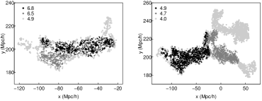
Figure 1.— Distribution of galaxies in the Sloan Great Wall region. The coordinates x and y are in Mpc/$h$ (their definition is given in the Appendix, Eq. A.2). The left panel shows the SCl 126 region, the right panel—a wider region with nearby superclusters. The surrounding region is shown in Fig. 2. The relative luminosity density $D$ (normalized by the mean density) limits are as follows: left panel: black: $D\geq 6.8$, dark grey: $D\geq 6.5$, light grey: $D\geq 4.9$. Right panel: black: $D\geq 4.9$ (the same as the lightest level in the left panel), dark grey: $D\geq 4.7$, light grey: $D\geq 4.0$.

All this shows the importance of the studies of the morphology of superclusters. Information about the complex patterns of the large scale structure (the cosmic web) gets lost when we use, for example, correlation functions to study the clustering of galaxies (see Coles, 2009, for details and references) and also van de Weygaert & Schaap (2009) for further reading about cosmic patterns). As we saw above, information about the morphology of the superclusters is useful when we interpret the results of the measurements of the correlation function.

Morphology of superclusters can be used as one of the tests to compare superclusters from observations and simulations. Basilakos (2003) used supercluster shape as a cosmological probe to compare observed superclusters with those from simulations and showed that in this respect the $\Lambda$CDM model is in a better agreement with observations than the $\tau$CDM model.

In the present paper we study the morphology of the full SGW and of individual superclusters in the SGW with the aim to quantify the morphology of the SGW and to determine whether all superclusters in the SGW (and the full SGW) have peculiar morphologies not found in simulated superclusters. This study may help to answer the question whether the SGW is a genuine physical structure (van de Weygaert & Schaap, 2009). We use Minkowski functionals to compare substructure of superclusters in the SGW defined by different galaxy populations. We also compare the galaxy and group content of individual superclusters in the SGW with the goal to search for possible differences between superclusters in this aspect.

First we delineate the superclusters in the SGW region, calculating the luminosity density field of galaxies from the SDSS DR7. We study the morphology of the SGW and individual superclusters in it, using Minkowski functionals and shapefinders. Next we study the morphology of these superclusters as determined by individual galaxy populations—this analysis gives us information about the substructure of superclusters. We define galaxy populations by their color, and add a separate population of bright red galaxies (BRGs). We assess the statistical significance of our results using Monte Carlo simulations.

Then we compare the galaxy and group content of the two richest superclusters in the SGW and search for differences between these superclusters. We compare the properties of groups in them, study the group membership of BRGs, and analyze colors and morphological types of BRGs and the distribution of groups with different morphological types of BRGs in superclusters. We compare the peculiar velocities of elliptical and spiral BRGs and the first ranked galaxies in groups. The peculiar velocities of the first ranked galaxies in groups can be used as indicators of the dynamical state of groups and clusters (Coziol et al., 2009). Comparison of the peculiar velocities of the first ranked galaxies in groups in different superclusters of the SGW gives us information about the dynamical state of groups.

The BRGs satisfy the criteria for nearby ($z<0.15$, cut I) LRGs (Eisenstein et al., 2001). Eisenstein et al. (2001) warn that the sample of nearby LRGs may be contaminated by galaxies of lower luminosity not suitable for a volume-limited sample, thus we call them BRGs (the name could be misleading, as the LRGs were first called thus; unfortunately, we have not found a better name). These galaxies can also be spirals; we will carry out their morphological classification. Understanding the spatial distribution and properties of the LRGs is of great cosmological importance, and our study of their nearby population (BRGs) will help to specify their properties.

2. Data

2.1. Galaxies, groups and superclusters

Table 1Superclusters in the region of the Sloan Great Wall.

(1)	(2)	(3)	(4)	(5)	(6)	(7)	(8)	(9)	(10)
Nr.	ID	ID	$N_{\mbox{gal}}$	$N_{\mbox{gr}}$	$d_{\mbox{peak}}$	$V$	$L_{\mbox{tot}}$	$D_{\mbox{peak}}$	Diam.
					Mpc/$h$	(Mpc/$h$)3	$10^{10}h^{-2}L_{\sun}$	¡dens¿	Mpc/$h$
1	111	184+003+007	1515	208	230.3	10565	1105.8	14.16	56.9
2	111	173+014+008	1334	190	242.0	10193	1050.8	12.31	50.3
3	126,136	202-001+008	3162	425	255.6	24558	2539.0	12.92	107.8
4	88	152-000+009	487	65	285.1	4666	453.5	9.81	39.0
5		187+008+008	711	73	267.4	4665	431.6	9.33	54.2
6		170+000+010	190	24	302.1	1841	171.0	8.55	20.1
7		175+005+009	348	51	291.0	3406	311.1	8.23	28.0
8	91	159+004+006	215	23	206.6	1108	98.3	7.61	15.4
9	91	168+002+007	387	34	227.7	1802	156.4	7.49	28.1
10		214+001+005	332	33	162.6	1086	94.2	7.22	19.5
11		189+003+008	468	70	254.1	2686	226.3	6.75	32.2
12		198+007+009	100	18	276.0	649	53.7	6.33	13.1
13	91	157+003+007	111	6	219.1	148	11.4	5.28	13.3

We used the MAIN galaxy sample and the SDSS-LRG sample from the 7th data release of the Sloan Digital Sky Survey (Adelman-McCarthy et al., 2008; Abazajian et al., 2009). From these data we chose a subsample of the SGW region: $150^{\circ}\leq R.A.\leq 220^{\circ}$, $-4^{\circ}\leq\delta\leq 8^{\circ}$, within the distance limits 150 $h^{-1}$ Mpc$\leq D_{com}\leq$ 300 $h^{-1}$ Mpc. This region fully covers the SGW and its surroundings, including poor superclusters, which connect the SGW with other nearby rich superclusters. In this region there are 27113 galaxies from the MAIN SDSS galaxy sample, and 3168 BRGs, which have been selected from the SDSS database; they are nearby ($z<0.15$) LRGs (Eisenstein et al., 2001) (cut I LRGs).

We found groups of galaxies on the basis of the MAIN galaxy sample, as described in detail in Tago et al. (2010), hereafter T10, and Tago et al. (2008). We corrected the redshifts of galaxies for the motion relative to the CMB and computed the co-moving distances (Martínez & Saar, 2002) of galaxies using the standard cosmological parameters: the Hubble parameter $H_{0}=100h\,$km sec^-1Mpc^-1, the matter density $\Omega_{m}=0.27$, and the dark energy density $\Omega_{\Lambda}=0.73$. Our SGW region sample contains about 4000 groups of galaxies.

In T10 groups of galaxies have been defined applying the Friends-of-Friends cluster analysis method introduced by Turner & Gott (1976); Zeldovich et al. (1982); Huchra & Geller (1982), and modified by us (Tago et al., 2008). In this algorithm galaxies are linked into systems using a variable linking length. By definition, a galaxy belongs to a group of galaxies if this galaxy has at least one group member galaxy closer than the linking length. To take into account selection effects when constructing a group catalogue from a flux-limited sample, T10 calibrated the scaling of the linking length with distance, using nearby rich groups as a template. As a result, the maximum group sizes in the sky projection and the velocity dispersions of groups in our catalogue are similar at all distances.

The T10 group catalogue is available in electronic form at the CDS via anonymous ftp to cdsarc.u-strasbg.fr (130.79.128.5) or via http://cdsweb.u-strasbg.fr/cgi-bin/qcat?J/ A+A/514/A102.

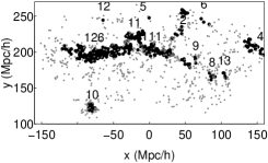
Figure 2.— Groups with at least four member galaxies in the Sloan Great Wall region (for the SGW proper see Fig. 1). Filled black circles show the groups in superclusters, and filled grey circles show those groups, which do not belong to superclusters. The numbers are the supercluster numbers in Table LABEL:tab:scldata (for the superclusters SCl 126 and SCl 111 we give the ID from the E01 catalogue, see text).

Next we calculated the luminosity density field of galaxies and found extended systems of galaxies (superclusters) in this density field. This procedure is described in more detail in Appendix A. Supercluster catalogue is described in detail in Liivamägi et al. (2010).

To search for systems (high density regions) in the distribution of galaxies and clusters of galaxies usually either the Friend-of-Friend algorithm or a density field approach is used. In the Friend-of-Friend method galaxies or clusters of galaxies are collected together so that each object has at least one neighbor closer than the linking length (a fixed distance). For small linking lengths all objects are isolated. When the linking length increases more and more objects are collected into systems, and as a result, the richnesses and lengths of systems increase. At a certain linking length systems join rapidly and form a system that may penetrate the whole volume under study—percolation occurs. Superclusters as the largest still relatively isolated systems are determined using a linking length smaller than the percolation length (for details we refer to Zucca et al., 1993; Einasto et al., 1994, 2001). When using the density field to select systems, we search for connected systems with the density higher than a certain threshold. When we decrease the density threshold, then, as with increasing linking length in the Friend-of-Friend method, more objects join the systems, and the richnesses and lengths of systems increase. At a certain threshold the systems percolate the sample volume. Again, supercluster catalogues are compiled using a density threshold higher than the percolation threshold (Einasto et al., 2003b, a; Erdoğdu et al., 2004; Einasto et al., 2007a). Erdoğdu et al. (2004) used a varying density threshold to determine superclusters using the 2dF data; for details we refer to their study. While the Friend-of-Friend method tends to find elongated systems (Einasto et al., 1984), the density field approach does not have such a bias.

Comparison of different catalogues of superclusters shows that rich superclusters can be identified in different ways, with similar parameters (e.g., the maximum length). For example, the supercluster SCl 126 has been identified in Einasto et al. (2003a) using the SDSS data and the density field (the supercluster N13 in the list), and has a length of 90$h^{-1}$ Mpc; in Einasto et al. (2003b) this supercluster is determined using the 2dF data, this is the supercluster SCl 152 in the list with the length of 112$h^{-1}$ Mpc. In Erdoğdu et al. (2004) list this supercluster is the supercluster SCNGP06.

In order to choose proper density levels to determine the SGW and the individual superclusters, which belong to the SGW, we compared the density field superclusters at a series of density levels (Fig. 1). We analyzed the systems of galaxies at each level, and examined the joining events, when we moved from higher density levels to lower ones. We will use the relative luminosity density $D$ here and below (normalized to the mean density in the SDSS sample volume). At a very high density level ($D=6.8$) only the highest density part of the SGW is seen. This can be identified with the core region of the supercluster SCl 126 in the E01 catalogue. We use this density level to define the core of this supercluster, and denote it as SCl 126c. As we decrease the density level, galaxies from the outskirts of the SCl 126 join the SGW. At the density level $D=4.9$ the richest two superclusters in the SGW (SCl 126 and SCl 111) still form separate systems. At a lower density level, $D=4.7$, these two superclusters join together to become one connected system, and several other superclusters also join this system. At a still lower density level ($D=4.0$) these superclusters, which border the voids around the SGW, join the SGW. Several poor superclusters, which form a low-density extension of the SGW, join the SGW at this level, too. We show in Fig. 1 the full SGW region and the surrounding superclusters at different density levels from $D=6.8$ to $D=4.0$.

We used the information about joining of superclusters to determine the SGW and the individual superclusters in the SGW as follows.

First, we used the density level $D=4.9$ to determine individual superclusters, which belong to the SGW. In Fig. 2 we show and mark all superclusters of galaxies in the SGW region. The data on these superclusters are presented in Table LABEL:tab:scldata.

The richest superclusters in the SGW are the superclusters SCl 126 and the supercluster SCl 111. The supercluster SCl 126 includes also the supercluster SCl 136 from the E01 catalogue. We note that the supercluster SCl 111 in the E01 catalogue actually corresponds to two superclusters in the SGW region, the first and second supercluster in Table LABEL:tab:scldata. In what follows we will call the first supercluster in this table SCl 111, as the second supercluster actually does not belong to the SGW (see Fig. 2). We will use the notation SCl 126c for the core region of the supercluster SCl 126, and the notation SCl 126o for the outskirts of this supercluster, defined by excluding the core SCl 126c from the whole supercluster SCl 126.

We use the density level $D=4.7$ to determine the whole SGW. This adds to the SGW also those poor superclusters, which form the low density extension of the SGW (superclusters 9, 8, and 13 in Table LABEL:tab:scldata, which all belong to the SCl 91 in the E01 catalogue). Thus, the highest density part of the SGW is the supercluster SCl 126 and the lowest density part is formed by poor superclusters, members of the supercluster SCl 91 in the E01 catalogue. In addition, we combine those galaxies, groups and poor superclusters in the volume defined at the start of this Section, which do not belong to the SGW, into a comparison sample and call it the field sample (denoted as F). Our SGW sample contains 6138 galaxies and 817 groups, 351 of which host BRGs. The field sample contains 20975 galaxies and 3020 groups; 1589 groups in the field have BRGs in them. In the SGW 83% of all BRGs belong to groups, in the field—68%.

2.2. Galaxy populations

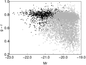
Figure 3.— The color-magnitude diagram of the SGW galaxies. Open circles – main sample galaxies, filled circles – BRGs.

In the present paper we use the $g-r$ colors of galaxies and their absolute magnitude in the $r$-band $M_{r}$. The absolute magnitudes of individual galaxies are computed using the the KCORRECT algorithm (Blanton et al., 2003a; Blanton & Roweis, 2007). We also accepted $M_{\odot}=4.53$ (in the $r$ photometric system). Evolution correction $e$ has been calibrated according to Blanton et al. (2003b). All of our magnitudes and colors correspond to the rest-frame at the redshift $z=0$. We note that our colors are found using the rest-frame Petrosian magnitudes, not the model magnitudes as done by Eisenstein et al. (2001), so there might be small differences in the colors.

Figure 4.— The distribution of the $g-r$ colors for galaxies in the SGW and in the field (F) (left panel), in the supercluster SCl 126 (core and outskirts, SCl 126c and SCl 126o) and SCl 111 (middle panel), and in the superclusters 9 and 11 (right panel, see Table LABEL:tab:scldata for supercluster ID). The color distributions were calculated for the absolute magnitude $M_{r}$ limit $M_{r0}\leq-19.25$. All distributions were calculated using the ’density’ command in the R statistical environment with the bandwidth 0.015. The numbers of galaxies in each sample are as follows: SGW—5925, field—18611, SCl 126c—1397, SCl 126o—1751, SCl 111—1419, SCl 09—355, and SCl 111—454 galaxies.

As said above, we will pay special attention to two populations of galaxies, the first-ranked galaxies of groups, and the BRGs (the galaxies that have the GALAXY_RED flag in the SDSS database). The BRGs are nearby ($z<0.15$, cut I) LRGs (Eisenstein et al., 2001) and are similar to the LRGs at higher redshifts. Nearby bright red galaxies do not form an approximately volume-limited population, but they are yet the most bright and the most red galaxies in the SGW region, as shown in Fig. 3.

BRGs have been selected using model magnitudes, but in our analysis we will use rest-frame Petrosian magnitudes for all galaxies including BRGs, for concordance.

For a small subsample of galaxies (the BRGs and the first-ranked galaxies in groups, Sect. 4) we determined also the morphological types of galaxies, using data from the SDSS visual database. We used pseudo true-color images and followed the classification, used in the Galaxy Zoo project (Lintott et al., 2008)—elliptical galaxies are of type 1, spiral galaxies of type 4, those galaxies which show signs of merging or other disturbancies, are of type 6. Types 2 and 3 denote clockwise and anti-clockwise spiral galaxies, for which spiral arms are visible. Fainter galaxies, for which the morphological type is difficult to determine, are of type 5. The use of pseudo-color images may, in principle, intruduce a bias toward blue-looking galaxies to be classified as spirals and red-looking galaxies—as ellipticals. We tried to avoid this: several people classified galaxies independently. Later comparison showed that in most cases these independent classifications coincided. Our sample of the BRGs and the 1st ranked galaxies consists of quite bright galaxies, so it was possible to determine their morphological type reliably.

Eisenstein et al. (2001) warn that the sample of nearby LRGs may be contaminated by galaxies of lower luminosity not suitable for the use of nearby BRGs as a volume-limited sample. Nearby BRGs may also be of late type and/or, as shows Fig. 3, some of them may have blue $g-r$ colors. Later we will compare the colors and morphological types of BRGs in color-magnitude diagrams to check for probable presence of blue, late type galaxies in our sample of BRGs.

Images of individual galaxies, which we used for morphological classification, can be found at {http://www.aai.ee/$∼$maret/SGWmorph.html}.

We divide the galaxies into the red and blue populations, using the color limit $g-r\geq 0.7$ (we call these galaxies red). We use volume limited samples with the $r$-band magnitude limit $M_{r}=-19.25$. We show in Fig. 4 the distributions of the $g-r$ colors of galaxies in the whole SGW and in the individual superclusters in the SGW. The numbers of galaxies in each sample are given in caption. Comparison with the numbers of galaxies in superclusters in Table LABEL:tab:scldata shows that actually all samples are almost volume limited—the selection effects were taken into account correctly when we calculated the luminosity density field.

In the present paper all the distributions (probability densities) were calculated within the R environment using the ’density’ command in the ’stats’ package (Ihaka & Gentleman, 1996), http://www.r-project.org. The ’density’ function chooses the optimal bin width minimizing the MISE (mean integral standard error) of the estimate. This package does not provide the customary error limits (local error estimates), but the usual Poisson errors do not describe these, also (we explained this in more detail in Einasto et al., 2008). We compare the density distributions using the full data (i.e. the integral distributions) and statistical tests, as the Kolmogorov-Smirnov test, throughout the paper.

Fig. 4 shows that in the whole SGW the fraction of red galaxies is larger than in the field, an evidence of the large-scale morphological segregation (Einasto et al., 2007c). In the SGW, 65% of galaxies are red, in the field—51%. In addition, there are relatively more red galaxies in the core of the supercluster SCl 126 (SCl 126c) than in other superclusters (Table LABEL:tab:sclgal). This agrees with earlier findings by Einasto et al. (2007d, c). We used the Kolmogorov-Smirnov test to estimate the statistical significance of the differences between the colors of galaxies in different superclusters. This test showed that the differences between the colors of galaxies in the SGW and in the field have a very high significance (the probability that the color distributions were drawn from the same sample is less than $10^{-5}$). The differences between the colors of galaxies in the core of the supercluster SCl 126c and in the outskirts of this supercluster, SCl 126o, and between the colors of galaxies in the SCl 126c and the colors of galaxies in other superclusters, have also a very high statistical significance. The differences between the colors of galaxies in other superclusters are marginal.

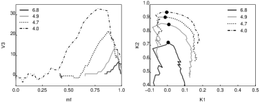
Figure 5.— The 4th Minkowski functional $V_{3}$ and the shapefinders $K_{1}$ (planarity) and $K_{2}$ (filamentarity) for the SGW for different density levels. The mass fraction in the left panel is that for the whole SGW at the density level $D=4.0$; for other density levels the superclusters start at higher mass fractions (sect. 3.3). In the right panel the mass fraction $m_{f}$ increases anti-clockwise along the curves. The filled circles in the right panel mark the value of the mass fraction $m_{f}=0.7$. In the $(K_{1},K_{2})$-plane filaments are located near the $K_{2}$-axis, pancakes near the $K_{1}$-axis, and ribbons along the diagonal. Solid black line corresponds to the density level $D=6.8$, solid grey line—$D=4.9$, dotted line—$D=4.7$, and dash-dotted line—$D=4.0$.

In the T10 catalogue the first ranked galaxy of a group is defined as the most luminous galaxy in the $r$-band. We will use the same definition in the present paper; later we will compare the properties of those first rank galaxies, which are BRGs, with those, which are not BRGs.

A 3D interactive PDF graph that shows the spatial distribution of groups of galaxies in the SGW can be found at {http://www.aai.ee/$∼$maret/SGWmorph.html}.

3. Morphology

3.1. Minkowski functionals and shapefinders

If we want to understand the formation, evolution and present-day properties of cosmic structures then we must use, in addition to the usual statistics that characterize the clustering of galaxies (the 2-point correlation function, Nth nearest neighbour and others, see Martínez & Saar, 2002, for a review about methods to characterize galaxy distribution) higher order statistics to describe structures like superclusters, filaments and clusters in which galaxies are embedded (Bond et al., 2010a). A number of methods are used to define and characterize cosmic structures (Pimbblet, 2005; Stoica et al., 2010; van de Weygaert et al., 2009; Aragón-Calvo et al., 2010; Bond et al., 2010a, b, and references therein). One possible approach is to determine cosmic structures (in our case—superclusters of galaxies) using, for example, a density field, and then to study their morphology (Schmalzing & Buchert, 1997; Sathyaprakash et al., 1998; Shandarin et al., 2004, and references therein).

Supercluster geometry (morphology) is defined by its outer (limiting) isodensity surface, and its enclosed volume. When increasing the density level over the threshold overdensity $D=4.7$ (Sect. 2.1), the isodensity surfaces move into the central parts of the supercluster. The morphology of the isodensity contours is (in the sense of global geometry) completely characterized by the four Minkowski functionals $V_{0}$–$V_{3}$ (we give the formulas in the Appendix B).

Minkowski functionals, genus, and shapefinders have been used earlier to study the morphology of the large scale structure in the 2dF and SDSS surveys (Hikage et al., 2003; Park et al., 2005; Saar et al., 2007; James et al., 2007; Gott et al., 2008) and to characterize the morphology of superclusters (Sahni et al., 1998; Basilakos et al., 2001; Kolokotronis et al., 2002; Sheth et al., 2003; Basilakos, 2003; Shandarin et al., 2004; Basilakos et al., 2006) in observations and simulations. These studies concern only the “outer” shapes of superclusters and do not treat their substructure. We expanded this approach in Einasto et al. (2007d), using the Minkowski functionals and shapefinders to analyze the full density distribution in superclusters, at all density levels.

The original luminosity density field, used to determine individual superclusters in the SGW and the full SGW complex, was calculated using all galaxies. To calculate the density field for the study of the morphology, we recalculated the density field for each individual structure under study. We used volume-limited galaxy samples and calculated the number density; this approach makes our results insensitive to selection corrections (although our SGW samples are almost volume-limited already, compare the numbers of galaxies in full and volume-limited samples, given in Table LABEL:tab:scldata and in the caption of Fig. 4). To obtain the density field for estimating the Minkowski functionals, we used a kernel estimator with a $B_{3}$ box spline as the smoothing kernel, with the radius of 16 $h^{-1}$ Mpc (Saar et al., 2007; Einasto et al., 2007d). As the argument labeling the isodensity surfaces, we chose the (excluded) mass fraction $m_{f}$—the ratio of the mass in regions with density lower than the density at the surface, to the total mass of the supercluster. When this ratio runs from 0 to 1, the iso-surfaces move from the outer limiting boundary into the center of the supercluster, i.e. the fraction $m_{f}=0$ corresponds to the whole supercluster, and $m_{f}=1$ to its highest density peak. This is the convention adopted in all papers devoted to the morphology of the large-scale galaxy distribution. The reason for this convention (the higher the density level, the higher the value of the mass fraction) is historical—the most popular argument for the genus and for the Minkowski functionals has been the volume fraction that grows with the density level; all other arguments are chosen to run in the same direction. We refer to Einasto et al. (2007d) for details of the calculations of the density field.

For a given surface the four Minkowski functionals (from the first to the fourth) are proportional to: the enclosed volume $V$, the area of the surface $S$, the integrated mean curvature $C$, and the integrated Gaussian curvature $\chi$. Last of them, the fourth Minkowski functional $V_{3}$ describes the topology of the surface; at high densities it gives the number of isolated clumps (balls) in the region, at low densities – the number of cavities (voids) (see, e.g. Saar et al., 2007).

The fourth Minkowski functional $V_{3}$ is well suited to describe the clumpiness of the galaxy distribution inside superclusters—the fine structure of superclusters. We calculate $V_{3}$ for galaxies of different populations in superclusters for a range of threshold densities, starting with the lowest density used to determine superclusters, up to the peak density in the supercluster core. So we can see in detail how the morphology of superclusters is traced by galaxies of different type.

In addition to the fourth Minkowski functional $V_{3}$ we use the dimensionless shapefinders $K_{1}$ (planarity) and $K_{2}$ (filamentarity) (Sahni et al., 1998) (Appendix B). In Einasto et al. (2007d) we showed that in the $(K_{1},K_{2})$ shapefinder plane the morphology of superclusters is described by a curve (morphological signature) that is similar for all multi- branching filaments. In the present paper we will use the morphological signature to characterize the morphology of superclusters and of galaxy populations in them.

There are two main effects that affect the reconstructed density field and its Minkowski functionals. The first is due to the fact that about 6-7% of galaxy redshifts are missing, because of fiber collisions (Zehavi, I. and the SDSS Collaboration et al., 2010). About 60% of these are approximately at the same distance as their close neighbours (Zehavi et al., 2002), but others are not. We found the collision groups in the SDSS, determined the galaxies that do not have redshifts because of fiber collisions, and ran Monte- Carlo simulations, assigning to 60% of randomly selected non-redshift galaxies the redshift of their neighbours. Other 40% of non-redshift galaxies were omitted, assuming that their true redshift will take them out of the supercluster. This procedure should give upper limits for errors. We ran 1000 simulations and found that both the morphological signatures and $V_{3}$ did not change (at the 95% confidence level) – fiber collisions are too scarce to affect the estimates of the morphological characteristics.

Another effect is the discreteness of galaxy catalogues (shot noise) that induces errors in the density estimates. To take this into account we have to define first the statistical model for the spatial distribution of galaxies within a supercluster. One possibility is to use the Cox model, where we have a realization of a random field and a Poisson point process populates the supercluster by dropping galaxies there with the intensity proportional to the value of the realization in the neighbourhood of a possible galaxy. We tested that model and found that it is not able to describe the structure of superclusters; we summarize the results in App. D.

After several erroneous approaches, we used the popular halo model ideology (see Cooray & Sheth, 2002; Yang et al., 2007; van den Bosch et al., 2007, and references therein for details) to define a statistical model for superclusters. We assume that supercluster structure is defined by its dark matter haloes, and discreteness errors are caused by the random positions of galaxies within these haloes. As the halo model assumes that the main galaxy of a halo lies at its centre, the main galaxies of our groups and the isolated galaxies (the main galaxies of haloes where other galaxies are too faint to see) remain fixed. For satellite galaxies, we use smoothed bootstrap to simulate the distribution of satellites inside our haloes – we select satellite galaxies by replacement, and add to their spatial positions increments with the same distribution as the $B_{3}$ kernel we use for density estimation. Smoothed bootstrap is known to be able to estimate pointwise errors of densities (Silverman & Young, 1987; Davison & Hinkley, 2009). As the the $B_{3}$ spline (Eq.A3) practically coincides with a Gaussian of the rms deviation $\sigma=0.6$, we define the $B_{3}$ kernel width $a=\sigma_{r}/0.6$ for every halo (galaxy group) using the rms deviation $\sigma_{r}$ of the radial positions of galaxies for that group. We generated mock superclusters with new galaxy distributions by smoothed bootstrap and calculated again the density field and Minkowski functionals, repeating this procedure 1000 times. The figures in Sect. 3.4, where we compare the Minkowski functionals and shapefinders for galaxy populations of different superclusters in the SGW show the 95% confidence regions obtained by these simulations.

3.2. Minkowski functionals and shapefinders—general

Next we describe shortly how the 4th Minkowski functional $V_{3}$ and the shapefinders $K_{1}$ and $K_{2}$ describe the morphology of a system.

At small mass fractions the isosurface includes the whole supercluster and the value of the 4th Minkowski functional $V_{3}=1$. As we move to higher mass fractions, the isosurface includes only the higher density parts of superclusters. Individual high density regions in a supercluster, which at low mass fractions are joined together into one system, begin to separate from each other, and the value of the 4th Minkowski functional ($V_{3}$) increases. At a certain density contrast (mass fraction) $V_{3}$ has a maximum, showing the largest number of isolated clumps in a given supercluster. The 4th Minkowski functional $V_{3}$ depends also on the number of tunnels, which may appear in the supercluster topology, as part of the galaxies do not contribute to the supercluster at intermediate density levels. At still higher mass fractions only the high density peaks remain in the supercluster and the value of $V_{3}$ decreases again.

When we increase the mass fraction, the changes in the morphological signature accompany the changes of the 4th Minkowski functional. As the mass fraction increases, at first the planarity $K_{1}$ almost does not change, while the filamentarity $K_{2}$ increases – at higher density levels superclusters become more filament-like than the whole supercluster. Then also the planarity starts to decrease, and at a mass fraction about $m_{f}=0.7$ the characteristic morphology of a supercluster changes – we see the crossover from the outskirts of a supercluster to the core of a supercluster (Einasto et al., 2007d).

3.3. Morphology of the SGW

We calculate the Minkowski functionals and shapefinders for superclusters in the SGW, defined at four different density levels, to see the change of the morphology of the SGW with density (Fig. 5). In the left panel of this figure the individual mass fractions for higher density levels are rescaled and shifted so that they show the fraction of mass of systems at a high density level relative to the total mass of the systems at the lowest density level, $D=4.0$.

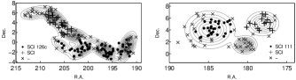
Figure 6.— The sky distribution of galaxies and BRGs in the superclusters SCl 126 and SCl 111. The distribution of galaxies in the whole supercluster (at the density level $D=4.9$) is shown by density contours. Dots mark groups with BRGs which belong to superclusters at the density level $D=6.8$, crosses mark groups with BRGs in other systems at this density level, which have not joined the superclusters SCl 126 and SCl 111 yet, and x-s mark groups with BRGs which at this density level do not belong to any system.

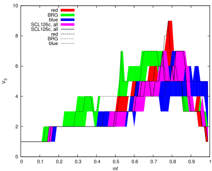
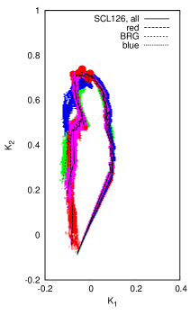
Figure 7.— The 4th Minkowski functional $V_{3}$ (left panel) and the shapefinders $K_{1}$ (planarity) and $K_{2}$ (filamentarity) (right panel) for the red and blue galaxies and the BRGs in the core of the supercluster SCl 126 (SCl 126c). The black line denotes $V_{3}$ for all galaxies (given for comparison, this is the same line as in Fig. 5 for the density level $D=6.8$, but here the mass fraction is not rescaled), dashed line with long dashes—red galaxies, dashed line with short dashes—BRG-s, and dotted line—blue galaxies. The filled circles in the right panel mark the value of the mass fraction $m_{f}\approx 0.7$. The colored regions in this and the next two figures show the 95% confidence regions obtained by bootstrap simulations as explained in text. With red color we show the confidence regions for red galaxies, blue corresponds to blue galaxies, green to BRGs and magenta to the full supercluster.

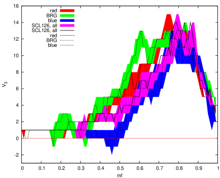
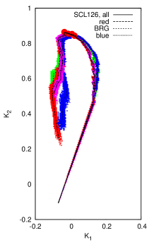
Figure 8.— The 4th Minkowski functional $V_{3}$ and the shapefinders $K_{1}$-$K_{2}$ for the red and blue galaxies and the BRGs in the whole supercluster SCl 126. The lines and colored regions correspond to galaxy populations as explained in Fig 7. Again, for comparison we show $V_{3}$ and $K_{1}$-$K_{2}$ lines for the full supercluster. The filled circles in the right panel mark the value of the mass fraction $m_{f}\approx 0.7$.

At the highest density level ($D=6.8$) only the core region of the supercluster SCl 126 contributes to the SGW. The left panel of Fig. 5 shows that for this core, the value of the 4th Minkowski functional $V_{3}$ is small almost over the whole range of mass fractions, the largest value of $V_{3}$ is 5. The right panel of Fig. 5 shows the corresponding morphological signature, with the starting planarity $K_{1}\approx 0.1$. As the mass fraction increases, the filamentarity $K_{2}$ increases and reaches a maximum value of about 0.72 at the mass fraction $m_{f}=0.7$, when the morphological signature changes. The shape of the morphological signature $K_{1}$- $K_{2}$ is consistent with a single filament (see for details Einasto et al., 2007d).

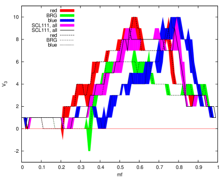
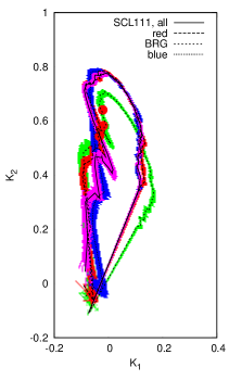
Figure 9.— The 4th Minkowski functional $V_{3}$ and the shapefinders $K_{1}$- $K_{2}$ for the red and blue galaxies and the BRGs in the supercluster SCl 111. The lines and colored regions correspond to galaxy populations as explained in Fig 7. The filled circles in the right panel mark the value of the mass fraction $m_{f}\approx 0.7$.

At the density level $D=4.9$ new galaxies join the SGW and the SGW coincides with the whole supercluster SCl 126. The maximum value of the clumpiness $V_{3}=12$, and the values of the planarity $K_{1}$ and filamentarity $K_{2}$ are larger – the morphology of the supercluster resembles a multibranching filament (Einasto et al., 2007d), as shown by the morphological signature.

At the density level $D=4.7$ the supercluster SCl 111 also joins the SGW (Fig. 1, right panel). The maximum value of the 4th Minkowski functional $V_{3}=20$. In the $(K_{1},K_{2})$-plane the morphological signature describes a planar system (Einasto et al., 2007d).

At a still lower density level, $D=4.0$, the superclusters which really do not belong to the SGW, join into one system with the SGW (Fig. 1, right panel). The maximum value of the 4th Minkowski functional $V_{3}=33$, and in the $(K_{1},K_{2})$-plane the morphological signature becomes even more typical of a planar system, consisting of more than one individual supercluster. Interestingly, although the overall morphology changes strongly, we see that in all cases, the morphological signature changes at a mass fraction $m_{f}\approx 0.7$, a change of morphology at a crossover from the outskirts to the core regions (Einasto et al., 2008).

At high mass fractions, in addition to the core of the supercluster SCl 126, also other high density clumps contribute to the full SGW, thus they also add their contribution to the values of the 4th Minkowski functional $V_{3}$ and to $K_{1}$ and $K_{2}$ in Fig. 5. Thus in Fig. 5 the values of $V_{3}$ for the density level, say, $D=4.9$, at mass fractions which correspond to the density level $D=6.8$ (approximately, in Fig. 5 this corresponds to the mass fraction $mf=0.85$) are larger than those from the density level $D=6.8$ at the same mass fraction. In other words, the curves characterizing the morphology of the SGW at different density levels depend on all the systems encompassed by the density iso-surfaces.

3.4. Morphology of galaxy populations in the superclusters SCl 126 and SCl 111

Next we calculate the 4th Minkowski functional $V_{3}$ and the morphological signature $K_{1}$-$K_{2}$ for individual galaxy populations defined by their $g-r$ color, and for the BRGs, in the two richest superclusters in the SGW: the superclusters SCl 126 (separately for the core and for the whole supercluster) and SCl 111 (Fig. 7 – Fig. 9). We show in figures the 95% confidence regions obtained by Monte-Carlo simulations as explained in sect. 3.1.

To help to understand the results of these calculations we show in Fig. 6 the sky distribution of galaxies in the superclusters SCl 126 and SCl 111. The distribution of all galaxies in the full superclusters is delineated with 2D density contours. The location of groups with BRGs (we discuss the group membership of BRGs in the next section) is shown with different symbols—dots mark the members of both superclusters SCl 126 and SCl 111 at a high density level, $D=6.8$, crosses mark members of another systems at this density level (these systems have not yet joined the superclusters SCl 126 and SCl 111, correspondingly), and x-s mark groups with BRGs which do not belong to any supercluster at the density level $D=6.8$ yet, but will be the members of the superclusters SCl 126 and SCl 111 at the density level $D=4.9$.

In Fig. 7 we present the results of the calculations of the Minkowsky functional $V_{3}$ and the shapefinders for the core of the supercluster SCl 126c (the groups with BRGs in this system are marked with dots in Fig. 6). Fig. 7 shows that the clumpiness of red and blue galaxies and BRGs is rather similar over the whole range of mass fractions $m_{f}$. The BRGs form some clumps at the mass fractions $m_{f}=$0.3–0.4 and $m_{f}=$0.5–0.7, which are not seen in the distribution of red and blue galaxies; their spatial distribution is less clumpy at these densities. The confidence regions show that these differences are statistically significant at least at the 95% confidence level.

At the mass fraction $m_{f}=0.8$ the clumpiness of red galaxies is the largest, reaching the value $V_{3}=9$. The differences between the clumpiness of red galaxies and other galaxy populations are statistically significant at least at the 95% confidence level. The clumpiness of blue galaxies and BRGs reaches the same value at the mass fraction $m_{f}=0.80$. At a higher mass fraction, $m_{f}=0.9$, blue galaxies form some isolated clumps and the value of $V_{3}$ for blue galaxies is larger than that for red galaxies and BRGs ($V_{3}=5$ and $V_{3}\leq 3$, correspondingly). At these highest mass fractions the differences between the clumpiness of blue and all other galaxy populations are statistically significant at least at the 95%confidence level.

The morphological signatures of galaxies from different populations almost coincide at the mass fractions $m_{f}<0.7$ (in the outskirts of the supercluster). The morphological signature for the core of the supercluster SCl 126c is characteristic of a filament (Einasto et al., 2007d). In this filament the distribution of galaxies from different populations is rather homogeneous, showing similar clumpiness and morphological signatures.

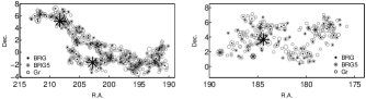
Figure 10.— The distribution of groups (Gr) and BRGs in the superclusters SCl 126 (left panel), and SCl 111 (right panel), in the sky. Empty circles show the location of groups, with symbol sizes proportional to the richness of the group. Dots mark groups which host up to four BRGs (denoted as BRG), stars—groups with five or more BRGs (BRG5). The three largest stars denote groups with the largest number of BRGs in each system (the core of the supercluster SCL 126, SCl 126c, the outskirts of this supercluster, SCl 126o, and the supercluster SCl 111).

In Fig. 8 we show the 4th Minkowski functional $V_{3}$ and the morphological signature $K_{1}$-$K_{2}$ for the whole supercluster SCl 126. This figure reveals several differences in comparison with the core of the supercluster. At the mass fractions $0.15<m_{f}<0.25$ BRGs form some isolated clumps (for BRGs, $V_{3}=3$) while $V_{3}$ for red galaxies has a small minimum ($V_{3}=0$) suggesting that at a low density level in the outskirts of the supercluster there are differences in how the substructure of the supercluster is delineated by BRGs and red galaxies. The value of the 4th Minkowski functional $V_{3}$ for red galaxies ($V_{3}=0$) suggests that the population of red galaxies may have tunnels through them at these mass fractions (see Appendix B). But the differences between the clumpiness of red galaxies and BRGs at this mass fraction interval are not statistically significant at the 95% confidence level, as show the confidence regions in Fig. 8.

At the mass fractions $m_{f}\approx 0.3$ the clumpiness of red galaxies and BRGs increases, while the clumpiness of blue galaxies decreases and even becomes negative. This means that at intermediate densities (up to $m_{f}\approx 0.6$), red galaxies and BRGs form isolated clumps, while blue galaxies are located in lower density systems which at these mass fractions do not contribute to the supercluster. Some of these isolated clumps belong to a separate system, marked with crosses in Fig. 6 (left panel). Negative values of $V_{3}$ for blue galaxies at mass fractions $m_{f}\approx 0.45$ suggest that these systems have tunnels through them. These systems belong to the outskirts of the supercluster SCl 126. At this mass fraction interval the differences between the clumpiness of red galaxies and BRGs, and of blue galaxies, are statistically significant at least at the 95% confidence level.

At higher mass fractions, $m_{f}\geq 0.5$, the clumpiness of blue galaxies increases. The clumpiness of red and blue galaxies reaches a maximum value, $V_{3}=13$, at mass fractions $m_{f}=$0.7–0.8, where the morphological signature shows a change of the morphology of the supercluster. At still higher mass fractions we do not see differences between the fourth Minkowski functionals of galaxy populations which are statistically significant at the 95% confidence level.

For the most of the mass fraction interval, the clumpiness of red galaxies is larger than the clumpiness of blue galaxies. The differences between the morphological signatures of red and blue galaxies are statistically significant for the high mass fractions at the 95% confidence level.

Fig. 9 shows the 4th Minkowski functional $V_{3}$ and the morphological signature $K_{1}$-$K_{2}$ for another rich supercluster in the SGW, the supercluster SCl 111. The curves of $V_{3}$ differ from those for the supercluster SCl 126. At mass fractions $0.15<m_{f}<0.35$ the $V_{3}$ curves suggest that red galaxy and BRG populations have tunnels through them. At these mass fractions some galaxies already do not contribute to the supercluster (these are galaxies which do not belong to any supercluster at higher density levels in Fig. 6) so that tunnels can form. In the same time individual clumps are connected, so that tunnels form between them (otherwise red galaxies and BRGs would form isolated clumps instead of tunnels). At mass fractions $m_{f}>0.35$ the value of $V_{3}$ for red galaxies and BRGs increases showing that the number of isolated clumps formed by these galaxies grows. The $V_{3}$ curves for red galaxies and BRGs reach a maximum value ($V_{3}=$9–10) at a mass fraction $m_{f}\approx 0.6$ and then decrease. Such a clumpiness curve is characteristic of a poor supercluster, a system dominated by a few high density clumps with rich clusters in it (a spider, see Einasto et al., 2007d). Fig. 6 (right panel) shows low density regions (groups which do not belong to any supercluster at densities $D=6.8$) and high density regions which form systems already at densities $D=6.8$ in this supercluster.

The value of the 4th Minkowski functional $V_{3}$ for blue galaxies in the supercluster SCl 111 $V_{3}=1$ up to mass fractions $m_{f}<0.3$ shows that at these mass fractions blue galaxies form one system without isolated clumps or tunnels through them. In other words, in the outskirts of this supercluster blue galaxies are distributed more homogeneously than red galaxies or BRGs. In the mass fraction interval $0.35<m_{f}<0.45$ the value of $V_{3}$ for blue galaxies decreases—some blue galaxies do not contribute to supercluster any more and tunnels form. At the mass fraction $m_{f}>0.45$ the value of $V_{3}$ increases (the number of isolated clumps increases) and reaches the maximum ($V_{3}=9$) at the mass fraction $m_{f}=0.8$. After that, the clumpiness of blue galaxies decreases.

In Fig. 9 we see that at almost the whole mass fraction interval the differences between the values of the 4th Minkowski functional $V_{3}$ for galaxies from different populations are statistically significant at least at the 95% confidence level.

The morphological signature of the supercluster SCl 111 also differs from that of the supercluster SCl 126. The values of the planarity $K_{1}$ at small mass fractions are larger than those for the SCl 126, and the maximum values of the filamentarity $K_{2}$ are lower ($K_{2}\leq 0.7$, while for the supercluster SCl 126 the filamentarity $K_{2}\leq 0.9$). Interestingly, for certain mass fractions ($0.45<m_{f}<0.65$) the planarity of BRGs is larger than that of red and blue galaxies. This may be due to the large clumpiness of BRGs in the same mass fraction interval (Fig. 9, left panel).

Fig. 9 shows that the differences between morphological signatures of red galaxies, BRGs and blue galaxies are statistically significant at the 95% confidence level at a wide range of mass fractions.

3.5. Summary

We have seen that the morphology of the SGW varies from a simple filament to a multibranching filament and then, as we lower the level of the density, becomes characteristic of a very clumpy, planar system. The changes in morphology suggest, in addition to the analysis of the properties of individual superclusters (their richnesses and sizes), that a proper density level to delineate individual superclusters is $D=4.9$. A lower density level, $D=4.7$, can be used to select the whole SGW.

The overall morphology of the galaxy systems in the SGW region changes strongly when we change the density level, but in all cases, the morphological signature changes at a mass fraction $m_{f}\approx 0.7$, at a crossover from the outskirts to the core regions of superclusters.

The morphology of the core of the supercluster SCl 126 is characteristic of a simple filament with small clumpiness. Differences between the clumpiness and morphological signatures of individual galaxy populations are small, telling us that all galaxy populations delineate the core of the supercluster in the same way. The morphology of the whole supercluster SCl 126 can be described as characteristic of a multibranching filament, where the clumpiness of red galaxies and BRGs is larger than the clumpiness of blue galaxies, especially in the outskirts of the supercluster. The supercluster SCl 111 resembles a multispider (we described the morphological templates in more detail in Einasto et al., 2007d). Here again the clumpiness of red galaxies and BRGs is larger than the clumpiness of blue galaxies. In the outskirts of both superclusters blue galaxies are distributed more homogeneously than red galaxies and BRGs. In the outskirts of superclusters galaxy populations have tunnels through them.

The morphology of superclusters can be characterized by the ratio of the shapefinders, $K_{1}/K_{2}$ (the shape parameter). This approach was used, for example, by Basilakos (2003) to study the shapes of superclusters— a large value of this ratio indicates planar systems. Our calculations show that the values of the shape parameter are as follows: for the core of the supercluster SCl 126, SCl 126c, $K_{1}/K_{2}\approx 0.33$ and for the full supercluster SCl 126 $K_{1}/K_{2}\approx 0.28$; we get the same value for all galaxy populations. In the supercluster SCl 111, $K_{1}/K_{2}=0.47$ for the full supercluster and for red galaxies, while for BRGs $K_{1}/K_{2}=0.52$ and for blue galaxies $K_{1}/K_{2}=0.61$. This is another difference between the superclusters in the SGW.

We assessed the statistical significance of the differences between the 4th Minkowski functional $V_{3}$ and morphological signatures of different galaxy populations in superclusters using Monte-Carlo simulations and showed that at least at some mass fraction intervals (depending on the populations) the differences between the galaxy populations are statistically significant at least at the 95% confidence level.

4. BRGs and the first ranked galaxies in the superclusters SCl 126 and SCl 111

Table 2The properties of groups with and without BRGs in the SCl 126 and SCl 111.

(1)	(2)				(3)
Region	Gr, BRG				Gr, –
SCl ID	$N_{\mbox{gr}}$	$N_{\mbox{gal, m}}$	$\sigma_{\mbox{m}}$	$L_{\mbox{tot, m}}$	$N_{\mbox{gr}}$	$N_{\mbox{gal, m}}$	$\sigma_{\mbox{m}}$	$L_{\mbox{tot, m}}$
SCl 126c	67	12.1	250.5	20.2	98	2.9	135.8	3.5
SCl 126o	101	9.1	209.0	13.7	112	2.9	125.9	3.6
SCl 111	85	9.6	199.2	13.1	116	2.6	138.2	2.7

Figure 11.— The number of BRGs in groups, $N_{BRG}$, in the superclusters SCl 126 (separately for the core, SCl 126c and for the outskirts, SCl 126o) and SCl 111 vs the richness of groups (the number of galaxies in groups, $N_{gal}$), where the BRGs are located. Filled circles—SCl 126c, empty circles—SCl 126o, crosses—SCl 111.

As the Minkowski functionals found in the previous section demonstrated, the morphology of the superclusters SCl 126 and SCl 111 is different. The supercluster SCl 126, especially its high density core region, is a multibranching filament of a high overall density. The supercluster SCl 111 consists of three loosely located, less dense concentrations (see also Fig. 6). The Minkowski functionals show several similarities and differences between the way how the substructure of superclusters is delineated by different galaxy populations.

In this section we focus on the comparison of galaxy and group content in different superclusters of the SGW to search for other possible differences between them, in addition to the differences in morphology. We study the properties of BRGs and those first ranked galaxies, which are not BRGs. In the case of the supercluster SCl 126 we consider separately the core region, SCl 126c, and the outskirts, SCl 126o. We analyze the group membership of BRGs, as well as the colors, luminosities and morphological types of BRGs in the superclusters SCl 126 and SCl 111, calculate the peculiar velocities of BRGs and other first ranked galaxies in groups, and study the location of groups with different first ranked galaxies in superclusters.

4.1. Group membership of BRGs

Fig. 10 shows the sky distribution of the BRGs and galaxy groups in the superclusters SCl 126 (left panel) and SCl 111 (right panel). Here we plotted groups with symbols of size proportional to their richness. In this figure we mark those groups which host up to four BRGs with small dots and groups with at least five BRGs—with stars. The comparison with Fig. 6 shows that in the supercluster SCl 126 groups with a large number of BRGs are located both in the core and in the outskirts. In the supercluster SCl 111 assemblies of groups with a large number of BRGs form systems already at the density level $D=6.8$, while the poor groups and groups with a few BRGs in them do not belong to any supercluster at this density level.

Table 3BRGs and the first ranked galaxies in the SCl 126 and SCl 111.

(1)	(2)			(3)			(4)
Population ID	SCl 126c			SCl 126o			SCl 111
$N_{\mbox{gal}}$		1397			1765			1515
$f_{\mbox{r}}$		0.72			0.61			0.63
$ID$	B1	Bs	1nB	B1	Bs	1nB	B1	Bs	1nB
$N_{\mbox{gal}}$	67	114	98	101	140	159	85	123	135
$f_{\mbox{r}}$	0.93	0.96	0.64	0.93	0.87	0.49	0.93	0.93	0.47
$f_{\mbox{s}}$	0.39	0.42	0.59	0.35	0.58	0.82	0.45	0.51	0.77
$f_{\mbox{rs}}$	0.34	0.39	0.44	0.31	0.52	0.71	0.41	0.48	0.57
$N_{\mbox{merg}}$	9	14	1	3	10	4	13	12	6
$N_{\mbox{clock}}$	6	4	9	8	5	21	7	3	16
$N_{\mbox{a-clock}}$	4	15	14	9	6	21	4	13	16
$W_{\mbox{E}}$	0.031	0.030	0.036	0.029	0.027	0.066	0.031	0.034	0.073
$W_{\mbox{S}}$	0.060	0.052	0.035	0.047	0.060	0.039	0.042	0.058	0.058
$vE_{\mbox{pec}}$	186	467	132	141	260	133	154	269	178
$vS_{\mbox{pec}}$	154	285	109	205	290	101	164	397	105

The richest group in the core of the supercluster SCl 126, that corresponds to the Abell cluster A1750, located at $R.A\approx 202.7^{\circ}$ and $Dec\approx-1.9^{\circ}$ (Fig. 10, left panel) hosts a full 17 BRGs. In the outskirts of the supercluster SCl 126 the number of BRGs is the largest in a group that corresponds to the Abell cluster A1809, located at $R.A\approx 208.3^{\circ}$ and $Dec\approx 5.1^{\circ}$, this group hosts 12 BRGs; isolated clumps seen in the $V_{3}$ curve at mass fractions of about $m_{f}\approx 0.2$ (Fig. 8) are probably at least partly due to this group. In the supercluster SCl 111, the richest group corresponds to the Abell cluster A1516, located at $R.A\approx 184.4^{\circ}$ and $Dec\approx 3.7^{\circ}$, and hosts 15 BRGs. The location of the groups with the largest numbers of BRGs in Fig. 10 is marked with the largest stars.

In Fig. 11 we compare the number of BRGs in groups in the superclusters SCl 126 (in the core and in the outskirts) and in the supercluster SCL 111. This figure shows that most groups with BRGs host only a few BRGs (the mean number of BRGs in groups is 2 in both the superclusters SCl 126 and SCl 111). Groups with five or more BRGs are themselves also richer than groups with a smaller number of BRGs, with at least 20 member galaxies. Although the richest group in the core of the supercluster SCl 126c hosts more BRGs than the richest group in the outskirts of this supercluster, the overall membership of BRGs in groups is statistically similar in both these regions, and also in the supercluster SCl 111. Table LABEL:tab:GRBRG shows that approximately 40% of BRGs are first ranked galaxies in groups.

There are also BRGs, which do not belong to any group (isolated BRGs). In the core of the supercluster SCl 126, SCl 126c, 11% of all BRGs do not belong to groups, while in the outskirts of this supercluster this fraction is 18%. In the supercluster SCl 111 20% of all BRGs do not belong to groups. In this respect there is a clear difference between superclusters.

Tempel et al. (2009) showed, analysing the luminosity functions of galaxies in the 2dFGRS groups, that most of the bright isolated galaxies should be the first ranked galaxies of groups, where the fainter members are not observed since they fall outside of the observational window of the flux-limited sample. Thus we may suppose that there are no truly isolated BRGs, but they are the first ranked galaxies of fainter groups.

Fig. 10 shows that there are also many groups without BRGs (empty circles without a dot or a star). In the supercluster SCl 111 many of these groups are located loosely between the three concentrations of this supercluster (Fig. 10, right panel). We present the summary of the properties of groups with and without BRGs in superclusters in Table LABEL:tab:GRBRG. This table shows, firstly, that groups with BRGs are richer, have larger velocity dispersions and higher luminosities than groups without BRGs. Secondly, groups with BRGs in the core of the supercluster SCL 126, SCl 126c, are richer and have larger velocity dispersions and higher luminosities than groups with BRGs in the outskirts of this supercluster or groups in the supercluster SCl 111. The Kolmogorov-Smirnov test shows that the probability that the distributions of the properties of groups with BRGs in SCl 126c and SCl 126o are drawn from the same distribution is 0.04, and 0.01 for groups in SCl 126c and SCl 111. This shows another difference between these systems.

4.2. Colors, luminosities and morphological types of BRGs and the first ranked galaxies

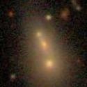
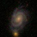
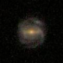
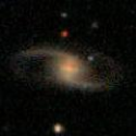
Figure 12.— SDSS images of some of the first ranked BRGs. From left to right: two galaxies from the core of the supercluster SCl 126 (with ID J131236.98-011151 and J133111.02-014338.2), a galaxy from the outskirts of the supercluster SCl 126 (J135143.99+045833.6), and a galaxy from the supercluster SCl 111 (J120652.46+035952.8).

Figure 13.— The color-magnitude relations for elliptical (empty circles) and spiral (filled circles), first ranked (upper row) and satellite (lower row) BRGs. Left panels: the core of the supercluster SCl126, middle panels: the outskirts of the supercluster SCl126, right panels: the supercluster SCl111.

Next we divide BRGs into two populations: the first ranked galaxies in groups and those which are not (we denote them as satellite BRGs). We compare the colors, luminosities and morphological types of these two sets of BRGs and those first ranked galaxies which are not BRGs in the two richest superclusters in the SGW, SCl 126 and SCl 111.

We summarize the colors and morphology of the galaxies of the two superclusters in Table LABEL:tab:sclgal. It shows that most BRGs are red, although a small fraction of BRGs have blue colors. The fraction of red galaxies among these first ranked galaxies, which are not BRGs, is smaller. We note that in the core of the supercluster SCl 126 the fraction of red galaxies among those first ranked galaxies which are not BRGs is larger and the fraction of spirals (and red spirals) among them is smaller than in the outskirts of this supercluster or in the supercluster SCl 111.

A large fraction of red galaxies in our sample are spirals. The images of some BRGs in the SGW are shown in Fig. 12. Galaxies with visible spiral arms are located in groups of different richness, and more than a half of them do not belong to any group. We see also that a considerable number of BRGs and the first ranked galaxies may be merging or have traces of past merging events.

The scatter plots of the colors of ellipticals and spirals among the first ranked and satellite BRGs are shown in Fig. 13 (see also Table LABEL:tab:sclgal). Both show that for the red elliptical first ranked galaxies the color scatter is small (about 0.03), while for the red spirals it is larger (0.04–0.06). Some satellite BRGs have blue colors. Fig. 13 shows that most BRGs with blue colors are spirals, but there are also two elliptical galaxies among them.

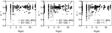
Figure 14.— The $g-r$ color vs the group richness of BRGs (filled circles) and the first ranked galaxies which are not BRGs (empty circles). Left panel: the core of the supercluster SCl126, middle panel: the outskirts of the supercluster SCl126, right panel: the supercluster SCl111.

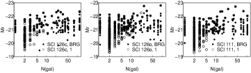
Figure 15.— The luminosity vs the group richness of BRGs (filled circles) and the first ranked galaxies which are not BRGs (empty circles). Left panel: the core of the supercluster SCl126, middle panel: the outskirts of the supercluster SCl126, right panel: the supercluster SCl111.

Fig. 14 and Fig. 15 show the colors and luminosities of BRGs and those first ranked galaxies, which are not BRGs, vs the number of galaxies in the groups where they reside. We see that the first ranked galaxies with bluer colors and also fainter first ranked galaxies and fainter BRGs reside in poor groups. In almost all groups with $N_{gal}>10$ the first ranked galaxy is a BRG. The Kolmogorov-Smirnov test shows that the probabilities that the colors and luminosities of BRGs and the first ranked galaxies in systems under study are drawn from the same distributions are very small.

Comparison of the richnesses of groups where elliptical or spiral BRGs reside shows that almost all the spiral first ranked BGRs belong to poor groups with less than 13 member galaxies. At the same time spiral, satellite BRGs can be found in groups of any richness.

Our results are consistent with those by Berlind et al. (2006) who showed that the first ranked galaxies in more luminous groups are more luminous than the first ranked galaxies in less luminous groups (see also Yang et al., 2008; Tempel et al., 2009, and references therein).

4.3. Peculiar velocities of BRGs and the first ranked galaxies

Next we calculated the peculiar velocities for the red ($g-r>0.7$) elliptical and spiral BRGs in three systems under study, for three sets of galaxies (the first ranked BRGs, satellite BRGs, and those first ranked galaxies, which are not BRGs) (Table LABEL:tab:sclgal).

Our calculations show that in both the superclusters SCl 126 and SCl 111 about half of the first ranked galaxies have large peculiar velocities. The largest peculiar velocities of the first ranked galaxies are even of the order of 1000 km/s.

In the supercluster SCl 126c, the peculiar velocities of elliptical BRGs are larger than those of spiral galaxies (both in the case of the first ranked galaxies and satellite BRGs). The statistical significance of differences of peculiar velocities between the elliptical and spiral first ranked galaxies is low, according to the Kolmogorov-Smirnov test. The differences between the peculiar velocities of elliptical and spiral satellite galaxies are statistically significant at the 95% confidence level.

In the superclusters SCl 126o and SCl 111 elliptical BRGs have smaller peculiar velocities than spiral BRGs, but those elliptical first ranked galaxies which do not belong to BRGs have larger peculiar velocities than spiral galaxies. The peculiar velocities of BRGs in these two superclusters are smaller than in the supercluster SCl 126c. According to the Kolmogorov- Smirnov test, these differences are statistically significant at the 92% level in both superclusters.

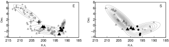
Figure 16.— The sky distribution of groups with at least 3 member galaxies with BRGs as their first ranked galaxy, in the supercluster SCl 126. Left panel—groups with elliptical first rank BRGs, right panel—groups with spiral first ranked BRGs. Different symbols correspond to different components determined with ’Mclust’, large symbols (in the case of triangles and circles - large filled symbols) correspond to these groups for which the uncertainty of the classification is larger than 0.05. Filled circles show the locations of groups, contours show the projected density levels calculated with ’Mclust’ (see text).

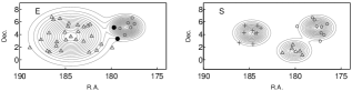
Figure 17.— The sky distribution of groups with at least 3 member galaxies with BRGs as their first ranked galaxy, in the supercluster SCl 111. Left panel—groups with elliptical first rank BRGs, right panel—groups with spiral first ranked BRGs. Symbols are as in Fig. 16. Contours show the projected density levels.

4.4. Sky distribution of groups with elliptical and spiral BRGs as the first ranked galaxy

Now we compare the distribution of groups with elliptical and spiral BRGs as their first ranked galaxies in the sky (Fig. 16 and Fig. 17). These figures show that in both superclusters the groups with elliptical first ranked BRGs fill the supercluster volume in a much more uniform manner than the groups with the spiral first ranked BRG. This was unexpected, since groups with an elliptical BRG as the first ranked galaxy are richer, and, as we showed, groups in the core of the supercluster SCl 126 are richer than in other systems under study.

To quantify the distribution of groups in superclusters (substructure of superclusters) and to calculate the projected density contours, we have used the R package ’Mclust’ (Fraley & Raftery, 2006). This package builds normal mixture models for the data, using multidimensional Gaussian densities with varying shape, orientation and volume. It finds the optimal number of concentrations, the corresponding classification (membership of each concentration), and the uncertainty of the classification. The uncertainty of the classification is defined using the probabilities for each galaxy to belong to a particular component and is calculated as 1. minus the highest probability of a galaxy to belong to a component. The uncertainty of the classification can be used as a statistical estimate how well groups are assigned to the components.

To measure how well components are determined and to find the best model for a given dataset, ’Mclust’ uses the Bayes Information Criterion (BIC) that is based on the maximized loglikelihood for the model, the number of variables and the number of mixture components. The model with the smallest value of BIC among all models calculated by ’Mclust’ is considered the best. For details we refer to Fraley & Raftery (2006).

We present the results in Fig. 16 and Fig. 17. In these figures we plot components of the best model according to BIC, determined by ’Mclust’ in the distribution of groups with elliptical and spiral BRGs as the first ranked galaxies with different symbols, large symbols (in the case of triangles and circles - large filled symbols) correspond to these groups for which the uncertainty of the classification is larger than 0.05. Groups with spiral BRGs as the first ranked galaxies in the supercluster SCl 111 all have the uncertainty of the classification smaller than 0.05.

Fig. 16 and Fig. 17 show that groups with elliptical and spiral BRGs as the first ranked galaxies populate superclusters in a different manner. In the supercluster SCl 126 groups with elliptical BRGs as the first ranked galaxies form three concentrations in the supercluster, and groups with a spiral BRG as the first ranked galaxy form two concentrations. The mean uncertainty of the classification calculated by ’Mclust’ for the groups with elliptical first ranked BRGs is $2.0\cdot 10^{-3}$, for the groups with spiral first ranked BRGs it is $2.0\cdot 10^{-4}$. Very small uncertainties show very high probabilities for groups to belong to a particular component. Groups with the largest uncertainties of the classification are located there where components are overlapping.

For every dataset we analyzed in detail three best models found by ’Mclust’. For groups with elliptical BRGs as the first ranked galaxies in the supercluster SCl 126 two best models have three, the third even four components. The best model with two components for these groups is, according to BIC, very unlikely, and in this case ’Mclust’ collects together into one component groups indicated with circles and triangles in Fig. 16. These components differ from those determined using groups with spiral BRGs as the first ranked galaxies in this supercluster Fig. 16.

In the supercluster SCl 111 the groups with an elliptical BRG as the first ranked galaxy form two barely separated concentrations in the supercluster, and with spiral first ranked BRGs—three well-defined concentrations (Fig. 17). The mean uncertainty of the ’Mclust’ classification for the groups with elliptical first ranked BRGs is $9.4\cdot 10^{-9}$, for the groups with spiral first ranked BRGs $7.5\cdot 10^{-7}$.

The best model with three components for groups with elliptical BRGs as the first ranked galaxies in the supercluster SCl 111 is, according to BIC, much less likely. In this model groups from the component shown by triangles in Fig. 17 are divided between two components, the leftmost groups forming a separate component. Thus components differ from those determined in the distribution of groups with spiral BRGs as the first ranked galaxies in this supercluster.

If the components have a regular shape (ellipsoids or circles) as in the supercluster SCl 111 (Fig. 17, the component with mean coordinates $R.A\approx 184.4^{\circ}$ and $Dec\approx 3.67^{\circ}$) the scatter of the sky coordinates can be used to estimate the compactness/looseness of the sky distribution of groups in components. The rms scatter of coordinates in the case of groups with elliptical first ranked BRGs is $\sigma\approx 3.9^{\circ}$, for groups with spiral first ranked BRGs—$\sigma\approx 0.8^{\circ}$ that shows a more compact distribution of groups with spiral first ranked galaxies in this component. However, in the supercluster SCl 126 the sky distribution of groups is such that the scatter of coordinates of all components is large (Fig. 16) so we cannot use this estimate. In this supercluster we compared the fraction of groups with spiral and elliptical first ranked BRGs in the core and the outskirts of the supercluster. A full 47% of groups with a spiral first ranked BRG lie in the core region, while among groups with an elliptical BRG as the first ranked galaxy only 39% lie in the core region.

The number of groups with an elliptical first ranked galaxy in both superclusters is larger than the number of groups with a spiral first ranked galaxy. Thus we can resample groups with an elliptical first ranked galaxy by diluting randomly the sample of groups so that in the final sample the number of groups is equal to the number of groups with a spiral first ranked galaxy, and then run ’Mclust’ again to search for components among the resampled set of groups. However, a word of caution is needed – if ’Mclust’ will detect a different number of components among the randomly resampled groups compared to the original sample, the sky coordinates of these components depend on this particular realization of the resampling. We run the resampling procedure for both superclusters 10000 times. Our calculations showed that in the supercluster SCl 126, in about 27% of all cases ’Mclust’ detected in the distribution of groups with an elliptical first ranked galaxy two components, as in the case of the groups with a spiral first ranked galaxy, but the sky coordinates of these components varied strongly, covering the whole right acsension and declination interval of the supercluster SCl 126. The same is the case with the supercluster SCl 111, where ’Mclust’ detected in 14% of cases three components in resampled groups with an elliptical first ranked galaxy. This shows that when groups with an elliptical first ranked galaxy are resampled to the same number of objects as groups with spiral first ranked galaxy there is no clear difference in number of components between samples.

To understand better the differences between the distribution of groups with elliptical and spiral first ranked galaxies in superclusters a study of a larger sample of superclusters is needed.

We note that Berlind et al. (2006) showed that the groups with first ranked galaxies with bluer colors are more strongly clustered than the groups with the first ranked galaxies with redder colors. In contrast, Wang et al. (2008) showed that SDSS groups with red central galaxies are more strongly clustered than groups of the same mass but with blue central galaxies. As we showed, colors and morphological types of galaxies are not well correlated. Therefore, we plan to study a larger sample of groups with the with the first ranked galaxies of different morphological type and color in a larger set of superclusters to search for possible differences in their distribution.

4.5. Summary

The comparison of the group membership and properties (colors, luminosities and morphological types), as well as the peculiar velocities and the sky distribution of BRGs and those first ranked galaxies which are not BRGs in the two SGW superclusters revealed a number of differences between these superclusters.

In all three systems under study (the core and the outskirts of the supercluster SCl 126, and the supercluster SCl 111) rich groups with at least 20 member galaxies host at least five BRGs, the richest group in the supercluster SCl 126 in the core of the supercluster hosts even 17 BRGs. The fraction of those BRGs which do not belong to any group in the core of the supercluster SCl 126 (SCl 126c), is about two times smaller than in other systems under study.

In the core of the supercluster SCl 126 (SCl 126c), groups with BRGs are richer and have larger velocity dispersions than groups with BRGs in the outskirts of this supercluster and in the supercluster SCl 111.

In the core of the supercluster SCl 126 (SCl 126c) the fraction of red galaxies among those first ranked galaxies, which are not BRGs, is larger and the fraction of spirals among them is smaller than in the outskirts of this supercluster and in the supercluster SCl 111.

About 1/3 to 1/2 of all BRGs are spirals. The scatter of the $g-r$ colors of elliptical BRGs is about two times smaller than of spiral BRGs, showing that elliptical BRGs form a much more homogeneous population than spiral BRGs.

Peculiar velocities of elliptical BRGs in the core of the supercluster SCl 126 (SCl 126c) are larger than those of spiral BRGs, while in the outskirts of this supercluster, as well as in the supercluster SCl 111, the situation is opposite. Since both elliptical and spiral satellite BRGs lie in groups of all richnesses, this difference is not caused by the richness of the host group (this could be the case if spiral satellites were residing preferentially in poor groups). In the core of the supercluster SCl 126 (SCl 126c) the peculiar velocities of galaxies are larger than in the superclusters SCl 126o and SCl 111 suggesting that groups in the core of the supercluster SCl 126 are dynamically more active than those in other two systems under study.

In the two superclusters, groups with an elliptical first ranked BRG are located more uniformly than groups with a spiral first ranked BRG.

We note that, as we saw in section 3.3, although the outskirts of the supercluster SCl 126o and the supercluster SCl 111 are determined by a lower density level than the core of the supercluster SCl 126c, they contain high density regions. Thus the differences between the systems are not entirely due to the differences in density.

5. Discussion

5.1. Morphology of the superclusters

We analyzed recently the morphology of individual superclusters, applying Minkowski functionals and shapefinders, and using the full density distribution in superclusters, at all density levels (Einasto et al., 2007d, 2008). In these papers we used data from the 2dFGRS to delineate the richest superclusters and to study their morphology, as well as the morphology of individual galaxy populations.

Our studies included also the supercluster SCl 126, the richest supercluster in the SGW. Comparison of the results shows several differences and similarities. Due to sample limits a part of the supercluster SCl 126 was not covered by the 2dFGRS. This is seen in Fig. 10 (left panel) that shows an extended filament at the declinations $\delta>2^{\circ}$ not visible in the 2dFGRS data. Due to this, the clumpiness of galaxies in this supercluster ($V_{3}\leq 10$) in Einasto et al. (2008) was smaller than that found here; there are also small differences between the morphological signatures of this supercluster found here and in Einasto et al. (2008). Both studies showed that the differences between the clumpiness of red and blue galaxies are larger in the outskirts of the supercluster and smaller in the core of the supercluster. This shows that the scale-dependent bias between the 2dFGRS and SDSS due to the $r$-band selection of the SDSS (Cole et al., 2007) does not affect (strongly) the values of the Minkowski functionals.

However, even in the present study, using the data from the SDSS DR7, we cannot be sure that the SGW is fully covered by the observations. At low declinations, the SGW extends down to the DR7 limit, and it may be possible that the SGW continues at lower declinations. Future observations are needed to see the total extent of the SGW.

Our present study showed that the peculiar morphology of the supercluster SCl 126 is especially strongly expressed in the core region of the supercluster. The morphology of another supercluster in the SGW, the supercluster SCl 111, resembles that of simulated superclusters studied in Einasto et al. (2007d). This agrees with our comparison of the morphology of individual richest superclusters (Einasto et al., 2007d) in observations and in simulations that showed that the morphology of the simulated superclusters differs from the morphology of the supercluster supercluster SCl126.

The morphology of the full supercluster SCl 126 can be described as a multibranching filament while the core of this supercluster resembles a very rich filament with only a small number of clumps at high density levels. This makes the core of the supercluster SCl 126 an extreme case of a cosmic filament. The supercluster SCl 111, on the contrary, consists of several high density clumps connected by lower density filaments. Such typical filaments between rich clusters have lengths up to about 25$h^{-1}$ Mpc (Bond et al., 2010a, b; Choi et al., 2010) although filaments with length of about 40$h^{-1}$ Mpc have also been detected (Pimbblet et al., 2004). Even in the case of intracluster filaments comparison with model filaments shows discrepancies: while Stoica et al. (2010) show that model filaments tend to be shorter than observed filaments and they do not form an extended network, Bond et al. (2010b) find that filaments from observations and models are in a good agreement. Thus even in the case of typical intracluster filaments future studies are needed to compare further the properties of observed and model filaments.

Our analysis of substructures of superclusters as delineated by different galaxy populations revealed several differences and similarities between them. In the core of the supercluster SCl 126 (SCl 126c) the morphology of different galaxy populations is similar. In the outskirts of this supercluster the clumpiness of different galaxy populations is rather different. Here BRGs form some isolated clumps not seen in the clumpiness curves of other galaxy populations. The clumpiness of blue galaxies is small, blue galaxy population may have tunnels through them. Differences between the clumpiness of red and blue galaxies is the largest at intermediate mass fractions. In this respect our present results are similar to those obtained about this supercluster using the 2dFGRS data (Einasto et al., 2008). The differences between the clumpiness of red and blue galaxy populations in the supercluster SCl 111 are even larger than in the supercluster SCl 126.

Interestingly, in another rich supercluster, studied in Einasto et al. (2008), the Sculptor supercluster, the clumpiness of blue galaxies was larger than the clumpiness of red galaxies. In Einasto et al. (2007d) we showed that the clumpiness of observed superclusters for bright and faint galaxies has a much larger scatter than that of simulated superclusters. This shows that superclusters which we have studied so far have a large diversity in how different galaxy populations determine their substructure. Explaining large variations in the distribution of different galaxy populations between superclusters is a challenge for galaxy formation models.

We calculated also the shape parameter $K_{1}/K_{2}$ (the ratio of shapefinders) for different galaxy populations in the superclusters SCl 126 and SCl 111, and showed that the shape parameters of different galaxy populations in the supercluster SCl 126 are similar. In the supercluster SCl 111 the shape parameter for red galaxies has a smaller value than that for blue galaxies. A larger value of the shape parameter indicates more planar systems. This calculation shows another difference between these superclusters and suggests that the large-scale segregation of red and blue galaxy populations in the supercluster SCl 111 is larger than in the supercluster SCl 126. We note that Basilakos (2003) used the shape parameter to characterize observed superclusters and to compare observed and simulated superclusters.

A large clumpiness of the red subsystem and a small clumpiness of the blue subsystem shows that blue galaxies are distributed more homogeneously than red galaxies, especially in the outskirts of superclusters. This is an evidence of a large scale morphological segregation of galaxies in superclusters, discovered already in the first studies of superclusters and confirmed later (Giovanelli et al., 1986; Kaldare et al., 2003; Wolf et al., 2005; Haines et al., 2006, among others) and quantified using the correlation function of galaxies at large scales (Einasto, 1991; Guzzo et al., 1991) (the “2-halo” contribution in halo models, see Zehavi et al. (2005); Blake et al. (2008)).

Earlier studies of the Minkowski functionals of the whole SDSS survey region (Gott et al., 2008, and references therein) showed the SGW as a very strong density enhancement in the overall distribution of galaxies, which causes a “meatball” shift of the genus of SDSS. Gott et al. (2008) analyzed the topology of mock SDSS samples from the Millenium simulations, and concluded that such systems are not found in the simulations. Similar conclusions were reached by Einasto et al. (2006).

This all shows that simulation of very rich superclusters is complicated and present-day simulations do not yet explain all the features of the observed superclusters. Future N-body simulations for very large volumes and with more power at large scales are needed to model structures like the SGW more accurately than the present simulations have done.

The formation and evolution history of superclusters is a complex subject. The best way to follow their real evolution in time is to look for superclusters in deep surveys. In this respect an especially promising project is the ALHAMBRA Deep survey (Moles et al., 2008) that will provide us with data about (possible) galaxy systems at very high redshifts, which can be searched for and analyzed using morphological methods. Comparing superclusters at different redshifts will clarify many questions about their evolution. A good template for such a comparison is the recently confirmed distant ($z=0.55$) supercluster (Tanaka et al., 2009).

5.2. BRGs and the first ranked galaxies

The result that most BRGs lie in groups is consistent with the strong small- scale clustering of the LRGs (Zehavi et al., 2005; Eisenstein et al., 2005a; Blake et al., 2008) that has been interpreted in the framework of the halo occupation model, where more massive haloes host a larger number of LRGs (van den Bosch et al., 2008; Zheng et al., 2008; Tinker et al., 2010; Watson et al., 2010). van den Bosch et al. (2008) showed also that more massive haloes host more massive satellites, and satellites at smaller halocentric radius and in more massive haloes are redder. Zheng et al. (2008) showed that, according to the halo model, most LRGs are the first ranked galaxies in groups, while in our sample about 60% of BRGs are not the first ranked galaxies. This difference may be due to the use of nearby sample in our study.

The LRGs, selected so that they form almost a volume limited sample of galaxies up to the redshifts about $z=0.5$, are mainly used as tracers of the large scale structure in the Universe at large distances. Our results show that in the supercluster SCl 126, rich groups with BRGs are located both in high density core and in outskirts. In the supercluster SCl 111 rich groups with a larger number of BRGs can be found in high density regions, while in lower density regions there are poor groups with a small number of BRGs. Thus the brightest red galaxies trace the large scale structure in a somewhat different manner than other galaxies; these differences are larger in lower density regions of superclusters.

We plan to study a larger sample of BRGs and superclusters to further understand the large scale distribution of BRGs, that is important for several purposes. These galaxies (their more distant cousins, the LRGs) have been mainly used to study baryonic acoustic oscillations (Eisenstein et al., 2005b; Hütsi, 2006; Martínez et al., 2009; Kazin et al., 2010). Many observational projects to better measure these oscillations have been proposed and accepted. As an example, a new photometric galaxy redshift survey called PAU (Physics of the Accelerating Universe) will measure positions and redshifts for over 14 million luminous red galaxies over 8000 square degrees in the sky, in the redshift range $0.1<z<0.9$ with a precision that is needed to measure baryon acoustic oscillations (Benítez et al., 2009).

Recently, Ho et al. (2009) investigated the distribution of luminous red galaxies in 47 distant X-ray clusters ($0.2<z<0.6$) and showed that the brightest LRGs are concentrated to the cluster centers, while a significant fraction of LRGs lies farther away from the centers. This agrees with our results about the large peculiar velocities of BRGs.

We found that a large fraction of BRGs are spirals. Images of a few BRGs are shown in Fig. 12; images of all BRGs in the SGW are displayed in the web page {http://www.aai.ee/$∼$maret/SGWmorph.html}, to show that our morphological classification of these bright galaxies is reliable. A recent analysis of colors and morphological types of galaxies in the Galaxy Zoo project (Bamford et al., 2009; Masters et al., 2010) showed that, in fact, many spiral galaxies are red, moreover, massive galaxies are all red, independent of their morphology. Our results are in agreement with these much larger data. Skibba et al. (2009) showed that red spiral galaxies can be found in moderate dense environments and they are often satellite galaxies in the outskirts of haloes. Our results show, however, that spiral red galaxies may be even the first ranked galaxies in groups. The scatter of colors of red spiral galaxies is large—a hint that their colors have changed recently in a group environment while their morphology has not changed yet?

In Einasto et al. (2008) we showed, using the data from the 2dFGRS, that in the supercluster SCl 126 red galaxies with spectra typical of late-type galaxies are located in poor groups at intermediate densities. In the present study we see that red spiral galaxies reside also in rich groups in high density cores of superclusters, being often the first ranked galaxies in groups. This means that the processes, which change the colors of spirals to red, must occur in both high and low density regions. The same was concluded by Masters et al. (2010). This, evidently, is a challenge for galaxy evolution scenarios (Kauffmann, 1996); we plan to explore that, studying the detailed properties of individual SGW groups.

According to Cold Dark Matter models, cluster (group) haloes form hierarchically by merging of smaller mass haloes (Loeb, 2008). If at present galaxy groups were virialized (as shown, e.g. by Araya-Melo et al., 2009b) and the galaxies in groups follow the gravitational potential, then we should expect that the first ranked galaxies of groups would lie at the centers of groups and have small peculiar velocities (regardless of the group richness or its velocity dispersion) (Ostriker & Tremaine, 1975; Merritt, 1984; Malumuth, 1992). However, our results show that a significant fraction of first ranked galaxies in groups have large peculiar velocities. Our results are consistent with those by Coziol et al. (2009) based on the data about rich clusters of galaxies but do not fit well into the picture where the brightest galaxies in groups are considered as the central galaxies (Yang et al., 2005). The large peculiar velocities of the first ranked galaxies in groups indicate that all galaxy groups are not virialized yet. Tovmassian & Plionis (2009) arrived at the same conclusion on the basis of the analysis of poor groups, using, in particular, our group catalogue based on the SDSS DR5 (Tago et al., 2008). Niemi et al. (2007) showed that a significant fraction of nearby groups of galaxies are not gravitationally bound systems. This is important because the masses of observed groups are often estimated assuming that the groups are bound.

We showed that in the core of the richest supercluster in the SGW, the supercluster SCl 126, the peculiar velocities of elliptical BRGs are large. One possible reason for that may be that (rich) groups there have formed recently by merging of poorer groups consisting mostly of red elliptical galaxies. In Fig. 12, the left panel shows the image of the first ranked galaxy of the richest group in the core of the supercluster SCl 126 that demonstrates clear signs of merging (the two brightest galaxies in this group have a common red halo). This group is the Abell cluster A1750, where available optical and X-ray data show evidence of merging (Donnelly et al., 2001; Belsole et al., 2004; Hwang & Lee, 2009), supporting our assumption. In addition, Tinker et al. (2010) in their analysis of the distribution of distant red galaxies in the halo model framework mention that distant red galaxies must have formed their stars before they become satellites in haloes. This is possible if these galaxies were members of poorer groups before the groups merged into a richer one. The scatter of colors of elliptical BRGs in the groups in the core of the supercluster SCl 126 is small. This suggest that even if the rich groups in the SCl 126c formed recently, their galaxies obtained their colors when residing in poor groups, before the merger of the groups.

In the core of the supercluster SCL 126 the scatter of colors of spiral BRGs is larger and the peculiar velocities of them are smaller than those of elliptical BRGs. A detailed study of groups in different superclusters of the SGW is needed to understand these differences.

In the outskirst of the supercluster SCl 126 and in the supercluster SCl 111, spiral BRGs have larger peculiar velocities than elliptical BRGs.

Evolution of galaxy groups depends on the environment, being faster in the high density cores of superclusters (see, e.g. Tempel et al., 2009). This may partly explain the differences between the properties of different superclusters in the SGW, where the highest global densities are found in the supercluster SCl 126.

One unexpected result of our study is that in the richest superclusters in the SGW, SCl 126 and SCl 111, groups with an elliptical first ranked BRGs are located more uniformly than groups with a spiral first ranked BRG. Groups with an elliptical BRG as the first ranked galaxy are richer, and rich groups should be concentrated in the denser parts of the supercluster. We plan to study this difference in more detail, using a larger sample of superclusters.

Of course, our results depend on how good is our group catalogue. As we mentioned, in order to take into account selection effects, we carefully rescaled the linking parameter with distance. As a result, the maximum projected sizes in the sky and velocity dispersions of our groups in our catalogue are similar at all distances (Tago et al., 2008, T10). In the group catalogue the group richnesses decrease rapidly starting from $D=300$ $h^{-1}$ Mpc, due to the use of a flux-limited galaxy sample. We used the same distance limit, to minimize selection effects, which still might affect our results. A good agreement with other results (e.g Coziol et al., 2009) suggest that our choice of parameters to select groups has been reliable.

6. Conclusions

We used the fourth Minkowski functional $V_{3}$ and the morphological signature $K_{1}$-$K_{2}$ to characterize the morphology of the SGW, the richest large-scale galaxy system in the nearby Universe, at a series of density levels and to study the morphology of the galaxy populations in the SGW. We analyzed the group membership of BRGs, compared the properties of groups with and without BRGs in different superclusters of the SGW, and studied the colors, luminosities, morphological types and peculiar velocities of BRGs and those first ranked galaxies, which do not belong to BRGs. Our main conclusions are as follows.

• We demonstrated that the morphology of the SGW varies with the overall density level. Starting from the highest densities, it changes from a morphology characteristic of a simple filament to that of a multibranching filament and then becomes characteristic of a very clumpy, planar system. The changes in morphology suggest that the right density level to extract individual superclusters from the overall (luminosity) density field is $D=4.9$. A lower density level, $D=4.7$, can be used to select the whole SGW.

  At all density levels the morphological signature changes at a mass fraction $m_{f}\approx 0.7$—a change of morphology at a crossover from the outskirts to the core regions of superclusters.

• In the core of the supercluster SCl 126 (the richest supercluster in the SGW) the clumpiness of red and blue galaxies, as well as BRGs, is similar, with the maximum value of the 4th Minkowski functional $V_{3}=9$.

  In the outskirts of the supercluster SCl 126, as well as in the supercluster SCl 111 (another rich supercluster in the SGW), the clumpiness of red galaxies is larger than the clumpiness of blue galaxies (in other words, the distribution of blue galaxies is more homogeneous than that of red galaxies). The clumpiness of BRGs is similar to that of red galaxies. The systems of blue galaxies may have tunnels through them at intermediate mass fractions.

• The morphology of the supercluster SCl 126 and especially it’s core region differs from the morphology of the very rich simulated superclusters studied in Einasto et al. (2007d). The morphology of the supercluster SCl 111 is similar to that of poorer simulated superclusters. This shows that the peculiar morphology of the SGW comes from the unusual morphology of the supercluster SCl 126.

• We assessed the statistical significance of the differences between the 4th Minkowski functional $V_{3}$ and morphological signatures of different galaxy populations in superclusters using halo model and smoothed bootstrap and showed that at least at some mass fraction intervals (depending on the populations) the differences between galaxy populations are statistically significant at least at the 95% confidence level.

• There are large variations between superclusters of how different galaxy populations determine their substructure. Explaining this diversity in the distribution of different galaxy populations between superclusters is a challenge for galaxy formation models.

• A significant fraction of BRGs lies in groups; there are groups with at least 5 BRGs in them. About 40% of BRGs are the first ranked galaxies in groups. Groups with BRGs are richer, more luminous and have larger velocity dispersions than groups without BRGs. In the supercluster SCl 126 groups with a large number of BRGs are located both in the core and in outskirts of the supercluster, while in the supercluster SCl 111 groups with a large number of BRGs lie in high density regions only. The fraction of isolated BRGs in the core of the supercluster SCl 126 is about half of that in the outskirts of this supercluster and in the supercluster SCl 111.

• About half of the BRGs and those first ranked galaxies which do not belong to BRGs have large peculiar velocities in respect to the group’s center. The peculiar velocities of BRGs and the first ranked galaxies are larger in the supercluster SCl 126 than those in the supercluster SCl 111, showing that the groups in the supercluster SCl 126 are dynamically more active (actively merging) than those in the supercluster SCl 111.

• In the core of the supercluster SCl 126 (SCl 126c) the fraction of red galaxies among those first ranked galaxies which are not BRGs is larger and the fraction of spirals among them is smaller than in the outskirts of this supercluster and in the supercluster SCl 111.

• About 1/3 of the BRGs in the two richest supercluster in the SGW (SCl 126 and SCl 111) are spirals. In the color-magnitude diagram the scatter of colors of red elliptical BRGs is smaller than that of red spiral BRGs. There are some blue galaxies among the BRGs. Most of blue BRGs are spirals. The peculiar velocities of elliptical BRGs in the core region of the supercluster SCl 126 are larger than the peculiar velocities of spiral BRGs, while in other superclusters in the SGW spiral BRGs have larger peculiar velocities than elliptical BRGs. The spatial distribution of groups with elliptical or spiral BRG as the first ranked galaxy in superclusters is also different.

The fourth Minkowski functional and the morphological signature of the galaxy populations, as well as the properties of groups and galaxies in different superclusters in the SGW differ from each other, demonstrating that the formation and evolution of different superclusters in the SGW have been different.

While there are several superclusters as the SCl 111 (Einasto et al., 2007d), and model superclusters resemble these (see, e.g. Araya-Melo et al., 2009a), the supercluster SCl 126 is an exceptional supercluster in many aspects. While the SCl 111 is more relaxed and its dynamical evolution has been almost finished (as it should be in the case of accelerated expansion), the SCl 126 is yet dynamically active. The initial conditions for its volume must have carried considerably higher density levels and corresponding velocity perturbations than in the neighbouring regions (e.g., SCl 111). This is seen both in the overall large-scale density distribution, in its morphology, and in the group and galaxy content. This might be an argument for non-Gaussian initial perturbations, as suggested by Gaztanaga & Maehoenen (1996). This all shows that the full SGW is an arrangement of several superclusters with different evolutional history. New simulations in larger volumes are needed to study the morphology of superclusters and the evolution of the morphology of simulated superclusters to understand whether the exceptional morphology of the supercluster SCl 126 can be explained by simulations.

We continue our study of the properties of groups in the SGW in more detail in another paper, where we also analyze the richest groups in the SGW, their substructure and galaxy populations (Einasto et al., 2010). We plan to continue the study of more distant BRGs in order to understand how strongly our present results about BRGs are affected by possible selection effects. The present study was focused on the properties of the SGW and galaxy populations in the SGW. Several our results show a need to continue the study of the morphology of a large sample of superclusters (Einasto et al. 2011, A&A, accepted), especially the evolution of the morphology of the large-scale structure in simulations and also in observations, using deep surveys. We also plan continue to study the properties of groups and galaxies in superclusters and in the voids between them, using larger and deeper samples.

Appendix A Density field and superclusters

A.1. Kernel method

To calculate a luminosity density field, we must convert the spatial positions of galaxies $\mathbf{r}_{i}$ and their luminosities $L_{i}$ into spatial (luminosity) densities. The standard approach is to use kernel densities (Silverman, 1986):

$$\rho(\mathbf{r})=\sum_{i}K\left(\mathbf{r}-\mathbf{r}_{i};a\right)L_{i},$$ (A1)

where the sum is over all galaxies, and $K\left(\mathbf{r};a\right)$ is a kernel function of a width $a$. Good kernels for calculating densities on a spatial grid are generated by box splines $B_{J}$. Box splines are local and they are interpolating on a grid:

$$\sum_{i}B_{J}\left(x-i\right)=1,$$ (A2)

for any $x$ and a small number of indices that give non-zero values for $B_{J}(x)$. We use the popular $B_{3}$ spline function:

$$B_{3}(x)=\frac{1}{12}\left(|x-2|^{3}-4|x-1|^{3}+6|x|^{3}-4|x+1|^{3}+|x+2|^{3}\right).$$ (A3)

We define the (one-dimensional) $B_{3}$ box spline kernel $K_{B}^{(1)}$ of the width $a$ as

$$K_{B}^{(1)}(x;a,\delta)=B_{3}(x/a)(\delta/a),$$ (A4)

where $\delta$ is the grid step. This kernel differs from zero only in the interval $x\in[-2a,2a]$; it is close to a Gaussian with $\sigma=1$ in the region $x\in[-a,a]$, so its effective width is $2a$ (see, e.g., Saar, 2009). The kernel preserves the interpolation property exactly for all values of $a$ and $\delta$, where the ratio $a/\delta$ is an integer. (This kernel can be used also if this ratio is not an integer, and $a\gg\delta$; the kernel sums to 1 in this case, too, with a very small error). This means that if we apply this kernel to $N$ points on a one-dimensional grid, the sum of the densities over the grid is exactly $N$.

The three-dimensional kernel $K_{B}^{(3)}$ is given by the direct product of three one-dimensional kernels:

$$K_{B}^{(3)}(\mathbf{r};a,\delta)\equiv K_{3}^{(1)}(x;a,\delta)K_{3}^{(1)}(y;a,\delta)K_{3}^{(1)}(z;a,\delta),$$ (A5)

where $\mathbf{r}\equiv\{x,y,z\}$. Although this is a direct product, it is isotropic to a good degree (Saar, 2009).

A.2. Density fields

To use galaxy data, we applied first the $k+e$-correction to each galaxy (Sect. 2.2). Also, we have to consider the luminosities of the galaxies that lie outside the observational window of the survey. Assuming that every galaxy is a visible member of a density enhancement (a group or cluster), we estimate the amount of unobserved luminosity and weigh each galaxy accordingly:

$$L_{w}=W_{L}(d)\;L_{obs}.$$ (A6)

Here $W_{L}(d)$ is a distance-dependent weight:

$$W_{L}(d)=\frac{\int_{0}^{\infty}L\;F(L)dL}{\int_{L_{1}(d)}^{L_{2}(d)}L\;F(L)dL},$$ (A7)

where $F(L)$ is the luminosity function and $L_{1}(d)$ and $L_{2}(d)$ are the luminosity window limits at a distance $d$.

Figure 18.— The weights used to correct for probable group members outside the observational luminosity window.

The luminosity weights for the groups of the SDSS DR7 in the region of the SGW are plotted as a function of the distance from the observer in Fig. 18. We see that the mean weight is slightly higher than unity (about 1.4) within the sample limits, $150\geq D_{com}\leq 300$ $h^{-1}$ Mpc. At small distances very bright member galaxies of groups are missing, they lie outside the observational window. When the distance is larger, the weights increase due to the absence of faint galaxies.

Using the rms velocity $\sigma_{v}$, translated into distance, and the rms projected radius $\sigma_{r}$ from the group catalogue (T10), we supress the cluster finger redshift distortions. We divide the radial distances between the group galaxies and the group centre by the ratio of the rms sizes of the group finger:

$$d_{gal,f}=d_{group}+(d_{gal,i}-d_{group})\;\sigma_{r}/\sigma_{v}.$$ (A8)

This removes the smudging effect the fingers have on the density field.

The densities were calculated on a cartesian grid based on the SDSS $\eta$, $\lambda$ coordinate system, as it allowed the most efficient fit of the galaxy sample cone into a brick. The grid coordinates were found as follows:

$$x = -d_{gal}\sin\lambda,$$

$$y = d_{gal}\cos\lambda\cos\eta,$$ (A9)

$$z = d_{gal}\cos\lambda\sin\eta.$$

We used an 1 Mpc/$h$ step grid and chose the kernel width $a=8$ Mpc/$h$. As we noted above, this means that the kernel differs from zero within the radius 16 Mpc/$h$, but significantly so only inside the 8 Mpc/$h$ radius.

Before extracting superclusters we apply the DR7 mask constructed by P. Arnalte-Mur (Martínez et al., 2009) to the density field and convert densities into units of mean density. The mean density is defined as the average over all pixel values inside the mask. The mask is designed to follow the edges of the survey and the galaxy distribution inside the mask is assumed to be homogeneous.

A.3. Superclusters

We create a set of density contours by choosing a relative density threshold $D$ and define connected volumes above this threshold as superclusters. We assemble galaxy superclusters by collecting all the galaxies that are located in the supercluster volume.

Different thresholds yield different supercluster catalogues. A supercluster catalogue combines both the density field and galaxy information. We find the supercluster location, volume, diameter, total luminosity, the numbers of galaxies and groups. For a supercluster ID we use the coordinates of a “marker galaxy” that we choose to be a bright galaxy nearest to the highest density peak in the supercluster volume (often this is the first ranked galaxy in the most luminous group of a supercluster).

Appendix B Minkowski functionals and shapefinders

Consider an excursion set $F_{\phi_{0}}$ of a field $\phi(\mathbf{x})$ (the set of all points where the density is larger than a given limit, $\phi(\mathbf{x}\geq\phi_{0}$)). Then, the first Minkowski functional (the volume functional) is the volume of this region (the excursion set):

$$V_{0}(\phi_{0})=\int_{F_{\phi_{0}}}d^{3}x\;.$$ (B1)

The second Minkowski functional is proportional to the surface area of the boundary $\delta F_{\phi}$ of the excursion set:

$$V_{1}(\phi_{0})=\frac{1}{6}\int_{\delta F_{\phi_{0}}}dS(\mathbf{x})\;,$$ (B2)

(but it is not the area itself, notice the constant). The third Minkowski functional is proportional to the integrated mean curvature $C$ of the boundary:

$$V_{2}(\phi_{0})=\frac{1}{6\pi}\int_{\delta F_{\phi_{0}}}\left(\frac{1}{R_{1}(\mathbf{x})}+\frac{1}{R_{2}(\mathbf{x})}\right)dS(\mathbf{x})\;,$$ (B3)

where $R_{1}(\mathbf{x})$ and $R_{2}(\mathbf{x})$ are the principal radii of curvature of the boundary. The fourth Minkowski functional is proportional to the integrated Gaussian curvature (the Euler characteristic) of the boundary:

$$V_{3}(\phi_{0})=\frac{1}{4\pi}\int_{\delta F_{\phi_{0}}}\frac{1}{R_{1}(\mathbf{x})R_{2}(\mathbf{x})}dS(\mathbf{x})\;.$$ (B4)

At high (low) densities this functional gives us the number of isolated clumps (void bubbles) in the sample (Martínez & Saar, 2002; Saar et al., 2007):

$$V_{3}=N_{\mbox{clumps}}+N_{\mbox{bubbles}}-N_{\mbox{tunnels}}.$$ (B5)

.

As the argument labeling the isodensity surfaces, we chose the (excluded) mass fraction $m_{f}$—the ratio of the mass in the regions with the density lower than the density at the surface, to the total mass of the supercluster. When this ratio runs from 0 to 1, the iso-surfaces move from the outer limiting boundary into the center of the supercluster, i.e. the fraction $m_{f}=0$ corresponds to the whole supercluster, and $m_{f}=1$—to its highest density peak.

We use directly only the fourth Minkowski functional in this paper; the other functionals are used to calculate the shapefinders (Sahni et al., 1998; Shandarin et al., 2004; Saar, 2009). The shapefinders are defined as a set of combinations of Minkowski functionals: $H_{1}=3V/S$ (thickness), $H_{2}=S/C$ (width), and $H_{3}=C/4\pi$ (length). The shapefinders have dimensions of length and are normalized to give $H_{i}=R$ for a sphere of radius $R$. For a smooth (ellipsoidal) surfaces, the shapefinders $H_{i}$ follow the inequalities $H_{1}\leq H_{2}\leq H_{3}$. Oblate ellipsoids (pancakes) are characterized by $H_{1}<<H_{2}\approx H_{3}$, while prolate ellipsoids (filaments) are described by $H_{1}\approx H_{2}<<H_{3}$.

Sahni et al. (1998) also defined two dimensionless shapefinders $K_{1}$ (planarity) and $K_{2}$ (filamentarity): $K_{1}=(H_{2}-H_{1})/(H_{2}+H_{1})$ and $K_{2}=(H_{3}-H_{2})/(H_{3}+H_{2})$.

If systems under study consists of a number of small clumps (as the supercluster cores at high mass fractions) then the surfaces have complex shape and the inequalities $H_{1}\leq H_{2}\leq H_{3}$ may not be valid. In that case it is possible that the values of shapefinders $K_{1}$ and $K_{2}$ become negative. This is seen, for example, in Fig 7 - Fig 9 and in Fig. 14 of Einasto et al. (2008) where we modelled the substructure of superclusters using empirical models where superclusters contained a large number of small groups.

In the $(K_{1},K_{2})$-plane filaments are located near the $K_{2}$-axis, pancakes near the $K_{1}$-axis, and ribbons along the diagonal, connecting the spheres at the origin with the ideal ribbon at $(1,1)$.

Appendix C Morphological templates

In previous papers (Einasto et al., 2007d, 2008) we generated a series of empirical models, which served us as morphological templates to understand the clumpiness of the superclusters and the behaviour of the shapefinders. In these models, we did not study the possibility that superclusters have tunnels through them, as suggested by the negative values of the 4th Minkowski functional $V_{3}$ in Fig. 8 and Fig. 9. For this appendix, we generated an additional series of empirical models to understand better the substructure of superclusters, in particular, the effect of tunnels. These tunnels may appear at intermediate density levels where some galaxies do not contribute any more to a supercluster.

In these models, the overall distribution of points (that mimic individual galaxies) resembles a filament with a size $10\times 20\times 100$ (in grid units). We add additional filaments into the model, some of them are parallel to the main filament, others are crossing to form holes (tunnels) between filaments. (This configuration of filaments looks like a pattern known as a “forked pattern” in knitting). The total number of points in a main filament is always 500, in additional filaments—200 (approximately the number of galaxies in our observed superclusters, and in their individual galaxy populations). The size of additional filaments is $5\times 5\times 100$ (in grid units) (long filaments, the first row in Fig. 19). In the lower panels, the length of the short filaments is $40$ and the length of a long filament—$60$ (in grid units). Where filaments overlap, high density regions form that mimic density enhancements (clusters) inside superclusters. We plot the Euler characteristics and morphological signatures for these models in Figs. 19.

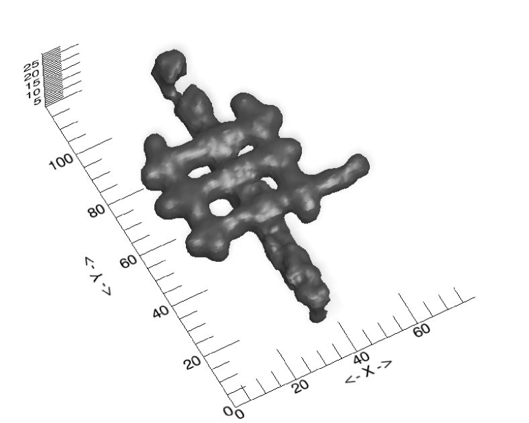
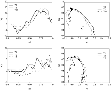
Figure 19.— Morphological templates: crossing filaments forming tunnels (a “forked pattern” in knitting). Left panel: the most complex supercluster template T4. Middle panels: the Minkowski functional $V_{3}$, the right panels—the morphological signature for the templates described in the text. The template number (as in T1) shows the number of tunnels in the model (1, 2 or 4, while 01 denotes a model with one wide tunnel). In all models, one filament is long and thick (the main filament or the body of the supercluster). In the upper panels, other filaments are also long but thin, in the lower panels one more filament is also long (but thin); this filament is crossing the main filament. Other filaments are short (both crossing and parallel).

Fig. 19 shows that in models with tunnels, the value of the 4th Minkowski functional $V_{3}$ becomes negative. The exact value of $V_{3}$ depends also on the number of clumps in the model. The morphological signature $K_{1}$-$K_{2}$ depends on the length of the filaments. Due to too long additional filaments the planarities $K_{1}$ in the upper right panel of Fig. 19 are too large. When additional filaments are short, then the planarities $K_{1}$ are smaller and the morphological signature $K_{1}$-$K_{2}$ of the model is rather similar to that of real superclusters. Such models mimic the superclusters where the rich systems (groups and clusters of galaxies) are connected by fainter systems leaving tunnels between them (as in the supercluster SCl 111) or forming a multibranching filament (as the supercluster SCl 126).

Appendix D Estimating local density distributions for a Cox process

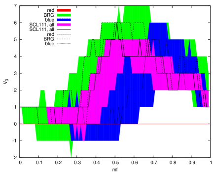
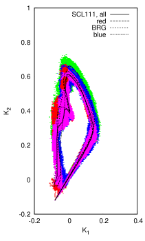
Figure 20.— The 4th Minkowski functional $V_{3}$ (left panel) and the shapefinders $K_{1}$ (planarity) and $K_{2}$ (filamentarity) (right panel) for the red and blue galaxies and the BRGs in the supercluster SCl 111. The black line denotes $V_{3}$ for all galaxies, dashed line with long dashes – for red galaxies, dashed line with short dashes – for BRG-s, and dotted line for blue galaxies. The filled circles in the right panel mark the value of the mass fraction $m_{f}\approx 0.7$. The colored regions show the 95% confidence regions obtained with the shrunk smoothed bootstrap. With red color we show the confidence regions for red galaxies, blue corresponds to blue galaxies, green to BRGs and magenta to the full supercluster.

A popular model for the galaxy distribution is Cox point process (see, e.g. Martínez & Saar, 2002), where galaxies form a Poisson point process with spatially varying intensity, which is given by a realization of a random field. This model has been used successfully to estimate the moments of the galaxy distribution (correlation functions and spectral densities) and to explore their sampling properties. As the spatial density distribution in a finite region is similar to probability distribution, we can use the methods developed to estimate pointwise errors of probability distributions. In case we do not have a model for the distribution, the popular way is to use bootstrap. As is well known, the standard bootstrap – selecting supercluster galaxies randomly with replacement – is not suitable for estimating probability densities, but the smoothed bootstrap is (Silverman & Young, 1987; Davison & Hinkley, 2009). For kernel densities, as used in this paper, the smoothed bootstrap starts as the standard bootstrap by selecting a galaxy (with replacement), but then adding a random shift with the same distribution as the kernel to its coordinates. In order to retain the covariance structure of the density, the shifts are reduced by $(1+h^{2}/\sigma^{2})^{1/2}$, where $h$ is the original kernel width and $\sigma$ is the rms coordinate error for the data (Silverman & Young, 1987). This is called shrunk smoothed bootstrap.

We used such bootstrapped galaxy sample realizations to estimate the confidence regions for the third Minkowski functional $V_{3}$ and for the morphological signature in the $K_{1}$-$K_{2}$ plane. As an example, we show the results in Fig. 20 for the supercluster SCl 111 (1000 realizations; the results for the other two superclusters studied in this paper are similar). We see that the 95% confidence regions are very wide and those for different populations practically overlap, both for $V_{3}$ and for the morphological signature. Does it mean that there is really no inner structure in this supercluster, and no differences in the spatial distribution of different galaxy populations? We see here the evidence that the Cox process model is not good for describing the detailed structure of galaxy associations. It does not account for the scale dependence of the galaxy distribution properties, and a Poisson process clearly cannot describe in full the complex process of galaxy formation that leaves its traces in the final spatial distribution of galaxies. The halo- model based approach used in the main text reflects better the actual observed galaxy distribution.

References

- Abazajian et al. (2009) Abazajian, K. N., et al. 2009, ApJS, 182, 543
- Adelman-McCarthy et al. (2008) Adelman-McCarthy, J. K., et al. 2008, ApJS, 175, 297
- Aragón-Calvo et al. (2010) Aragón-Calvo, M. A., Platen, E., van de Weygaert, R., & Szalay, A. S. 2010, ApJ, 723, 364
- Araya-Melo et al. (2009a) Araya-Melo, P. A., Reisenegger, A., Meza, A., van de Weygaert, R., Dünner, R., & Quintana, H. 2009a, MNRAS, 399, 97
- Araya-Melo et al. (2009b) Araya-Melo, P. A., van de Weygaert, R., & Jones, B. J. T. 2009b, MNRAS, 1458
- Bamford et al. (2009) Bamford, S. P., et al. 2009, MNRAS, 393, 1324
- Bardelli (2004) Bardelli, S. 2004, in IAU Colloq. 195: Outskirts of Galaxy Clusters: Intense Life in the Suburbs, ed. A. Diaferio, 71–77
- Bardelli et al. (2000) Bardelli, S., Zucca, E., Zamorani, G., Moscardini, L., & Scaramella, R. 2000, MNRAS, 312, 540
- Basilakos (2003) Basilakos, S. 2003, MNRAS, 344, 602
- Basilakos et al. (2001) Basilakos, S., Plionis, M., & Rowan-Robinson, M. 2001, MNRAS, 323, 47
- Basilakos et al. (2006) Basilakos, S., Plionis, M., Yepes, G., Gottlöber, S., & Turchaninov, V. 2006, MNRAS, 365, 539
- Belsole et al. (2004) Belsole, E., Pratt, G. W., Sauvageot, J., & Bourdin, H. 2004, A&A, 415, 821
- Benítez et al. (2009) Benítez, N., et al. 2009, ApJ, 691, 241
- Berlind et al. (2006) Berlind, A. A., Kazin, E., Blanton, M. R., Pueblas, S., Scoccimarro, R., & Hogg, D. W. 2006, arXiv:astro-ph/0610524
- Blake et al. (2008) Blake, C., Collister, A., & Lahav, O. 2008, MNRAS, 385, 1257
- Blanton & Roweis (2007) Blanton, M. R., & Roweis, S. 2007, AJ, 133, 734
- Blanton et al. (2003a) Blanton, M. R., et al. 2003a, AJ, 125, 2348
- Blanton et al. (2003b) —. 2003b, ApJ, 592, 819
- Bond et al. (1996) Bond, J. R., Kofman, L., & Pogosyan, D. 1996, Nature, 380, 603
- Bond et al. (2010a) Bond, N. A., Strauss, M. A., & Cen, R. 2010a, MNRAS, 406, 1609
- Bond et al. (2010b) —. 2010b, MNRAS, 409, 156
- Buote et al. (2009) Buote, D. A., Zappacosta, L., Fang, T., Humphrey, P. J., Gastaldello, F., & Tagliaferri, G. 2009, ApJ, 695, 1351
- Choi et al. (2010) Choi, E., Bond, N. A., Strauss, M. A., Coil, A. L., Davis, M., & Willmer, C. N. A. 2010, MNRAS, 406, 320
- Cole et al. (2007) Cole, S., Sánchez, A. G., & Wilkins, S. 2007, in Astronomical Society of the Pacific Conference Series, Vol. 379, Cosmic Frontiers, ed. N. Metcalfe & T. Shanks, 57
- Coles (2009) Coles, P. 2009, in Lecture Notes in Physics, Berlin Springer Verlag, Vol. 665, Lecture Notes in Physics, Berlin Springer Verlag, ed. V. J. Martinez, E. Saar, E. M. Gonzales, & M. J. Pons-Borderia , 493
- Colless et al. (2003) Colless, M., et al. 2003, ArXiv Astrophysics e-prints
- Cooray & Sheth (2002) Cooray, A., & Sheth, R. 2002, Phys. Rep., 372, 1
- Coziol et al. (2009) Coziol, R., Andernach, H., Caretta, C. A., Alamo-Martínez, K. A., & Tago, E. 2009, AJ, 137, 4795
- Croton et al. (2004) Croton, D. J., et al. 2004, MNRAS, 352, 1232
- Davison & Hinkley (2009) Davison, A. C., & Hinkley, D. V. 2009, Bootstrap Methods and Their Application (Cambridge Series in Statistical and Probabilistic Mathematics , No 1) (Cambridge University Press, Cambridge, UK)
- de Lapparent et al. (1986) de Lapparent, V., Geller, M. J., & Huchra, J. P. 1986, ApJ, 302, L1
- Donnelly et al. (2001) Donnelly, R. H., Forman, W., Jones, C., Quintana, H., Ramirez, A., Churazov, E., & Gilfanov, M. 2001, ApJ, 562, 254
- Einasto et al. (2003a) Einasto, J., Hütsi, G., Einasto, M., Saar, E., Tucker, D. L., Müller, V., Heinämäki, P., & Allam, S. S. 2003a, A&A, 405, 425
- Einasto et al. (1984) Einasto, J., Klypin, A. A., Saar, E., & Shandarin, S. F. 1984, MNRAS, 206, 529
- Einasto et al. (2003b) Einasto, J., et al. 2003b, A&A, 410, 425
- Einasto et al. (2006) —. 2006, A&A, 459, L1
- Einasto et al. (2007a) —. 2007a, A&A, 462, 811
- Einasto et al. (2007b) —. 2007b, A&A, 462, 397
- Einasto (1991) Einasto, M. 1991, MNRAS, 252, 261
- Einasto et al. (1994) Einasto, M., Einasto, J., Tago, E., Dalton, G. B., & Andernach, H. 1994, MNRAS, 269, 301
- Einasto et al. (2001) Einasto, M., Einasto, J., Tago, E., Müller, V., & Andernach, H. 2001, AJ, 122, 2222
- Einasto et al. (2003c) Einasto, M., Jaaniste, J., Einasto, J., Heinämäki, P., Müller, V., & Tucker, D. L. 2003c, A&A, 405, 821
- Einasto et al. (2007c) Einasto, M., et al. 2007c, A&A, 464, 815
- Einasto et al. (2007d) —. 2007d, A&A, 476, 697
- Einasto et al. (2008) —. 2008, ApJ, 685, 83
- Einasto et al. (2010) —. 2010, A&A, 522, A92
- Eisenstein et al. (2005a) Eisenstein, D. J., Blanton, M., Zehavi, I., Bahcall, N., Brinkmann, J., Loveday, J., Meiksin, A., & Schneider, D. 2005a, ApJ, 619, 178
- Eisenstein et al. (2001) Eisenstein, D. J., et al. 2001, AJ, 122, 2267
- Eisenstein et al. (2005b) —. 2005b, ApJ, 633, 560
- Erdoğdu et al. (2004) Erdoğdu, P., et al. 2004, MNRAS, 352, 939
- Fleenor & Johnston-Hollitt (2009) Fleenor, M. C., & Johnston-Hollitt, M. 2009, ArXiv e-prints
- Fleenor et al. (2005) Fleenor, M. C., Rose, J. A., Christiansen, W. A., Hunstead, R. W., Johnston-Hollitt, M., Drinkwater, M. J., & Saunders, W. 2005, AJ, 130, 957
- Fleenor et al. (2006) Fleenor, M. C., Rose, J. A., Christiansen, W. A., Johnston-Hollitt, M., Hunstead, R. W., Drinkwater, M. J., & Saunders, W. 2006, AJ, 131, 1280
- Fraley & Raftery (2006) Fraley, C., & Raftery, A. E. 2006, Technical Report, Dep. of Statistics, University of Washington, 504, 1
- Gal et al. (2008) Gal, R. R., Lemaux, B. C., Lubin, L. M., Kocevski, D., & Squires, G. K. 2008, ApJ, 684, 933
- Gaztanaga & Maehoenen (1996) Gaztanaga, E., & Maehoenen, P. 1996, ApJ, 462, L1
- Génova-Santos et al. (2005) Génova-Santos, R., et al. 2005, MNRAS, 363, 79
- Giovanelli et al. (1986) Giovanelli, R., Haynes, M. P., & Chincarini, G. L. 1986, ApJ, 300, 77
- Gott et al. (2005) Gott, J. R. I., Jurić, M., Schlegel, D., Hoyle, F., Vogeley, M., Tegmark, M., Bahcall, N., & Brinkmann, J. 2005, ApJ, 624, 463
- Gott et al. (2008) Gott, J. R. I., et al. 2008, ApJ, 675, 16
- Gregory & Thompson (1978) Gregory, S. A., & Thompson, L. A. 1978, ApJ, 222, 784
- Guzzo et al. (1991) Guzzo, L., Iovino, A., Chincarini, G., Giovanelli, R., & Haynes, M. P. 1991, ApJ, 382, L5
- Haines et al. (2006) Haines, C. P., Merluzzi, P., Mercurio, A., Gargiulo, A., Krusanova, N., Busarello, G., La Barbera, F., & Capaccioli, M. 2006, MNRAS, 371, 55
- Heymans et al. (2008) Heymans, C., et al. 2008, MNRAS, 385, 1431
- Hikage et al. (2003) Hikage, C., et al. 2003, PASJ, 55, 911
- Ho et al. (2009) Ho, S., Lin, Y., Spergel, D., & Hirata, C. M. 2009, ApJ, 697, 1358
- Huchra & Geller (1982) Huchra, J. P., & Geller, M. J. 1982, ApJ, 257, 423
- Hütsi (2006) Hütsi, G. 2006, A&A, 449, 891
- Hwang & Lee (2009) Hwang, H. S., & Lee, M. G. 2009, MNRAS, 397, 2111
- Ihaka & Gentleman (1996) Ihaka, R., & Gentleman, R. 1996, Journal of Computational and Graphical Statistics, 5, 299
- James et al. (2007) James, J. B., Lewis, G. F., & Colless, M. 2007, MNRAS, 375, 128
- Joeveer et al. (1978) Joeveer, M., Einasto, J., & Tago, E. 1978, MNRAS, 185, 357
- Kaldare et al. (2003) Kaldare, R., Colless, M., Raychaudhury, S., & Peterson, B. A. 2003, MNRAS, 339, 652
- Kalinkov & Kuneva (1995) Kalinkov, M., & Kuneva, I. 1995, A&AS, 113, 451
- Kauffmann (1996) Kauffmann, G. 1996, MNRAS, 281, 487
- Kazin et al. (2010) Kazin, E. A., et al. 2010, ApJ, 710, 1444
- Kofman et al. (1987) Kofman, L. A., Einasto, J., & Linde, A. D. 1987, Nature, 326, 48
- Kolokotronis et al. (2002) Kolokotronis, V., Basilakos, S., & Plionis, M. 2002, MNRAS, 331, 1020
- Lietzen et al. (2009) Lietzen, H., et al. 2009, A&A, 501, 145
- Liivamägi et al. (2010) Liivamägi, L. J., Tempel, E., & Saar, E. 2010, ArXiv: 1012.1989
- Lintott et al. (2008) Lintott, C. J., et al. 2008, MNRAS, 389, 1179
- Loeb (2008) Loeb, A. 2008, arXiv:astro-ph/0804.2258
- Malumuth (1992) Malumuth, E. M. 1992, ApJ, 386, 420
- Martínez et al. (2009) Martínez, V. J., Arnalte-Mur, P., Saar, E., de la Cruz, P., Pons-Bordería, M. J., Paredes, S., Fernández-Soto, A., & Tempel, E. 2009, ApJ, 696, L93
- Martínez & Saar (2002) Martínez, V. J., & Saar, E. 2002, Statistics of the Galaxy Distribution (Chapman & Hall/CRC, Boca Raton)
- Masters et al. (2010) Masters, K. L., et al. 2010, MNRAS, 405, 783
- Merritt (1984) Merritt, D. 1984, ApJ, 276, 26
- Mobasher et al. (2005) Mobasher, B., et al. 2005, ApJ, 635, 832
- Moles et al. (2008) Moles, M., et al. 2008, AJ, 136, 1325
- Nakata et al. (2005) Nakata, F., et al. 2005, MNRAS, 357, 1357
- Nichol et al. (2006) Nichol, R. C., et al. 2006, MNRAS, 368, 1507
- Niemi et al. (2007) Niemi, S., Nurmi, P., Heinämäki, P., & Valtonen, M. 2007, MNRAS, 382, 1864
- Ostriker & Tremaine (1975) Ostriker, J. P., & Tremaine, S. D. 1975, ApJ, 202, L113
- Ouchi et al. (2005) Ouchi, M., et al. 2005, ApJ, 620, L1
- Padilla-Torres et al. (2009) Padilla-Torres, C. P., Gutiérrez, C. M., Rebolo, R., Génova-Santos, R., & Rubiño-Martin, J. A. 2009, MNRAS, 396, 53
- Park et al. (2005) Park, C., et al. 2005, ApJ, 633, 11
- Pimbblet (2005) Pimbblet, K. A. 2005, Publications of the Astronomical Society of Australia, 22, 136
- Pimbblet et al. (2004) Pimbblet, K. A., Drinkwater, M. J., & Hawkrigg, M. C. 2004, MNRAS, 354, L61
- Plionis (2004) Plionis, M. 2004, in IAU Colloq. 195: Outskirts of Galaxy Clusters: Intense Life in the Suburbs, ed. A. Diaferio, 19–25
- Porter et al. (2008) Porter, S. C., Raychaudhury, S., Pimbblet, K. A., & Drinkwater, M. J. 2008, MNRAS, 388, 1152
- Proust et al. (2006) Proust, D., et al. 2006, A&A, 447, 133
- Rose et al. (2002) Rose, J. A., Gaba, A. E., Christiansen, W. A., Davis, D. S., Caldwell, N., Hunstead, R. W., & Johnston-Hollitt, M. 2002, AJ, 123, 1216
- Saar (2009) Saar, E. 2009, in Data Analysis in Cosmology, ed. V. J. Martínez & E. Saar & E. Martínez-Gonzalez & M.-J. Pons-Bordería (Springer-Verlag, Berlin), 523–563
- Saar et al. (2007) Saar, E., Martínez, V. J., Starck, J., & Donoho, D. L. 2007, MNRAS, 374, 1030
- Sahni et al. (1998) Sahni, V., Sathyaprakash, B. S., & Shandarin, S. F. 1998, ApJ, 495, L5
- Sathyaprakash et al. (1998) Sathyaprakash, B. S., Sahni, V., & Shandarin, S. 1998, ApJ, 508, 551
- Schmalzing & Buchert (1997) Schmalzing, J., & Buchert, T. 1997, ApJ, 482, L1
- Shandarin et al. (2004) Shandarin, S. F., Sheth, J. V., & Sahni, V. 2004, MNRAS, 353, 162
- Sheth et al. (2003) Sheth, J. V., Sahni, V., Shandarin, S. F., & Sathyaprakash, B. S. 2003, MNRAS, 343, 22
- Silverman (1986) Silverman, B. W. 1986, Density Estimation for Statistics and Data Analysis (Chapman & Hall, CRC Press, Boca Raton)
- Silverman & Young (1987) Silverman, B. W., & Young, G. A. 1987, Biometrika, 74, 469
- Skibba et al. (2009) Skibba, R. A., et al. 2009, MNRAS, 399, 966
- Small et al. (1998) Small, T. A., Ma, C., Sargent, W. L. W., & Hamilton, D. 1998, ApJ, 492, 45
- Stoica et al. (2010) Stoica, R. S., Martínez, V. J., & Saar, E. 2010, A&A, 510, A38
- Swinbank et al. (2007) Swinbank, A. M., et al. 2007, MNRAS, 379, 1343
- Sylos Labini et al. (2009) Sylos Labini, F., Vasilyev, N. L., & Baryshev, Y. V. 2009, A&A, 508, 17
- Tago et al. (2008) Tago, E., Einasto, J., Saar, E., Tempel, E., Einasto, M., Vennik, J., & Müller, V. 2008, A&A, 479, 927
- Tago et al. (2010) Tago, E., Saar, E., Tempel, E., Einasto, J., Einasto, M., Nurmi, P., & Heinämäki, P. 2010, A&A, 514, A102
- Tanaka et al. (2009) Tanaka, M., Finoguenov, A., Kodama, T., Koyama, Y., Maughan, B., & Nakata, F. 2009, A&A, 505, L9
- Tempel et al. (2009) Tempel, E., Einasto, J., Einasto, M., Saar, E., & Tago, E. 2009, A&A, 495, 37
- Tinker et al. (2010) Tinker, J. L., Wechsler, R. H., & Zheng, Z. 2010, ApJ, 709, 67
- Tovmassian & Plionis (2009) Tovmassian, H. M., & Plionis, M. 2009, ApJ, 696, 1441
- Turner & Gott (1976) Turner, E. L., & Gott, III, J. R. 1976, ApJS, 32, 409
- van de Weygaert et al. (2009) van de Weygaert, R., Aragon-Calvo, M. A., Jones, B. J. T., & Platen, E. 2009, ArXiv: 0912.3448
- van de Weygaert & Schaap (2009) van de Weygaert, R., & Schaap, W. 2009, in Lecture Notes in Physics, Berlin Springer Verlag, Vol. 665, Lecture Notes in Physics, Berlin Springer Verlag, ed. V. J. Martinez, E. Saar, E. M. Gonzales, & M. J. Pons-Borderia , 291
- van den Bosch et al. (2008) van den Bosch, F. C., Pasquali, A., Yang, X., Mo, H. J., Weinmann, S., McIntosh, D. H., & Aquino, D. 2008, ArXiv: 0805.0002
- van den Bosch et al. (2007) van den Bosch, F. C., et al. 2007, MNRAS, 376, 841
- Venemans et al. (2004) Venemans, B. P., et al. 2004, A&A, 424, L17
- Vogeley et al. (2004) Vogeley, M. S., Hoyle, F., Rojas, R. R., & Goldberg, D. M. 2004, in IAU Colloq. 195: Outskirts of Galaxy Clusters: Intense Life in the Suburbs, ed. A. Diaferio, 5–11
- Wang et al. (2008) Wang, Y., Yang, X., Mo, H. J., van den Bosch, F. C., Weinmann, S. M., & Chu, Y. 2008, ApJ, 687, 919
- Watson et al. (2010) Watson, D. F., Berlind, A. A., McBride, C. K., & Masjedi, M. 2010, ApJ, 709, 115
- Wolf et al. (2005) Wolf, C., Gray, M. E., & Meisenheimer, K. 2005, A&A, 443, 435
- Yamila Yaryura et al. (2010) Yamila Yaryura, C., Baugh, C. M., & Angulo, R. E. 2010, ArXiv: 1003.4259
- Yang et al. (2008) Yang, X., Mo, H. J., & van den Bosch, F. C. 2008, ApJ, 676, 248
- Yang et al. (2005) Yang, X., Mo, H. J., van den Bosch, F. C., & Jing, Y. P. 2005, MNRAS, 356, 1293
- Yang et al. (2007) Yang, X., Mo, H. J., van den Bosch, F. C., Pasquali, A., Li, C., & Barden, M. 2007, ApJ, 671, 153
- Zappacosta et al. (2005) Zappacosta, L., Maiolino, R., Finoguenov, A., Mannucci, F., Gilli, R., & Ferrara, A. 2005, A&A, 434, 801
- Zehavi et al. (2002) Zehavi, I., et al. 2002, ApJ, 571, 172
- Zehavi et al. (2005) —. 2005, ApJ, 621, 22
- Zehavi, I. and the SDSS Collaboration et al. (2010) Zehavi, I. and the SDSS Collaboration et al. 2010, ArXiv: 1005.2413
- Zeldovich et al. (1982) Zeldovich, I. B., Einasto, J., & Shandarin, S. F. 1982, Nature, 300, 407
- Zheng et al. (2008) Zheng, Z., Zehavi, I., Eisenstein, D. J., Weinberg, D. H., & Jing, Y. P. 2008, ArXiv: 0809.1868
- Zucca et al. (1993) Zucca, E., Zamorani, G., Scaramella, R., & Vettolani, G. 1993, ApJ, 407, 470