Extended quantum $U(1)$-liquid phase in a three-dimensional quantum dimer model

Abstract

Recently, quantum dimer models have attracted a great deal of interest as a paradigm for the study of exotic quantum phases. Much of this excitement has centred on the claim that a certain class of quantum dimer model can support a quantum $U(1)$ liquid phase with deconfined fractional excitations in three dimensions. These fractional monomer excitations are quantum analogues of the magnetic monopoles found in spin ice. In this article we use extensive quantum Monte Carlo simulations to establish the ground-state phase diagram of the quantum dimer model on the three-dimensional diamond lattice as a function of the ratio $\mu$ of the potential to kinetic energy terms in the Hamiltonian. We find that, for $\mu_{c}=0.75\pm 0.02$, the model undergoes a first-order quantum phase transition from an ordered “R-state” into an extended quantum $U(1)$ liquid phase, which terminates in a quantum critical “RK point” for $\mu=1$. This confirms the published field-theoretical scenario. We present detailed evidence for the existence of the $U(1)$ liquid phase, and indirect evidence for the existence of its photon and monopole excitations. Simulations are benchmarked against a variety of exact and perturbative results, and a comparison is made of different variational wave functions. We also explore the ergodicity of the quantum dimer model on a diamond lattice within a given flux sector, identifying a new conserved quantity related to transition graphs of dimer configurations. These results complete and extend the analysis previously published in [O. Sikora et al. Phys. Rev. Lett. 103, 247001 (2009)].

I Introduction

Dimer models, which describe the myriad possible configurations of hard-core objects on bonds, have long been a touch-stone of statistical mechanics fisher61 ; kastelyn61 . Quantum dimer models (QDM’s), in which dimers are allowed to resonate between different degenerate configurations, were first introduced to describe antiferromagnetic correlations in high-$T_{c}$ superconductors rokhsar88 . It has since been realized that QDM’s arise naturally as effective models of many different condensed matter systems, and provide a concrete realizations of several classes of lattice gauge theories. As such, they have become central to the theoretical search for new quantum phases and excitations. A key question in this context is when, if ever, a QDM can support a liquid ground state?

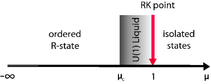
Figure 1: (Color online) Phase diagram of the quantum dimer model on a diamond lattice, as a function of the ratio $\mu$ of potential to kinetic energy, following moessner03 ; bergman06-PRB ; sikora09 .

The answer to this question depends on lattice dimension and topology. In two dimensions (2D), the situation is relatively well-understood diep04 , and a liquid ground state is known to exist in the QDM on the non-bipartite triangular moessner01 and kagome misguich02 lattices. This liquid is gapped and has deconfined fractional excitations, which are vortices of an underlying $\mathbb{Z}_{2}$ (Ising) gauge theory. Meanwhile, for 2D bipartite lattices, the underlying gauge theory has a $U(1)$ character, akin to electromagnetism huse03 ; moessner03 . In this case a liquid state is found only at a single, critical, “Rokhsar-Kivelson” (RK) point rokhsar88 . Away from this, the system crystallizes into phases with broken lattice symmetries. For the QDM on a square lattice, these are columnar dimer and resonating plaquette phases leung96 ; trousselet08 . A very similar phase diagram is found for the QDM on a honeycomb lattice moessner01-honeycomb .

Much less is known about QDM’s in three dimensions (3D). However here field theoretical arguments suggest that a new, extended $U(1)$-liquid phase with gapless photon-like excitations might “grow” out of the RK point for a 3D QDM on a bipartite lattice moessner03 ; bergman06-PRB (see Fig. 1). Similar claims have been made for the closely related quantum loop model in three dimensions hermele04 .

In a recent Letter sikora09 , we presented numerical evidence for the existence of an extended quantum $U(1)$ liquid phase with deconfined fractional excitations in a three-dimensional QDM, taken directly from its microscopic Hamiltonian. We considered the specific example of a QDM on a diamond lattice, which may serve as an effective model for the frustration found in various spinel compounds bergman06-PRB ; fulde02 . From zero-temperature GFMC simulations of clusters of up to $2000$ sites we were able to demonstrate the existence of a quantum $U(1)$-liquid phase for a range of parameters $0.77\pm 0.02<\mu<1$ bordering on the RK point [cf. Fig. 1]. These results complement a recent finite-temperature quantum Monte Carlo study of a microscopic model of interacting bosons which can be mapped onto an effective quantum loop model banerjee08 .

In this article we document the evidence for these claims, taken from explicit calculations of (i) the order parameter of the competing (dimer)-ordered phase [cf. Fig. 2], (ii) the “string tension” associated with fractional monomer excitations and (iii) the finite-size scaling of a characteristic set of energy gaps associated with the U(1) liquid phase. We also explore the internal consistency of these calculations, cross-checking simulations against exact diagonalization of small clusters and perturbative expansions about exactly soluble limits of the model.

We pay particular attention to the thorny question of the ergodicity of GFMC simulations in the presence of hidden quantum numbers. In the 2D QDM’s studied previously, the quantum numbers are well understood, and it is clear which dimer configurations are connected by the QDM Hamiltonian. This is not, however, the case for the 3D QDM considered in this article. Despite the fact that we can define a “magnetic” flux $\vec{\phi}$ which is a good quantum number — in a manner similar to the square-lattice QDM in 2D — the QDM Hamiltonian on a diamond lattice connects only sub-sets of dimer configurations within of each flux sector. This means that the QDM on diamond lattice is not ergodic within a given flux sector, and great care must be taken to ensure that simulations accurately represent the true ground state for each value of flux $\vec{\phi}$. We shed some light on this issue by identifying a new, hidden, quantum number conserved by the QDM on diamond lattice.

The paper is structured as follows :

In Section II we introduce the model and summarize the properties of the proposed $U(1)$-liquid phase. We demonstrate a way of constructing dimer configurations with different values of magnetic flux, and define an order parameter for the ordered “R-state” found for negative values of $\mu$. In Section III we use Green’s function Monte Carlo simulations to obtain explicit predictions for the $\mu$ dependence of the order parameter, monomer string tension and ground state energy as a function of magnetic flux for a range of different cluster sizes and geometries. We confirm the conjectured form of the phase diagram Fig. 1, and use careful finite size scaling to obtain an improved estimate of the location of the phase transition from ordered to liquid phases in the thermodynamic limit as $\mu_{c}=0.75\pm 0.02$. In Section IV, we explore the ergodicity of our simulations within a given flux sector and confirm that the techniques used give reliable estimates of ground state properties. We also identify an additional $\mathbb{Z}_{2}$ quantum number which divides each flux sector into two distinct parts. In Section V we summarise our results and briefly discuss remaining open issues.

The paper concludes with some technical appendices. In Appendix A we discuss the generalization to a fermionic QDM and show that it is equivalent to the bosonic case in lowest order. In Appendix B we exhibit a Landau theory for the ordered, R-state. In Appendix C we compare different variational wave functions, and use these to investigate the transition from ordered to liquid ground states. In Appendix D we benchmark our Green’s function Monte Carlo simulations against perturbation theory about exactly soluble limits of the model.

II The Quantum Dimer Model and what you need to know about it

II.1 The model and its derivation

In the spirit of Ref. rokhsar88, , we study the quantum dimer model (QDM)

$${\mathcal{H}}_{\sf QDM}=-g{\mathcal{K}}_{\sf f}+\mu{\mathcal{N}}_{\sf f}$$ (1)

where the matrix elements of

$${\mathcal{K}}_{\sf f} = \sum_{\;\pspicture(0.0pt,2.84526pt)(5.69054pt,8.53581pt)\psset{linewidth=0.85358pt,linestyle=solid}{\psset{}\pspolygon(0.0pt,2.20508pt)(0.0pt,6.40186pt)(3.52814pt,8.53581pt)(7.25545pt,6.40186pt)(7.25545pt,2.20508pt)(3.52814pt,0.0pt)}\endpspicture\;}\left(\Big{|}\;\pspicture(0.0pt,2.84526pt)(9.95845pt,17.07164pt)\psset{unit=21.33957pt}{\pspolygon(0.0pt,3.20093pt)(0.0pt,9.6028pt)(5.544pt,12.80374pt)(11.08803pt,9.6028pt)(11.08803pt,3.20093pt)(5.544pt,0.0pt)}\psset{linewidth=2.56075pt,linestyle=solid}{\psline(0.0pt,3.20093pt)(0.0pt,9.6028pt)}{\psline(5.544pt,12.80374pt)(11.08803pt,9.6028pt)}{\psline(11.08803pt,3.20093pt)(5.544pt,0.0pt)}\endpspicture\;\Big{\rangle}\Big{\langle}\;\pspicture(0.0pt,2.13396pt)(7.46884pt,12.80374pt)\psset{unit=21.33957pt}\psset{linewidth=0.64018pt,linestyle=solid}{\psset{}\pspolygon(0.0pt,3.20093pt)(0.0pt,9.6028pt)(5.544pt,12.80374pt)(11.08803pt,9.6028pt)(11.08803pt,3.20093pt)(5.544pt,0.0pt)}\psset{linewidth=2.56075pt,linestyle=solid}{\psline(5.544pt,12.80374pt)(0.0pt,9.6028pt)}{\psline(11.08803pt,2.56075pt)(11.08803pt,9.6028pt)}{\psline(5.544pt,0.0pt)(0.0pt,3.20093pt)}\endpspicture\;\Big{|}+\Big{|}\;\pspicture(0.0pt,2.13396pt)(7.46884pt,12.80374pt)\psset{unit=21.33957pt}\psset{linewidth=0.64018pt,linestyle=solid}{\psset{}\pspolygon(0.0pt,3.20093pt)(0.0pt,9.6028pt)(5.544pt,12.80374pt)(11.08803pt,9.6028pt)(11.08803pt,3.20093pt)(5.544pt,0.0pt)}\psset{linewidth=2.56075pt,linestyle=solid}{\psline(5.544pt,12.80374pt)(0.0pt,9.6028pt)}{\psline(11.08803pt,2.56075pt)(11.08803pt,9.6028pt)}{\psline(5.544pt,0.0pt)(0.0pt,3.20093pt)}\endpspicture\;\Big{\rangle}\Big{\langle}\;\pspicture(0.0pt,2.13396pt)(7.46884pt,12.80374pt)\psset{unit=21.33957pt}{\pspolygon(0.0pt,3.20093pt)(0.0pt,9.6028pt)(5.544pt,12.80374pt)(11.08803pt,9.6028pt)(11.08803pt,3.20093pt)(5.544pt,0.0pt)}\psset{linewidth=2.56075pt,linestyle=solid}{\psline(0.0pt,3.20093pt)(0.0pt,9.6028pt)}{\psline(5.544pt,12.80374pt)(11.08803pt,9.6028pt)}{\psline(11.08803pt,3.20093pt)(5.544pt,0.0pt)}\endpspicture\;\Big{|}\right)$$ (2)

connect different, degenerate dimer configurations by cyclically permuting dimers on six-bond “flippable” plaquettes of alternating filled and empty links within the diamond lattice [cf. Fig. 2], while

$${\mathcal{N}}_{f} = \sum_{\;\pspicture(0.0pt,2.84526pt)(5.69054pt,8.53581pt)\psset{linewidth=0.85358pt,linestyle=solid}{\psset{}\pspolygon(0.0pt,2.20508pt)(0.0pt,6.40186pt)(3.52814pt,8.53581pt)(7.25545pt,6.40186pt)(7.25545pt,2.20508pt)(3.52814pt,0.0pt)}\endpspicture\;}\left(\Big{|}\;\pspicture(0.0pt,2.84526pt)(9.95845pt,17.07164pt)\psset{unit=21.33957pt}{\pspolygon(0.0pt,3.20093pt)(0.0pt,9.6028pt)(5.544pt,12.80374pt)(11.08803pt,9.6028pt)(11.08803pt,3.20093pt)(5.544pt,0.0pt)}\psset{linewidth=2.56075pt,linestyle=solid}{\psline(0.0pt,3.20093pt)(0.0pt,9.6028pt)}{\psline(5.544pt,12.80374pt)(11.08803pt,9.6028pt)}{\psline(11.08803pt,3.20093pt)(5.544pt,0.0pt)}\endpspicture\;\Big{\rangle}\Big{\langle}\;\pspicture(0.0pt,2.13396pt)(7.46884pt,12.80374pt)\psset{unit=21.33957pt}{\pspolygon(0.0pt,3.20093pt)(0.0pt,9.6028pt)(5.544pt,12.80374pt)(11.08803pt,9.6028pt)(11.08803pt,3.20093pt)(5.544pt,0.0pt)}\psset{linewidth=2.56075pt,linestyle=solid}{\psline(0.0pt,3.20093pt)(0.0pt,9.6028pt)}{\psline(5.544pt,12.80374pt)(11.08803pt,9.6028pt)}{\psline(11.08803pt,3.20093pt)(5.544pt,0.0pt)}\endpspicture\;\Big{|}+\Big{|}\;\pspicture(0.0pt,2.13396pt)(7.46884pt,12.80374pt)\psset{unit=21.33957pt}\psset{linewidth=0.64018pt,linestyle=solid}{\psset{}\pspolygon(0.0pt,3.20093pt)(0.0pt,9.6028pt)(5.544pt,12.80374pt)(11.08803pt,9.6028pt)(11.08803pt,3.20093pt)(5.544pt,0.0pt)}\psset{linewidth=2.56075pt,linestyle=solid}{\psline(5.544pt,12.80374pt)(0.0pt,9.6028pt)}{\psline(11.08803pt,2.56075pt)(11.08803pt,9.6028pt)}{\psline(5.544pt,0.0pt)(0.0pt,3.20093pt)}\endpspicture\;\Big{\rangle}\Big{\langle}\;\pspicture(0.0pt,2.13396pt)(7.46884pt,12.80374pt)\psset{unit=21.33957pt}\psset{linewidth=0.64018pt,linestyle=solid}{\psset{}\pspolygon(0.0pt,3.20093pt)(0.0pt,9.6028pt)(5.544pt,12.80374pt)(11.08803pt,9.6028pt)(11.08803pt,3.20093pt)(5.544pt,0.0pt)}\psset{linewidth=2.56075pt,linestyle=solid}{\psline(5.544pt,12.80374pt)(0.0pt,9.6028pt)}{\psline(11.08803pt,2.56075pt)(11.08803pt,9.6028pt)}{\psline(5.544pt,0.0pt)(0.0pt,3.20093pt)}\endpspicture\;\Big{|}\right)$$ (3)

counts the number of such flippable plaquettes. In what follows we will consider $g>0$, with $-\infty<\mu\leq g$.

This QDM Hamiltonian acts on the $\approx 1.3^{N/2}$ different dimer configurations which cover the links the $N$-bond diamond lattice nagle66 . This Hilbert space breaks up into different subsectors $\lambda_{\sf c}$, defined by the sets of dimer configurations which are connected by the matrix elements of ${\mathcal{K}}_{\sf f}$. The number and nature of these subsectors remains an open problem, which will be discussed at length in Section IV of this article.

Crucially, however, all off-diagonal matrix elements of Eq. (1) are zero or negative. By the Frobenius-Perron theorem, the lowest energy state of the QDM within any given subsector of the Hilbert space $\lambda_{\sf c}$ must then be a nodeless superposition of dimer configurations

$$\mid\psi_{0}\rangle_{\lambda_{\sf c}}=\sum_{{\sf c}\in\lambda_{\sf c}}a_{\sf c}|{\sf c}\rangle$$ (4)

with real, positive coefficients $a_{\sf c}$. As a result, Quantum Monte Carlo simulations of Eq. (1) are not subject to a sign problem.

Exactly at the RK point $\mu=g$, the QDM Hamiltonian can be written as a sum of projectors

$${\mathcal{H}}_{RK} = g\sum_{\;\pspicture(0.0pt,2.84526pt)(5.69054pt,8.53581pt)\psset{linewidth=0.85358pt,linestyle=solid}{\psset{}\pspolygon(0.0pt,2.20508pt)(0.0pt,6.40186pt)(3.52814pt,8.53581pt)(7.25545pt,6.40186pt)(7.25545pt,2.20508pt)(3.52814pt,0.0pt)}\endpspicture\;}\left[\Big{|}\;\pspicture(0.0pt,2.84526pt)(9.95845pt,17.07164pt)\psset{unit=21.33957pt}{\pspolygon(0.0pt,3.20093pt)(0.0pt,9.6028pt)(5.544pt,12.80374pt)(11.08803pt,9.6028pt)(11.08803pt,3.20093pt)(5.544pt,0.0pt)}\psset{linewidth=2.56075pt,linestyle=solid}{\psline(0.0pt,3.20093pt)(0.0pt,9.6028pt)}{\psline(5.544pt,12.80374pt)(11.08803pt,9.6028pt)}{\psline(11.08803pt,3.20093pt)(5.544pt,0.0pt)}\endpspicture\;\Big{\rangle}-\Big{|}\;\pspicture(0.0pt,2.13396pt)(7.46884pt,12.80374pt)\psset{unit=21.33957pt}\psset{linewidth=0.64018pt,linestyle=solid}{\psset{}\pspolygon(0.0pt,3.20093pt)(0.0pt,9.6028pt)(5.544pt,12.80374pt)(11.08803pt,9.6028pt)(11.08803pt,3.20093pt)(5.544pt,0.0pt)}\psset{linewidth=2.56075pt,linestyle=solid}{\psline(5.544pt,12.80374pt)(0.0pt,9.6028pt)}{\psline(11.08803pt,2.56075pt)(11.08803pt,9.6028pt)}{\psline(5.544pt,0.0pt)(0.0pt,3.20093pt)}\endpspicture\;\Big{\rangle}\right]\left[\Big{\langle}\;\pspicture(0.0pt,2.84526pt)(9.95845pt,17.07164pt)\psset{unit=21.33957pt}{\pspolygon(0.0pt,3.20093pt)(0.0pt,9.6028pt)(5.544pt,12.80374pt)(11.08803pt,9.6028pt)(11.08803pt,3.20093pt)(5.544pt,0.0pt)}\psset{linewidth=2.56075pt,linestyle=solid}{\psline(0.0pt,3.20093pt)(0.0pt,9.6028pt)}{\psline(5.544pt,12.80374pt)(11.08803pt,9.6028pt)}{\psline(11.08803pt,3.20093pt)(5.544pt,0.0pt)}\endpspicture\;\Big{|}-\Big{\langle}\;\pspicture(0.0pt,2.13396pt)(7.46884pt,12.80374pt)\psset{unit=21.33957pt}\psset{linewidth=0.64018pt,linestyle=solid}{\psset{}\pspolygon(0.0pt,3.20093pt)(0.0pt,9.6028pt)(5.544pt,12.80374pt)(11.08803pt,9.6028pt)(11.08803pt,3.20093pt)(5.544pt,0.0pt)}\psset{linewidth=2.56075pt,linestyle=solid}{\psline(5.544pt,12.80374pt)(0.0pt,9.6028pt)}{\psline(11.08803pt,2.56075pt)(11.08803pt,9.6028pt)}{\psline(5.544pt,0.0pt)(0.0pt,3.20093pt)}\endpspicture\;\Big{|}\right]$$ (5)

In this case the ground state in any subsector of the Hilbert space $\lambda_{\sf c}$ is the zero-energy eigenstate given by the equally weighted sum over all dimer configurations within that subsector.

$$|{\sf RK}\rangle_{\lambda_{\sf c}}\propto\sum_{{\sf c}\in\lambda_{\sf c}}|{\sf c}\rangle$$ (6)

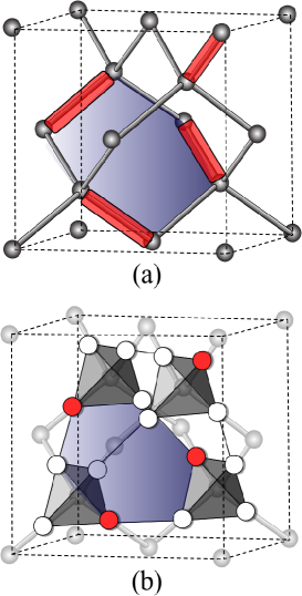
Figure 2: (Color online) (a) Cubic unit cell of the diamond lattice, with bonds occupied by dimers shown by thick red links. The dimer configuration shown is the ordered “R-state” found for negative $\mu$. This contains a “flippable” hexagonal plaquette, which is shaded blue. (b) Equivalent cubic unit cell of the pyrochlore lattice, with sites occupied by hard-core bosons shown in red. The boson configuration shown is the same ordered “R-state”.

The QDM Eq. (1) can be derived from various microscopic models. One example is a hard-core boson model on a pyrochlore lattice formed of corner sharing tetrahedra

$${\mathcal{H}}_{\sf tV}=-t\sum_{\langle ij\rangle}(b_{i}^{\dagger}b_{j}+H.c.)+V\sum_{\langle ij\rangle}n_{i}n_{j}$$ (7)

at quarter filling, in the limit of large nearest-neighbor interactions $V\gg t$. In this case, the low energy configurations are those without bosons on neighbouring sites. This imposes the constraint of placing exactly one boson in each tetrahedron.

The diamond lattice is the medial lattice of the pyrochlore lattice, formed by connecting the centres of all tetrahedra (see Fig. 2), and and these constrained states are in exact one-to-one correspondence with the dimer coverings of a diamond lattice. The lowest-order process in degenerate perturbation theory which connects these states is a cyclic exchange of bosons around the smallest, hexagonal plaquette of the pyrochlore lattice. This occurs at third order in the hopping of bosons, giving $g=12t^{3}/V^{2}$.

Another physically motivated model which reduces to the quantum dimer model on the diamond lattice is the easy-axis quantum antiferromagnet on a pyrochlore lattice

$${\mathcal{H}}_{\sf XXZ}=J_{xy}\sum_{\langle ij\rangle}(S^{x}_{i}S^{x}_{j}+S^{y}_{i}S^{y}_{j})+J_{z}\sum_{\langle ij\rangle}S^{z}_{i}S^{z}_{j}$$

$$-h\sum_{i}S^{z}_{i}$$ (8)

at half-magnetization $\langle S^{z}\rangle\equiv S/2$. For $S=1/2$ this is exactly equivalent to the hard-core boson problem considered above, with each occupied site corresponding to a “up” spin, and each empty site to a “down” spin, with the caveat that the kinetic energy term $J_{xy}$ now has the opposite sign, and so $g=-12J_{xy}^{3}/J_{z}^{2}$.

At first sight this might seem to imply that the $XXZ$ model Eq. (II.1) with $g<0$ has a different ground state from the a $t$-$V$ model with $g>0$ Eq. (7). However the global sign of $g$ can be changed by the simple unitary transformation

$$|c\rangle\rightarrow\exp[i\pi{\mathcal{N}_{\Lambda}}/2]|c\rangle$$ (9)

where $|c\rangle$ is an arbitrary dimer configuration and $\mathcal{N}_{\Lambda}$ counts the number of dimers which occupy the subset of diamond lattice bonds $\Lambda$ shown in Fig. 3. The cyclic permutation of dimers on any six-bond flippable plaquette changes $\mathcal{N}_{\Lambda}$ by two, and so the unitary transformation Eq. (9) maps $g\to-g$. Moreover, exactly the same quantum dimer model Eq. (1) can be derived from a fermionic $t$-$V$ model, i.e. Eq. (7) with Fermi operators substituted for the bosonic ones. This mapping is described in Appendix A.

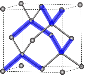
Figure 3: (Color online) The subset of diamond lattice bonds $\Lambda$ (thick, blue, shaded bonds) used in the unitary transformation Eq. (9) which maps $g\to-g$ in Eq. (1).

An effective Hamiltonian of the QDM form Eq. (1) can also be derived from Eq. (II.1) for larger values of spin. For $S=3/2$, where the model might be of relevance to Cr spinels, this was accomplished by Bergman et al. bergman06-PRL , who found $\mu/g\approx-7$. A two-dimensional analogue of Eq. (1) might also be realized using cold atoms ruostekoski09 . Finally, quantum dimer models also arise as effective models of spin–orbital models vernay06 .

Since the goal of this paper is to determine the ground state phases of Eq. (1), and not to relate it to any particular physical system, in what follows we set $g=1$, and study the model as a function of the single adjustable parameter $\mu$. For $\mu\rightarrow-\infty$ the potential energy dominates, and the ground state of Eq. (1) is the set of dimer configurations which maximise the number of “flippable” hexagons, with one out of four hexagons being flippable. This is the so-called R-state bergman06-PRL , illustrated in Fig. 2, which has a cubic unit cell and is eight-fold degenerate.

At the RK point $\mu=1$, the ground state is the equally weighted sum of all possible dimer configurations rokhsar88 , while for $\mu>1$, ground states are the many “isolated states” which contain no flippable hexagons, and so have no kinetic energy. The interest of the QDM therefore rests in the parameter range $-1\lesssim\mu\leq 1$, for which kinetic and potential energy compete on an equal footing. It is this range of parameters which we consider below.

II.2 Effective electrodynamics

For purpose of comparison with numerics, we now briefly review the field theory arguments underlying the proposed $U(1)$ liquid phase. The defining property of a dimer model is that every lattice site is touched by exactly one dimer. The diamond lattice is bipartite — we can divide it in two sublattices, $A$ and $B$, such that every every link (bond) of the lattice connects an $A$ sublattice site with a $B$ sublattice site. We can use this property to associate a magnetic flux vector ${\bf B}$ with each bond of the lattice. Bonds not occupied by a dimer are assigned one (arbitrary) unit of magnetic flux, directed from $B$ to $A$. Where a dimer is present, we assign three units of flux to that bond, directed from $A$ to $B$ .

In this language, the constraint that every lattice site is touched by one dimer becomes the condition

$$\nabla\cdot\mathbf{B}=0.$$ (10)

We resolve this constraint by writing

$$\mathbf{B}=\mathbf{\nabla}\times\mathbf{A},$$ (11)

where the gauge field $\mathbf{A}$ is defined on the sites of the original diamond lattice while the fictitious magnetic field $\mathbf{B}$ is defined on its bonds. We chose to work in the Coulomb gauge $\nabla\cdot\mathbf{A}=0$. In the absence of quantum effects, the statistical description of the dimer model reduces to a relatively straightforward problem in magnetostatics, and the ground state of the dimer model is found to be classical $U(1)$-liquid. Correlations between dimers have a dipolar form in real space, and the constraint $\nabla\cdot\mathbf{B}=0$ manifests itself as a set of “pinch points” in the structure factor in k-space youngblood80 ; huse03 ; henley05 ; isakov06 ; henley10 . Exactly this situation is realized in the rare-earth magnet spin ice fennel09 .

The purpose of this paper is to treat the quantum effects which arise from the tunnelling of the system from one dimer configuration to another, as described by Eq. (1). This tunnelling introduces fluctuations in time of the gauge field $\mathbf{A}$, which in turn give rise to an effective electric field

$$\mathbf{E}=-\partial_{t}\mathbf{A}.$$ (12)

None the less, the total magnetic flux $\phi=\int d{\mathbf{S}}\cdot{\mathbf{B}}$ through any plane in the lattice remains a conserved quantity, since the dynamics present in the quantum dimer model only permit a reversal in the sense of flux around a closed loop.

This representation clearly has a lot in common with conventional electromagnetism and, following Ref. moessner03, , we can use this analogy to write down a plausible long-wavelength action for the QDM on a diamond lattice

$$\mathcal{S}=\int d^{3}xdt\left[\mathbf{E}^{2}-c^{2}\mathbf{B}^{2}\right],$$ (13)

where $c^{2}>0$. This is the Maxwell action of conventional electromagnetism, and the system must posses linearly dispersing “photons” (transverse excitations of the gauge field ${\bf A}$) with speed of light $c$. These conditions were argued to be realized in a quantum $U(1)$-liquid state bordering the RK point in three-dimensional quantum dimer models on a bipartite lattice for $\mu\lesssim 1$ [moessner03, ], leading to the conjectured phase diagram Fig. 1. An exactly parallel story can be told about the quantum loop model in three dimensions hermele04 .

These “emergent” photons are the signature feature of the proposed $U(1)$-liquid state, and offer a beautiful realization of Maxwell’s laws in a condensed matter system. However, for the purposes of this study, we wish to emphasize that Eq. (13) also contains information about the finite size scaling of the energy spectra. A flux $\phi$ through a cluster of volume $L^{3}$ corresponds to an average magnetic field $B=\phi/L^{2}$. In the $U(1)$-liquid state, this magnetic field is uniformly distributed on the “coarse-grained” scale of the effective action Eq. (13). It then follows from Eq. (13) that the energy difference $\Delta_{\phi}=E_{\phi}-E_{0}$ between the ground state of the zero-flux sector, and the lowest energy state of the sector with flux $\phi$ scales as

$$\Delta_{\phi}=E_{\phi}-E_{0}=c^{2}\frac{\phi^{2}}{L}\ .$$ (14)

In the thermodynamic limit $\Delta_{\phi}\to 0$ and different flux sectors should be treated as degenerate ground states. A second finite-size prediction of Eq. (13) is that the ground state energy of the $U(1)$-liquid state should have a finite size correction $\Delta E$ from the zero-point energy of photons which in leading order scales as

$$\frac{\Delta E(L)}{N}\sim\left[\int_{\frac{2\pi}{L}}^{\Lambda^{\prime}}dk-\int_{0}^{\Lambda^{\prime}}dk\right]k^{2}ck\sim-\frac{c}{L^{4}}$$ (15)

where $\Lambda^{\prime}$ is a size-independent momentum cutoff. In this paper we make use of both Eq. (14) and Eq. (15) to study finite size properties of Eq. (1).

II.3 Clusters used in simulation

Our evidence for the existence of a quantum $U(1)$-liquid phase is taken from simulation of the quantum dimer model Eq. (1) on finite-size clusters of the diamond lattice with periodic boundary conditions. For the size of a cluster use the notation in which $N$ is the number of pyrochlore lattice sites, corresponding to the diamond lattice bonds. The periodic boundary conditions permit us to associate a set of (integer) topological quantum numbers $\vec{\phi}=(\phi_{1},\phi_{2},\phi_{3})$ with the flux through a set of orthogonal planes. This reduces the Hilbert space of the problem from the $\approx 1.3^{N/2}$ different dimer configurations to a set of discrete sectors with given $\vec{\phi}$.

An important lesson from the exact diagonalization of small clusters is that the matrix elements of Eq. (1) do not connect all dimer configurations within a given value of $\vec{\phi}$. None the less, the size of the largest blocks is still too large to permit the exact diagonalization of clusters with more that 128 diamond lattice bonds. These clusters are very small by the standards of the (implicitly) course-grained field theory Eq. (13), and quantum Monte Carlo simulations must therefore be used to determine the ground state of the model.

Table 1: Cluster geometries used in simulations. The first column gives the short notation for cluster geometry used in the text; the second column, the number of diamond lattice bonds; the last three columns show the vectors ${\bf g}_{i}$ which define the translation vectors of the cluster. The integer $l$ defines the size of the cluster, within a given family. The [100] clusters have side of length of $L=2l$, and contain $N=2L^{3}$ bonds.

	number of bonds	${\bf g}_{1}$	${\bf g}_{2}$	${\bf g}_{3}$
$[$100$]$	$16\,l^{3}$	$2l\,(1,0,0)$	$2l\,(0,1,0)$	$2l\,(0,0,1)$
$[$110$]$	$32\,l^{3}$	$2l\,(1,1,0)$	$2l\,(0,1,1)$	$2l\,(1,0,1)$
$[$111$]$	$64\,l^{3}$	$2l\,(1,1,-1)$	$2l\,(1,-1,1)$	$2l\,(-1,1,1)$

The quantum Monte Carlo method we chose is GFMC (Green’s function Monte Carlo), which constructs Monte Carlo updates using only the Hamiltonian dynamics of Eq. (1). This has the advantage that all quantum numbers (including magnetic flux) are preserved in simulation. However since not all of these quantum numbers are known a priori, great care must be taken to simulate in the appropriate subsectors of the Hilbert space. This is an issue which we discuss at length in Section IV. Moreover, because an exponential number of dimer configurations contribute to the ground state wave function of the $U(1)$-liquid, quantum Monte Carlo simulations are themselves limited to clusters of up to 2000 diamond lattice bonds.

In order to gain the most from finite size scaling, we therefore consider a range of different cluster geometries. We restrict ourselves to clusters which are compatible with the 16-bond unit cell of the R-state, and group them into families of clusters with the same shape. These are summarized in Table  LABEL:table_g. The main family of clusters used in our simulations consists of clusters with $2L^{3}$ diamond lattice bonds (pyrochlore lattice sites) with side of length $L={4,6,...,16}$, which have the full (cubic) symmetry of the diamond lattice. We denote this family as [100], since the edges of the cluster are parallel to cubic lattice axes. The two other families of clusters considered are denoted [110] and [111]. All results are quoted for [100] clusters, unless specified otherwise.

II.4 String defects and flux sectors

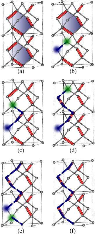
Figure 4: (Color online) Construction of the “string” defect (one magnetic flux) configuration from the maximally flippable R-state configuration (assuming periodic boundary conditions): (a) two adjacent 16-bond unit cells of the diamond lattice within the R-state, with flippable hexagons denoted by blue shading; (b) a pair of monomer excitations created by removing a dimer; (c), (d) and (e) monomers are separated. The dashed line shows the “string” of displaced dimers which connects them. (f) one of the monomers has traversed the cluster and the dimer is re-introduced. The resulting configuration has a single string excitation and a nonzero magnetic flux.

As discussed in Section II.2 and Section II.3 above, any given dimer configuration on the diamond lattice can be classified according to its total “magnetic” flux

$$\vec{\phi}=(\phi_{1},\phi_{2},\phi_{3})$$ (16)

where each component of $\vec{\phi}$ is a (topological) quantum number conserved under the dynamics of the quantum dimer model Eq. (1).

In a finite size cluster, each component of flux $\phi_{i}$ serves as a winding number which takes on an extensive number of (discrete) values. These are bounded by the size of the system, and can be expressed as combinations of the four occupation numbers $(n_{1},n_{2},n_{3},n_{4})$ which count the number of dimers on each of the four fcc sublattices of diamond-lattice bonds (equivalently, pyrochlore lattice sites). These occupation numbers are themselves invariant under the dynamics of the QDM. However the mapping between the occupation number representation (cf. Ref. bergman06-PRB, ), and the flux representation of these conserved quantities depends on the specific cluster geometry.

For the (100) cluster series we obtain the following expression:

$$\phi_{x} = \frac{1}{2L}(n_{1}-n_{2}-n_{3}+n_{4})$$

$$\phi_{y} = \frac{1}{2L}(n_{1}-n_{2}+n_{3}-n_{4})$$

$$\phi_{z} = \frac{1}{2L}(n_{1}+n_{2}-n_{3}-n_{4}),$$ (17)

where the corresponding positions of the sites in the 4-site elementary unit cell of the pyrochlore lattice are numbered

$$\mathbf{r}_{1} = (1,1,1)/4$$

$$\mathbf{r}_{2} = (-1,-1,1)/4$$

$$\mathbf{r}_{3} = (-1,1,-1)/4$$

$$\mathbf{r}_{4} = (1,-1,-1)/4$$

It follows that $-L^{2}/4\leq\phi_{i}\leq L^{2}/4$ for a cluster with $N=2L^{3}$ bonds in the diamond lattice (i.e. the number of sites in the pyrochlore lattice). In the highly symmetric ${\sf R}$–state (cf. Fig. 2) $n_{1}=n_{2}=n_{3}=n_{4}$. This state therefore belongs to the zero-flux sector $\vec{\phi}=(0,0,0)$.

In order to test the predictions of the effective field theory, notably Eq. (14), we need to be able to construct other states in neighbouring flux sectors. The flux quantum numbers $(\phi_{1},\phi_{2},\phi_{3})$ are conserved under all local operations which connect configurations satisfying the dimer constraint. However, we can construct states with finite magnetic flux, starting from the ${\sf R}$–state, by creating non-local “string” defects which traverse the periodic boundaries of the cluster.

We do this following the procedure illustrated in Fig. 4. When a dimer is removed from the lattice, two monomers (sites not touched by a dimer) are created. Subsequently, we can separate these monomers, creating a “string” of dimers which have been translated by exactly one bond. Moving a dimer by one bond reverses the sense of the magnetic field ${\mathbf{B}}$ associated with that dimer. We can therefore construct a state with a different flux by moving one of the monomers across the periodic boundary of the cluster in such a way that the two monomers meet and the dimer can be re-introduced. The resulting configuration fulfills again the zero-divergence condition on ${\mathbf{B}}$, but the magnetic flux through the periodic boundary traversed by the monomer has changed by exactly one unit. For a cubic cluster this is the smallest magnetic flux possible in the system, and we choose convention where $\phi=1$ in the new configuration. States with higher flux can be constructed by repeating the procedure above.

The monomers created by removing a dimer are excitations with fractional quantum numbers which depend on the original microscopic model, e.g. they might be fractional charges $e/2$ [fulde02, ], or “spinons” carrying spin $s=1/2$ [bergman06-PRL, ]. In field-theoretical terms, they are the magnetic monopoles of a $U(1)$ gauge theory, and the central question addressed in this paper is whether the QDM on a diamond lattice can support a quantum $U(1)$ liquid phase in which these monopoles are deconfined. In a finite size system, deconfined monopoles must be free to traverse the periodic boundaries of the cluster, and so the string defects described above also provide a direct test of monopole confinement — a necessary condition for monopole deconfinement in a periodic cluster is that the ground states in flux sectors connected by strings should be degenerate [c.f. Eq. (14)]. We return to this idea below.

II.5 Competing ordered phase

Figure 5: (Color online) Numbering convention in the definition of the order parameter $m_{\sf R}$ for the R-state (Eq. 18): (left) cubic cell of pyrochlore lattice with 16 sites, (right) corresponding diamond lattice cell with 16 bonds.

Table 2: Coefficients of bond occupation numbers within the six-dimensional irreducible representation used to define an order parameter for the ordered R-state, following Eq. (18).

	1	2	3	4	5	6	7	8	9	10	11	12	13	14	15	16
$f_{1}$	1	-1	-1	1	-1	1	1	-1	-1	1	1	-1	1	-1	-1	1
$f_{2}$	1	1	-1	-1	-1	-1	1	1	1	1	-1	-1	-1	-1	1	1
$f_{3}$	1	-1	1	-1	1	-1	1	-1	-1	1	-1	1	-1	1	-1	1
$f_{4}$	1	-1	-1	1	-1	1	1	-1	1	-1	-1	1	-1	1	1	-1
$f_{5}$	1	1	-1	-1	1	1	-1	-1	-1	-1	1	1	-1	-1	1	1
$f_{6}$	1	-1	1	-1	-1	1	-1	1	-1	1	-1	1	1	-1	1	-1

In order to determine the phase diagram of the quantum dimer model on a diamond lattice (cf. Fig. 1), we need also to characterize the competing ordered “R-state” [Refs. bergman06-PRL, ; bergman06-PRB, ]. The R-state (illustrated in Fig. 2) occupies the 8-site (16-bond) cubic unit cell of the diamond lattice (16-site on the pyrochlore lattice), and is 8-fold degenerate. The R-state breaks the inversion symmetry of the diamond lattice, its 8-fold degeneracy is best thought of as $2\times 4$ states with opposite chirality. The $4$ states with equal chirality can be related to each other with rotations or translations. In terms of the gauge field, this 8-fold degeneracy can be thought of as a 4-fold choice of $111$ axis (for a given tetrahedron), and a two fold choice of chirality about that axis. However for purposes of simulation it is easier to keep track of an order parameter defined in terms of the occupation numbers for dimers on diamond lattice bonds.

We define this through a 6-dimensional irreducible representation of the diamond lattice point group as follows

$$m_{\sf R}=\sqrt{\sum_{\eta=1}^{6}m^{2}_{{\sf R},\eta}},$$ (18)

where

$$m_{{\sf R},\eta}=\sum_{\xi=1}^{16}f_{\eta}^{\xi}\,n_{\xi}.$$ (19)

Here $m_{{\sf R},\eta}$ measures the occupancy of diamond lattice bonds/pyrochlore lattice sites, numbered as in Fig. 5, weighted by the factors $f_{\eta}^{\xi}$ given in Table LABEL:table.

Naively, one might have expected the order parameter to have been given by the sum of projectors

$$\sum_{\zeta=1}^{8}\langle{\sf R}_{\zeta}|\psi\rangle^{2}$$

where $|{\sf R}_{\zeta}\rangle$ are the 8 possible ordered R-states ($\zeta=1,2,...,8$). However,

$$\sum_{\zeta=1}^{8}\langle{\sf R}_{\zeta}|\psi\rangle=\frac{N}{4}$$

measures the total number of dimers (equal to one quarter of the number of pyrochlore sites), and the only linearly independent combinations of $|{\sf R}_{\zeta}\rangle$ are those given in Table. LABEL:table.

III Evidence for a quantum $U(1)$-liquid phase

III.1 Comments on simulations

In this section of the paper, we calculate the ground state properties of the quantum dimer model Eq. (1) using the Green’s Function Monte Carlo (GFMC) trivedi90 ; calandra98 method. This method has previously been applied very successfully to QDM’s in two dimensions ralko05 ; ralko06 ; ralko07 . We benchmark our GFMC simulations against results from exact diagonalization for small clusters, against a perturbation theory about the RK point for $\mu\to 1$ and, in Appendix D, against expansions about a perfectly ordered R–state for $\mu<0$. We chose to use GFMC because it automatically conserves the flux quantum numbers which are central to our study of the QDM, and because it can provide numerically exact answers for the ground state ($T=0$) properties of reasonably large clusters.

GFMC works by calculating a set of running averages on a random walk through configuration space, using on Hamiltonian matrix elements to move from one configuration to another. For large clusters and/or complicated problems, this random walk must be guided using a trial wave function, previously optimized by a suitable variational calculation. In this sense GFMC can perhaps best be understood as a systematic way of improving upon a known variational wave function.

In Appendix C we discuss a range of different variational wave functions which can be used to explore the ground state of the QDM on a diamond lattice. The most useful guide function we have found to date is :

$$|\psi^{\sf Var}_{\alpha\beta\gamma}\rangle_{\phi,{\sf c}}=\exp[\alpha N_{\sf f}+\beta m_{\sf R}+\sum_{\langle ij\rangle}\gamma_{ij}\tau_{i}\tau_{j}]|\psi_{\text{RK}}\rangle_{\phi,{\sf c}}$$ (20)

Here $|\psi_{\text{RK}}\rangle_{\phi,{\sf c}}$ is the equally weighted superposition of all dimer configurations within the maximally-connected subsector with flux $\vec{\phi}=(\phi_{1},\phi_{2},\phi_{3})$, i.e. those which are connected to an R-state by string excitations and/or matrix elements of Eq. (1). The sum $ij$ runs over pairs of hexagonal plaquettes within the diamond lattice, and $\tau_{i}=0$,$1$ is an Ising-like variable which takes on the value $\tau_{i}=1$ when the hexagonal plaquette $i$ is “flippable”. $N_{\sf f}=\sum_{i}\tau_{i}$ counts the total number of flippable plaquettes and $m_{\sf R}$ is the order parameter associated with the R–state, as defined in Eq. (18). The variational parameters $\alpha$, $\beta$ and $\gamma_{ij}$ are minimized using a stochastic reconfiguration algorithm sorella01 . For large lattices there are a many different pairs of hexagonal plaquettes. In practice we restrict ourselves to a set of up to 40 inequivalent $\gamma_{ij}$.

Our GFMC algorithm follows the prescription of [calandra98, ]. Simulations are typically performed using up to a few thousands of “walkers” in parallel. The transition probabilities between dimer configurations are calculated using the matrix elements from Eq. (1). If the guide wave function is exact (for example at the RK point, with all variational parameters set to zero) GFMC converges to the exact answer in a single step. Away from the RK point simulations typically converge after a few hundreds of reconfiguration steps. A “forward walker” technique is used to calculate the average value of the order parameter $m_{\sf R}$ [calandra98, ].

For $\vec{\phi}=0$, all simulations are started from a perfectly ordered R-state, and explore only dimer configurations connected with this. For more general $\vec{\phi}$, starting configurations are constructed using the prescription described in Section II.4. In neither case is the GFMC technique ergodic, in the sense of exploring all dimer configurations which might, in principle, contribute to the ground state. However GFMC performed in this way does produce results which are representative of the entire configuration space. This question is discussed at length in Section IV.

III.2 Death of an ordered state

We begin by studying how the ordered R-state evolves as a function of $\mu$. In Fig. 6 we present both VMC and GFMC simulation results for the order parameter $m_{\sf R}$, for $-0.2\leq\mu\leq 1$, in a series of cubic clusters of the form [100] which have the full symmetry of diamond lattice and have $2L^{3}$ bonds [cf. Table LABEL:table_g]. The linear dimension of the clusters ranges from $L=4$ (128 bonds) to $L=10$ (2000 bonds).

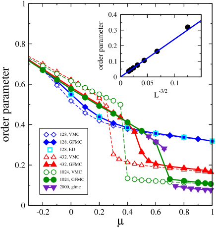
Figure 6: (Color online) Collapse of the ordered state: the order parameter $m_{\sf R}$ in the sector connected to the R-state. The results of VMC (dashed lines) and GFMC (solid lines) simulations are shown for series of clusters with cubic symmetry, and compared to exact diagonalization results for the smallest, 128 bond cluster. The inset shows finite size scaling of the order parameter at the RK point.

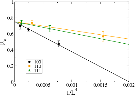
Figure 7: (Color online) Estimation of the critical value of $\mu_{c}(\infty)$ for the transition from the ordered R-state to the quantum $U(1)$-liquid, taken from GFMC simulation of three different families of clusters. Linear fits to $\mu_{c}(L)$ as a function of $1/L^{4}$ are made subject to the constraint that all data sets must converge to the same value $\mu_{c}(\infty)$ for $1/L\to 0$, regardless of the cluster geometry. We find $\mu_{c}(\infty)=0.75\pm 0.02$.

For the smallest 128-bond cluster we find very close agreement between GFMC and VMC simulations, and perfect numerical agreement between GFMC results and exact diagonalization calculations. This cluster is too small to be representative, but a point of inflection in $m_{\sf R}$ for $\mu\approx 0$ hints at a possible phase transition out of the R-state. For larger clusters, a first-order phase transition out of the R-state is clearly visible as a jump in the order parameter $m_{\sf R}$ at a critical value of $\mu=\mu_{c}(L)$. This jump is most pronounced in VMC calculations, where it occurs for smaller values of $\mu$, i.e. deeper inside the ordered state. The jump in the $m_{\sf R}$ shifts steadily to larger values of $\mu$ as the size of the system is increased. For the $L=6$, 432-bond cluster, a jump in $m_{\sf R}$ is observed in VMC for $\mu_{c}\approx 0.25$, and in GFMC for $\mu_{c}\approx 0.45$. Meanwhile for the largest $L=10$, 2000-bond cluster, the GFMC simulations suggest that this transition takes place for $\mu_{c}\approx 0.7$.

For $\mu_{c}(L)<\mu<1$, $m_{\sf R}(\mu)$ takes on a smaller, roughly constant value. However the finite size effects are large, with the value of $m_{\sf R}$ decreasing as the system size is increased. Much larger systems can be simulated at the RK point $\mu\equiv 1$, where the form of the ground state wave function is known exactly. Various methods of simulating at the RK point are discussed in Section IV. In the inset to Fig. 6, we show results obtained using local updates within the configurations explored by GFMC simulations. We find that $m_{\sf R}$ vanishes in the thermodynamic limit as $m_{\sf R}(\mu\equiv 1)\sim L^{-3/2}$.

Given the strong finite size effects visible in these data, it is important to make an estimate of $\mu_{c}(L\to\infty)$, to ensure that the competing phase for $\mu>\mu_{c}(L)$ does not collapse to a single point in the thermodynamic limit. The properties of the system for $L\to\infty$ must be independent of the cluster geometry, and so $\mu_{c}(L)$ should interpolate to the same value of $\mu_{c}(\infty)$ for all different families of clusters. In Fig. 7 we plot $\mu_{c}(L)$ as a function of $1/L^{4}$ for clusters of the type [100], [110] and [111], as defined in Table LABEL:table_g. All data collapse to a single value $\mu_{c}(\infty)=0.75\pm 0.02$. We note that the slightly different method of estimation used in Ref. sikora09, (fitting a separate line to each family of clusters) gave a very similar result $\mu_{c}(\infty)=0.77\pm 0.02$.

The fact that $\mu_{c}(\infty)-\mu_{c}(L)\sim 1/L^{4}$ provides strong, albeit indirect, evidence for the existence of the gapless photon excitations which are a signal feature of the quantum $U(1)$-liquid state. We can argue as follows : since the jump in $m_{\sf R}$ implies a first-order, zero-temperature phase transition, the finite size correction to $\mu_{c}$ must follow from the finite size corrections to the ground state energy of the two competing phases. All excitations about the R-state are gapped, and finite size corrections to its ground state energy should therefore be small. Assuming that the competing phase is a quantum $U(1)$-liquid with gapless photon excitations, the finite size corrections to its ground state energy will scale as $\sim 1/L^{4}$, as described by Eq. (15). Provided that the ground state energies of both states evolve smoothly near $\mu_{c}(L)$ (which is known to be true from both exact diagonalization and quantum Monte Carlo studies), finite size corrections to $\mu_{c}$ should also then scale as $\sim 1/L^{4}$.

On the strength of the simulation results for $m_{\sf R}$ presented above, it seems very reasonable to conclude that the phase diagram proposed in Fig. 1 is correct, with a single first-order phase transition from an ordered R-state to a quantum $U(1)$-liquid occurring for $\mu_{c}=0.75\pm 0.02$. In what follows, we present a variety of other evidence that this is indeed the case.

III.3 Collapse of monopole string tension

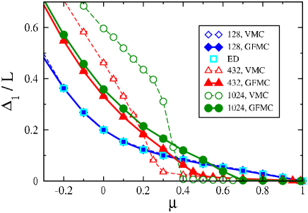
Figure 8: (Color online) Monopole string tension $\kappa_{1}$ [Eq. 21] for a range of $\mu$ spanning the ordered R-state and proposed quantum $U(1)$-liquid phase. Results are taken from VMC (dashed lines) and GFMC (solid lines) simulations for a series of clusters with cubic symmetry, and compared to exact diagonalization results for the smallest, 128 bond cluster.

If the state occurring for $\mu_{c}(L)<\mu<1$ is indeed a quantum $U(1)$-liquid, it should possess gapped, deconfined monopole excitations moessner03 . We can study the motion of these monopoles indirectly through the thought experiment used to construct configurations in different flux sectors in Section II.4. As illustrated in Fig. 4, separating the two monomers (monopoles) created by removing a dimer, destroys flippable hexagons along the “string” of dimers connecting the monomers. In the crystalline state, where the potential energy dominates, one can expect that there is a finite energy cost of such an operation, proportional to the length of the string. Where the string defect threads a periodic boundary of the cluster, its energy cost can be calculated as the gap to the ground state with one additional unit of flux.

We therefore define the “string tension” as the energy difference between the ground state in the zero-flux sector ($E_{0}$) and a sector with a single string defect ($E_{1}$), divided by the length of the string ($L$)

$$\kappa_{1}=\frac{E_{1}-E_{0}}{L}=\frac{\Delta_{1}}{L}$$ (21)

For the string defects considered, $L$ is simply the linear dimension of the cluster. This string tension is an indirect measure of the attractive, confining force between monopole excitations. It must therefore vanish in the deconfined quantum $U(1)$-liquid, but will be finite in the any ordered state.

In Fig. 8 we plot simulation result for the monopole string tension $\kappa_{1}$ as a function of $\mu$ for the same set of clusters and range of parameters as Fig. 6. Deep inside the ordered state, for negative values of $\mu$, classical effects dominate. A single string defect in a perfectly ordered R-state destroys $2L$ flippable hexagons at a potential energy cost of $2L|\mu|$. This linear relationship between $\kappa_{1}$ and $|\mu|$ for $\mu\lesssim 0$ is clearly visible in GFMC simulation results for the larger clusters. However the string tension drops rapidly as we approach the transition from the R-state into the competing phase at $\mu=\mu_{c}(L)$, and for large clusters it is essentially zero for $\mu_{c}(L)<\mu\leq 1$.

The coincidence between the jump in the order parameter $m_{\sf R}$ [Fig. 6] and the collapse in the string tension $\kappa_{1}$ [Fig. 8] lends yet more support to the proposed form of the phase diagram for the QDM on a diamond lattice [Fig. 1]. In particular, the absence of a string tension for $\mu_{c}(L)<\mu<1$ rules out the possibility that the competing phase is a different ordered state, for example a three-dimensional analogue of the resonating plaquette phase found in quantum dimer and quantum ice models in two dimensions rokhsar88 ; ralko08 ; shannon04 . However we still need to rule out the possibility that the competing phase is a different form of quantum liquid, by confirming explicitly that it is indeed the quantum $U(1)$-liquid we have been seeking. This is accomplished below.

III.4 Birth of a $U(1)$-liquid

Figure 9: (Color online) Reduction in the average number of flippable plaquettes $\Delta N_{\phi}$, as calculated in simulations at the RK point. (a) $-\Delta N_{\phi}$ plotted as a function of $\phi^{2}$ for cubic clusters of linear dimension $L=4$ (432 bonds) to $L=16$ (8192 bonds). (b) The same data set plotted as $-\Delta N_{\phi}/\phi^{2}$ vs $\phi^{2}$ to extract the leading dependence on $\phi$. (c) Finite-size scaling of the the coefficient of $\phi^{2}$ found from fits to $-\Delta N_{\phi}$ for clusters of linear dimension $L$ [cf. intercept to ordinate axis in (b), above]. The linear collapse of the coefficient of $\phi^{2}$ with $1/L$ is consistent with the prediction of the effective field theory for a quantum $U(1)$ liquid Eq. (14).

Figure 10: (Color online) Comparison of the energy gaps $\Delta_{\phi}$ found in GFMC simulations with the predictions of a perturbation theory about the RK point [Eq. (22)], for a range of $\mu$ within the proposed quantum $U(1)$-liquid phase. (a) Energy gap $\Delta_{\phi}$ normalized to $-\delta\mu=\mu-1$, to extract the leading dependence on $\mu$, and plotted as a function of $\phi^{2}$ [cf. Eq. (14)]. (b) Energy gap $\Delta_{\phi}$ normalized to $-\delta\mu\times\phi^{2}$, to extract the leading dependence on both $\mu$ and $\phi$, plotted as a function of $\phi^{2}$ [cf. Eq. (14)]. All results are for a 1024-bond cluster with cubic symmetry.

Within the field-theoretical scenario for a three dimensional QDM on a bipartite lattice, the quantum $U(1)$-liquid phase “grows” out of the RK point moessner03 ; bergman06-PRB . Exactly at the RK point, the ground states in all flux sectors are degenerate. Away from the RK point, in a finite size system, the ground state in the zero-flux sector has the lowest energy, and the (finite-size) energy gaps to the other low-lying flux sectors scale as $\Delta_{\phi}\sim c^{2}\phi^{2}/L$ [cf. Eq. (14)]. By construction, $c$ vanishes at the RK point.

Since the exact ground state is known at the RK point, we can calculate the finite size gaps $\Delta_{\phi}$ (and implicitly the speed of light $c$) within perturbation theory about the RK point. Writing

$${\mathcal{H}}_{\sf QDM}={\mathcal{H}}_{\sf RK}-\delta\mu\,\mathcal{N}_{\sf f}$$ (22)

where ${\mathcal{H}}_{\sf RK}$ is defined by Eq. (5), $\delta\mu=1-\mu$, and the operator $\mathcal{N}_{\sf f}$ is defined by Eq. (3), we find

$$\Delta_{\phi,{\sf MC}}=\Delta N_{\phi,{\sf MC}}\delta\mu+{\mathcal{O}}(\delta\mu^{2})$$ (23)

where

$$\Delta N_{\phi,{\sf MC}}=\langle{\mathcal{N}}_{\sf f}\rangle^{\sf RK}_{\phi,{\sf MC}}-\langle{\mathcal{N}}_{\sf f}\rangle^{\sf RK}_{0,{\sf MC}}$$ (24)

is the difference in the average number of flippable plaquettes between the zero-flux sector and the sector with flux $\phi$, calculated at the RK point, within the maximally-connected subsector of the Hilbert space, $\lambda_{c}={\sf MC}$. The maximally flippable R-state belongs to the zero-flux sector, and we therefore anticipate that $\Delta N_{\phi}<0$. If, as supposed, a quantum $U(1)$-liquid grows adiabatically from the RK point, then we must find

$$\Delta N_{\phi}\sim-\frac{\phi^{2}}{L}$$ (25)

In Fig. 9 we show results for $\Delta N_{\phi}$ obtained from simulation of a series of [100] cubic clusters with linear dimension ranging from $L=6$ (432 bonds) to $L=16$ (8192 bonds), for flux $\vec{\phi}=(\phi,0,0)$, plotted as a function of $\phi^{2}$. Simulations were performed within the maximally-connected subsector of states connected to the R-state for $\phi=0$, and within the subsector associated with a given number of string defects for higher values of flux. Due to large finite size effects, the expected linear relationship between $-\Delta N_{\phi}$ and $\phi^{2}$ is only visible for clusters with more than 2000 bonds. However the coefficient of $\phi^{2}$ can be extracted from a polynomial fit to $\Delta N_{\phi}$ as a function of $\phi$, at given $L$. This is found to be proportional to $1/L$, as shown in the inset to Fig. 9. From these results we obtain

$$c^{2}\approx 0.6\times\delta\mu$$ (26)

(in the present units) confirming that an incipient quantum $U(1)$-liquid is present at the RK point. This result is specific to the QDM on a diamond lattice. We note that simulations of the QDM on a cubic lattice yield quite different results olga-unpub .

In Fig. 10 we compare the results of the perturbation theory Eq. (23) with GFMC calculations made for a set of parameters bordering on the RK point, for a cluster of 1024 diamond lattice bonds. The energy gaps obtained from GFMC are plotted as $\Delta_{\phi}/(1-\mu)$ so to compare with perturbation theory, and as a function of $\phi^{2}$ so as to extract the leading behaviour of the $U(1)$-liquid phase. Both sets of data are found to show the same $\phi^{2}$ dependence on flux sector, confirming the existence of a quantum $U(1)$-liquid bordering the RK point.

III.5 A phase transition in a spectrum

Figure 11: (Color online) First order quantum phase transition from the ordered R-state into the quantum $U(1)$-liquid, as imaged in the finite size spectrum of a 1024-bond cluster. GFMC simulation results for the energy gap $\Delta_{\phi}$ are plotted as $\Delta_{\phi}/[\phi^{2}(1-\mu)]$ so as to collapse the spectra for the $U(1)$-liquid phase. The phase transition is visible as an abrupt qualitative change in the form of the spectra for $\mu=0.7$. The results of perturbation theory about the RK point (black line and points) are shown for comparison.

We are now in a position to draw a set of strong conclusions about the zero-temperature phase diagram of the QDM on a diamond lattice (cf. Fig. 1). For

$$\mu<\mu_{c}=0.75\pm 0.02$$

the ground state of the model is an ordered R-state. For $\mu_{c}<\mu<1$ it is a quantum $U(1)$-liquid with linearly dispersing photon excitations and deconfined magnetic monopoles. The quantum phase transition between these two phases at $\mu=\mu_{c}$ is first order. For $\mu\to 1_{-}$, the quantum $U(1)$-liquid is adiabatically connected with the RK point.

In Fig. 11 we present the results of GFMC simulations of a cubic 1024-bond cluster, for a range of parameters $0\leq\mu\leq 1$ spanning both the R-state and the quantum $U(1)$-liquid. We plot the energy gaps $\Delta_{\phi}$, rescaled as $\Delta_{\phi}/[\phi^{2}(1-\mu)]$ so as to collapse all data within the $U(1)$-liquid phase. Deep within the ordered phase the $\Delta_{\phi}$ should be proportional to both the linear dimension of the cluster and the flux (number of string defects), i.e.

$$\Delta_{\phi}^{\sf R}\sim L\times\phi$$

A plot of $\Delta_{\phi}/\phi^{2}$ at fixed $L$ should therefore show a clear distinction between a $U(1)$-liquid ($\Delta_{\phi}/\phi^{2}\sim\text{const.}$), and an ordered phase ($\Delta_{\phi}/\phi^{2}\sim 1/\phi$). For this cluster size a clear division is observed between $\mu\geq 0.7$ (liquid) and $\mu\leq 0.6$ (ordered). This is unambiguous evidence of a phase transition from a linearly confining phase to a quantum $U(1)$-liquid, imaged in a spectrum. The abrupt, qualitative change in the spectra for $\mu=0.6$ confirms that this phase transition is first-order in character.

IV Ergodicity and conservation laws within a given flux sector

IV.1 Lessons from exact diagonalization

Since GFMC uses on matrix elements of the QDM Hamiltonian [Eq. (1)] to connect different dimer configurations, it is guaranteed to respect the flux quantum numbers defined in Section II.4. However, not all dimer configurations with the same magnetic flux are connected by matrix elements of the Hamiltonian. Clearly, therefore, GFMC simulations for a given flux are not ergodic, in the sense that they do not explore all dimer configurations which might, in principle, contribute to the ground state for that flux sector. It is therefore very important to consider how the Hilbert space for a given flux $\vec{\phi}$ breaks up into different subsectors, and to ensure that simulations are carried out in the appropriate sub-sector(s). To this end, much can be learnt from the exact diagonalization of small clusters.

Figure 12: (Color online) (a) Block-structure of the Hamiltonian for the quantum dimer model on a diamond lattice, for an 128-bond cluster with a fixed value of the flux $\vec{\phi}=(0,0,0)$, following Table 3. Connected dimer configurations break up into different sub-ensembles. These can be divided into two groups, according to whether their transition graphs contain an odd or even number of loops. Both even and odd subsectors contain isolated configurations which do not participate in the dynamics of the model, and do not contribute to the ground state for $\mu<1$. (b) Contrasting block-structure of the Hamiltonian for the quantum dimer model on a square lattice for a finite size cluster with a fixed value of the flux $\vec{\phi}=(0,0)$. All dimer configurations which contribute to the ground state for $\mu<1$ belong to a single connected block. The remaining, isolated, dimer configurations do not participate in the dynamics of the model.

In total there are 115,150,848 dimer coverings of the $L=2$, 128-bond, cubic cluster. Of these, 11,835,352 have zero flux ($\phi=0$). These zero-flux configurations include 1440 isolated configurations with no flippable plaquettes, and 3072 configurations with a single flippable plaquette which connect only to a single other configuration. The remaining 11,830,840 configurations can be grouped into a small number of subsectors which are connected by the matrix elements of Eq. (1). These are listed in Table 3, and illustrated schematically in Fig. 12(a). This situation should be contrasted with the much simpler structure of the Hilbert space in the QDM on a square lattice, where all connected dimer configurations for a given value of flux $\vec{\phi}=(\phi_{x},\phi_{y})$ are associated with a single block of the Hamiltonian — cf. Fig. 12(b).

Table 3: Subsectors of the Hilbert space of the QDM on a diamond lattice with zero flux ($\phi=0$) for a cubic, 128-bond cluster. Subsectors are listed in order of increasing dimension, with isolated configurations and subsectors consisting of only two configurations omitted. The largest, maximally-connected, subsector (A) contains the R-states. Further subsectors can be obtained through cyclic permutations of dimers on closed loops — the 8-link loop operation shown in Fig. 13 provides access to subsector B. Subsectors can be classified according to the number and type of loops in their transition graph.

subsector label $\lambda_{c}$	multiplicity	dimension	number of loops in transition graph (mod 2)	longest irreducible loop in transition graph
A	1	7794744	0	2
B	1	3468032	1	8
C	3	131584	0	10
D	3	45184	0	14
E	8	3376	0	14
F	192	40	1	12

For this 128-bond cluster, about two-thirds of the configurations with $\phi=0$ belong to a maximally-connected subsector, labelled A in Table 3, which includes the R-states. The vast majority of the remaining configurations — about one-third of the total — are found in one other subsector, labelled B in Table 3. Subsector B can be accessed from the maximally connected subsector by acting on a randomly chosen configuration with the update shown in Fig. 13 — the cyclic permutation of dimers around a closed, 8-link loop. Interestingly, this 8-link permutation is the sub-leading term for dimer dynamics in the derivation of the QDM from Eq. (7) or Eq. (II.1).

Subsectors C, D, E and F cannot be accessed from subsector A using the 8-link loop alone. However they can be reached by cyclically permuting dimers within suitably chosen configurations belonging to subsector A, on loops of length 10, 14, 14 and 12, respectively. Since the number and length of possible such loops grows with the size of the system, we anticipate that the number of subsectors in the Hilbert space grows with system size. We put these observations on a more formal footing below.

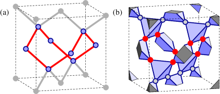
Figure 13: (Color online) 8-link “loop” used to connect dimer configurations within subsectors A and B of the Hilbert space of the QDM on a diamond lattice [cf. Table 3]. (a) 8-link loop of bonds within the cubic unit cell of the diamond lattice. Three distinct 8-link loops of this type are possible, each of which appears octagonal when projected into an appropriate [100] plane. Where exactly 4 bonds are occupied by dimers, this loop is “flippable”, i.e. a new state obeying the dimer constraint can be obtained by cyclicly permuting those dimers around the loop. (b) equivalent 8-link loop of sites within the cubic unit cell of the pyrochlore lattice.

IV.2 A hidden quantum number

The way in which the Hilbert space of the QDM on a diamond lattice breaks up into distinct blocks suggests the existence of further, conserved quantities besides magnetic flux $\phi$. We can gain more insight into this problem, and understand the action of the 8-link loop shown in Fig. (13) by studying transition graphs.

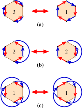
Figure 14: (Color online) Schematic representation of all possible changes in the topology of a transition graph which follow from the cyclic permutation of dimers on a hexagonal 6-link loop. Red lines denote loop segment with a single dimer. Blue lines denote a loop segment with an odd number dimers. All loop segments, whether red or blue, start and finish on sites belonging to different sublatticies of the (bipartite) diamond lattice, denoted here by filled or empty circles. The number of loops associated with each section of the transition graph is shown in the middle of the hexagonal plaquette. This number changes by either 0 or 2.

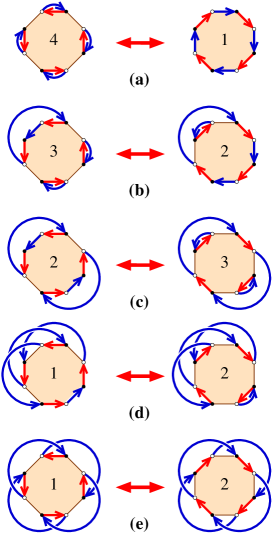
Figure 15: (Color online) Schematic representation of all possible changes in the topology of a transition graph which follow from the cyclic permutation of dimers on an 8-link loop. The number of loops of the transition graphs changes by either 1 or 3.

A transition graph is the set of directed loops formed by overlaying two dimer configurations on a bipartite lattice, and drawing arrows from A to B sublattice on those bonds which are occupied by a dimer in the first configuration, and from B to A sublattice on those bonds which are occupied by dimers in the second configuration rokhsar88 . Cyclicly permuting the dimers on the loops of the transition graph converts the first configuration into the second (and vice versa). By construction, these loops cannot intersect one another — although one loop may be threaded through another in a three-dimensional lattice.

A pair of dimer configurations are connected if (and only if) we can undo all the long loops in their transition graph using only matrix elements of Eq. (1) — cyclic permutations of dimers on a 6-link hexagonal plaquette — so that only trivial “loops” occupying a single bond remain. These trivial loops have length 2, and the maximum number of trivial loops achievable is equal to the number of dimers in the system — an even number for all of the clusters considered in this paper. In Fig. 14 we enumerate the three possible, topologically distinct, changes in the transition graph associated with the cyclic permutation of dimers on an hexagonal plaquette. In each case the total number of loops in the transition graph changes by an even number — either 0 or 2.

Cyclic permutations of dimers on an 8-link loop have a somewhat richer structure, illustrated in Fig. 15. In this case, the total number of loops in the transition graph changes by an odd number — either 1 or 3. Consequently, the action of 8-link loop cannot be undone using matrix elements of the Hamiltonian [Eq. (1)] alone.

More formally, we can associate a unique transition graph with each distinct dimer configuration by choosing one particular dimer configuration as reference (for present purposes, an R-state is a convenient choice). The number of loops in this transition graph, modulo 2, is then a conserved quantity within the dynamics of the QDM Eq. (1). Furthermore, it must be even in the subsector connected with the R-state. In Table 3 we classify the all of the different subsectors of the zero-flux sector of the 128-bond cubic cluster containing more than two configurations according to this new, Ising, quantum number.

Examination of transition graphs also provides some insight into the other, smaller, subsectors of the Hilbert space, labelled C, D, E and F in Table 3. Empirically, we find that these can be accessed from the maximally-connected subsector containing the R-states (subsector A) through the cyclic permutation of dimers on suitably chosen loops of length 10, 12, and 14. Closed loops in the transition graph can generally be contracted through the repeated permutation of dimers on 6-link loops of the type found in the Hamiltonian Eq. (1). By construction, all non-trivial loops in the transition graph for two configurations within subsector A can be removed in this way, leaving only trivial loops of length 2. The different subsectors B—F listed in Table 3 can therefore be classified according to the longest irreducible loop in their transition graph with a (suitably chosen) state within subsector A. The lengths of the irreducible loops are listed in Table 3.

It is interesting to note that the Ising quantum number associated with the number of loops in the transition graph is even where the longest irreducible loop is of length 2, 10 or 14, and odd where the longest irreducible loop is of length 8 or 12. We infer (but have not proved) that topological selection rules of the form illustrated in Fig. 14 apply for updates based on loops of length 6, 10, 14…, and of the form illustrated in Fig. 15 for updates based on loops of length 8, 12, 16…Cyclic permutations on loops of length 6, 10, 14…are precisely the form of dynamics permitted for (spinless) fermionic models of the form Eq. (7), while bosonic models also permit cyclic permutations on loops of length 8, 12, 16….schwandt10 We therefore speculate that the number of loops in the transition graph will be a conserved quantity (mod 2) for the most general QDM Hamiltonian derived from a fermionic model on a pyrochlore lattice, but not for the equivalent bosonic or spin model.

Clearly, more questions could be asked about the non-ergodicty of the QDM on a diamond lattice. What, for example, are the the conserved quantities which distinguish the smaller subsectors of the Hilbert space ? And how do the number, multiplicity, and dimension of these subsectors grow with the size of the system ? For the purposes of this paper, however, the most pressing need is to understand the impact of this non-ergodicity on the simulations described in Section III. It is this to which we now turn.

IV.3 Can we trust simulations ?

It is clear from the analysis above that QDM on a diamond lattice is not ergodic within a given flux sector. The analysis which leads to the phase diagram Fig 1 rests on simulations performed within the (maximally connected) subsector of states connected to the R-state by the matrix elements of Eq. (1), and on the systematic construction of configurations with finite flux using “string” defects’ [cf. Fig. (4)]. Before we can have full confidence in these results we must therefore address the following question :

What bias do we introduce into our results by simulating only within these subsectors of the Hilbert space ?

The enumeration of states for an 128-bond cluster confirms the common-sense expectation that we can access the largest subsector of the Hilbert space for zero flux by seeding simulations from an R-state. Moreover, we now understand how to extend these simulations to configurations with an odd number of loops in their transition graph, through use of an 8-link loop. However there remain a non-vanishing fraction of dimer configurations — about 5% for the 128-bond cubic cluster [Table 3] — which can only be reached by other, more complex updates.

It seems reasonable to expect that these unsociable configurations will (a) contribute little to the ground state wave function and (b) constitute a vanishing fraction of the total number of dimer configurations in the thermodynamic limit. However this reasonable expectation must be approached with some caution, not least because, in the absence of a full understanding of conserved quantities, it is hard to assess how these neglected corners of the Hilbert space grow with system size.

We can most easily get a handle on the consequences of non-ergodicity at the RK point, where simulations for ground state properties amount to performing classical averages over all dimer configurations within a given flux sector. These can be performed in several different ways

1. As in Section III.4, using “local” updates based on the matrix elements of the Hamiltonian.

2. Using a “loop” algorithm developed for the simulation of ice models newman07 ; hermele04 .

3. Using a “worm” algorithm based on movement of monomers barkema98 .

In the “loop” algorithm, a directed random walk along bonds is used to construct a self-intersecting path in which all flux arrows associated with dimers have the same sense. The dimers which lie along this path are each cycled one link further along, reversing the sense of the flux around the closed “loop”, while preserving the dimer constraint.

In the “worm” algorithm, a single dimer is removed, and the two monopoles created are allowed to diffuse freely around the lattice until they meet, at which point the missing dimer is re-introduced. We have checked explicitly that “loop” and “worm” simulations lead to identical results for the QDM on the diamond lattice, and concentrate here on comparing results obtained using “local” and “loop” updates.

A necessary condition for the existence of a quantum $U(1)$-liquid in a QDM is that the average number of flippable plaquettes in the dimer configurations belonging to a given flux sector scale as $\Delta N_{\phi}=N_{\sf f}(\vec{\phi})-N_{\sf f}(\vec{0})\sim-\phi^{2}/L$ [Eq. (25)]. In Fig. 16(a) we compare the probability distribution for the number of flippable plaquettes $N_{\sf f}$ calculated for all dimer configurations within the zero-flux sector (green, shaded columns) with that calculated within the maximally connected subsector containing the R-state (columns without shading). Identical results were obtained both within simulation, using “loop” updates to explore all dimer configurations, and “local” updates to access to the maximally-connected subsector, and within exact diagonalization, by explicit enumeration of all dimer configurations. The probability distribution for the number of flippable plaquettes is markedly different in the two cases, and the mean value of $N_{\sf f}$ clearly higher for the subset of configurations connected with the R-state.

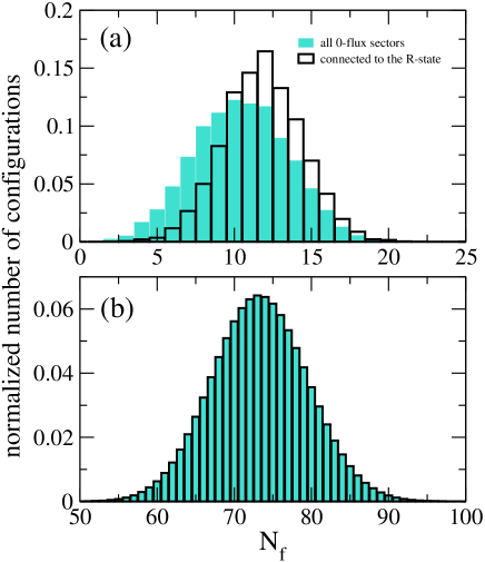
Figure 16: (Color online) Histogram of the number of flippable plaquettes in different sets of dimer configurations, calculated at RK point. (a) Results for an 128-bond cubic cluster, calculated within in the entire zero-flux sector (blue, shaded columns), and in the subsector connected to the R-state (unshaded columns). (b) Equivalent results a for an 1024-bond cluster.

At first sight this disagreement might seem rather alarming, but it is simply a finite-size effect. In Fig. 16(b) we present the results of an identical study for a larger, 1024-bond cluster. The same, Gaussian, probability distribution with mean $\langle N_{\sf f}\rangle=73.27$ and variance $\sigma_{N_{\sf f}}=6.21$ is found for both the full set of dimer configurations sampled by the “loop” algorithm, and the maximally-connected subsector explored by the “local” updates. Similar gaussian probability distributions are found in sectors of the Hilbert space with finite flux, and are again independent of the method of simulation.

There are two obvious possible explanations as to why the same probability distribution should be found for averages calculated at the RK point in the full set of dimer configurations, and those calculated within its maximally-connected subsector. One is that the relative size of the maximally-connected subsector grows with system size, so that it comes to dominate all averages in the thermodynamic limit. The other is that all large blocks of the Hilbert space (within a given flux sector) are statistically very similar. This might occur if, for example, configurations in different subsectors differed only by some local defect which could not be removed using matrix elements of the Hamiltonian, but which had no impact on the bulk properties of the state.

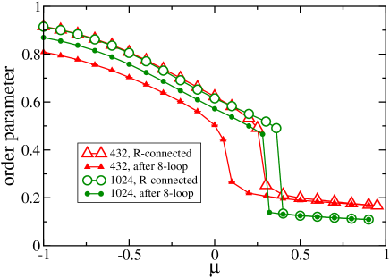
Figure 17: (Color online) $\mu$-dependence of the order parameter $m_{\sf R}$ for the R-state, within two different subsectors of the Hilbert space: starting from the R-state in flux $\phi=0$ subsector (open symbols) and in the subsector that is connected to it by an 8–site loop (solid symbols). Results are calculated using Variational Monte Carlo simulation for cubic clusters with 432 (triangles) and 1024 (circles) diamond-lattice bonds.

To distinguish between these alternatives we can examine how quantum Monte Carlo simulation results in the two largest subsectors of the Hilbert space depend on the subsector ${\lambda_{c}}$ in which they are carried out. In Fig. 17 we present the results of a Variational Monte Carlo study of the order parameter $\langle m_{\sf R}\rangle_{\lambda_{c}}$, for a cubic 432 and 1024-bond clusters. Simulations were carried out within

1. the subsector with flux $\phi=0$ containing the R-state;

2. the subsector with flux $\phi=0$ obtained by acting with an 8-link loop update on a randomly chosen state from the subsector containing the R-state.

Within the crystalline, ordered phase, an 8–loop update reduces the $m_{\sf R}$ relative to the subsector containing the R-state. This reduction in order parameter scales as $1/L^{3}$ — as would be expected for a local defect into an ordered state — and vanishes in the thermodynamic limit. Meanwhile the energy cost of the 8–loop update is a constant in the ordered state. This behaviour should be compared with the topological string defect used to change flux sector acting in the R-state ordered phase, whose effect on the order parameter scales as $1/L^{2}$, and which creates a finite size energy gap $\propto L$.

In marked contrast, the simulation results for $\langle m_{\sf R}(\mu)\rangle$, in the quantum $U(1)$-liquid phase are independent of the subsector within which they are calculated. Intuitively, we imagine that as the R-state order melts into the $U(1)$-liquid phase, so defects in the order parameter melt, too, leaving only an invisible partition in the Hilbert space.

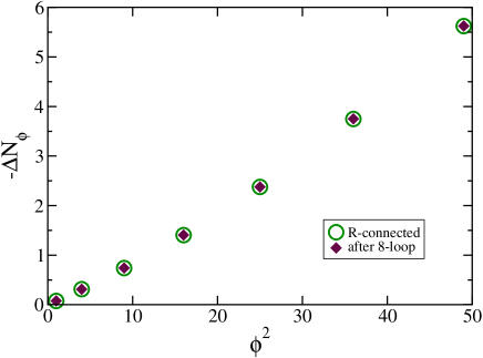
Figure 18: (Color online) The difference in the average number of flippable plaquettes $\Delta N_{\phi}$ [Eq. (24)], calculated at the RK point for dimer configurations in different subsectors of the Hilbert space. Green circles denote results for configurations connected to the R-state by matrix elements of Eq. (1) and string defects. Maroon diamonds denote results for configurations containing an additional 8-link “loop” defect. All results are for a cubic 1024-bond cluster.

We have repeated this analysis for more general local defects in the R-state, seeding simulations from configurations generated using randomly chosen loops with 10, 12, 14, 16, 18 and 20 links, applied states within the subsector containing the R-state. After simulation starting from a configuration obtained using one 10-, 14- or 18-link loop we recover the same values of $\langle m_{\sf R}(\mu)\rangle$ as in the maximally connected sector containing the R-state. Meanwhile simulates started from a configuration obtained using an 12-, 16- or 20-link loop exhibit the same values of $\langle m_{\sf R}(\mu)\rangle$ as those in the second large subsector accessed using the 8-link loop.

This is consistent with our analysis of the transition graphs: the 8-loop cannot be undone by Hamiltonian matrix updates and so we remain in a subsector not connected to R-state, for which the average value of the order parameter has to be lower. Loops of length 10, 14, 18… can typically be reduced to 6-link loops so that the resulting configuration remains in the maximally connected sector, while loops of length 12, 16, 20… can be reduced to an 8-link and 6-links loops, leading to the second large subsector. Although we do not have a precise understanding of the origin of the additional subsectors found in the 128-bond cluster [Table 3], from our simulation for larger systems we tentatively conclude that the statistically accessible configurations with an even(odd) number of loops in their transition graph are of the type A and B (i.e. connected to the ${\sf R}$ state directly or by a single 8–link loop).

It is also interesting to compare the changes in the liquid phase ground state energy in detail. The ground state energy in all subsectors must be zero at the RK point. In the liquid phase bordering on the RK point, the gaps between states with different magnetic flux should scale as $\Delta_{\phi}\sim\phi^{2}/L$ [Eq. (14)]. This in turn implies that, at the RK point, $\Delta N_{\phi}\sim-\phi^{2}/L$ [Eq. (25)]. In Fig. 18 we present the results of simulations carried out in maximally-connected subsector for each $\phi$, and in the subsector connected to it by a single, local, 8-link “loop” defect. The differences in the values of $\Delta N_{\phi}$ obtained in the two subsectors are smaller than the error bars on the simulation.

This analysis represents only a partial solution to the problem of how to understand different subsectors within the Hilbert space of a three-dimensional QDM. However for the purposes of this paper, we gain confidence that GFMC simulations performed in the maximally-connected subsector, following the prescriptions of Section II and Section III, do give reliable estimates of the ground state properties of the QDM on a diamond lattice.

We can trust these estimates in the ordered, R-state, because the alternative subsectors correspond to excited states, and not to the ground state. And we can trust the estimates in the quantum $U(1)$-liquid phase because in that case all statistically significant subsectors contribute equally to the ground state. Thus, while the QDM on a diamond lattice is not ergodic within a given flux sector, this lack of ergodicity has no pathological consequences for the ground state phase diagram as we have calculated it. Our initial analysis suggests that the same may not be true of the QDM on a cubic lattice olga-unpub .

V Conclusions

In this paper we set out to show that a three-dimensional quantum dimer model (QDM) — the QDM on a bipartite diamond lattice — could support a quantum liquid ground state, whose excitations include linearly dispersing photons and deconfined magnetic monopoles of an underlying $U(1)$ gauge theory. We have identified the order parameter associated with the competing, ordered “R-state” and, through use of quantum Monte Carlo simulation, have shown that it is finite only where the ratio $\mu$ of kinetic to potential energy terms in the QDM Hamiltonian is less than $\mu_{c}=0.75\pm 0.02$. We have further shown that (a) the string-tension associated with separating a pair of monomers (magnetic monopoles) vanishes for $\mu>\mu_{c}$, and (b) the finite-size energy spectrum for $\mu_{c}<\mu\leq 1$ is consistent with the predictions of the Maxwell action of conventional quantum electromagnetism.

We conclude that the QDM on a diamond lattice undergoes a first-order phase transition from an ordered R-state into a quantum $U(1)$ liquid phase at $\mu=\mu_{c}$. This liquid phase occupies an extended region of parameter space, terminating at the RK point $\mu=1$. This completes the analysis outlined in our earlier Letter [Ref. sikora09, ], and confirms the validity of the phase diagram Fig. 1, previously proposed in Refs moessner03, ; bergman06-PRB, on the basis of field-theoretical arguments.

We have also explored how the Hilbert space of the QDM on a diamond lattice breaks up into different, disconnected, subsectors, and identified a new, Ising, quantum number associated with the number of loops in the transition graph of a given dimer configuration. We argue that the lack of ergodicity within any given flux sector does not have pathological consequences for the ground state phase diagram, as found by quantum Monte Carlo simulations. We further show that the same ground state phase diagram is obtained, regardless of whether the dimers are treated as bosonic or fermionic objects.

Taken together, these results would seem to set the existence of a quantum $U(1)$ liquid phase in the QDM on a diamond lattice beyond reasonable doubt. However the very fact that such a state exists in this model begs all manner of other questions. Do other quantum dimer models on bipartite lattices in three dimension — for example the cubic lattice — also support quantum $U(1)$ liquids, as conjectured in Ref. moessner03,  ? What are the nature and consequences of the additional quantum numbers associated with the non-ergodicity of three-dimensional quantum dimer models ? Which other models can support a quantum $U(1)$ ground state, and for what range of parameters ? An obvious candidate in this case is the quantum loop model studied in Ref. hermele04, . Here we find evidence for a quantum $U(1)$ liquid for $-0.5<\mu<1$, which will be presented elsewhere shannon-arXiv .

The greatest excitement, however, would attend to finding a quantum $U(1)$ liquid phase in experiment, and identifying its deconfined, fractional excitations. Here more quantitative analysis is needed, both to pin down the characteristics of these excitations, and to bridge the gap between idealized models such as Eq. (1), and real materials or artificial assemblies of cold atoms. Since the coherence temperature of the quantum $U(1)$ liquid will be low in either case, both finite temperature effects banerjee08 , and the consequences of competing interactions, need to be explored in more detail.

VI Acknowledgements

It is our pleasure to acknowledge helpful conversations with Kedar Damle, Yong-Baek Kim, Andreas Läuchli, Gregoire Misguich, Roderich Moessner, and Arno Ralko. We are particularly indebted to Federico Becca for advice and encouragement with simulation techniques. This work was supported under EPSRC grants EP/C539974/1 and EP/G031460/1, Hungarian OTKA grants K73455, U.S. National Science Foundation I2CAM International Materials Institute Award, Grant DMR-0645461, and the guest programs of MPI-PKS Dresden and YITP, Kyoto.

Appendix A Absence of a fermionic sign problem

All results for $H_{\text{QDM}}$ are obtained under the assumption that the dimers are bosonic objects, i.e., exchanging two dimers does not yield a phase. However, as we show in this Appendix, the same effective model can be used to describe the fermionic case.

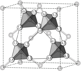
Figure 19: (Color online) Labeling of the sites of the pyrochlore lattice by enumerating one of the two types of tetrahedra and four sublattices on each tetrahedron. This labeling allows us to show that the Hamiltonian $H_{\text{QDM}}$ has no fermionic sign problem even if the underlying particles are fermions.

Let us now assume that the dimers are objects which are created (annihilated) by fermionic operators $c^{{\dagger}}_{i,\sigma}$ ($c^{\vphantom{{\dagger}}}_{i,\sigma}$). The index $i\in\{1,\dots,n\}$ refers to a tetrahedron and the index $\sigma\in\{1,2,3,4\}$ refers to the site on that tetrahedron (see Fig. 19). Since the diagonal part $\mathcal{N}_{f}$ of the Hamiltonian in $H_{\text{QDM}}$ is not affected by changing to fermions, we only focus on the ring-exchange processes. These can be written in terms of the fermionic operators as

$${\mathcal{K}}_{\sf f}=\sum_{\;\pspicture(0.0pt,2.84526pt)(5.69054pt,8.53581pt)\psset{linewidth=0.85358pt,linestyle=solid}{\psset{}\pspolygon(0.0pt,2.20508pt)(0.0pt,6.40186pt)(3.52814pt,8.53581pt)(7.25545pt,6.40186pt)(7.25545pt,2.20508pt)(3.52814pt,0.0pt)}\endpspicture\;}\left(c^{{\dagger}}_{i_{a},\sigma_{a}}c^{\vphantom{{\dagger}}}_{i_{a},\sigma_{a}^{\prime}}c^{{\dagger}}_{i_{b},\sigma_{b}}c^{\vphantom{{\dagger}}}_{i_{b},\sigma_{b}^{\prime}}c^{{\dagger}}_{i_{c},\sigma_{c}}c^{\vphantom{{\dagger}}}_{i_{c},\sigma_{c}^{\prime}}+H.c.\right),$$ (27)

where the sum is taken over all hexagons, and $i_{a}<i_{b}<i_{c}$. We thus choose only one of the twelve different ways of how the three fermions can hop around the hexagon.

We show now that all twelve ways, which are resulting from clockwise/counter-clockwise processes as well as different sequences, have a positive matrix element. (i) Fermion configurations which result from clockwise or counter-clockwise processes are related by an even number of fermion exchanges, e.g. $(1,2,3)\leftrightarrow(2,3,1)$, and thus have the same sign. In passing we mention that this is generally true for ring-hopping processes which involve an odd number of fermions, while processes with an even number of fermions have the opposite sign and thus cancel each other. (ii) the matrix-element does not depend on the sequence in which the fermions hop. This can be seen if we choose “ordered” fermion configurations with respect to the tetrahedra, i.e., we fill the vacuum $|0\rangle$ by

$$|c\rangle=c^{{\dagger}}_{i_{N},\sigma_{N}}\dots c^{{\dagger}}_{i_{2},\sigma_{2}}c^{{\dagger}}_{i_{1},\sigma_{1}}|0\rangle.$$ (28)

Because of the hardcore-dimer constraint, there is at most one fermion on each tetrahedron $i$ which then has an arbitrary $\sigma$. In Hamiltonian (27), the fermionic operators come in pairs for each $i$ and thus there is always an even number of fermionic operators which need to be exchanged to evaluate the matrix elements. Thus, the sign does not depend on the sequence in which the operator pairs are applied and all non-zero matrix elements are equal to $+1$. The argument works only for the dimer model. If we consider a related loop model on the same lattice, there are two fermions per tetrahedron (i.e., two dimers attached to each site) and the sign problem can no longer be avoided using this method.

Appendix B Landau theory for R-state

In this paper we studied the zero-temperature quantum phase transition from the ordered R-state into a quantum $U(1)$-liquid. However we note that the finite-temperature, phase transitions between ordered and classical $U(1)$ “Coulomb” phases in three-dimensional classical dimer models have also proved be a very interesting huse03 ; alet06 ; powell08 ; chen09 . These phase transitions do not fall into the conventional Landau paradigm, since the high temperature Coulomb phase exhibits the power-law decay of correlation functions characteristic of a $U(1)$ gauge theory, rather than the exponential decay predicted by a Ginzburg-Landau theory of the low-temperature ordered state.

In this context it is interesting to note that the present order parameter symmetry permits a third-order invariant in a Landau action, as well as the usual quadratic and quartic terms :

$$\Delta_{\sf R} = a\sum_{i=1}^{6}m_{{\sf R},i}^{2}$$

$$+b\left(m_{{\sf R},1}m_{{\sf R},2}m_{{\sf R},3}+m_{{\sf R},4}m_{{\sf R},5}m_{{\sf R},6}\right)$$

$$+c_{1}\sum_{i=1}^{6}m_{{\sf R},i}^{4}+c_{2}\left(\sum_{i=1}^{6}m_{{\sf R},i}^{2}\right)^{2}$$

$$+c_{3}\left[\left(m_{{\sf R},1}^{2}+m_{{\sf R},2}^{2}+m_{{\sf R},3}^{2}\right)^{2}\right.$$

$$+\left.\left(m_{{\sf R},4}^{2}+m_{{\sf R},5}^{2}+m_{{\sf R},6}^{2}\right)^{2}\right]$$

$$+c_{4}\left(m_{{\sf R},1}^{2}m_{{\sf R},4}^{2}+m_{{\sf R},2}^{2}m_{{\sf R},5}^{2}+m_{{\sf R},3}^{2}m_{{\sf R},6}^{2}\right)^{2}$$

In the ordered phase with $\langle m_{\sf R}\rangle=m\neq 0$, the cubic term selects eight possible configurations. For $b<0$ these have the form given in Table 4, and are of course the eight R-state configurations, which become exact ground states of the quantum problem in the limit $\mu\to-\infty$. For $b>0$ the cubic term does not select a valid (static) dimer configuration.

Table 4: Eight R-states selected by the cubic invariant $b<0$ in Eq. (LABEL:Eq:invariant), expressed in terms of the coefficients of the order parameter Eq. (18), within an ordered state with $m=\langle m_{\sf R}/\sqrt{3}\rangle$. The four R-states labelled $\zeta=1,\ldots,4$ have the opposite chirality from those labelled $\zeta=5,\ldots,8$.

$\zeta$	$m_{{\sf R},1}$	$m_{{\sf R},2}$	$m_{{\sf R},3}$	$m_{{\sf R},4}$	$m_{{\sf R},5}$	$m_{{\sf R},6}$
1	$m$	$m$	$m$	0	0	0
2	$m$	$m$	$-m$	0	0	0
3	$-m$	$m$	$-m$	0	0	0
4	$-m$	$-m$	$m$	0	0	0
5	0	0	0	$m$	$m$	$m$
6	0	0	0	$m$	$-m$	$-m$
7	0	0	0	$-m$	$m$	$-m$
8	0	0	0	$-m$	$-m$	$m$

Appendix C Comparison of variational wave functions

In this Appendix we explore the transition from solid to liquid phases of the quantum dimer model on a diamond lattice using a variety of variational wave functions. This is an essential preliminary to Green’s function Monte Carlo (GFMC) simulations, which rely on importance sampling of configurations to achieve convergence in a finite time. Except where stated otherwise, the calculations presented here were performed using variational Monte Carlo, within the stochastic reconfiguration algorithm sorella01 ; capello05 , for a 1024-bond cluster with cubic symmetry.

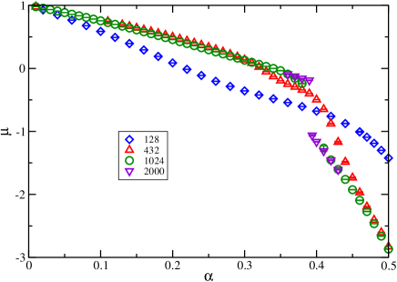
Figure 20: (Color online) Value of $\mu$ for which the one-parameter variational wave function $|\psi^{\sf Var}_{\alpha}\rangle$ [cf. Eq. (30)] has the lowest energy, as a function of the variational parameter $\alpha$. Results are plotted for cubic clusters ranging in size from 128 to 2000 bonds.

Perhaps the simplest wave function we can consider is

$$|\psi^{\sf Var}_{\alpha}\rangle_{\phi,{\sf c}}=\exp\left[\alpha{\mathcal{N}}_{\sf f}\right]|\psi_{\sf RK}\rangle_{\phi,{\sf c}}$$ (30)

where $\alpha$ is the single variational parameter associated with the total number of flippable hexagons ${\mathcal{N}}_{\sf f}$, and $|\psi_{\sf RK}\rangle_{\phi,{\sf c}}$ is the RK point ground state function, i.e. the equally weighted sum of all dimer configurations within a given subsector of the Hilbert space. In the discussion of ground state properties which follows, we will consider the maximally connected subsector for $\vec{\phi}=0$, which comprises all dimer configurations connected to an R-state by matrix elements of Eq. (1).

We can view Eq. (30), as the Jastrow form which follows from Eq. (22). For this reason we anticipate that this wave function will work well in the vicinity of the RK point, but will tend to over-emphasize any liquid phase occurring for $\mu\to 1$. The wave function $|\psi^{\sf Var}_{\alpha}\rangle_{\phi,{\sf c}}$ has the advantage that the value of $\mu$ which minimizes the ground state energy for a given $\alpha$ can be found by evaluating averages at the RK point

$$\mu=\frac{\frac{1}{2}\langle\mathcal{N}_{\sf f}\mathcal{K}_{\sf f}+\mathcal{K}_{\sf f}\mathcal{N}_{\sf f}\rangle_{\sf RK}-\langle\mathcal{K}_{\sf f}\rangle_{\sf RK}\langle\mathcal{N}_{\sf f}\rangle_{\sf RK}}{\langle\mathcal{N}_{\sf f}^{2}\rangle_{\sf RK}-\langle\mathcal{N}_{\sf f}\rangle_{\sf RK}^{2}}$$ (31)

where $\mathcal{K}_{\sf f}$ is defined by Eq. (2). In Fig. 20 we present results for $\mu$ as a function of $\alpha$ for cubic clusters ranging in size from 128 to 1024 diamond lattice bonds. It is tempting to interpret the abrupt change in $\partial\mu/\partial\alpha$ at $\alpha\approx 0.4$, $\mu\approx-0.5$ as evidence of a first order phase transition. However comparison with exact diagonalization, and with other variational wave functions below, suggests that $|\psi^{\sf Var}_{\alpha}\rangle$ gives very poor energies away from the RK point, and is only really useful for $\mu\to 1$.

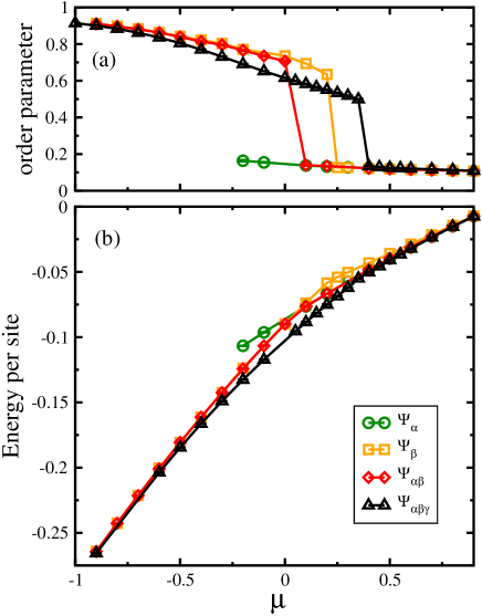
Figure 21: (Color online) Comparison of different variational wave functions for 1024-bond cluster: (a) order parameter and (b) energy per site: (green) $|\psi^{\sf Var}_{\alpha}\rangle$ [cf. Eq. (30)] (orange) $|\psi^{\sf Var}_{\beta}\rangle$ [cf. Eq. (32)]; (red) $|\psi^{\sf Var}_{\alpha\beta}\rangle$[cf. Eq. (33]); (black) $|\psi^{\sf Var}_{\alpha\beta\gamma}\rangle$ [cf. Eq. (20)].

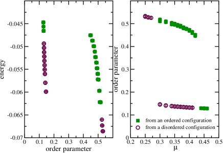
Figure 22: (Color online) Quantum hysteresis — variational Monte Carlo results for $|\psi^{\sf Var}_{\alpha\beta\gamma}\rangle$ [cf. Eq. (20)] in a 1024-bond cluster. (left) energy per site as a function of the order parameter $m_{\sf R}$, (right) order parameter as a function of $\mu$. Simulations converge to different local minima for a range of values of $0.28<\mu<0.43$, according to whether they are started from an ordered or a disordered state.

We can construct another simple one-parameter variational wave function based on the order parameter $m_{\sf R}$ for the R-state

$$|\psi^{\sf Var}_{\beta}\rangle_{\phi,{\sf c}}=\exp[\beta m_{\sf R}]|\psi_{\text{RK}}\rangle_{\phi,{\sf c}}$$ (32)

This wave function gives a good account of the ordered R-state, and exhibits a clear first order phase transition transition from as a jump in $\langle m_{\sf R}\rangle$ for $\mu\approx 0.25$ in a 1024-bond cubic cluster — cf. Fig. 21(a). However from Fig. 21(b) we can see that $|\psi^{\sf Var}_{\alpha}\rangle$ has a lower energy approaching the RK point.

Seeking the advantages of both terms, we try a two-parameter wave function

$$|\psi^{\sf Var}_{\alpha\beta}\rangle_{\phi,{\sf c}}=\exp[\alpha{\mathcal{N}}_{\sf f}+\beta m_{\sf R}]|\psi_{\text{RK}}\rangle_{\phi,{\sf c}}$$ (33)

This gives lower energies overall, and predicts a transition from solid to liquid for $\mu\approx 0.2$ in a (1024 bonds). However this wave function does a poor job of describing the quantum melting of the R-state.

In order to better model this, we introduce correlations between individual flippable plaquettes, on which all dynamics in the QDM depend

$$|\psi^{\sf Var}_{\alpha\beta\gamma}\rangle_{\phi,{\sf c}}=\exp[\alpha{\mathcal{N}}_{\sf f}+\beta m_{\sf R}+\sum_{ij}\gamma_{ij}\tau_{i}\tau_{j}]|\psi_{\text{RK}}\rangle_{\phi,{\sf c}}$$

Here $\tau_{i}=1$ if the plaquette $i$ is flippable and $\tau_{i}=0$, otherwise. For complete generality we should also allow for the chirality of the flippable plaquette, and consider a separate $\gamma_{ij}$ for each indistinguishable pair of plaquettes in the cluster. For the smallest 128 bond cluster there are 16 of these, and the number grows to 84 in the 1024-bond cluster. However in practice we do not find that including chirality brings significant gains in energy, and we restrict our calculations to a set of about 40 $\gamma_{ij}$.

This wave function has a significantly lower energy than any of the alternatives considered above for $-0.5<\mu<0.25$, and predicts a transition for $\mu\approx 0.4$ (1024-bond cluster — black lines in Fig. 21). The wave function also treats fluctuations accurately enough to capture some a part of the hysteresis associated the quantum melting of a solid. In Fig. 22 we show the order parameter and energy for the 1024-bond cluster, obtained using $|\psi^{\sf Var}_{\alpha\beta\gamma}\rangle$, seeding VMC from different states. Starting from an ordered state, we obtain an ordered state solution for $\mu\lesssim 0.42$, while starting from a disordered configuration we could see a minimum for $\mu\gtrsim 0.3$. These results confirm the first order character of the phase transition, and extend the usefulness of $|\psi^{\sf Var}_{\alpha\beta\gamma}\rangle$ as a guide function for GFMC some way into the region where it predicts a liquid phase.

Appendix D Series expansion about the ordered R-state

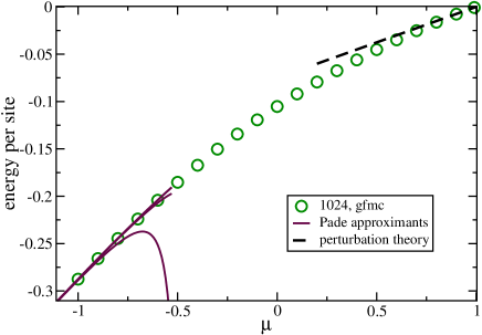
Figure 23: (Color online) Energy per site as a function of $\mu$. GFMC results for 1024-bond cluster (points) are compared to Pade approximants for series expansion around an ordered state (solid lines) and perturbation expansion in the vicinity of the RK point (dashed lines).

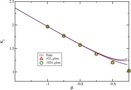
Figure 24: (Color online) Monopole string tension $\kappa_{1}=\Delta_{1}/L$, plotted for a range of $\mu$ spanning the ordered R-state phase. Solid lines denote different Padé approximants to the series expansion about an R-state configuration [cf. Eq. (36)]. Points denote the results of GFMC simulations of 432-bond (red) and 1024-bond (green) cubic clusters.

There are two limits in which the exact ground state of Eq. (1) is known. One is the RK point $\mu=1$, where the ground state is the equally weighted sum over all dimer configurations. The other is $\mu\to-\infty$, where the ground state is one of eight degenerate R-state configurations. In the second case we can construct a perturbation theory in $1/\mu$ by expanding fluctuations about an ordered R-state. We find that the ground state energy (per bond) in the zero-flux sector behaves as

$$\frac{E_{0}}{N} = \frac{\mu}{4}+\frac{1}{24}\frac{1}{\mu}-\frac{229}{47520}\frac{1}{\mu^{3}}$$ (35)

$$+\frac{37811909}{48926592000}\frac{1}{\mu^{5}}+{\mathcal{O}}\left(\frac{1}{\mu^{7}}\right)\;.$$

The first term in this expansion counts the number of flippable plaquettes in the R-state (a quarter of the number of bonds). Subsequent terms are derived combinatorially, by counting the number of possible ways of returning to the the initial R-state, using a given number of applications of ${\mathcal{K}}_{\sf f}$ and following the recipe of the Rayleigh-Schödinger perturbation theory. This can be calculated for a finite-size cluster, or an infinite lattice; the results quoted here are for an infinite lattice. The resulting series Eq. (35) contains only terms of odd order in $1/\mu$.

The series for $E_{0}/N$ [Eq. (35)] can be continued to values of $\mu$ relevant to our simulations by means of Padé approximants. In Fig. 23 we compare several different Padé approximants to Eq. (35), with the ground state energy per bond found in GFMC simulations of a 1024-bond cluster. We find essentially perfect agreement between our simulations results and the results of perturbation theory for $\mu\lesssim-0.8$, at which point the different Padé approximants start to diverge. Some of the Padé approximants remain in agreement with the simulations up to $\mu\approx-0.5$. For comparison, we also include results for $E_{0}/N$ derived in an expansion about the RK point, as described in Section III.4. Again, the agreement between perturbation theory and simulation is found to be very good in the limit $\mu\to 1$.

For $\mu\to-\infty$, it is also possible to perform a series about a state with unit-flux, i.e. an R-state with a single string excitation. From Eq. (21) we find the monopole string tension to be

$$\kappa_{1} = -2\mu+\frac{1}{15}\frac{1}{\mu}-\frac{71243}{1995840}\frac{1}{\mu^{3}}$$ (36)

$$+\frac{1044561213049}{41535007113600000}\frac{1}{\mu^{5}}+{\mathcal{O}}\left(\mu^{-7}\right)\;.$$

In Fig. 24 we compare the perturbational expansion and GFMC simulation results for the string tension $\kappa_{1}$. The prediction of the perturbation theory for $\mu\lesssim-1$ matches well to the results of simulations for $\mu\gtrsim-1$.

References

- (1) M. E. Fisher, Phys. Rev. 124, 1664 (1961)
- (2) P. W. Kastelyn, Physica 27, 1209 (1961)
- (3) D. S. Rokhsar and S. A. Kivelson, Phys. Rev. Lett. 61,2376 (1988).
- (4) G. Misguish and C. Lhuillier, in Frustrated Spin Systems, Ed H. T. Diep, World Scientific, Singapore (2004).
- (5) R. Moessner and S. L. Sondhi, Phys. Rev. Lett. 86, 1881 (2001).
- (6) G. Misguich, D. Serban and V. Pasquier, Phys. Rev. Lett. 89, 137202 (2002).
- (7) D. A. Huse, W. Krauth, R. Moessner, and S. L. Sondhi, Phys. Rev. Lett. 91, 167004 (2003).
- (8) R. Moessner and S. L. Sondhi, Phys. Rev. B 68,184512 (2003).
- (9) P. W. Leung, K. C. Chiu and K. J. Runge, Phys. Rev. B 54, 12938 (1996).
- (10) F. Trousselet, D. Poilblanc and R. Moessner, Phys. Rev. B 78, 195101 (2008)
- (11) R. Moessner, S. L. Sondhi and P. Chandra, Phys. Rev. B 64, 144416 (2001).
- (12) D. L. Bergman, G. A. Fiete, and L. Balents, Phys. Rev. B 73 134402 (2006).
- (13) M. Hermele, M. P. A. Fisher, and L Balents, Phys. Rev. B 69, 064404 (2004).
- (14) O. Sikora, F. Pollmann, N. Shannon, K. Penc, and P. Fulde Phys. Rev. Lett. 103, 247001 (2009).
- (15) P. Fulde, K. Penc and N. Shannon, Ann. Phys. (Leipzig) 11, 892 (2002)
- (16) A. Banerjee, S. V. Isakov, K. Damle, and Y. B. Kim, Phys. Rev. Lett. 100, 047208 (2008).
- (17) J. F. Nagle, Phys. Rev. 152, 190 (1966); J. Math. Phys. 7, 1485 (1966)
- (18) D. L. Bergman, R. Shindou, G. A. Fiete, and L. Balents, Phys. Rev. Lett 96 097207 (2006); erratum ibid 97, 139906 (2006)
- (19) J. Ruostekoski, Phys. Rev. Lett. 103, 080406 (2009)
- (20) F. Vernay, A. Ralko, F. Becca, and F. Mila, Phys. Rev. B 74, 054402 (2006).
- (21) R. Youngblood, J. D. Axe, and B. M. McCoy, Phys. Rev. B 21, 5212 (1980).
- (22) C. L. Henley, Phys. Rev. B 71, 014424 (2005).
- (23) S. V. Isakov, R. Moessner and S. L. Sondhi, Phys. Rev. Lett. 95, 217201 (2005).
- (24) C. L. Henley, Annual Review of Condensed Matter Physics 1, 179 (2010).
- (25) T. Fennel, P. P. Deen, A. R. Wildes, K. Schmalzl, D. Prabhakaran, A. T. Boothroyd, R. J. Aldus, D. F. McMorrow and S. T. Bramwell, Science 326, 415 (2009)
- (26) N. Trivedi and D. M. Ceperley, Phys. Rev. B 41, 4552 (1990).
- (27) M. Calandra Buonaura and S. Sorella, Phys. Rev. B 57,11446 (1998).
- (28) A. Ralko, M. Ferrero, F. Becca, D. Ivanov, and F. Mila, Phys. Rev. B. 71, 224109 (2005).
- (29) A. Ralko, M. Ferrero, F. Becca, D. Ivanov, and F. Mila, Phys. Rev. B. 74, 134301 (2006).
- (30) A. Ralko, M. Ferrero, F. Becca, D. Ivanov, and F. Mila, Phys. Rev. B 76, 140404(R) (2007).
- (31) S. Sorella, Phys. Rev. B 64, 024512 (2001).
- (32) A. Ralko, D. Poilblanc, and R. Moessner, Phys. Rev. Lett 100, 037201 (2008)
- (33) N. Shannon, G. Misguich and K. Penc, Phys. Rev. B 69, 220403(R) (2004)
- (34) O. Sikora, N. Shannon, F. Pollmann, K. Penc, and P. Fulde, unpublished.
- (35) D. Schwandt, M. Mambrini, and D. Poilblanc Phys. Rev. B 81, 214413 (2010).
- (36) M. E. J. Newman and G.T. Barkema, Monte Carlo Methods in Statistical Physics, Clarendon Press, Oxford (2007).
- (37) G.T. Barkema and M. E. J. Newman, Phys. Rev. E 57, 1155 (1998).
- (38) N. Shannon, O. Sikora, F. Pollmann, K. Penc, and P. Fulde, arXiv:1105.4196
- (39) F. Alet, G. Misguich, V. Pasquier, R. Moessner, and J. L. Jacobsen Phys. Rev. Lett. 97, 030403 (2006).
- (40) S. Powell and J. T. Chalker Phys. Rev. Lett. 101, 155702 (2008)
- (41) G. Chen, J. Gukelberger, S. Trebst, F. Alet, and L. Balents, Phys. Rev. B 80, 045112 (2009).
- (42) M. Capello, F. Becca, M. Fabrizio, S. Sorella and E. Tosatti, Phys. Rev. Lett. 94, 026406 (2005).