Intersection Theory on Abelian-Quotient $V$-Surfaces and Q-Resolutions

Abstract.

In this paper we study the intersection theory on surfaces with abelian quotient singularities and we derive properties of quotients of weighted projective planes. We also use this theory to study weighted blow-ups in order to construct embedded Q-resolutions of plane curve singularities and abstract Q-resolutions of surfaces.

Introduction

Intersection theory is a powerful tool in complex algebraic (and analytic) geometry, see [5] for a wonderful exposition. The case of smooth surfaces is of particular interest since the intersection of objects is measured by integers.

The main objects involved in intersection theory on surfaces are divisors, which have two main incarnations, Weil and Cartier. These coincide in the smooth case, but not in general. In the singular case the two concepts are different and a geometric interpretation of intersection theory is yet to be developed. A general definition for normal surfaces was given by Mumford [11].

In this work we are interested in the intersection theory on $V$-surfaces with abelian quotient singularities. We make use of our result in [1], where we proved that the concepts of rational Weil and Cartier divisors coincide. We will study their geometric properties and prove that the definition in this paper coincides with Mumford’s one. The most interesting points are the applications.

Probably the most well-known $V$-surfaces are the weighted projective planes. We will provide an extensive study of intersection theory on these planes and on their quotients.

Closely related with the weighted projective planes we have the weighted blow-ups. As opposed to standard ones, these blow-ups do not produce smooth varieties, but the result may only have abelian quotient singularities. They can be used to understand the birational properties of quotients of weighted projective planes and also to obtain the so-called Q-resolutions of singularities, where the usual conditions are weakened: we allow the total space to have abelian quotient singularities and the condition of normal crossing divisors is replaced by $\mathbb{Q}$-normal crossing divisors. One of the main interest of Q-resolutions of singularities is the following: their combinatorial complexity is extremely lower than the complexity of smooth resolutions, but they provide essentially the same information for the properties of the singularity.

Note that Veys has already studied this kind of embedded resolutions for plane curve singularities, see [15], in order to simplify the computation of the topological zeta function.

In both applications, we need intersection theory. Note that rational intersection numbers appear in a natural way.

Acknowledgements. We thank J.I. Cogolludo for his fruitful conversations and ideas. All authors are partially supported by the Spanish projects MTM2010-2010-21740-C02-02 and “E15 Grupo Consolidado Geometría” from the government of Aragón. Also, the second author, J. Martín-Morales, is partially supported by FQM-333, Junta de Andalucía.

1. $V$-Manifolds and Quotient Singularities

We sketch some definitions and properties, see [1] for a more detailed exposition.

Definition 1.1.

A $V$-manifold of dimension $n$ is a complex analytic space which admits an open covering $\{U_{i}\}$ such that $U_{i}$ is analytically isomorphic to $B_{i}/G_{i}$ where $B_{i}\subset\mathbb{C}^{n}$ is an open ball and $G_{i}$ is a finite subgroup of $GL(n,\mathbb{C})$.

The concept of $V$-manifolds was introduced in [13] and they have the same homological properties over $\mathbb{Q}$ as manifolds. For instance, they admit a Poincaré duality if they are compact and carry a pure Hodge structure if they are compact and K hler, see [2]. They have been classified locally by Prill [12].

It is enough to consider the so-called small subgroups $G\subset\operatorname{GL}(n,\mathbb{C})$, i.e. without rotations around hyperplanes other than the identity.

Theorem 1.2.

([12]). Let $G_{1}$, $G_{2}$ be small subgroups of $\operatorname{GL}(n,\mathbb{C})$. Then $\mathbb{C}^{n}/G_{1}$ is isomorphic to $\mathbb{C}^{n}/G_{2}$ if and only if $G_{1}$ and $G_{2}$ are conjugate subgroups. $\hfill\Box$

We fix the notations when $G$ is abelian.

​​ 1.3.

For $\mathbf{d}:={}^{t}(d_{1}\ldots d_{r})$ we denote $\mu_{\mathbf{d}}:=\mu_{d_{1}}\times\cdots\times\mu_{d_{r}}$ a finite abelian group written as a product of finite cyclic groups, that is, $\mu_{d_{i}}$ is the cyclic group of $d_{i}$-th roots of unity in $\mathbb{C}$. Consider a matrix of weight vectors

$$A:=(a_{ij})_{i,j}=[\mathbf{a}_{1}\,|\,\cdots\,|\,\mathbf{a}_{n}]\in\operatorname{Mat}(r\times n,\mathbb{Z}),\quad\mathbf{a}_{j}:={}^{t}(a_{1j}\dots a_{rj})\in\operatorname{Mat}(r\times 1,\mathbb{Z}),$$

and the action

(1) $$\begin{array}[]{cr}(\mu_{d_{1}}\times\cdots\times\mu_{d_{r}})\times\mathbb{C}^{n}\longrightarrow\mathbb{C}^{n},&\boldsymbol{\xi}_{\mathbf{d}}:=(\xi_{d_{1}},\ldots,\xi_{d_{r}}),\\[4.26773pt] \big{(}\boldsymbol{\xi}_{\mathbf{d}},\mathbf{x}\big{)}\mapsto(\xi_{d_{1}}^{a_{11}}\cdot\ldots\cdot\xi_{d_{r}}^{a_{r1}}\,x_{1},\,\ldots\,,\xi_{d_{1}}^{a_{1n}}\cdot\ldots\cdot\xi_{d_{r}}^{a_{rn}}\,x_{n}),&\mathbf{x}:=(x_{1},\ldots,x_{n}).\end{array}$$

Note that the $i$-th row of the matrix $A$ can be considered modulo $d_{i}$. The set of all orbits $\mathbb{C}^{n}/G$ is called (cyclic) quotient space of type $(\mathbf{d};A)$ and it is denoted by

$$X(\mathbf{d};A):=X\left(\begin{array}[]{c|ccc}d_{1}&a_{11}&\cdots&a_{1n}\\ \vdots&\vdots&\ddots&\vdots\\ d_{r}&a_{r1}&\cdots&a_{rn}\end{array}\right).$$

The orbit of an element $\mathbf{x}\in\mathbb{C}^{n}$ under this action is denoted by $[\mathbf{x}]_{(\mathbf{d};A)}$ and the subindex is omitted if no ambiguity seems likely to arise. Using multi-index notation the action takes the simple form

$$\mu_{\mathbf{d}}\times\mathbb{C}^{n} \longrightarrow \mathbb{C}^{n},$$

$$(\boldsymbol{\xi}_{\mathbf{d}},\mathbf{x}) \mapsto \boldsymbol{\xi}_{\mathbf{d}}\cdot\mathbf{x}:=(\boldsymbol{\xi}_{\mathbf{d}}^{\mathbf{a}_{1}}\,x_{1},\ldots,\boldsymbol{\xi}_{\mathbf{d}}^{\mathbf{a}_{n}}\,x_{n}).$$

The quotient of $\mathbb{C}^{n}$ by a finite abelian group is always isomorphic to a quotient space of type $(\mathbf{d};A)$, see [1] for a proof of this classic result. Different types $(\mathbf{d};A)$ can give rise to isomorphic quotient spaces.

Example 1.4.

When $n=1$ all spaces $X(\mathbf{d};A)$ are isomorphic to $\mathbb{C}$. It is clear that we can assume that $\gcd(d_{i},a_{i})=1$. If $r=1$, the map $[x]\mapsto x^{d_{1}}$ gives an isomorphism between $X(d_{1};a_{1})$ and $\mathbb{C}$.

Let us consider the case $r=2$. Note that $\mathbb{C}/(\mu_{d_{1}}\times\mu_{d_{2}})$ equals $(\mathbb{C}/\mu_{d_{1}})/\mu_{d_{2}}$. Using the previous isomorphism, it is isomorphic to $X(d_{2},d_{1}a_{2})$, which is again isomorphic to $\mathbb{C}$. By induction, we obtain the result for any $r$.

The following lemma states some moves that leave unchanged the isomorphism type of $X(\mathbf{d};A)$.

Lemma 1.5.

The following operations do not change the isomorphism type of $X(\mathbf{d};A)$.

1. Permutation $\sigma$ of columns of $A$, $[(x_{1},\dots,x_{n})]\mapsto[(x_{\sigma(1)},\dots,x_{\sigma(n)})]$.

2. Permutation of rows of $(\mathbf{d};A)$, $[\mathbf{x}]\mapsto[\mathbf{x}]$.

3. Multiplication of a row of $(\mathbf{d};A)$ by a positive integer, $[\mathbf{x}]\mapsto[\mathbf{x}]$.

4. Multiplication of a row of $A$ by an integer coprime with the corresponding row in $\mathbf{d}$, $[\mathbf{x}]\mapsto[\mathbf{x}]$.

5. Replace $a_{ij}$ by $a_{ij}+kd_{j}$, $[\mathbf{x}]\mapsto[\mathbf{x}]$.

6. If $e$ is coprime with $a_{1,n}$ and divides $d_{1}$ and $a_{1,j}$, $1\leq j<n$, then replace, $a_{i,n}\mapsto ea_{i,n}$, $[(x_{1},\dots,x_{n})]\mapsto[(x_{1},\dots,x_{n}^{e})]$.

7. If $d_{r}=1$ then eliminate the last row, $[\mathbf{x}]\mapsto[\mathbf{x}]$.

Using Lemma 1.5 we can prove the following lemma which restricts the number of possible factors of the abelian group in terms of the dimension.

Lemma 1.6.

The space $X(\mathbf{d};A)=\mathbb{C}^{n}/\mu_{d}$ can always be represented by an upper triangular matrix of dimension $(n-1)\times n$. More precisely, there exist a vector ${\bf e}=(e_{1},\ldots,e_{n-1})$, a matrix $B=(b_{i,j})_{i,j}$, and an isomorphism $[(x_{1},\ldots,x_{n})]\mapsto[(x_{1},\ldots,x_{n}^{k})]$ for some $k\in\mathbb{N}$ such that

$$X({\bf d};A)\cong\left(\begin{array}[]{c|cccc}e_{1}&b_{1,1}&\cdots&b_{1,n-1}&b_{1,n}\\ \vdots&\vdots&\ddots&\vdots&\vdots\\ e_{n-1}&0&\cdots&b_{n-1,n-1}&b_{n-1,n}\end{array}\right)=X({\bf e};B).$$

Remark 1.7.

For $n=2$ it is enough to consider cyclic quotients. Nevertheless, in order to avoid cumbersome statements, we will allow if necessary quotients of non-cyclic groups.

As we have already used, if an action is not free on $(\mathbb{C}^{*})^{n}$ we can factor the group by the kernel of the action and the isomorphism type does not change. With all these hypotheses we can define normalized types.

Definition 1.8.

The type $(\mathbf{d};A)$ is said to be normalized if the action is free on $(\mathbb{C}^{*})^{n}$ and $\mu_{\mathbf{d}}$ is small as subgroup of $GL(n,\mathbb{C})$. By abuse of language we often say the space $X(\mathbf{d};A)$ is written in a normalized form when we mean the type $(\mathbf{d};A)$ is normalized.

Proposition 1.9.

The space $X(\mathbf{d};A)$ is written in a normalized form if and only if the stabilizer subgroup of $P$ is trivial for all $P\in\mathbb{C}^{n}$ with exactly $n-1$ coordinates different from zero.

In the cyclic case the stabilizer of a point as above (with exactly $\,n-1$ coordinates different from zero) has order $\gcd(d,a_{1},\ldots,\widehat{a}_{i},\ldots,a_{n})$.

Using Lemma 1.5 it is possible to convert general types $(\mathbf{d};A)$ into their normalized form. Theorem 1.2 allows one to decide whether two quotient spaces are isomorphic. In particular, one can use this result to compute the singular points of the space $X(\mathbf{d};A)$. If $n=2$, then a normalized type is always cyclic.

Definition 1.10.

The index of a quotient $X(\mathbf{d};A)$ of $\mathbb{C}^{2}$ equals $d$ for $X(\mathbf{d};A)\cong X(d;a,b)$ normalized.

In Example 1.4 we have explained the previous normalization process in dimension one. The two and three-dimensional cases are treated in the following examples.

Example 1.11.

Following Lemma 1.6, all quotient spaces for $n=2$ are cyclic. The space $X(d;a,b)$ is written in a normalized form if and only if $\gcd(d,a)=\gcd(d,b)=1$. If this is not the case, one uses the isomorphism (assuming $\gcd(d,a,b)=1$)

$$\begin{array}[]{rcl}X(d;a,b)&\longrightarrow&X\left(\frac{d}{(d,a)(d,b)};\frac{a}{(d,a)},\frac{b}{(d,b)}\right),\\[8.5359pt] \big{[}(x,y)\big{]}&\mapsto&\big{[}(x^{(d,b)},y^{(d,a)})\big{]}\end{array}$$

to convert it into a normalized one, see also Lemma 1.5.

Example 1.12.

The quotient space $X(d;a,b,c)$ is written in a normalized form if and only if $\gcd(d,a,b)=\gcd(d,a,c)=\gcd(d,b,c)=1$. As above, isomorphisms of the form $[(x,y,z)]\mapsto[(x,y,z^{k})]$ can be used to convert types $(d;a,b,c)$ into their normalized form.

Remark 1.13.

Let us show how to convert a space of type $\left(\begin{smallmatrix}p\\ q\end{smallmatrix}\right|\left.\begin{smallmatrix}a&b\\ c&d\end{smallmatrix}\right)$ into its cyclic form. By suitable multiplications of the rows, we can assume $p=q=r$: $X\left(\begin{smallmatrix}r\\ r\end{smallmatrix}\right|\left.\begin{smallmatrix}a&b\\ c&d\end{smallmatrix}\right).$ For the second step we add a third row by adding the first row multiplied by $\alpha$ and the second row multiplied by $\beta$, where $\alpha a+\beta c=m$ and $m:=\gcd(a,c)$ (note that $\gcd(\alpha,\beta)=1$):

$$X\left(\begin{matrix}r\\ r\\ r\end{matrix}\right|\left.\begin{matrix}a&b\\ c&d\\ m&\alpha b+\beta d\end{matrix}\right)=X\left(\begin{matrix}r\\ r\\ r\end{matrix}\right|\left.\begin{matrix}0&-\beta\frac{ad-bc}{m}\\ 0&\alpha\frac{ad-bc}{m}\\ m&\alpha b+\beta d\end{matrix}\right)=X\left(\begin{matrix}r\\ r\end{matrix}\right|\left.\begin{matrix}0&\frac{ad-bc}{m}\\ m&\alpha b+\beta d\end{matrix}\right).$$

Let $t:=\gcd(r,\frac{ad-bc}{m})$. Then, our space is of type $(r;m,(\alpha b+\beta d)\frac{r}{t})$ and normalization follows by taking $\gcd$’s. The isomorphism is $[(x,y)]\mapsto[(x,y^{\frac{r}{t}})]_{(r;m,(\alpha b+\beta d)\frac{r}{t})}$.

In [4] the author computes resolutions of cyclic quotient singularities. In the $2$-dimensional case, the resolution process is due to Jung and Hirzebruch, see [7].

2. Weighted Projective Spaces

The main reference that has been used in this section is [3]. Here we concentrate our attention on the analytic structure.

Let $\omega:=(q_{0},\ldots,q_{n})$ be a weight vector, that is, a finite set of coprime positive integers. There is a natural action of the multiplicative group $\mathbb{C}^{*}$ on $\mathbb{C}^{n+1}\setminus\{0\}$ given by

$$(x_{0},\ldots,x_{n})\longmapsto(t^{q_{0}}x_{0},\ldots,t^{q_{n}}x_{n}).$$

The set of orbits $\frac{\mathbb{C}^{n+1}\setminus\{0\}}{\mathbb{C}^{*}}$ under this action is denoted by $\mathbb{P}^{n}_{\omega}$ (or $\mathbb{P}^{n}(\omega)$ in case of complicated weight vectors) and it is called the weighted projective space of type $\omega$. The class of a nonzero element $(x_{0},\ldots,x_{n})\in\mathbb{C}^{n+1}$ is denoted by $[x_{0}:\ldots:x_{n}]_{\omega}$ and the weight vector is omitted if no ambiguity seems likely to arise. When $(q_{0},\ldots,q_{n})=(1,\ldots,1)$ one obtains the usual projective space and the weight vector is always omitted. For $\mathbf{x}\in\mathbb{C}^{n+1}\setminus\{0\}$, the closure of $[\mathbf{x}]_{\omega}$ in $\mathbb{C}^{n+1}$ is obtained by adding the origin and it is an algebraic curve.

​​ 2.1.

Analytic structure. Consider the decomposition $\mathbb{P}^{n}_{\omega}=U_{0}\cup\cdots\cup U_{n},$ where $U_{i}$ is the open set consisting of all elements $[x_{0}:\ldots:x_{n}]_{\omega}$ with $x_{i}\neq 0$. The map

$$\widetilde{\psi}_{0}:\mathbb{C}^{n}\longrightarrow U_{0},\quad\widetilde{\psi}_{0}(x_{1},\cdots,x_{n}):=[1:x_{1}:\ldots:x_{n}]_{\omega}$$

defines an isomorphism $\psi_{0}$ if we replace $\mathbb{C}^{n}$ by $X(q_{0};\,q_{1},\ldots,q_{n})$. Analogously, $X(q_{i};\,q_{0},\ldots,\widehat{q}_{i},\ldots,q_{n})\cong U_{i}$ under the obvious analytic map.

Proposition 2.2 ([1]).

Let $d_{i}:=\gcd(q_{0},\ldots,\widehat{q}_{i},\ldots,q_{n})$, $e_{i}:=d_{0}\cdot\ldots\cdot\widehat{d}_{i}\cdot\ldots\cdot d_{n}$ and $p_{i}:=\frac{q_{i}}{e_{i}}$. The following map is an isomorphism:

$$\begin{array}[]{rcl}\mathbb{P}^{n}\big{(}q_{0},\ldots,q_{n}\big{)}&\longrightarrow&\mathbb{P}^{n}(p_{0},\dots,p_{n})\\ \,[x_{0}:\ldots:x_{n}]&\mapsto&\big{[}\,x_{0}^{d_{0}}:\ldots:x_{n}^{d_{n}}\,\big{]}.\end{array}$$

Remark 2.3.

Note that, due to the preceding proposition, one can always assume the weight vector satisfies $\gcd(q_{0},\ldots,\widehat{q}_{i},\ldots,q_{n})=1$, for $i=0,\ldots,n$. In particular, $\mathbb{P}^{1}{(q_{0},q_{1})}\cong\mathbb{P}^{1}$ and for $n=2$ we can take $(q_{0},q_{1},q_{2})$ relatively prime numbers. In higher dimension the situation is a bit more complicated.

3. Abstract and Embedded Q-Resolutions

Classically an embedded resolution of $\{f=0\}\subset\mathbb{C}^{n}$ is a proper map $\pi:X\to(\mathbb{C}^{n},0)$ from a smooth variety $X$ satisfying, among other conditions, that $\pi^{-1}(\{f=0\})$ is a normal crossing divisor. To weaken the condition on the preimage of the singularity we allow the new ambient space $X$ to contain abelian quotient singularities and the divisor $\pi^{-1}(\{f=0\})$ to have normal crossings over this kind of varieties. This notion of normal crossing divisor on $V$-manifolds was first introduced by Steenbrink in [14].

Definition 3.1.

Let $X$ be a $V$-manifold with abelian quotient singularities. A hypersurface $D$ on $X$ is said to be with $\mathbb{Q}$-normal crossings if it is locally isomorphic to the quotient of a union of coordinate hyperplanes under a group action of type $(\mathbf{d};A)$. That is, given $x\in X$, there is an isomorphism of germs $(X,x)\simeq(X(\mathbf{d};A),[0])$ such that $(D,x)\subset(X,x)$ is identified under this morphism with a germ of the form

$$\big{(}\{[\mathbf{x}]\in X(\mathbf{d};A)\mid x_{1}^{m_{1}}\cdot\ldots\cdot x_{k}^{m_{k}}=0\},[(0,\ldots,0)]\big{)}.$$

Let $M=\mathbb{C}^{n+1}/\mu_{\mathbf{d}}$ be an abelian quotient space not necessarily cyclic or written in normalized form. Consider $H\subset M$ an analytic subvariety of codimension one.

Definition 3.2.

An embedded Q-resolution of $(H,0)\subset(M,0)$ is a proper analytic map $\pi:X\to(M,0)$ such that:

1. $X$ is a $V$-manifold with abelian quotient singularities.

2. $\pi$ is an isomorphism over $X\setminus\pi^{-1}(\operatorname{Sing}(H))$.

3. $\pi^{-1}(H)$ is a hypersurface with $\mathbb{Q}$-normal crossings on $X$.

Remark 3.3.

Let $f:(M,0)\to(\mathbb{C},0)$ be a non-constant analytic function germ. Consider $(H,0)$ the hypersurface defined by $f$ on $(M,0)$. Let $\pi:X\to(M,0)$ be an embedded Q-resolution of $(H,0)\subset(M,0)$. Then $\pi^{-1}(H)=(f\circ\pi)^{-1}(0)$ is locally given by a function of the form $x_{1}^{m_{1}}\cdot\ldots\cdot x_{k}^{m_{k}}:X(\mathbf{d};A)\rightarrow\mathbb{C}.$

In the same way we define abstract Q-resolutions.

Definition 3.4.

Let $(X,0)$ be a germ of singular point. An abstract good Q-resolution is a proper birational morphism $\pi:\hat{X}\to(X,0)$ such that $\hat{X}$ is a $V$-manifold with abelian quotient singularities, $\pi$ is an isomorphism outside $\operatorname{Sing}(X)$, and $\pi^{-1}(\operatorname{Sing}(X))$ is a $\mathbb{Q}$-normal crossing divisor.

Notation 3.5.

It is usual to encode normal crossing divisors by its dual complex: one vertex for each irreducible component, one edge for each intersection of two irreducible components, one triangle for intersection of three irreducible components and so on. It is particularly useful for normal crossing divisors in surfaces where one deals with (weighted) graphs.

We explain how to encode $\mathbb{Q}$-normal crossings with a weighted graph in the case of surfaces. We are interested in two cases: the divisor $\pi^{*}(H)=(f\circ\pi)^{*}(0)$ for an embedded Q-resolution of a curve $H=f^{*}(0)$ and the exceptional divisor of an abstract good Q-resolution $\pi$ of a normal surface. We associate to such divisors a weighted graph $\Gamma$ as follows:

• The set $V_{\Gamma}$ of vertices of $\Gamma$ is the ordered set of irreducible components of $\pi^{*}(H)$ (for some arbitrary order). It is decomposed in two subsets $V_{\Gamma}=V_{\Gamma}^{0}\coprod V_{\Gamma}^{H}$; the first subset corresponds to exceptional components and the second to strict transforms (using arrow-ends). The set $V_{\Gamma}^{H}$ is empty when the divisor is compact (e.g. when $\pi$ is an abstract good Q-resolution).

• The set $E_{\Gamma}$ of edges of $\Gamma$ is in bijection with the double points of $\pi^{*}(H)$.

• Each $E\in V_{\Gamma}^{0}$ is weighted by its genus $g_{E}$ (usually omitted if $g_{E}=0$. It is also weighted by its self-intersection $e_{E}\in\mathbb{Q}$, see Definition 6.4 later.

• When $\pi$ is an embedded Q-resolution, each $E\in V_{\Gamma}$ is weighted by $m_{E}$. The multiplicity $m_{E}$ is defined as follows: given a generic point in $E$ one can choose local analytic coordinates $(x_{E},y_{E})$ centered at this point such that $y_{E}=0$ is a local equation of $E$ and $(f\circ\pi)(x_{E},y_{E})=y_{E}^{m_{E}}$.

• For $E\in V_{\Gamma}$, let $\operatorname{Sing}^{0}(E)$ be the set of singular points of $\hat{X}$ in $E$ which are not double points. Then, we associate to $E$ the sequenceof normalized types $\{(d_{P};a_{P},b_{P})\}_{P\in\operatorname{Sing}^{0}(E)}$, where for $P\in\operatorname{Sing}^{0}(E)$, $E$ is the image of $y=0$. Note that $d_{P}$ divides $m_{E}$.

• If the double point $P_{\gamma}=E_{1}\cap E_{2}$, $E_{1}<E_{2}$, associated with $\gamma\in E_{\Gamma}$ is singular, we associate to it a normalized type $(d;a,b)$, where $E_{1}$ is the image of $x=0$ and $E_{2}$ is the image of $y=0$. Note that $d$ divides $am_{E_{1}}+bm_{E_{2}}$.

This notation is also useful for exceptional graphs of good Q-resolutions.

4. Weighted Blow-ups

Weighted blow-ups can be defined in any dimension, see [1]. In this section, we restrict our attention to the case $n=2$.

​​ 4.1.

Classical blow-up of $\mathbb{C}^{2}$. We consider

$$\widehat{\mathbb{C}}^{2}:=\big{\{}((x,y),[u:v])\in\mathbb{C}^{2}\times\mathbb{P}^{1}\mid(x,y)\in\overline{[u:v]}\big{\}}.$$

Then $\pi:\widehat{\mathbb{C}}^{2}\to\mathbb{C}^{2}$ is an isomorphism over $\widehat{\mathbb{C}}^{2}\setminus\pi^{-1}(0)$. The exceptional divisor $E:=\pi^{-1}(0)$ is identified with $\mathbb{P}^{1}$. The space $\widehat{\mathbb{C}}^{2}=U_{0}\cup U_{1}$ can be covered with $2$ charts each of them isomorphic to $\mathbb{C}^{2}$. For instance, the following map defines an isomorphism:

$$\mathbb{C}^{2} \longrightarrow U_{0}=\{u\neq 0\}\ \subset\ \widehat{\mathbb{C}}^{2},$$

$$(x,y)\ \mapsto \big{(}(x,xy),[1:y]\big{)}.$$

​​ 4.2.

Weighted $(p,q)$-blow-up of $\mathbb{C}^{2}$. Let $\omega=(p_{0},p_{1})$ be a weight vector with coprime entries. As above, consider the space

$$\widehat{\mathbb{C}}^{2}(\omega):=\big{\{}((x,y),[u:v]_{\omega})\in\mathbb{C}^{2}\times\mathbb{P}^{1}_{\omega}\mid(x,y)\in\overline{[u:v]}_{\omega}\big{\}}.$$

covered as $\widehat{\mathbb{C}}^{2}_{\omega}=U_{1}\cup U_{2}=X(p;-1,q)\cup X(q;\,p,-1)$ and the charts are given by

$$\begin{array}[]{c|rcl}\text{First chart}&X(p;-1,q)&\longrightarrow&U_{1},\\[2.84544pt] &\,[(x,y)]&\mapsto&((x^{p},x^{q}y),[1:y]_{\omega}).\\ \lx@intercol\hfil\hfil\lx@intercol\\ \text{Second chart}&X(q;\,p,-1)&\longrightarrow&U_{2},\\[2.84544pt] &\,[(x,y)]&\mapsto&((xy^{p},y^{q}),[x:1]_{\omega}).\end{array}$$

The exceptional divisor $E:=\pi_{\omega}^{-1}(0)$ is isomorphic to $\mathbb{P}^{1}_{\omega}$ which is in turn isomorphic to $\mathbb{P}^{1}$ under the map $[x:y]_{\omega}\longmapsto[x^{q}:y^{p}]$. The singular points of $\widehat{\mathbb{C}}^{2}_{\omega}$ are cyclic quotient singularities located at the exceptional divisor of indices $p$ and $q$. They actually coincide with the origins of the two charts and are written in their normalized form.

Let us study now the weighted blow-ups of quotient spaces. The general computations were made in [1] and we specialize here for dimension $2$. We study the $(p,q)$-blow-up of $X(d;a,b)$ (in normalized form) and for simplicity we start with the case $p=a$, $q=b$.

​​ 4.3.

Blow-up of $X(d;p,q)$ with respect to $\omega:=(p,q)$. Let $X:=X(d;p,q)$ in a normalized form, i.e. $\gcd(d,p)=\gcd(d,q)=1$. Denote $\pi:=\pi_{\omega,d}:\widehat{\mathbb{C}}^{2}_{\omega,d}\to X(d;p,q)$ the weighted blow-up at the origin with respect to $\omega=(p,q)$. Following [1], we cover $\widehat{X(d;p,q)}_{\omega,d}$ by two charts. The first one is of type

$$X\left(\begin{array}[]{c|cc}p&-1&q\\ pd&p&pq-qp\\ \end{array}\right)=X\left(\begin{array}[]{c|cc}p&-1&q\\ d&1&0\\ \end{array}\right)\stackrel{{\scriptstyle x\mapsto x^{d}}}{{\cong}}X(p;-d,q).$$

Hence $\widehat{\mathbb{C}}^{2}_{\omega,d}=U_{1}\cup U_{2}=X(p;-d,q)\cup X(q;p,-d)$ and the charts are given by

(2) $$\begin{array}[]{c|rcl}\text{First chart}&X(p;-d,q)&\longrightarrow&U_{1},\\[2.84544pt] &\,\big{[}(x^{d},y)\big{]}&\mapsto&\big{(}[(x^{p},x^{q}y)]_{d},[1:y]_{\omega}\big{)}.\\ \lx@intercol\hfil\hfil\lx@intercol\\ \text{Second chart}&X(q;\,p,-d)&\longrightarrow&U_{2},\\[2.84544pt] &\big{[}(x,y^{d})\big{]}&\mapsto&\big{(}[(xy^{p},y^{q})]_{d},[x:1]_{\omega}\big{)}.\end{array}$$

As above the exceptional divisor $E:=\pi_{\omega}^{-1}(0)$ is identified with $\mathbb{P}^{1}_{\omega}$ which is isomorphic to $\mathbb{P}^{1}$ under the map $[x:y]_{\omega}\longmapsto[x^{q}:y^{p}]$. The singular points of $\widehat{\mathbb{C}}^{2}_{\omega,d}$ are cyclic quotient singularities, they coincide with the origins of the two charts and are written in their normalized form.

(a) Blow-up

(b) $\omega$-blow-up

(c) $\omega$-blow-up of $X(d;p,q)$

Figure 1. Graphs of the blow-ups.

Definition 4.4.

Let $\pi:\widehat{X(\mathbf{d};A)}(\omega)\to X(\mathbf{d};A)$ be the $\omega$-blow-up. Then the total transform $\pi^{*}(H)$, $H:=f^{-1}(0)$, for some $f:X(\mathbf{d};A)\to\mathbb{C}$ holomorphic, decomposes as

$$\pi^{*}(H)=\widehat{H}+mE,$$

where $E:=\pi^{-1}(0)$ is the exceptional divisor of $\pi$, $\widehat{H}:=\overline{\pi^{-1}(H\setminus L)}$ is the strict transform of $H$, and $m$ is the multiplicity of $E$ at a smooth point.

Remark 4.5.

In order to compute multiplicities when looking at multicharts (for quotient spaces) we must be careful with the expressions in coordinates in case the space is represented by a non-normalized type. For instance, if a divisor is locally given by the function $x^{md}:X\left(\begin{smallmatrix}p\\ d\end{smallmatrix}\right|\left.\begin{smallmatrix}-1&q\\ 1&0\end{smallmatrix}\right)\rightarrow\mathbb{C}$, its multiplicity is $m$.

Example 4.6.

Assume $\gcd(p,q)=1$ and $p<q$. Let $f=(x^{p}+y^{q})(x^{q}+y^{p})$ and consider ${\bf C}_{1}=\{x^{p}+y^{q}=0\}$ and ${\bf C}_{2}=\{x^{q}+y^{p}=0\}$ the two irreducible components of $\{f=0\}$.

Let $\pi_{(q,p)}:\widehat{\mathbb{C}}^{2}_{(q,p)}\to\mathbb{C}^{2}$ be the $(q,p)$-weighted blow-up at the origin. The new space has two singular points of type $(q;-1,p)$ and $(p;q,-1)$ located at the exceptional divisor $\mathcal{E}_{1}$. The local equation of the total transform in the first chart is given by the function

$$x^{p(p+q)}(1+y^{q})(x^{q^{2}-p^{2}}+y^{p}):X(q;-1,p)\longrightarrow\mathbb{C},$$

where $x=0$ is the equation of the exceptional divisor and the other factors correspond to the strict transform of ${\bf C}_{1}$ and ${\bf C}_{2}$ (denoted again by the same symbol). Due to the cyclic action, $y^{q}+1=0$ produces only one branch.

Hence $\mathcal{E}_{1}$ has multiplicity $p(p+q)$; it intersects transversally ${\bf C}_{1}$ at a smooth point while it intersects ${\bf C}_{2}$ at a singular point (the origin of the first chart) without normal crossings.

Figure 2. Embedded Q-resolution of $\{(x^{p}+y^{q})(x^{q}+y^{p})=0\}\subset\mathbb{C}^{2}$.

Note that $X(q;-1,p)=X(q;p,-p^{2})=X(q;p,q^{2}-p^{2})$ and we can apply 4.3. Let us consider $\pi_{(p,q^{2}-p^{2}),q}$ the weighted blow-up at the origin of $X(q;-1,p)$ with respect to $(p,q^{2}-p^{2})$,

$$\pi_{(p,q^{2}-p^{2}),q}:\,\widehat{\mathbb{C}}^{2}_{(p,q^{2}-p^{2}),q}\longrightarrow X(q;p,q^{2}-p^{2})=X(q;-1,p).$$

The new space has two singular points of type $(p;-q,q^{2}-p^{2})=(p;-1,q)$ and $(q^{2}-p^{2};p,-q)$. In the first chart, the local equation of the total transform of $x^{p(p+q)}(x^{q^{2}-p^{2}}+y^{p})$ is given by the function

$$x^{p(p+q)}(1+y^{p}):\,X(p;-1,q)\longrightarrow\mathbb{C}.$$

Thus the new exceptional divisor $\mathcal{E}_{2}$ has multiplicity $p(p+q)$ and intersects transversally the strict transform of ${\bf C}_{2}$ at a smooth point. Hence $\pi_{(p,q^{2}-p^{2}),q}\circ\pi_{(q,p)}$ is an embedded Q-resolution of $\{f=0\}\subset\mathbb{C}^{2}$ where all quotient spaces are written in a normalized form. Figure 2 illustrates the whole process and Figure 3 shows the dual graph.

Figure 3. Dual graph of the embedded Q-resolution of $\{(x^{p}+y^{q})(x^{q}+y^{p})=0\}\subset\mathbb{C}^{2}$.

We consider now the general case.

​​ 4.7.

Blow-up of $X(d;a,b)$ with respect to $\omega:=(p,q)$. Let $X=X(d;a,b)$ assumed to be normalized. Let

$$\pi:=\pi_{(d;a,b),\omega}:\,\widehat{X(d;a,b)}_{\omega}\longrightarrow X(d;a,b)$$

be the weighted blow-up at the origin of $X(d;a,b)$ with respect to $\omega=(p,q)$. Then, $\widehat{X(d;a,b)}_{\omega}$ is covered by

$$\widehat{U}_{1}\cup\widehat{U}_{2}=X\left(\begin{array}[]{c|cc}p&-1&q\\ pd&a&pb-qa\end{array}\right)\cup X\left(\begin{array}[]{c|cc}q&p&-1\\ qd&qa-pb&b\end{array}\right)$$

and the charts are given by

$$\begin{array}[]{c|c}\text{First chart}&X\left(\begin{array}[]{c|cc}p&-1&q\\ pd&a&pb-qa\end{array}\right)\ \longrightarrow\ \widehat{U}_{1},\\[14.22636pt] &\,\big{[}(x,y)\big{]}\mapsto\big{[}((x^{p},x^{q}y),[1:y]_{\omega})\big{]}_{(d;a,b)}.\\ \lx@intercol\hfil\hfil\lx@intercol\\ \text{Second chart}&X\left(\begin{array}[]{c|cc}q&p&-1\\ qd&qa-pb&b\end{array}\right)\ \longrightarrow\ \widehat{U}_{2},\\[14.22636pt] &\big{[}(x,y)\big{]}\mapsto\big{[}((xy^{p},y^{q}),[x:1]_{\omega})\big{]}_{(d;a,b)}.\end{array}$$

The exceptional divisor $E=\pi_{(d;a,b),\omega}^{-1}(0)$ is identified with the quotient space $\mathbb{P}^{1}_{\omega}(d;a,b):=\mathbb{P}^{1}_{\omega}/\mu_{d}$ which is isomorphic to $\mathbb{P}^{1}$ under the map

$$\begin{array}[]{rcl}\mathbb{P}^{1}_{\omega}(d;a,b)&\longrightarrow&\mathbb{P}^{1},\\[2.84544pt] \,[x:y]_{\omega,(d;a,b)}&\mapsto&[x^{dq/e}:y^{dp/e}],\end{array}$$

where $e:=\gcd(d,pb-qa)$. Again the singular points are cyclic and correspond to the origins.

Let us apply Remark 1.13 to the preceding charts. Assume the type $(d;a,b)$ is normalized. To normalize these quotient spaces, note that $e=\gcd(d,pb-qa)=\gcd(d,-q+\beta pb)=\gcd(pd,-q+\beta pb)=\gcd(qd,p-qa\mu)$, where $\beta a\equiv\mu b\equiv 1\mod d$.

Then another expressions for the two charts are given below.

(3) $$\begin{array}[]{c|c}\text{First chart}&X\left(\displaystyle\frac{pd}{e};1,\frac{-q+\beta pb}{e}\right)\ \longrightarrow\ \widehat{U}_{1},\\[14.22636pt] &\,\big{[}(x^{e},y)\big{]}\mapsto\big{[}((x^{p},x^{q}y),[1:y]_{\omega})\big{]}_{(d;a,b)}.\\ \lx@intercol\hfil\hfil\lx@intercol\\ \text{Second chart}&X\left(\displaystyle\frac{qd}{e};\frac{-p+\mu qa}{e},1\right)\ \longrightarrow\ \widehat{U}_{2},\\[14.22636pt] &\hskip 4.26773pt\big{[}(x,y^{e})\big{]}\mapsto\big{[}((xy^{p},y^{q}),[x:1]_{\omega})\big{]}_{(d;a,b)}.\end{array}$$

Both quotient spaces are now written in their normalized form. The equation of the charts will be useful to compute multiplicities, see Definition 4.4 and Remark 4.5.

Example 4.8.

Assume $\gcd(p,q)=\gcd(r,s)=1$ and $\frac{p}{q}<\frac{r}{s}$. Let $f=(x^{p}+y^{q})(x^{r}+y^{s})$ and consider ${\bf C}_{1}=\{x^{p}+y^{q}=0\}$ and ${\bf C}_{2}=\{x^{r}+y^{s}=0\}$. Working as in Example 4.6, one obtains Figure 4 representing an embedded Q-resolution of $\{f=0\}\subset\mathbb{C}^{2}$. We start with a $(q,p)$-blow-up and we continue with an $(s,qr-ps)$-blow-up over a point of type $(q;-1,p)$.

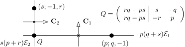
Figure 4. Embedded Q-resolution of $\{(x^{p}+y^{q})(x^{r}+y^{s})=0\}\subset\mathbb{C}^{2}$.

The point $Q$ is also of type $(rq-ps;ar+bs,-1)$ where $ap+bq=1$. In fact, it is in normalized form, since $\gcd(rq-ps,ar+bs)=1$. After writing the quotient spaces in their normalized form one checks that this resolution coincides with the one given in Example 4.6 assuming $r=q$ and $s=p$. The dual graph is shown in Figure 5.

Figure 5. Dual graph of the embedded Q-resolution of $\{(x^{p}+y^{q})(x^{r}+y^{s})=0\}\subset\mathbb{C}^{2}$, $ap+bq=1$.

​​ 4.9.

Puiseux expansion. Let us study the behavior of Puiseux pairs under weighted blow-ups. Let ${\bf C}=\{f=0\}\subset\mathbb{C}^{2}$ be the irreducible plane curve given by

$$\prod_{j=1}^{d}\big{[}-y+(a_{11}x^{\frac{p_{1}}{q}}+\cdots+a_{k1}x^{\frac{p_{k}}{q}})+(a_{12}x^{\frac{r_{1}}{qs}}+\cdots+a_{l2}x^{\frac{r_{l}}{qs}})+\cdots\big{]},$$

where $p_{1}<\cdots<p_{k}$, $r_{1}<\cdots<r_{l}$, $\frac{p_{k}}{q}<\frac{r_{1}}{qs}$, $\gcd(p_{1},q)=\gcd(r_{1},s)=1$, and $q,s>1$ (after a change of variables we may assume the first term has non-integer exponent).

Let $\pi_{(q,p_{1})}:\widehat{\mathbb{C}}^{2}_{(q,p_{1})}\to\mathbb{C}^{2}$ be the $(q,p_{1})$-weighted blow-up at the origin. In the first chart, that is, after performing the substitution $(x,y)\mapsto(x^{q},x^{p_{1}}y)$, one obtains the following equation for the total transform

$$\begin{split}x^{p_{1}d}\cdot\prod_{j=1}^{d}\big{[}-y\,+\,&(a_{11}+a_{21}x^{p_{2}-p_{1}}+\cdots+a_{k1}x^{p_{k}-p_{1}})+\\ &(a_{12}x^{\frac{r_{1}-p_{1}s}{s}}+\cdots+a_{l2}x^{\frac{r_{l}-p_{1}s}{s}})+\cdots\big{]}=0.\end{split}$$

At first sight the exceptional divisor and the strict transform intersect at $d$ different smooth points. However, since $a_{1j}^{q}$ does not depend on $j$ by conjugation, all of them are the same.

After change of coordinates $y\mapsto y+(a_{11}+a_{21}x^{p_{2}-p_{1}}+\cdots+a_{k1}x^{p_{k}-p_{1}}),$ the local equation of the total transform $\pi^{*}_{(q,p_{1})}({\bf C})$ at this point is

$$x^{p_{1}d}\cdot\prod_{j=1}^{d/q}\big{[}-y+(a_{12}x^{\frac{r_{1}-p_{1}s}{s}}+\cdots+a_{l2}x^{\frac{r_{l}-p_{1}s}{s}})+\cdots\big{]}=0.$$

This proves that in the irreducible case, only a weighted blow-up is needed for each Puiseux pair in order to compute an embedded Q-resolution, and the weight is determined by the Puiseux pairs. Moreover, the embedded Q-resolution obtained is as in Figure 6.

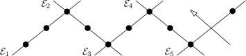
Figure 6. Embedded Q-resolution of an irreducible plane curve.

In the reducible case, one has to consider the weighted blow-ups associated with the Puiseux pairs of each irreducible component and add also weighted blow-ups associated with the contact exponents for each pair of branches. There is another longer way to get this Q-resolution: perform a standard embedded resolution and contract any exceptional component having at most two singular points in the divisor, cf. [15].

Example 4.10.

Let us consider $X:=\mathbb{P}^{2}_{\omega}$, for $\omega=(p,q,r)$. We recall that $P:=[0:1:0]_{\omega}$ is a singular point of type $(q;p,r)$. We are going to perform the $(p,r)$-blow-up at this point. The new surface $\hat{X}_{P}$ admits a map onto $\pi:\hat{X}_{P}\to\mathbb{P}^{1}_{(p,r)}\cong\mathbb{P}^{1}$ with rational fibers. This surface has (at most) four singular points; two of them come from $X$ and they are of type $(p;q,r)$, $Q:=[1:0:0]_{\omega}$, and $(r;p,q)$, $R:=[0:0:1]_{\omega}$. The other two points are in the exceptional divisor $E$ and they are of type $(p;-q,r)$ and $(r;p,-q)$; the singular points which are quotient by $\mu_{p}$ are in the same fiber for $\pi$ and the same happens for $\mu_{r}$. The map has two relevant sections, $E$ and the transform of $y=0$.

5. Cartier and Weil $\mathbb{Q}$-Divisors on $V$-Manifolds

We recall the definitions of Cartier and Weil divisors. Let $X$ be an irreducible normal complex analytic variety. Denote $\mathcal{O}_{X}$ the structure sheaf of $X$ and $\mathcal{K}_{X}$ the sheaf of total quotient rings of $\mathcal{O}_{X}$. Denote by $\mathcal{K}_{X}^{*}$ the (multiplicative) sheaf of invertible elements in $\mathcal{K}_{X}$. Similarly $\mathcal{O}_{X}^{*}$ is the sheaf of invertible elements in $\mathcal{O}_{X}$. Note that an irreducible subvariety $V$ corresponds to a prime ideal in the ring of sections of any local complex model space meeting $V$.

Definition 5.1.

A Cartier divisor on $X$ is a global section of the sheaf $\mathcal{K}_{X}^{*}/\mathcal{O}_{X}^{*}$ and it can be represented by giving an open covering $\{U_{i}\}_{i\in I}$ of $X$ and, for all $i\in I$, an element $f_{i}\in\Gamma(U_{i},\mathcal{K}_{X}^{*})$ such that

$$\frac{f_{i}}{f_{j}}\in\Gamma(U_{i}\cap U_{j},\mathcal{O}_{X}^{*}),\quad\forall i,j\in I.$$

Two systems $\{(U_{i},f_{i})\}_{i\in I}$, $\{(V_{j},g_{j})\}_{j\in J}$ represent the same Cartier divisor if and only if on $U_{i}\cap V_{j}$, $f_{i}$ and $g_{j}$ differ by a multiplicative factor in $\mathcal{O}_{X}(U_{i}\cap V_{j})^{*}$. The abelian group of Cartier divisors on $X$ is denoted by $\operatorname{CaDiv}(X)$. If $D:=\{(U_{i},f_{i})\}_{i\in I}$ and $E:=\{(V_{j},g_{j})\}_{j\in J}$ then $D+E=\{(U_{i}\cap V_{j},f_{i}g_{j})\}_{i\in I,j\in J}$.

The functions $f_{i}$ above are called local equations of the divisor on $U_{i}$. A Cartier divisor on $X$ is effective if it can be represented by $\{(U_{i},f_{i})\}_{i}$ with all local equations $f_{i}\in\Gamma(U_{i},\mathcal{O}_{X})$.

Any global section $f\in\Gamma(X,\mathcal{K}^{*}_{X})$ determines a principal Cartier divisor $(f)_{X}:=\{(X,f)\}$ by taking all local equations equal to $f$. That is, a Cartier divisor is principal if it is in the image of the natural map $\Gamma(X,\mathcal{K}_{X}^{*})\to\Gamma(X,\mathcal{K}_{X}^{*}/\mathcal{O}_{X}^{*})$. Two Cartier divisors $D$ and $E$ are linearly equivalent, denoted by $D\sim E$, if they differ by a principal divisor. The Picard group $\operatorname{Pic}(X)$ denotes the group of linear equivalence classes of Cartier divisors.

The support of a Cartier divisor $D$, denoted by $\operatorname{Supp}(D)$ or $|D|$, is the subset of $X$ consisting of all points $x$ such that a local equation for $D$ is not in $\mathcal{O}_{X,x}^{*}$. The support of $D$ is a closed subset of $X$.

Definition 5.2.

A Weil divisor on $X$ is a locally finite linear combination with integral coefficients of irreducible subvarieties of codimension one. The abelian group of Weil divisors on $X$ is denoted by $\operatorname{WeDiv}(X)$. If all coefficients appearing in the sum are non-negative, the Weil divisor is called effective.

Given a Cartier divisor, using the notion of order of a divisor along an irreducible subvariety of codimension one, there is a Weil divisor associated with it. Let $V\subset X$ be an irreducible subvariety of codimension one. It corresponds to a prime ideal in the ring of sections of any local complex model space meeting $V$. The local ring of $X$ along $V$, denoted by $\mathcal{O}_{X,V}$, is the localization of such ring of sections at the corresponding prime ideal; it is a one-dimensional local domain.

For a given $f\in\mathcal{O}_{X,V}$ define $\operatorname{ord}_{V}(f)$ to be

$$\operatorname{ord}_{V}(f):=\operatorname{length}_{\mathcal{O}_{X,V}}\left(\frac{\mathcal{O}_{X,V}}{\langle f\rangle}\right).$$

This determines a well-defined group homomorphism $\operatorname{ord}_{V}:\Gamma(X,\mathcal{K}_{X}^{*})\to\mathbb{Z}$. This length can be computed as follows. Choose $x\in V$ such that $x$ is smooth in $X$ and $(V,x)$ defines an irreducible germ. This germ is the zero set of an irreducible $g\in\mathcal{O}_{X,x}$. Then $\operatorname{ord}_{V}(f)=\operatorname{ord}_{V,x}(f),$ where $\operatorname{ord}_{V,x}(f)$ is the classical order of a meromorphic function at a smooth point with respect to an irreducible subvariety of codimension one; it is known to be given by the equality $f=g^{\operatorname{ord}}\cdot h\in\mathcal{O}_{X,x}$ where $h\nmid g$.

Now if $D$ is a Cartier divisor on $X$, one writes $\operatorname{ord}_{V}(D)=\operatorname{ord}_{V}(f_{i})$ where $f_{i}$ is a local equation of $D$ on any open set $U_{i}$ with $U_{i}\cap V\neq\emptyset$. This is well defined since $f_{i}$ is uniquely determined up to multiplication by units and the order function is a homomorphism. Define the associated Weil divisor of a Cartier divisor $D$ by

$$\begin{array}[]{cccl}T_{X}:&\operatorname{CaDiv}(X)&\longrightarrow&\operatorname{WeDiv}(X),\\[4.26773pt] &D&\mapsto&\displaystyle\sum_{V\subset X}\operatorname{ord}_{V}(D)\cdot[V],\end{array}$$

where the sum is taken over all codimension one irreducible subvarieties $V$ of $X$; the mapping $T_{X}$ is a homomorphism of abelian groups.

A Weil divisor is principal if it is the image of a principal Cartier divisor under $T_{X}$; they form a subgroup of $\operatorname{WeDiv}(X)$. If $\operatorname{Cl}(X)$ denotes the quotient group of their equivalence classes, then $T_{X}$ induces a morphism $\operatorname{Pic}(X)\rightarrow\operatorname{Cl}(X)$.

These two homomorphisms ($T_{X}$ and the induced one) are in general neither injective nor surjective.

Example 5.3.

Let $X:=X(2;1,1)$ and consider the Weil divisor $D$ associated with $x=0$. Since $x$ does not define a function on $X$, then $D$ is not a Cartier divisor. Since $x^{2}:X(2;1,1)\to\mathbb{C}$, then $E:=\{(X(2;1,1),x^{2})\}$ is a Cartier divisor and it is easily seen that $T_{X}(E)=2D$.

Example 5.3 above illustrates the general behavior of Cartier and Weil divisors on $V$-manifolds. The following theorem allows us to identify both notions on $V$-manifolds after tensorizing by $\mathbb{Q}$.

Theorem 5.4 ([1]).

Let $X$ be a $V$-manifold. Then the notion of Cartier and Weil divisor coincide over $\mathbb{Q}$. More precisely, the linear map

$$T_{X}\otimes 1:\operatorname{CaDiv}(X)\otimes_{\mathbb{Z}}\mathbb{Q}\longrightarrow\operatorname{WeDiv}(X)\otimes_{\mathbb{Z}}\mathbb{Q}$$

is an isomorphism of $\mathbb{Q}$-vector spaces. In particular, for a given Weil divisor $D$ on $X$ there always exists $k\in\mathbb{Z}$ such that $kD\in\operatorname{CaDiv}(X)$.

Definition 5.5.

Let $X$ be a $V$-manifold. The vector space of $\mathbb{Q}$-Cartier divisors is identified under $T_{X}$ with the vector space of $\mathbb{Q}$-Weil divisors. A $\mathbb{Q}$-divisor on $X$ is an element in $\operatorname{CaDiv}(X)\otimes_{\mathbb{Z}}\mathbb{Q}=\operatorname{WeDiv}(X)\otimes_{\mathbb{Z}}\mathbb{Q}.$ The set of all $\mathbb{Q}$-divisors on $X$ is denoted by $\mathbb{Q}$-$\operatorname{Div}(X)$.

In [1], we also give a way to construct the inverse of $T_{X}\otimes 1$.

​​ 5.6.

Here we summarize how to write a Weil divisor as a $\mathbb{Q}$-Cartier divisor where $X$ is an algebraic $V$-manifold.

1. Write $D=\sum_{i\in I}a_{i}[V_{i}]\in\operatorname{WeDiv}(X)$, where $a_{i}\in\mathbb{Z}$ and $V_{i}\subset X$ irreducible. Also choose $\{U_{j}\}_{j\in J}$ an open covering of $X$ such that $U_{j}=B_{j}/G_{j}$ where $B_{j}\subset\mathbb{C}^{n}$ is an open ball and $G_{j}$ is a small finite subgroup of $GL(n,\mathbb{C})$.

2. For each $(i,j)\in I\times J$ choose a reduced polynomial $f_{i,j}:U_{j}\to\mathbb{C}$ such that $V_{i}\cap U_{j}=\{f_{i,j}=0\}$, then

   $$[V_{i}|_{U_{j}}]=\frac{1}{|G_{j}|}\{(U_{j},f_{i,j}^{|G_{j}|})\}.$$

3. Identifying $\{(U_{j},f_{i,j}^{|G_{j}|})\}$ with its image $\operatorname{CaDiv}(U_{j})\hookrightarrow\operatorname{CaDiv}(X),$ one finally writes $D$ as a sum of locally principal Cartier divisors over $\mathbb{Q}$,

   $$D=\sum_{(i,j)\in I\times J}\frac{a_{i}}{|G_{j}|}\{(U_{j},f_{i,j}^{|G_{j}|})\}.$$

Let us apply this procedure to write the exceptional divisor of a weighted blow-up (which is in general just a Weil divisor) as a $\mathbb{Q}$-Cartier divisor.

Example 5.7.

Let $X$ be a surface with abelian quotient singularities. Let $\pi:\widehat{X}\to X$ be the weighted blow-up at a point of type $(d;a,b)$ with respect to $\omega=(p,q)$. In general, the exceptional divisor $E:=\pi^{-1}(0)\cong\mathbb{P}^{1}_{\omega}(d;a,b)$ is a Weil divisor on $\widehat{X}$ which does not correspond to a Cartier divisor. Let us write $E$ as an element in $\operatorname{CaDiv}(\widehat{X})\otimes_{\mathbb{Z}}\mathbb{Q}$.

As in 4.7, assume $\pi:=\pi_{(d;a,b),\omega}:\widehat{X(d;a,b)}_{\omega}\to X(d;a,b)$. Assume also that $\gcd(p,q)=1$ and $(d;a,b)$ is normalized. Using the notation introduced in 4.7, the space $\widehat{X}$ is covered by $\widehat{U}_{1}\cup\widehat{U}_{2}$ and the first chart is given by

(4) $$\begin{array}[]{rcl}Q_{1}:=X\Big{(}\frac{pd}{e};1,\frac{-q+\beta pb}{e}\Big{)}&\longrightarrow&\widehat{U}_{1},\\[7.11317pt] \,\big{[}(x^{e},y)\big{]}&\mapsto&\big{[}((x^{p},x^{q}y),[1:y]_{\omega})\big{]}_{(d;a,b)},\end{array}$$

where $e:=\gcd(d,pb-qa)$, see 4.7 for details.

In the first chart, $E$ is the Weil divisor $\{x=0\}\subset Q_{1}$. Note that the type representing the space $Q_{1}$ is in a normalized form and hence the corresponding subgroup of $GL(2,\mathbb{C})$ is small.

Following the discussion 5.6, the divisor $\{x=0\}\subset Q_{1}$ is written as an element in $\operatorname{CaDiv}(Q_{1})\otimes_{\mathbb{Z}}\mathbb{Q}$ like $\frac{e}{pd}\{(Q_{1},x^{\frac{pd}{e}})\}$, which is mapped to $\frac{e}{pd}\{(\widehat{U}_{1},x^{d})\}\in\operatorname{CaDiv}(\widehat{U}_{1})\otimes_{\mathbb{Z}}\mathbb{Q}$ under the isomorphism (4).

Analogously $E$ in the second chart is $\frac{e}{qd}\{(\widehat{U}_{2},y^{d})\}$. Finally one writes the exceptional divisor of $\pi$ as claimed,

$$E=\frac{e}{dp}\big{\{}(\widehat{U}_{1},x^{d}),(\widehat{U}_{2},1)\big{\}}+\frac{e}{dq}\big{\{}(\widehat{U}_{1},1),(\widehat{U}_{2},y^{d})\big{\}}=\frac{e}{dpq}\big{\{}(\widehat{U}_{1},x^{dq}),(\widehat{U}_{2},y^{dp})\big{\}}.$$

​​ 5.8.

Cartier divisors and sections of line bundles. Given a line bundle $\pi:E\to X$ and a non-zero meromorphic section $s:X\dashrightarrow E$, a Cartier divisor $\operatorname{Div}(s)$ can be constructed using the expression of $s$ in charts. By its very construction, a line bundle $\mathcal{O}(D)$ is associated with a Cartier divisor $D=\{(U_{i},f_{i})\}_{i\in I}$; moreover one can also associate a class of meromorphic sections $S_{D}:=\{s_{D}:X\dasharrow\mathcal{O}(D)\mid\operatorname{Div}(s_{D})=D\}$; once such a section is constructed any other one in $S_{D}$ is obtained by multiplying by an element in $\Gamma(X,\mathcal{O}_{X}^{*})$. A divisor is effective if the sections in $S_{D}$ are holomorphic.

Let $F:Y\to X$ be a morphism between two irreducible complex analytic varieties. The pull-back of a Cartier divisor $D=\{(U_{i},f_{i})\}_{i\in I}$ on $X$ is defined by pulling back the local equations of $D$ as

$$F^{*}(D)=\big{\{}(F^{-1}(U_{i}),f_{i}\circ F|_{F^{-1}(U_{i})}\big{\}}_{i\in I}$$

and it is a Cartier divisor on $Y$ provided $F(Y)\nsubseteq\operatorname{Supp}(D)$. If $F(Y)\subset\operatorname{Supp}(D)$ then we identify $F^{*}(Y)$ with $F^{*}\mathcal{O}(D)$. If this line bundle admits nonzero meromorphic sections we consider $F^{*}(Y)$ as a linear equivalence class of Cartier Divisors. Moreover, $F^{*}$ respects sums of divisors and preserves linear equivalence. In the same way, pull-backs of $\mathbb{Q}$-Cartier divisors can be defined. Note that $F^{*}\mathcal{O}(D)=\mathcal{O}(F^{*}D)$ and the same happens for sections.

Remark 5.9.

Line bundles on projective varieties admit nonzero meromorphic sections. It is also the case for a ball $B\subset\mathbb{C}^{n}$ since only the trivial bundle can be constructed.

By the results in this section the pull-back of a Weil divisor can be also constructed for $V$-manifolds.

6. Rational Intersection Number on $V$-Surfaces: Generalities

Now we have all the necessary ingredients to develop a rational intersection theory on varieties with quotient singularities. This section is devoted to working out all the details, but the following illustrative example will be given.

Example 6.1.

Let $X:=X(2;1,1)$ and consider the Weil divisors $D_{1}:=\{x=0\}$ and $D_{2}:=\{y=0\}$. Let us compute the Weil divisor associated with $j^{*}_{D_{1}}D_{2}$, where $j_{D_{1}}:|D_{1}|\hookrightarrow X$ is the inclusion. Following 5.6, the divisor $D_{2}$ can be written as $\frac{1}{2}\{(X,y^{2})\}$. By definition, since $|D_{1}|\nsubseteq|D_{2}|$, the pull-back is $j^{*}_{D_{1}}D_{2}=\frac{1}{2}\big{\{}(D_{1},y^{2}|_{D_{1}})\big{\}},$ and its associated Weil divisor is

$$T_{D_{1}}(j^{*}_{D_{1}}D_{2})=\frac{1}{2}\sum_{P\in D_{1}}\operatorname{ord}_{P}(y^{2}|_{D_{1}})\cdot[P]=\frac{1}{2}\operatorname{ord}_{[(0,0)]}(y^{2}|_{D_{1}})\cdot[(0,0)]\ =\ \frac{1}{2}\cdot[(0,0)].$$

Note that there is an isomorphism $D_{1}=X(2;1)\simeq\mathbb{C}$, $[y]\mapsto y^{2}$, and the function $y^{2}:D_{1}\to\mathbb{C}$ is converted into the identity map $\mathbb{C}\to\mathbb{C}$ under this isomorphism. Hence $\operatorname{ord}_{[(0,0)]}(y^{2}|_{D_{1}})=1$. It is natural to define the (global and local) intersection multiplicity as $D_{1}\cdot D_{2}=(D_{1}\cdot D_{2})_{[(0,0)]}=\frac{1}{2}.$

Definition 6.2.

Let $\mathcal{C}$ be an irreducible analytic curve. Given a Weil divisor on $\mathcal{C}$ with finite support, $D:=\sum_{i=1}^{r}n_{i}\cdot[P_{i}]$, its degree is defined as $\deg(D)=\sum_{i=1}^{r}n_{i}\in\mathbb{Z}$. The degree of a Cartier divisor is the degree of its associated Weil divisor, that is, by definition $\deg(D):=\deg(T_{\mathcal{C}}D)$.

The degree map is a group homomorphism. If $\mathcal{C}$ is compact, the degree of a principal divisor is zero and thus passes to the quotient yielding $\deg:\operatorname{Cl}(\mathcal{C})\to\mathbb{Z}$, cf. [5, Prop. 1.4].

Definition 6.3.

Let $X$ be an analytic surface and consider $D_{1}\in\operatorname{WeDiv}(X)$ and $D_{2}\in\operatorname{CaDiv}(X)$. If $D_{1}$ is irreducible, then the intersection number is defined as

$$D_{1}\cdot D_{2}:=\deg(j_{D_{1}}^{*}D_{2})\in\mathbb{Z},$$

where $j_{D_{1}}\hookrightarrow X$ denotes the inclusion and $j_{D_{1}}^{*}$ its pull-back functor. The expression above extends linearly if $D_{1}$ is a finite sum of irreducible divisors. This intersection number is only well defined if $D_{1}\nsubseteq D_{2}$ and $D_{1}\cap D_{2}$ is finite, or if the divisor $D_{1}$ is compact, cf. [5, Ch. 2].

In the case $D_{1}\nsubseteq D_{2}$ the number $(D_{1}\cdot D_{2})_{P}:=\operatorname{ord}_{P}(j_{D_{1}}^{*}D_{2})$ with $P\in D_{1}\cap D_{2}$ is well defined too and it is called local intersection number at $P$.

Definition 6.4.

Let $X$ be a $V$-manifold of dimension $2$ and consider $D_{1},D_{2}\in\mathbb{Q}$-$\operatorname{Div}(X)$. The intersection number is defined as

$$D_{1}\cdot D_{2}:=\frac{1}{k_{1}k_{2}}(k_{1}D_{1}\cdot k_{2}D_{2})\in\mathbb{Q},$$

where $k_{1},k_{2}\in\mathbb{Z}$ are chosen so that $k_{1}D_{1}\in\operatorname{WeDiv}(X)$ and $k_{2}D_{2}\in\operatorname{CaDiv}(X)$. Analogously, it is defined the local intersection number at $P\in D_{1}\cap D_{2}$, if the condition $D_{1}\nsubseteq D_{2}$ is satisfied. Idem the pull-back is defined by $F^{*}(D_{1}):=\frac{1}{k_{1}}(k_{1}D_{1})$ if $F:Y\to X$ is a proper morphism between two irreducible $V$-surfaces.

Remark 6.5.

If $D_{1}\nsubseteq D_{2}$ and $D_{1}\cap D_{2}$ is finite, then the global and the local intersection number at $P\in D_{1}\cap D_{2}$ are defined, and indeed by definition

$$D_{1}\cdot D_{2}=\displaystyle\sum_{P\in D_{1}\cap D_{2}}(D_{1}\cdot D_{2})_{P}.$$

In the following result the main usual properties of the intersection multiplicity are collected. Their proofs are omitted since they are well known for the classical case (i.e. without tensoring with $\mathbb{Q}$), cf. [5], and our generalization is based on extending the classical definition to rational coefficients.

Proposition 6.6.

Let $X$ be a $V$-manifold of dimension $2$ and $D_{1},D_{2},D_{3}\in\mathbb{Q}$-$\operatorname{Div}(X)$. Then the local and the global intersection numbers, provided the indicated operations make sense according to Definition 6.4, satisfy the following properties: ($\alpha\in\mathbb{Q}$, $P\in X$)

1. The intersection product is bilinear over $\mathbb{Q}$.

2. Commutative: If $D_{1}\cdot D_{2}$ and $D_{2}\cdot D_{1}$ are both defined, then $D_{1}\cdot D_{2}=D_{2}\cdot D_{1}$. Analogously $(D_{1}\cdot D_{2})_{P}=(D_{2}\cdot D_{1})_{P}$ if both local numbers are defined.

3. Non-negative: Assume $D_{1}$ and $D_{2}$ are effective, irreducible and distinct. Then $D_{1}\cdot D_{2}$ and $(D_{1}\cdot D_{2})_{P}$ are greater than or equal to zero if they are defined. Moreover, $(D_{1}\cdot D_{2})_{P}=0$ if and only if $P\notin|D_{1}|\cap|D_{2}|$, and hence $D_{1}\cdot D_{2}=0$ if and only if $|D_{1}|\cap|D_{2}|=\emptyset$.

4. Non-rational: If $D_{2}\in\operatorname{CaDiv}(X)$ and $D_{1}\in\operatorname{WeDiv}(X)$ then $D_{1}\cdot D_{2}$ and $(D_{1}\cdot D_{2})_{P}$ are integral numbers. By the commutative property, the same holds if $D_{1}$ is a Cartier divisor and $D_{2}$ is a Weil divisor.

5. $\mathbb{Q}$-Linear equivalence: Assume $D_{1}$ has compact support. If $D_{2}$ and $D_{3}$ are $\mathbb{Q}$-linearly equivalent, i.e. $[D_{2}]=[D_{3}]\in\operatorname{Pic}(X)\otimes_{\mathbb{Z}}\mathbb{Q}$, then $D_{1}\cdot D_{2}=D_{1}\cdot D_{3}$. Due to the commutativity, the roles of $D_{1}$ and $D_{2}$ can be exchanged. In particular $D_{1}\cdot D_{2}=0$ for every principal $\mathbb{Q}$-divisor $D_{2}$.

6. Normalization: Let $\nu:\widetilde{|D_{1}|}\to|D_{1}|$ be the normalization of the support of $D_{1}$ and $j_{D_{1}}:|D_{1}|\hookrightarrow X$ the inclusion. Then $D_{1}\cdot D_{2}=\deg\big{(}j_{D_{1}}\circ\nu\big{)}^{*}D_{2}$. Observe that in this situation the normalization is a smooth complex analytic curve.

Remark 6.7.

This rational intersection multiplicity was first introduced by Mumford for normal surfaces, see [11, Pag. 17]. Our Definition 6.4 coincides with Mumford’s because it has good behavior with respect to the pull-back, see Theorem 6.8 and a direct proof will be also given later, see Proposition 7.8. The main advantage is that ours does not involve a resolution of the ambient space and, for instance, this allows us to easily find formulas for the self-intersection numbers of the exceptional divisors of weighted blow-ups, without computing any resolution, see Proposition 7.3.

Theorem 6.8.

Let $F:Y\to X$ be a proper morphism between two irreducible $V$-manifolds of dimension $2$, and $D_{1},D_{2}\in\mathbb{Q}$-$\operatorname{Div}(X)$.

1. The cardinal of $F^{-1}(P)$, $P\in X$ being generic, is a finite constant. This number is denoted by $\deg(F)$.

2. If $D_{1}\cdot D_{2}$ is defined, then so is the number $F^{*}(D_{1})\cdot F^{*}(D_{2})$. In such a case $F^{*}(D_{1})\cdot F^{*}(D_{2})=\deg(F)\,(D\cdot E)$.

3. If $(D_{1}\cdot D_{2})_{P}$ is defined for some $P\in X$, then so is $(F^{*}(D_{1})\cdot F^{*}(D_{2}))_{Q}$, $\forall Q\in F^{-1}(P)$, and $\sum_{Q\in F^{-1}(P)}(F^{*}(D_{1})\cdot F^{*}(D_{2}))_{Q}=\deg(F)(D_{1}\cdot D_{2})_{P}$.

The rest of this section is devoted to reviewing some classical results concerning the intersection multiplicity, namely, the computation of the local intersection number at a smooth point, the self-intersection numbers of the exceptional divisors of blow-ups at a smooth point, and the classical Bézout’s Theorem on $\mathbb{P}^{2}$. Afterwards, these results are generalized in the upcoming sections.

​​ 6.9.

Local intersection number at a smooth point. Let $X$ be a smooth analytic surface. Consider $D_{1}$, $D_{2}$ two effective (Cartier or Weil) divisors on $X$ and $P\in X$ a point. The divisor $D_{i}$ is locally given by a holomorphic function $f_{i}$, $i=1,2$, in a neighborhood of $P$. Then $(D_{1}\cdot D_{2})_{P}$ equals

$$\operatorname{ord}_{P}(f_{2}|D_{1})=\operatorname{length}_{\mathcal{O}_{D_{1},P}}\left(\frac{\mathcal{O}_{D_{1},P}}{f_{2}|_{D_{1}}}\right)=\dim_{\mathbb{C}}\left(\frac{\mathcal{O}_{X,P}}{\langle f_{1},f_{2}\rangle}\right).$$

Moreover, $X$ being a smooth variety, $\mathcal{O}_{X,P}$ is isomorphic to $\mathbb{C}\{x,y\}$ and hence the previous dimension can be computed, for instance, by means of Gr bner bases with respect to local orderings.

​​ 6.10.

Classical blow-up at a smooth point. Let $X$ be a smooth analytic surface. Let $\pi:\widehat{X}\to X$ be the classical blow-up at a (smooth) point $P$. Consider $C$ and $D$ two (Cartier or Weil) divisors on $X$ with multiplicities $m_{C}$ and $m_{D}$ at $P$. Denote by $E$ the exceptional divisor of $\pi$, and by $\widehat{C}$ (resp. $\widehat{D}$) the strict transform of $C$ (resp. $D$). Then,

1. $E\cdot\pi^{*}(C)=0$,   $\pi^{*}(C)=\widehat{C}+m_{C}E$,   $E\cdot\widehat{C}=m_{C}$.

2. $E^{2}=-1$,   $\widehat{C}\cdot\widehat{D}=C\cdot D-m_{C}m_{D}$,   $\widehat{D}^{2}=D^{2}-m_{D}^{2}$,  ($D$ compact).

The first properties follow from the local equations of the blow-up, since $C$ is principal near $P$. The second ones are easy consequences of the first ones.

​​ 6.11.

Bézout’s Theorem on $\mathbb{P}^{2}$. Every analytic (Cartier or Weil) divisor on $\mathbb{P}^{2}$ is algebraic and thus can be written as a difference of two effective divisors. On the other hand, every effective divisor is defined by a homogeneous polynomial. The degree of an effective divisor on $\mathbb{P}^{2}$ is the degree $\deg(F)$ of the corresponding homogeneous polynomial. This degree map is extended linearly yielding a group homomorphism $\deg:\operatorname{Div}(\mathbb{P}^{2})\to\mathbb{Z}$ that characterizes the linear equivalence classes in the following sense: $\forall D_{1},D_{2}\in\operatorname{Div}(\mathbb{P}^{2})$,

(5) $$\Big{[}\,[D_{1}]=[D_{2}]\in\operatorname{Pic}(\mathbb{P}^{2})=\operatorname{Cl}(\mathbb{P}^{2})\,\Longleftrightarrow\,\deg(D_{1})=\deg(D_{2})\,\Big{]}.$$

Let $D_{1}$, $D_{2}$ be two divisors on $\mathbb{P}^{2}$, then $D_{1}\cdot D_{2}=\deg(D_{1})\deg(D_{2})$. In particular, the self-intersection number of a divisor $D$ on $\mathbb{P}^{2}$ is given by $D^{2}=\deg(D)^{2}$. In addition, if $|D_{1}|\nsubseteq|D_{2}|$, then $|D_{1}|\cap|D_{2}|$ is a finite set of points and, by Remark 6.5, one has

$$\deg(D_{1})\deg(D_{2})=D_{1}\cdot D_{2}=\sum_{P\in|D_{1}|\cap|D_{2}|}(D_{1}\cdot D_{2})_{P}.$$

The proof of this result is an easy consequence of 6.6, and the fact that $D_{i}$ is linearly equivalent to $\deg(D_{i})L_{i}$, where $L_{i}$ is a linear form, $i=1,2$, by (5).

In what follows, we generalize the classical results of 6.9, 6.10 and 6.11 to $V$-manifolds, weighted blow-ups and quotient weighted projective planes, respectively.

We start this generalization providing the computation of local intersection numbers for quotient surfaces. Let $X$ be an algebraic $V$-manifold of dimension $2$. Consider $D_{1}$ and $D_{2}$ two effective $\mathbb{Q}$-divisors on $X$, and $P\in X$ a point. The divisor $D_{i}$ is locally given in a neighborhood of $P$ by a reduced polynomial $f_{i}$, $i=1,2$. On the other hand the point $P$ can be assumed to be a normalized type of the form $(d;a,b)$. Hence the computation of $(D_{1}\cdot D_{2})_{P}$ is reduced to the following particular case.

​​ 6.12.

Local intersection number on $X(d;a,b)$. Denote by $X$ the cyclic quotient space $X(d;a,b)$ and consider two divisors $D_{1}=\{f_{1}=0\}$ and $D_{2}=\{f_{2}=0\}$ given by $f_{1},f_{2}\in\mathbb{C}\{x,y\}$ reduced. Assume that, $(d;a,b)$ is normalized, $D_{1}$ is irreducible, $f_{1}$ induces a function on $X$, and finally that $D_{1}\nsubseteq D_{2}$.

Then as Cartier divisors $D_{1}=\{(X,f_{1})\}$, $D_{2}=\frac{1}{d}\{(X,f_{2}^{d})\}$, and the pull-back is $j^{*}_{D_{1}}D_{2}=\frac{1}{d}\{(D_{1},f_{2}^{d}|_{D_{1}})\}$. Following the definition, the local number $(D_{1}\cdot D_{2})_{[P]}$ equals

$$\frac{1}{d}\operatorname{ord}_{[P]}(f_{2}^{d}|_{D_{1}})=\frac{1}{d}\operatorname{length}_{\mathcal{O}_{D_{1},[P]}}\left(\frac{\mathcal{O}_{D_{1},[P]}}{\langle f_{2}^{d}|_{D_{1}}\rangle}\right)=\frac{1}{d}\dim_{\mathbb{C}}\left(\frac{\mathcal{O}_{X,[P]}}{\langle f_{1},f_{2}^{d}\rangle}\right).$$

There is an isomorphism of local rings if $P=(\alpha,\beta)\neq(0,0)$,

$$\mathcal{O}_{X,[P]} \longrightarrow \mathcal{O}_{\mathbb{C}^{2},(\alpha,\beta)},$$

$$(x,y) \mapsto (x+\alpha,y+\beta),$$

and for $P=(0,0)$ one has $\mathcal{O}_{X,[(0,0)]}\cong\mathbb{C}\{x,y\}^{\mu_{d}}$.

Also $\frac{1}{d}\dim_{\mathbb{C}}(\mathbb{C}\{x,y\}/\langle f_{1},f_{2}^{d}\rangle)$ coincides with $\dim_{\mathbb{C}}\mathbb{C}\{x,y\}/\langle f_{1},f_{2}\rangle$. So finally,

$$(D_{1}\cdot D_{2})_{[P]}=\begin{cases}\displaystyle\frac{1}{d}\dim_{\mathbb{C}}\left(\frac{\mathbb{C}\{x,y\}^{\mu_{d}}}{\langle f_{1},f_{2}^{d}\rangle}\right),&P=(0,0)\,;\\[14.22636pt] \displaystyle\dim_{\mathbb{C}}\left(\frac{\mathbb{C}\{x-\alpha,y-\beta\}}{\langle f_{1},f_{2}\rangle}\right),&P=(\alpha,\beta)\neq(0,0)\,.\end{cases}$$

Analogously, if $f_{1}$ does not define a function on $X$, for computing the intersection number at $[(0,0)]$ one substitutes $f_{1}$ by $f_{1}^{d}$ and divides the result by $d$.

Another way to calculate $(D_{1}\cdot D_{2})_{[(0,0)]}$ is to consider the natural projection $\operatorname{pr}:\mathbb{C}^{2}\to X(d;a,b)$ and apply the local pull-back formula, see Theorem 6.8(3). Indeed, let $\widetilde{D}_{i}$ be the pull-back divisor of $D_{i}$ under the projection, $i=1,2$. Then,

$$(D_{1}\cdot D_{2})_{[(0,0)]}=\frac{1}{d}(\widetilde{D}_{1}\cdot\widetilde{D}_{2})_{(0,0)}=\frac{1}{d}\dim_{\mathbb{C}}\left(\frac{\mathbb{C}\{x,y\}}{\langle f_{1},f_{2}\rangle}\right).$$

In particular, combining the two expressions obtained for $(D_{1}\cdot D_{2})_{[(0,0)]}$, if two polynomials $f$ and $g$ define functions on $X$, then

$$\dim_{\mathbb{C}}\left(\frac{\mathbb{C}\{x,y\}^{\mu_{d}}}{\langle f,g\rangle}\right)=\frac{1}{d}\dim_{\mathbb{C}}\left(\frac{\mathbb{C}\{x,y\}}{\langle f,g\rangle}\right).$$

As in the smooth case, all the preceding dimensions can be computed by means of Gr bner bases with respect to local orderings.

Example 6.13.

Let $X=X(2;1,1)$ and consider the Weil divisors $D_{1}=\{x=0\}$ and $D_{2}=\{y=0\}$. In Example 6.1 it is showed, by directly using the definition of the intersection product, that $(D_{1}\cdot D_{2})_{[(0,0)]}=\frac{1}{2}.$

Two expressions have been obtained for computing this local number:

• $\displaystyle(D_{1}\cdot D_{2})_{[(0,0)]}=\frac{1}{2}\dim_{\mathbb{C}}\left(\frac{\mathbb{C}\{x,y\}}{\langle x,y\rangle}\right)=\frac{1}{2}$.

• $\displaystyle(D_{1}\cdot D_{2})_{[(0,0)]}=\frac{1}{4}\dim_{\mathbb{C}}\left(\frac{\mathbb{C}\{x,y\}^{\mu_{2}}}{\langle x^{2},y^{2}\rangle}\right)=\frac{1}{4}\cdot 2=\frac{1}{2}$.

For the second equality note that $\mathbb{C}\{x,y\}^{\mu_{2}}=\mathbb{C}\{x^{2},y^{2},xy\}$.

7. Intersection Numbers and Weighted Blow-ups

Previously weighted blow-ups were introduced as a tool for computing embedded Q-resolutions. To obtain information about the corresponding embedded singularity, an intersection theory on $V$-manifolds has been developed. Here we calculate self-intersection numbers of exceptional divisors of weighted blow-ups on analytic varieties with abelian quotient singularities, see Proposition 7.3.

We state some preliminary lemmas separately so that the proof of the main result of this section becomes simpler.

Lemma 7.1.

Let $X$ be an analytic surface with abelian quotient singularities and let $\pi:\widehat{X}\to X$ be a weighted blow-up at a point $P\in X$. Let $C$ be a $\mathbb{Q}$-divisors on $X$ and $E$ the exceptional divisor of $\pi$. Then, $E\cdot\pi^{*}(C)=0$.

Proof.

Using Proposition 6.6(5) it can be proven as in the smooth case since $\pi^{*}(C)$ is locally principal as $\mathbb{Q}$-divisor on $\widehat{X}$. ∎

Lemma 7.2.

Let $h:Y\to X$ be a proper morphism between two irreducible $V$-manifolds of dimension $2$.

Consider $\pi_{X}:\widehat{X}\to X$ (resp. $\pi_{Y}:\widehat{Y}\to Y$) a weighted blow-up at a point of $X$ (resp. $Y$) and take $C_{X}$ a $\mathbb{Q}$-divisor on $X$. Denote by $E_{X}$ (resp. $E_{Y}$) the exceptional divisor of $\pi_{X}$ (resp. $\pi_{Y}$), and $\widehat{C}_{X}$ the strict transform of $C_{X}$.

Let us suppose that there exist two rational numbers, $e$ and $\nu$, and a finite proper morphism $H:\widehat{Y}\to\widehat{X}$ completing the commutative diagram

$$\begin{array}[]{cc}\lx@xy@svg{\hbox{\raise 0.0pt\hbox{\kern 13.2013pt\hbox{\ignorespaces\ignorespaces\ignorespaces\hbox{\vtop{\kern 0.0pt\offinterlineskip\halign{\entry@#!@&&\entry@@#!@\cr&\\&\crcr}}}\ignorespaces{\hbox{\kern-5.77779pt\raise 0.0pt\hbox{\hbox{\kern 0.0pt\raise 0.0pt\hbox{\hbox{\kern 3.0pt\raise 0.0pt\hbox{$\textstyle{\ignorespaces\ignorespaces\ignorespaces\ignorespaces\ignorespaces\widehat{Y}\ignorespaces\ignorespaces\ignorespaces\ignorespaces\ignorespaces\ignorespaces\ignorespaces\ignorespaces}$}}}}}}}\ignorespaces\ignorespaces\ignorespaces\ignorespaces{}\ignorespaces{\hbox{\kern 15.10762pt\raise-18.51389pt\hbox{\hbox{\kern 0.0pt\raise-2.50002pt\hbox{$\scriptstyle{\#}$}}}}}\ignorespaces{}\ignorespaces\ignorespaces\ignorespaces\ignorespaces{}{\hbox{\lx@xy@droprule}}\ignorespaces\ignorespaces\ignorespaces{\hbox{\kern 13.08055pt\raise 5.39166pt\hbox{{}\hbox{\kern 0.0pt\raise 0.0pt\hbox{\hbox{\kern 3.0pt\hbox{\hbox{\kern 0.0pt\raise-2.39166pt\hbox{$\scriptstyle{H}$}}}\kern 3.0pt}}}}}}\ignorespaces{\hbox{\kern 32.77081pt\raise 0.0pt\hbox{\hbox{\kern 0.0pt\raise 0.0pt\hbox{\lx@xy@tip{1}\lx@xy@tip{-1}}}}}}{\hbox{\lx@xy@droprule}}{\hbox{\lx@xy@droprule}}\ignorespaces\ignorespaces\ignorespaces\ignorespaces{}{\hbox{\lx@xy@droprule}}\ignorespaces\ignorespaces\ignorespaces{\hbox{\kern-13.2013pt\raise-18.51389pt\hbox{{}\hbox{\kern 0.0pt\raise 0.0pt\hbox{\hbox{\kern 3.0pt\hbox{\hbox{\kern 0.0pt\raise-0.82361pt\hbox{$\scriptstyle{\pi_{Y}}$}}}\kern 3.0pt}}}}}}\ignorespaces{\hbox{\kern 0.0pt\raise-27.19446pt\hbox{\hbox{\kern 0.0pt\raise 0.0pt\hbox{\lx@xy@tip{1}\lx@xy@tip{-1}}}}}}{\hbox{\lx@xy@droprule}}{\hbox{\lx@xy@droprule}}{\hbox{\kern 32.77081pt\raise 0.0pt\hbox{\hbox{\kern 0.0pt\raise 0.0pt\hbox{\hbox{\kern 3.0pt\raise 0.0pt\hbox{$\textstyle{\widehat{X}\ignorespaces\ignorespaces\ignorespaces\ignorespaces}$}}}}}}}\ignorespaces\ignorespaces\ignorespaces\ignorespaces{}{\hbox{\lx@xy@droprule}}\ignorespaces\ignorespaces\ignorespaces{\hbox{\kern 38.5486pt\raise-18.51389pt\hbox{{}\hbox{\kern 0.0pt\raise 0.0pt\hbox{\hbox{\kern 3.0pt\hbox{\hbox{\kern 0.0pt\raise-0.82361pt\hbox{$\scriptstyle{\pi_{X}}$}}}\kern 3.0pt}}}}}}\ignorespaces{\hbox{\kern 38.5486pt\raise-27.19446pt\hbox{\hbox{\kern 0.0pt\raise 0.0pt\hbox{\lx@xy@tip{1}\lx@xy@tip{-1}}}}}}{\hbox{\lx@xy@droprule}}{\hbox{\lx@xy@droprule}}{\hbox{\kern-7.01389pt\raise-37.02777pt\hbox{\hbox{\kern 0.0pt\raise 0.0pt\hbox{\hbox{\kern 3.0pt\raise 0.0pt\hbox{$\textstyle{Y\ignorespaces\ignorespaces\ignorespaces\ignorespaces}$}}}}}}}\ignorespaces\ignorespaces\ignorespaces\ignorespaces{}{\hbox{\lx@xy@droprule}}\ignorespaces\ignorespaces\ignorespaces{\hbox{\kern 14.25774pt\raise-42.45831pt\hbox{{}\hbox{\kern 0.0pt\raise 0.0pt\hbox{\hbox{\kern 3.0pt\hbox{\hbox{\kern 0.0pt\raise-2.43056pt\hbox{$\scriptstyle{h}$}}}\kern 3.0pt}}}}}}\ignorespaces{\hbox{\kern 31.01389pt\raise-37.02777pt\hbox{\hbox{\kern 0.0pt\raise 0.0pt\hbox{\lx@xy@tip{1}\lx@xy@tip{-1}}}}}}{\hbox{\lx@xy@droprule}}{\hbox{\lx@xy@droprule}}{\hbox{\kern 31.01389pt\raise-37.02777pt\hbox{\hbox{\kern 0.0pt\raise 0.0pt\hbox{\hbox{\kern 3.0pt\raise 0.0pt\hbox{$\textstyle{X}$}}}}}}}\ignorespaces}}}}\ignorespaces\end{array} \textstyle{\ignorespaces\ignorespaces\ignorespaces\ignorespaces\ignorespaces\widehat{Y}\ignorespaces\ignorespaces\ignorespaces\ignorespaces\ignorespaces\ignorespaces\ignorespaces\ignorespaces} \scriptstyle{\#} \scriptstyle{H} \scriptstyle{\pi_{Y}} \textstyle{\widehat{X}\ignorespaces\ignorespaces\ignorespaces\ignorespaces} \scriptstyle{\pi_{X}} \textstyle{Y\ignorespaces\ignorespaces\ignorespaces\ignorespaces} \scriptstyle{h} \textstyle{X} \textstyle{\ignorespaces\ignorespaces\ignorespaces\ignorespaces\ignorespaces\widehat{Y}\ignorespaces\ignorespaces\ignorespaces\ignorespaces\ignorespaces\ignorespaces\ignorespaces\ignorespaces} \scriptstyle{\#} \scriptstyle{H} \scriptstyle{\pi_{Y}} \textstyle{\widehat{X}\ignorespaces\ignorespaces\ignorespaces\ignorespaces} \scriptstyle{\pi_{X}} \textstyle{Y\ignorespaces\ignorespaces\ignorespaces\ignorespaces} \scriptstyle{h} \textstyle{X}$$

such that:

1. $H^{*}(E_{X})=eE_{Y}$,

2. $\pi_{Y}^{*}(h^{*}(C_{X}))=H^{*}(\widehat{C}_{X})+\nu E_{Y}$.

Then the following equalities hold:

1. $\pi_{X}^{*}(C_{X})=\widehat{C}_{X}+\frac{\nu}{e}E_{X}$,

2. $E_{X}\cdot\widehat{C}_{X}=\frac{-e\,\nu\ }{\deg(h)}E_{Y}^{2}$,

3. $E_{X}^{2}=\frac{e^{2}}{\deg(h)}E_{Y}^{2}$.

Proof.

For (1) note the total transform $\pi_{X}^{*}(C_{X})$ can always be written as $\widehat{C}_{X}+mE_{X}$ for some $m\in\mathbb{Q}$. Considering its pull-back under $H^{*}$ one obtains two expressions for the same $\mathbb{Q}$-divisor on $\widehat{Y}$,

$$\begin{array}[]{l}H^{*}(\pi_{X}^{*}(C_{X}))\stackrel{{\scriptstyle\text{diagram}}}{{=}}\pi_{Y}^{*}(h^{*}(C_{X}))\stackrel{{\scriptstyle\text{(b)}}}{{=}}H^{*}(\widehat{C}_{X})+\nu E_{Y},\\[2.84544pt] H^{*}(\widehat{C}_{X}+mE_{X})=H^{*}(\widehat{C}_{X})+mH^{*}(E_{X})\stackrel{{\scriptstyle\text{(a)}}}{{=}}H^{*}(\widehat{C}_{X})+meE_{Y}.\end{array}$$

It follows that $m=\frac{\nu}{e}$.

For (2) first note that $\deg(H)=\deg(h)$. >From Lemma 7.1, one has that $E_{Y}\cdot\pi_{Y}^{*}(h^{*}(C_{X}))=0$. On the other hand, $H$ being proper, Theorem 6.8(2) can be applied thus obtaining

$$\deg(h)(E_{X}\cdot\widehat{C}_{X})=H^{*}(E_{X})\cdot H^{*}(\widehat{C}_{X})\stackrel{{\scriptstyle\text{(a)-(b)}}}{{=}}eE_{Y}\cdot\big{[}\pi_{Y}^{*}(h^{*}(C_{X}))-\nu E_{Y}\big{]}=-e\nu E_{Y}^{2}.$$

Analogously $\deg(h)E_{X}^{2}=H^{*}(E_{X})^{2}=e^{2}E_{Y}^{2}$ and (3) follows. ∎

Now we are ready to present the main result of this section.

Proposition 7.3.

Let $X$ be an analytic surface with abelian quotient singularities and let $\pi:\widehat{X}\to X$ be the $(p,q)$-weighted blow-up at a point $P\in X$ of type $(d;a,b)$. Assume $\gcd(p,q)=1$ and $(d;a,b)$ is a normalized type, i.e. $\gcd(d,a)=\gcd(d,b)=1$. Also write $e=\gcd(d,pb-qa)$.

Consider two $\mathbb{Q}$-divisors $C$ and $D$ on $X$. As usual, denote by $E$ the exceptional divisor of $\pi$, and by $\widehat{C}$ (resp. $\widehat{D}$) the strict transform of $C$ (resp. $D$). Let $\nu$ and $\mu$ be the $(p,q)$-multiplicities of $C$ and $D$ at $P$, i.e. $x$ (resp. $y$) has $(p,q)$-multiplicity $p$ (resp. $q$). Then there are the following equalities:

1. $\displaystyle\pi^{*}(C)=\widehat{C}+\frac{\nu}{e}E$.

2. $\displaystyle E\cdot\widehat{C}=\frac{e\nu}{dpq}$.

1. $\displaystyle E^{2}=-\,\frac{e^{2}}{dpq}$.

2. $\displaystyle\widehat{C}\cdot\widehat{D}=C\cdot D-\frac{\nu\mu}{dpq}$.

In addition, if $D$ has compact support then $\displaystyle\widehat{D}^{2}=D^{2}-\frac{\mu^{2}}{dpq}$.

Proof.

The item (4), and final conclusion, are an easy consequence of (1)-(3) and the fact that $\pi^{*}(C)\cdot\pi^{*}(D)=C\cdot D$.

For the rest of the proof, one assumes that $\pi:=\pi_{X}:\widehat{X(d;a,b)}_{\omega}\longrightarrow X(d;a,b)$ is the weighted blow-up at the origin of $X(d;a,b)$ with respect to $\omega=(p,q)$. Now the idea is to apply Lemma 7.2 to the commutative diagram

$$\begin{array}[]{cc}\lx@xy@svg{\hbox{\raise 0.0pt\hbox{\kern 18.69165pt\hbox{\ignorespaces\ignorespaces\ignorespaces\hbox{\vtop{\kern 0.0pt\offinterlineskip\halign{\entry@#!@&&\entry@@#!@\cr&\\&\crcr}}}\ignorespaces{\hbox{\kern-15.23337pt\raise 0.0pt\hbox{\hbox{\kern 0.0pt\raise 0.0pt\hbox{\hbox{\kern 3.0pt\raise 0.0pt\hbox{$\textstyle{\ignorespaces\ignorespaces\ignorespaces\ignorespaces\ignorespaces\widehat{Y}:=\widehat{\mathbb{C}}^{2}\ignorespaces\ignorespaces\ignorespaces\ignorespaces\ignorespaces\ignorespaces\ignorespaces\ignorespaces}$}}}}}}}\ignorespaces\ignorespaces\ignorespaces\ignorespaces{}\ignorespaces{\hbox{\kern 35.10387pt\raise-20.34248pt\hbox{\hbox{\kern 0.0pt\raise-2.50002pt\hbox{$\scriptstyle{\#}$}}}}}\ignorespaces{}\ignorespaces\ignorespaces\ignorespaces\ignorespaces{}{\hbox{\lx@xy@droprule}}\ignorespaces\ignorespaces\ignorespaces{\hbox{\kern 21.03963pt\raise 5.39166pt\hbox{{}\hbox{\kern 0.0pt\raise 0.0pt\hbox{\hbox{\kern 3.0pt\hbox{\hbox{\kern 0.0pt\raise-2.39166pt\hbox{$\scriptstyle{H}$}}}\kern 3.0pt}}}}}}\ignorespaces{\hbox{\kern 62.96486pt\raise 0.0pt\hbox{\hbox{\kern 0.0pt\raise 0.0pt\hbox{\lx@xy@tip{1}\lx@xy@tip{-1}}}}}}{\hbox{\lx@xy@droprule}}{\hbox{\lx@xy@droprule}}\ignorespaces\ignorespaces\ignorespaces\ignorespaces{}{\hbox{\lx@xy@droprule}}\ignorespaces\ignorespaces\ignorespaces{\hbox{\kern-13.2013pt\raise-20.34248pt\hbox{{}\hbox{\kern 0.0pt\raise 0.0pt\hbox{\hbox{\kern 3.0pt\hbox{\hbox{\kern 0.0pt\raise-0.82361pt\hbox{$\scriptstyle{\pi_{Y}}$}}}\kern 3.0pt}}}}}}\ignorespaces{\hbox{\kern 0.0pt\raise-29.04723pt\hbox{\hbox{\kern 0.0pt\raise 0.0pt\hbox{\lx@xy@tip{1}\lx@xy@tip{-1}}}}}}{\hbox{\lx@xy@droprule}}{\hbox{\lx@xy@droprule}}{\hbox{\kern 62.96486pt\raise 0.0pt\hbox{\hbox{\kern 0.0pt\raise 0.0pt\hbox{\hbox{\kern 3.0pt\raise 0.0pt\hbox{$\textstyle{\widehat{X(d;a,b)}_{\omega}=:\widehat{X}\ignorespaces\ignorespaces\ignorespaces\ignorespaces}$}}}}}}}\ignorespaces\ignorespaces\ignorespaces\ignorespaces{}{\hbox{\lx@xy@droprule}}\ignorespaces\ignorespaces\ignorespaces{\hbox{\kern 78.54109pt\raise-20.34248pt\hbox{{}\hbox{\kern 0.0pt\raise 0.0pt\hbox{\hbox{\kern 3.0pt\hbox{\hbox{\kern 0.0pt\raise-0.82361pt\hbox{$\scriptstyle{\pi_{X}}$}}}\kern 3.0pt}}}}}}\ignorespaces{\hbox{\kern 78.54109pt\raise-30.18498pt\hbox{\hbox{\kern 0.0pt\raise 0.0pt\hbox{\lx@xy@tip{1}\lx@xy@tip{-1}}}}}}{\hbox{\lx@xy@droprule}}{\hbox{\lx@xy@droprule}}{\hbox{\kern-18.69165pt\raise-40.68498pt\hbox{\hbox{\kern 0.0pt\raise 0.0pt\hbox{\hbox{\kern 3.0pt\raise 0.0pt\hbox{$\textstyle{Y:=\mathbb{C}^{2}\ignorespaces\ignorespaces\ignorespaces\ignorespaces}$}}}}}}}\ignorespaces\ignorespaces\ignorespaces\ignorespaces{}{\hbox{\lx@xy@droprule}}\ignorespaces\ignorespaces\ignorespaces{\hbox{\kern 25.67511pt\raise-46.11552pt\hbox{{}\hbox{\kern 0.0pt\raise 0.0pt\hbox{\hbox{\kern 3.0pt\hbox{\hbox{\kern 0.0pt\raise-2.43056pt\hbox{$\scriptstyle{h}$}}}\kern 3.0pt}}}}}}\ignorespaces{\hbox{\kern 42.69165pt\raise-40.68498pt\hbox{\hbox{\kern 0.0pt\raise 0.0pt\hbox{\lx@xy@tip{1}\lx@xy@tip{-1}}}}}}{\hbox{\lx@xy@droprule}}{\hbox{\lx@xy@droprule}}{\hbox{\kern 42.69165pt\raise-40.68498pt\hbox{\hbox{\kern 0.0pt\raise 0.0pt\hbox{\hbox{\kern 3.0pt\raise 0.0pt\hbox{$\textstyle{X(d;a,b)=:X}$}}}}}}}\ignorespaces}}}}\ignorespaces\end{array} \textstyle{\ignorespaces\ignorespaces\ignorespaces\ignorespaces\ignorespaces\widehat{Y}:=\widehat{\mathbb{C}}^{2}\ignorespaces\ignorespaces\ignorespaces\ignorespaces\ignorespaces\ignorespaces\ignorespaces\ignorespaces} \scriptstyle{\#} \scriptstyle{H} \scriptstyle{\pi_{Y}} \textstyle{\widehat{X(d;a,b)}_{\omega}=:\widehat{X}\ignorespaces\ignorespaces\ignorespaces\ignorespaces} \scriptstyle{\pi_{X}} \textstyle{Y:=\mathbb{C}^{2}\ignorespaces\ignorespaces\ignorespaces\ignorespaces} \scriptstyle{h} \textstyle{X(d;a,b)=:X} \textstyle{\ignorespaces\ignorespaces\ignorespaces\ignorespaces\ignorespaces\widehat{Y}:=\widehat{\mathbb{C}}^{2}\ignorespaces\ignorespaces\ignorespaces\ignorespaces\ignorespaces\ignorespaces\ignorespaces\ignorespaces} \scriptstyle{\#} \scriptstyle{H} \scriptstyle{\pi_{Y}} \textstyle{\widehat{X(d;a,b)}_{\omega}=:\widehat{X}\ignorespaces\ignorespaces\ignorespaces\ignorespaces} \scriptstyle{\pi_{X}} \textstyle{Y:=\mathbb{C}^{2}\ignorespaces\ignorespaces\ignorespaces\ignorespaces} \scriptstyle{h} \textstyle{X(d;a,b)=:X}$$

where $H$ and $h$ are the morphisms defined by

$$\begin{array}[]{ccc}((x,y),[u:v])&\stackrel{{\scriptstyle H}}{{\longmapsto}}&[((x^{p},y^{q}),[u^{p}:v^{q}])_{\omega}]_{(d;a,b)};\\[5.69046pt] (x,y)&\stackrel{{\scriptstyle h}}{{\longmapsto}}&[(x^{p},y^{q})]_{(d;a,b)},\end{array}$$

and $\pi_{Y}$ is the classical blowing-up at the origin. In this situation $E_{Y}^{2}=-1$. The claim is reduced to the calculation of $\deg(h)$ and the verification of the conditions (a)-(b) of Lemma 7.2.

The degree is $\deg(h)=pq\cdot\deg\left[\operatorname{pr}:\mathbb{C}^{2}\to X(d;a,b)\right]=dpq$. For (a), first recall the decompositions

(6) $$\widehat{X(d;a,b)}_{\omega}=\widehat{U}_{1}\cup\widehat{U}_{2},\qquad\widehat{\mathbb{C}}^{2}=U_{1}\cup U_{2}.$$

By Example 5.7, one writes the exceptional divisor of $\pi_{X}$ as

$$E_{X}=\frac{e}{dpq}\left\{(\widehat{U}_{1},x^{dq}),(\widehat{U}_{2},y^{dp})\right\}.$$

Hence its pull-back under $H$, computed by pulling back the local equations, is

$$H^{*}(E_{X})=\frac{e}{dpq}\,\Big{\{}(U_{1},x^{dpq}),(U_{2},y^{dpq})\Big{\}}=e\,\Big{\{}(U_{1},x),(U_{2},y)\Big{\}}=eE_{Y}.$$

Finally for (b) one uses local equations to check $\pi^{*}_{Y}(h^{*}(C))=H^{*}(\widehat{C})+\nu E_{Y}$. Suppose the divisor $C$ is locally given by a meromorphic function $f(x,y)$ defined on a neighborhood of the origin of $X(d;a,b)$; note that $\nu=\operatorname{ord}_{(p,q)}(f)$. The charts associated with the decompositions (6) are described in detail in 4.7. As a summary we recall here the first chart of each blowing-up:

$$\begin{array}[]{c|rcl}\pi_{X}&Q_{1}:=X\left(\begin{array}[]{c|cc}p&-1&q\\ pd&a&pb-qa\end{array}\right)&\longrightarrow&\widehat{U}_{1},\\[14.22636pt] &\big{[}(x,y)\big{]}&\mapsto&\big{[}((x^{p},x^{q}y),[1:y]_{\omega})\big{]}.\\ \lx@intercol\hfil\hfil\lx@intercol\\ \pi_{Y}&\mathbb{C}^{2}&\longrightarrow&U_{1},\\[4.26773pt] &(x,y)&\mapsto&((x,xy),[1:y]).\end{array}$$

Note that $H$ respects the decompositions and takes the form $(x,y)\mapsto[(x,y^{q})]$ in the first chart. Then one has the following local equations for the divisors involved:

$$\begin{array}[]{c|c|c}\text{\bf Divisor}&\text{\bf Equation}&\text{\bf Ambient space}\\ \hline\cr h^{*}(C)&f(x^{p},y^{q})=0&\mathbb{C}^{2}\\[2.84544pt] \pi_{Y}^{*}(h^{*}(C))&f(x^{p},x^{q}y^{q})=0&\mathbb{C}^{2}\cong U_{1}\\[2.84544pt] \widehat{C}&\displaystyle\frac{f(x^{p},x^{q}y)}{x^{\nu}}=0&Q_{1}\cong\widehat{U}_{1}\\[5.69046pt] H^{*}(\widehat{C})&\displaystyle\frac{f(x^{p},x^{q}y^{q})}{x^{\nu}}=0&\mathbb{C}^{2}\cong U_{1}\\[5.69046pt] E_{Y}&x=0&\mathbb{C}^{2}\cong U_{1}\\ \end{array}$$

>From these local equations (b) is satisfied and now the proof is complete. ∎

​​ 7.4.

Let us discuss two special cases of Proposition 7.3 when $P\in X$ is smooth and the point $P$ is of type $(d;p,q)$ with $\gcd(d,p)=\gcd(d,q)=1$. Consider the weighted blow-up $\pi:=\pi_{\omega}:\widehat{\mathbb{C}}^{2}_{\omega}\longrightarrow\mathbb{C}^{2}$ (resp. $\pi:=\pi_{\omega,d}:\widehat{\mathbb{C}}^{2}_{\omega,d}\to X(d;p,q)$). The following properties hold:

1. $E\cdot\pi^{*}(C)=0$ (in both cases).

2. $\pi^{*}(C)=\widehat{C}+\nu E$ (resp. $\pi^{*}(C)=\widehat{C}+\frac{\nu}{d}E$).

3. $E\cdot\widehat{C}=\frac{\nu}{pq}$ (in both cases).

4. $E^{2}=-\frac{1}{pq}$ (resp. $E^{2}=-\frac{d}{pq}$).

5. $\widehat{C}\cdot\widehat{D}=C\cdot D-\frac{\nu\mu}{pq}$ (resp. $\widehat{C}\cdot\widehat{D}=C\cdot D-\frac{\nu\mu}{dpq}$).

Example 7.5.

We compute now the self-intersection of the divisors in Examples 4.6 and 4.8. After the first blow-up (of type $(q,p)$ over a smooth point) the divisor $\mathcal{E}_{1}$ in Example 4.6 has self-intersection $\frac{-1}{pq}$. Let us consider the second blow-up, of type $(p,q^{2}-p^{2})$ over a point of type $(q;p,q^{2}-p^{2})$; the exceptional divisor is $\mathcal{E}_{2}$ and its self-intersection is $-\frac{q}{p(q^{2}-p^{2})}$. The strict transform of $\mathcal{E}_{1}$ has multiplicity $p$ and hence its self-intersection is $\frac{-1}{pq}-\frac{p}{q(q^{2}-p^{2})}=-\frac{q}{p(q^{2}-p^{2})}$, as it should be from the symmetry of the equation.

Let us consider now Example 4.8. The first blow-up is the same as above. The second one is of type $(s,rq-ps)$ over a point of type $(q;-1,p)$. The self-intersection of $\mathcal{E}_{2}$ is $-\frac{q}{s(rq-ps)}$. The strict transform of $\mathcal{E}_{1}$ has multiplicity $s$ and hence its self-intersection is $\frac{-1}{pq}-\frac{s}{q(rq-ps)}=-\frac{r}{p(rq-ps)}$.

Example 7.6.

Let us consider the following divisors on $\mathbb{C}^{2}$,

$$C_{1}=\{((x^{3}-y^{2})^{2}-x^{4}y^{3})=0\},\quad C_{2}=\{x^{3}-y^{2}=0\},$$

$$C_{3}=\{x^{3}+y^{2}=0\},\quad C_{4}=\{x=0\},\quad C_{5}=\{y=0\}.$$

We shall see that the local intersection numbers $(C_{i}\cdot C_{j})_{0}$, $i,j\in\{1,\ldots,5\}$, $i\neq j$, are encoded in the intersection matrix associated with any embedded Q-resolution of $C=\bigcup_{i=1}^{5}C_{i}$.

Let $\pi_{1}:\mathbb{C}^{2}_{(2,3)}\to\mathbb{C}^{2}$ be the $(2,3)$-weighted blow-up at the origin. The new space has two cyclic quotient singular points of type $(2;1,1)$ and $(3;1,1)$ located at the exceptional divisor $\mathcal{E}_{1}$. The local equation of the total transform in the first chart is given by the function

$$x^{29}\ ((1-y^{2})^{2}-x^{5}y^{3})\ (1-y^{2})\ (1+y^{2})\ y:\,X(2;1,1)\longrightarrow\mathbb{C},$$

where $x=0$ is the equation of the exceptional divisor and the other factors correspond in the same order to the strict transform of $C_{1}$, $C_{2}$, $C_{3}$, $C_{5}$ (denoted again by the same symbol). To study the strict transform of $C_{4}$ one needs the second chart, the details are left to the reader.

Hence $\mathcal{E}_{1}$ has multiplicity $29$ and self-intersection number $-\frac{1}{6}$; the divisor intersects transversally $C_{3}$, $C_{4}$ and $C_{5}$ at three different points, while it intersects $C_{1}$ and $C_{2}$ at the same smooth point $P$, different from the other three. The local equation of the divisor $\mathcal{E}_{1}\cup C_{2}\cup C_{1}$ at this point $P$ is $\,x^{29}\,y\,(x^{5}-y^{2})=0$, see Figure 7 below.

Figure 7. Embedded Q-resolution of $C=\bigcup_{i=1}^{5}C_{i}\subset\mathbb{C}^{2}$.

Let $\pi_{2}$ be the $(2,5)$-weighted blow-up at the point $P$ above. The new ambient space has two singular points of type $(2;1,1)$ and $(5;1,2)$. The local equations of the total transform of $\mathcal{E}_{1}\cup C_{2}\cup C_{1}$ are given by the functions in Table 1.

1st chart

$\underbrace{x^{73}}_{\mathcal{E}_{2}}\cdot\underbrace{y}_{C_{2}}\cdot\ \underbrace{(1-y^{2})}_{C_{1}}\,:\,X(2;1,1)\longrightarrow\mathbb{C}$

2nd chart

$\underbrace{x^{29}}_{\mathcal{E}_{1}}\cdot\underbrace{y^{73}}_{\mathcal{E}_{2}}\cdot\ \underbrace{(x^{5}-1)}_{C_{1}}\,:\,X(2;1,1)\longrightarrow\mathbb{C}$

Table 1. Equations of the total transform

Thus the new exceptional divisor $\mathcal{E}_{2}$ has multiplicity $73$ and it intersects transversally the strict transform of $C_{1}$, $C_{2}$ and $\mathcal{E}_{1}$. Hence the composition $\pi_{2}\circ\pi_{1}$ is an embedded Q-resolution of $C=\bigcup_{i=1}^{5}C_{i}\subset\mathbb{C}^{2}$. Figure 7 above illustrates the whole process.

As for the self-intersection numbers, $\mathcal{E}_{2}^{2}=-\frac{1}{10}$ and $\mathcal{E}_{1}^{2}=-\frac{1}{6}-\frac{2^{2}}{1\cdot 2\cdot 5}=-\frac{17}{30}$. The intersection matrix associated with the embedded Q-resolution obtained and its opposite inverse are

$$A=\left(\begin{matrix}-17/30&1/5\\ 1/5&-1/10\end{matrix}\right),\qquad B=-A^{-1}=\left(\begin{matrix}6&12\\ 12&34\end{matrix}\right).$$

Now one observes that the intersection number is encoded in $B$ as follows. For $i=1,\ldots,5$, set $k_{i}\in\{1,\ldots,5\}$ such that $\emptyset\neq C_{i}\cap\mathcal{E}_{k_{i}}=:\{P_{i}\}$. Denote by $d(C_{i})$ the index of $P_{i}$, see Definition 1.10. Then,

$$\left(C_{i}\cdot C_{j}\right)_{0}=\frac{b_{k_{i},k_{j}}}{d(C_{i})\,d(C_{j})}.$$

One has $(k_{1},\ldots,k_{5})=(2,2,1,1,1)$ and $(d(C_{1}),\ldots,d(C_{5}))=(1,2,1,3,2)$. Hence, for instance,

$$(C_{1}\cdot C_{2})_{0}=\frac{b_{k_{1},k_{2}}}{d(C_{1})\,d(C_{2})}=\frac{b_{22}}{1\cdot 2}=\frac{34}{2}=17,$$

which is indeed the intersection multiplicity at the origin of $C_{1}$ and $C_{2}$. Analogously for the other indices.

Remark 7.7.

Consider the group action of type $(5;2,3)$ on $\mathbb{C}^{2}$. The previous plane curve $C$ is invariant under this action and then it makes sense to compute an embedded Q-resolution of $\overline{C}:=C/\mu_{5}\subset X(5;2,3)$. Similar calculations as in the previous example, lead to a figure as the one obtained above with the following relevant differences:

• $\mathcal{E}_{1}\cap\mathcal{E}_{2}$ is a smooth point.

• $\mathcal{E}_{1}$ (resp. $\mathcal{E}_{2}$) has self-intersection number $-\frac{17}{6}$ (resp. $-\frac{1}{2}$).

• The intersection matrix is $A^{\prime}=\left(\begin{smallmatrix}-17/6&1\\ 1&-1/2\end{smallmatrix}\right)$ and its opposite inverse is $B^{\prime}=-(A^{\prime})^{-1}=\left(\begin{smallmatrix}6/5&12/5\\ 12/5&34/5\end{smallmatrix}\right)$.

Hence, for instance, $(\overline{C}_{1}\cdot\overline{C}_{2})_{0}=\frac{b^{\prime}_{22}}{1\cdot 2}=\frac{34/5}{2}=\frac{17}{5}$, which is exactly the intersection number of the two curves, since that local number can be also computed as $(\overline{C}_{1}\cdot\overline{C}_{2})_{0}=\frac{1}{5}(C_{1}\cdot C_{2})_{0}$.

The previous results correspond to Mumford’s definition [11]. Let us fix $X:=X(d;a,b)$ and let us consider $\pi:\hat{X}\to X$ a sequence of weighted blow-ups. Let $\mathcal{E}_{1},\dots,\mathcal{E}_{r}$ be the set of exceptional components and let $A:=\left(\mathcal{E}_{i}\cdot\mathcal{E}_{j}\right)_{1\leq i,j\leq r}$ be the intersection matrix in $\hat{X}$; it is a negative definite matrix with rational coefficients. We may restrict $X$ to a small neighborhood of the origin. An $\hat{X}$-curvette $\gamma_{i}$ of $\mathcal{E}_{i}$ is a Weil divisor obtained by considering a disk transversal to a point of $\mathcal{E}_{i}\setminus\bigcup_{j\neq i}\mathcal{E}_{j}$ and $\delta_{i}=\pi(\gamma_{i})$ is called an $X$-curvette of $\mathcal{E}_{i}$; the index $d(\gamma_{i}):=d(\delta_{i}$) is the order of the cyclic group associated with $\gamma_{i}\cap\mathcal{E}_{i}$. We say that $(\gamma_{i},\gamma^{\prime}_{j})$ form a pair of $\hat{X}$-curvettes for $(\mathcal{E}_{i},\mathcal{E}_{j})$ if they are disjoint curvettes for each divisor; in that case their images in $X$ form a pair $(\delta_{i},\delta^{\prime}_{j})$ $X$-curvettes.

Proposition 7.8.

Let $B:=-A^{-1}=\left(b_{ij}\right)_{1\leq i,j\leq r}$. Let $(\delta_{i},\delta^{\prime}_{j})$ be a pair of $X$-curvettes for $(\mathcal{E}_{i},\mathcal{E}_{j})$. Then, $\delta_{i}\cdot\delta^{\prime}_{j}=\frac{b_{ij}}{d(\delta_{i})d(\delta^{\prime}_{j})}$.

Proof.

Let $\gamma^{\prime}_{i}$ be a generic $\hat{X}$-curvette. Since $\gamma^{\prime}_{i}$ and $d(\gamma_{i})\gamma_{i}$ are equivalent Weil divisors, we can assume that $d(\gamma_{i})=1$. We have $\pi^{*}(\delta_{i})=\gamma_{i}+\sum_{j=1}^{n}c_{ij}\mathcal{E}_{j}$. Note that $\gamma_{i}\cdot\mathcal{E}_{j}=\delta_{ij}$ ($\delta_{ij}$ being the Kronecker delta).

For a generic $\gamma^{\prime}_{j}$ we have $\delta^{\prime}_{j}\cdot\delta_{i}=\pi^{*}(\delta^{\prime}_{j})\cdot\pi^{*}(\delta_{i})=\gamma^{\prime}_{j}\cdot\pi^{*}(\delta_{i})=c_{ij}$. Since

$$\delta_{ik}=\gamma_{i}\cdot\mathcal{E}_{k}=\big{(}\pi^{*}(\delta_{i})-\sum_{j=1}^{n}c_{ij}\mathcal{E}_{j}\big{)}\cdot\mathcal{E}_{k}=-\sum_{j=1}^{n}(\delta_{i}\cdot\delta^{\prime}_{j})(\mathcal{E}_{j}\cdot\mathcal{E}_{k}),$$

we deduce the result. ∎

8. Bézout’s Theorem for Weighted Projective Planes

For a given weight vector $\omega=(p,q,r)\in\mathbb{N}^{3}$ and an action on $\mathbb{C}^{3}$ of type $(d;a,b,c)$, consider the quotient weighted projective plane $\mathbb{P}^{2}_{\omega}(d;a,b,c):=\mathbb{P}^{2}_{\omega}/\mu_{d}$ and the projection morphism $\tau_{(d;a,b,c),\omega}:\mathbb{P}^{2}\to\mathbb{P}^{2}_{\omega}(d;a,b,c)$ defined by

(7) $$\tau_{(d;a,b,c),\omega}([x:y:z])=[x^{p}:y^{q}:z^{r}]_{\omega,d}.$$

The space $\mathbb{P}^{2}_{\omega}(d;a,b,c)$ is a variety with abelian quotient singularities; its charts are obtained as in Section 2. The degree of a $\mathbb{Q}$-divisor on $\mathbb{P}^{2}_{\omega}(d;a,b,c)$ is the degree of its pull-back under the map $\tau_{(d;a,b,c),\omega}$, that is, by definition,

$$D\in\text{$\mathbb{Q}$-$\operatorname{Div}\left(\mathbb{P}^{2}_{\omega}(d;a,b,c)\right)$},\quad\deg_{\omega}(D):=\deg\left(\tau_{(d;a,b,c),\omega}^{*}(D)\right).$$

Thus if $D=\{F=0\}$ is a $\mathbb{Q}$-divisor on $\mathbb{P}^{2}_{\omega}(d;a,b,c)$ given by a $\omega$-homogeneous polynomial that indeed defines a zero set on the quotient projective space, then $\deg_{\omega}(D)$ is the classical degree, denoted by $\deg_{\omega}(F)$, of the quasi-homogeneous polynomial.

The following result can be stated in a more general setting. However, it is presented in this way to keep the exposition as simple as possible.

Lemma 8.1.

The degree of the projection $\operatorname{pr}:\mathbb{C}^{2}\longrightarrow X\big{(}\begin{smallmatrix}d\,;&a&b\\ e\,;&r&s\end{smallmatrix}\big{)}$ is given by the formula

$$\frac{d\cdot e}{\gcd\big{[}d\cdot\gcd(e,r,s),\ e\cdot\gcd(d,a,b),\ as-br\big{]}}.$$

Proof.

Assume $\gcd(d,a,b)=\gcd(e,r,s)=1$; the general formula is obtained easily from this one.

The degree of the required projection $\mathbb{C}^{2}\to X\big{(}\begin{smallmatrix}d\,;&a&b\\ e\,;&r&s\end{smallmatrix}\big{)}$ is $\frac{de}{\ell}$, where $\ell$ is the order of the abelian group

$$H=\left\{(\xi,\eta)\in\mu_{d}\times\mu_{e}\mid\xi^{a}\eta^{r}=1,\ \xi^{b}\eta^{s}=1\right\}\lhd(\mu_{d}\times\mu_{e}).$$

To calculate $\ell$, consider $(\xi,\eta)\in\mu_{d}\times\mu_{e}$ and solve the system $\xi^{a}\eta^{r}=1$, $\xi^{b}\eta^{s}=1$. Raising both equations to the $e$-th power, one obtains $\xi^{ae}=1$ and $\xi^{be}=1$. Hence,

$$\xi\in\mu_{d}\cap\mu_{ae}\cap\mu_{be}=\mu_{\gcd(d,ae,be)}=\mu_{\gcd(d,e)}.$$

Note that the assumption $\gcd(d,a,b)=1$ was used in the last equality. Analogously, it follows that $\eta\in\mu_{\gcd(d,e)}$, provided that $\gcd(e,r,s)=1$.

Thus, there exist $i,j\in\{0,1,\ldots,\gcd(d,e)-1\}$ such that $\xi=\zeta^{i}$ and $\eta=\zeta^{j}$, where $\zeta$ is a fixed $(d,e)$-th primitive root of unity. Now the claim is reduced to finding the number of solutions of the system of congruences

$$\left\{\begin{array}[]{rcl}ai+rj&\equiv&0\\ bi+sj&\equiv&0\end{array}\right.\ \big{(}\text{mod }\gcd(d,e)\big{)}.$$

This is known to be $\gcd(d,e,as-br)$ and the proof is complete. ∎

Proposition 8.2.

Using the notation above, let us denote by $m_{1}$, $m_{2}$, $m_{3}$ the determinants of the three minors of order $2$ of the matrix $\big{(}\begin{smallmatrix}p&q&r\\ a&b&c\end{smallmatrix}\big{)}$. Denote $e:=\gcd(d,m_{1},m_{2},m_{3})$.

Then the intersection number of two $\mathbb{Q}$-divisors on $\mathbb{P}^{2}_{\omega}(d;a,b,c)$ is

$$D_{1}\cdot D_{2}=\frac{e}{dpqr}\deg_{\omega}(D_{1})\deg_{\omega}(D_{2})\in\mathbb{Q}.$$

In particular, the self-intersection number of a $\mathbb{Q}$-divisor is given by $D^{2}=\frac{e}{dpqr}\deg_{\omega}(D)^{2}$. Moreover, if $|D_{1}|\nsubseteq|D_{2}|$, then $|D_{1}|\cap|D_{2}|$ is a finite set of points and

(8) $$\frac{e}{dpqr}\deg_{\omega}(D_{1})\deg_{\omega}(D_{2})=\sum_{P\in|D_{1}|\cap|D_{2}|}(D_{1}\cdot D_{2})_{P}.$$

Proof.

For simplicity, let us just write $\tau$ for the map defined in (7) omitting the subindex. Note that $\tau$ is a proper morphism between two irreducible $V$-manifolds of dimension $2$. Thus by Theorem 6.8(2) and the classical Bézout’s theorem on $\mathbb{P}^{2}$, see 6.11, one has the following sequence of equalities,

$$\deg(\tau)\!(D_{1}\cdot D_{2})\!=\!\tau^{*}(D_{1})\cdot\tau^{*}(D_{2})\!=\!\deg\left(\tau^{*}(D_{1})\right)\deg\left(\tau^{*}(D_{2})\right)=\deg_{\omega}(D_{1})\deg_{\omega}(D_{2}).$$

The rest of the proof is the computation of $\deg(\tau)$; the final part is a consequence of Remark 6.5.

In the first chart $\tau$ takes the form $\mathbb{C}^{2}\to X\big{(}\begin{smallmatrix}p\hskip 5.97527pt;&q&r\\ pd\,;&m_{1}&m_{2}\end{smallmatrix}\big{)}$, $(y,z)\mapsto[(y^{q},z^{r})]$. By decomposing this morphism into $\mathbb{C}^{2}\to\mathbb{C}^{2}$, $(y,z)\mapsto(y^{q},z^{r})$ and the natural projection $\mathbb{C}^{2}\to X\big{(}\begin{smallmatrix}p\hskip 5.97527pt;&q&r\\ pd\,;&m_{1}&m_{2}\end{smallmatrix}\big{)}$, $(y,z)\mapsto[(y,z)]$, one obtains

$$\deg(\tau)=qr\cdot\deg\left[\mathbb{C}^{2}\stackrel{{\scriptstyle\operatorname{pr}}}{{\longrightarrow}}X\big{(}\begin{smallmatrix}p\hskip 5.97527pt;&q&r\\ pd\,;&m_{1}&m_{2}\end{smallmatrix}\big{)}\right].$$

The determinant of the corresponding matrix is $qm_{2}-rm_{1}=pm_{3}$. From Lemma 8.1 the latter degree is

$$\frac{p\cdot pd}{\gcd\big{(}p\cdot\gcd(pd,m_{1},m_{2}),pd,pm_{3}\big{)}}=\frac{dp}{\gcd\big{(}d,m_{1},m_{2},m_{3}\big{)}},$$

and hence the proof is complete. ∎

Corollary 8.3.

Let $X$, $Y$, $Z$ be the Weil divisors on $\mathbb{P}^{2}_{\omega}(d;a,b,c)$ given by $\{x=0\}$, $\{y=0\}$ and $\{z=0\}$, respectively. Using the notation of Proposition 8.2 one has:

1. $\displaystyle X^{2}=\frac{ep}{dqr}$,  $\displaystyle Y^{2}=\frac{eq}{dpr}$,  $\displaystyle Z=\frac{er}{dpq}$.

2. $\displaystyle X\cdot Y=\frac{e}{dr}$,  $\displaystyle X\cdot Z=\frac{e}{dq}$,  $\displaystyle Y\cdot Z=\frac{e}{dp}$. $\hfill\Box$

Remark 8.4.

If $d=1$ then $e=1$ too and the formulas above become a bit simpler. In particular, one obtains the classical Bézout’s theorem on weighted projective planes, (the last equality holds if $|D_{1}|\nsubseteq|D_{2}|$ only)

$$\qquad\quad\ D_{1}\cdot D_{2}=\frac{1}{pqr}\deg_{\omega}(D_{1})\deg_{\omega}(D_{2})=\sum_{P\in|D_{1}|\cap|D_{2}|}(D_{1}\cdot D_{2})_{P}.$$

Example 8.5.

Let us take again Example 4.10. The exceptional component $E$ has self-intersection $-\frac{q}{pr}$. Since the curve $y=0$ does not pass through $P$ its self-intersection is the one in $\mathbb{P}^{2}_{\omega}$, i.e. $\frac{q}{pr}$. The fibers $F$ of $\pi$ have self-intersection $0$; a generic fiber is obtained as follows. Consider a curve $L$ of equation $x^{r}-z^{p}=0$ in $\mathbb{P}^{2}_{\omega}$. Then $\pi^{*}L=F+\frac{pr}{q}E$ and $F^{2}=0$. The surface $\hat{X}_{P}$ looks like a Hirzebruch surface of index $\frac{q}{pr}$.

9. Application to Jung resolution method

One of the main reasons to work with Q-resolutions of singularities is the fact that they are much simpler from the combinatorial point of view and they essentially provide the same information as classical resolutions. In the case of embedded resolutions, there are two main applications. One of them is concerned with the study of the Mixed Hodge Structure and the topology of the Milnor fibration, see [14]. The other one is the Jung method to find abstract resolutions, see [9] and a modern exposition [10] by Laufer.

The study of the Mixed Hodge Structure is related to a process called the semistable resolution which introduces abelian quotient singularities and $\mathbb{Q}$-normal crossing divisors. The work of the second author in his thesis guarantees that one can substitute embedded resolutions by embedded Q-resolutions obtaining the same results. As for the Jung method, we will explain the usefulness of Q-resolutions at the time they are presented.

​​ 9.1.

Classical Jung Method. Let $H\in(\mathbb{C}^{n+1},0)$ be a hypersuface singularity defined by a Weiestraß polynomial $f(x_{0},x_{1},\dots,x_{n})\in\mathbb{C}\{x_{1},\dots,x_{n}\}[x_{0}]$. Let $\Delta\in\mathbb{C}\{x_{1},\dots,x_{n}\}$ be the discriminant of $f$. We consider the projection $\pi:H\to(\mathbb{C}^{n},0)$ which is an $n$-fold covering ramified along $\Delta$. Let $\sigma:X\to(\mathbb{C}^{n},0)$ be an embedded resolution of the singularities of $\Delta$. Let $\hat{X}$ be the pull-back of $\sigma$ and $\pi$. In general, this space has non-normal singularities. Denote by $\nu:\tilde{X}\to\hat{X}$ its normalization.

There are two mappings issued from $\tilde{X}$: $\tilde{\pi}:\tilde{X}\to X$ and $\tilde{\sigma}:\tilde{X}\to H$. The map $\tilde{\pi}$ is an $n$-fold covering whose branch locus is contained in $\sigma^{-1}(\Delta)$. In general, $\tilde{X}$ is not smooth, it has abelian quotient singular points over the (normal-crossing) singular points of $\sigma^{-1}(\Delta)$. Consider $\tau:\bar{X}\to\tilde{X}$ the resolution of $\tilde{X}$, see [4]. Then $\tilde{\sigma}\circ\tau:\bar{X}\to H$ is a good abstract resolution of the singularities of $H$.

​​ 9.2.

Jung Q-method. In the previous method, $\tilde{\sigma}$ is a Q-resolution of $H$. This is why replacing $\sigma$ by an embedded Q-resolution is a good idea. First, the process to obtain an embedded Q-resolution is much shorter; we can reproduce the process above and the space $\tilde{X}$ obtained only has abelian quotient singularities and the exceptional divisor has $\mathbb{Q}$-normal crossings, i.e. $\tilde{\sigma}$ is an abstract Q-resolution of $H$, usually simpler than the one obtained by the classical method.

If anyway, one is really interested in a standard resolution of $H$, the most direct way to find the intersection properties of the exceptional divisor of $\tilde{\sigma}\circ\tau$ is to study the $\mathbb{Q}$-intersection properties of the exceptional divisor of $\tilde{\sigma}$ and construct $\tau$ as a composition of weighted-blow ups.

We explain this process more explicitly in the case $n=2$. After the pull-back and the normalization process, the preimage of each irreducible divisor $\mathcal{E}$ of $\Delta$ is a (possibly non-connected) ramified covering of $\mathcal{E}$. In order to avoid technicalities to describe these coverings, we restrict our attention to the cyclic case, i.e. $H=\{z^{n}=f(x,y)\}$.

In this case the reduced structure of $\Delta$ is the one of $f(x,y)=0$. We consider the minimal Q-resolution of $\Delta$, which is obtained as a composition of weighted blow-ups following the Newton process, see 4.9.

Let $\mathcal{E}$ be an irreducible component of $\sigma^{-1}(\Delta)$ with multiplicity $s:=m_{\mathcal{E}}$.

​​ 9.3.

Generic points of $\mathcal{E}$. Consider a generic point $p\in\mathcal{E}$ with local coordinates $(u,v)$ such that $v=0$ is $\mathcal{E}$ and $(f\circ\sigma)(u,v)=v^{s}$. Note that $p$ has only one preimage in $\hat{X}$; $\bar{X}$ looks in a neighborhood of this preimage like $\{(u,v,z)\in\mathbb{C}^{3}\mid z^{n}=v^{s}\}$. The normalization of this space produces $\gcd(s,n)$ points which are smooth. Then, the preimage of $\mathcal{E}$ in $\tilde{X}$ is (possibly non-connected) $\gcd(s,n)$-sheeted cyclic covering ramified on the singular points of $\mathcal{E}$ in $\sigma^{-1}(\Delta)$; the number of connected components and their genus will be described later. Note also that $\tilde{X}$ is smooth over the smooth part of $\mathcal{E}$ in $\sigma^{-1}(\Delta)$.

Remark 9.4.

In the general (non-cyclic) case, the local equations can be more complicated but we always have that the preimage of $\mathcal{E}$ in $\tilde{X}$ is a possibly non-connected covering ramified on the double points of $\mathcal{E}$ in $\sigma^{-1}(\Delta)$ and $\tilde{X}$ is smooth over the non-ramified part of $\mathcal{E}$.

Let $p\in\operatorname{Sing}^{0}(\mathcal{E})$ of normalized type $(d;a,b)$. Since $d$ divides $s$, let us denote:

$$s_{0}:=\frac{s}{d},g:=\gcd(n,s_{0}),n_{1}:=\frac{n}{g},s_{1}:=\frac{s_{0}}{g},e:=\gcd(n_{1},d),n_{2}:=\frac{n_{1}}{e},d_{1}:=\frac{d}{e}.$$

Lemma 9.5.

The preimage of $p$ under $\tilde{\sigma}$ consists of $g$ points of type $(d_{1};an_{2},b)$.

Proof.

The local model of $\hat{X}$ around the preimage of $p$ is of the type $\{([(u,v)],z)\in X(d;a,b)\times\mathbb{C}\mid z^{n}=v^{s}\}$. Consider

$$z^{n}-v^{s}=\prod_{\zeta_{g}\in\mu_{g}}(z^{n_{1}}-\zeta_{g}v^{s_{1}d}).$$

Note that each factor is well defined in $X(d;a,b)\times\mathbb{C}$, and hence the normalization is composed by $g$ copies of the normalization of $z^{n_{1}}=v^{s_{1}d}$.

In $\mathbb{C}^{3}$ the space $z^{n_{1}}=v^{s_{1}d}$ has $e$ irreducible components and the action of $\mu_{d}$ permutes cyclically these components. Hence the quotient of this space by $\mu_{d}$ is the same as the quotient of $z^{n_{2}}=v^{s_{1}d_{1}}$ by the action of $\mu_{d_{1}}$ defined by $\zeta_{d_{1}}\cdot(u,v,z)\mapsto(\zeta_{d_{1}}^{a}u,\zeta_{d_{1}}^{b}v,z)$. The normalization of $z^{n_{2}}=v^{s_{1}d_{1}}$ is given by

$$(u,t)\mapsto(u,t^{n_{2}},t^{s_{1}d_{1}})$$

and the induced action of $\mu_{d_{1}}$ is defined by

$$\zeta_{d_{1}}\cdot(u,t)\mapsto(\zeta_{d_{1}}^{a}u,\zeta_{d_{1}}^{b\alpha}t),\quad\alpha n_{2}\equiv 1\mod d_{1}.$$

The result follows since $(d_{1};a,b\alpha)=(d_{1};an_{2},b)$. ∎

Let us consider now a double point $p$ of type $X(d;a,b)$ (normalized), $(\mathcal{E}_{1},\mathcal{E}_{2})$ and let $r,s$ be the multiplicities of $\mathcal{E}_{1},\mathcal{E}_{2}$. Some notation is needed:

$$m_{0}:=\frac{ar+bs}{d},n_{1}:=\frac{n}{g},r_{1}:=\frac{r}{g},s_{1}:=\frac{s}{g},m_{1}:=\frac{m_{0}}{g}.$$

Note that $ar_{1}+bs_{1}=m_{1}d$. We complete the notation:

$$e:=\gcd(n_{1},r_{1},s_{1}),n_{2}:=\frac{n_{1}}{e},r_{2}:=\frac{r_{1}}{e},s_{2}:=\frac{s_{1}}{e},d_{1}:=\frac{d}{e}.$$

Since $\gcd(m_{1},e)=1$, $e$ divides $d$ and then $d_{1}\in\mathbb{Z}$. Note that $ar_{2}+bs_{2}=m_{1}d_{1}$. Since $\gcd(n_{2},r_{2},s_{2})=1$, one fixes $k,l\in\mathbb{Z}$ such that $m_{1}+kr_{2}+ls_{2}\equiv 0\mod n_{2}$ and denote:

$$a^{\prime}:=a+kd_{1},\quad b^{\prime}:=b+ld_{1}.$$

Lemma 9.6.

The preimage of $p$ under $\tilde{\sigma}$ consists of $g$ points of type

$$X\left(\begin{matrix}d_{1}n_{2}\\ n_{2}\end{matrix}\right|\left.\begin{matrix}a^{\prime}&b^{\prime}\\ s_{2}&-r_{2}\end{matrix}\right).$$

The type is not normalized.

Proof.

The local model of $\hat{X}$ over $p$ is $\{([(u,v)],z)\in X(d;a,b)\times\mathbb{C}\mid z^{n}=u^{r}v^{s}\}$. We have

$$z^{n}-u^{r}v^{s}=\prod_{\zeta_{g}\in\mu_{g}}(z^{n_{1}}-\zeta_{g}u^{r_{1}}v^{s_{1}}).$$

Since each factor is well-defined in $X(d;a,b)\times\mathbb{C}$, the normalization is composed by $g$ copies of the normalization of $z^{n_{1}}=u^{r_{1}}v^{s_{1}}$.

In $\mathbb{C}^{3}$ the space $z^{n_{1}}=u^{r_{1}}v^{s_{1}}$ has $e$ irreducible components and the action of $\mu_{d}$ permutes cyclically these components. Hence the quotient of this space by $\mu_{d}$ is the same as the quotient of $z^{n_{2}}=u^{r_{2}}v^{s_{2}}$ by the action of $\mu_{d_{1}}$ defined by $\zeta_{d_{1}}\cdot(u,v,z)\mapsto(\zeta_{d_{1}}^{a}u,\zeta_{d_{1}}^{b}v,z)$.

Note that $a,b$ can be replaced by $a^{\prime},b^{\prime}$ in the action of $\mu_{d_{1}}$. Moreover, $D:=a^{\prime}r_{2}+b^{\prime}s_{2}\equiv 0\mod n_{2}$. The map

$$(t,w)\mapsto(t^{n_{2}},w^{n_{2}},t^{r_{2}}w^{s_{2}})$$

parametrizes (not in a biunivocal way) the space $z^{n_{2}}=u^{r_{2}}v^{s_{2}}$. The action of $\mu_{n_{2}d_{1}}$ defined by

$$\zeta_{n_{2}d_{1}}\cdot(t,w)\mapsto(\zeta_{n_{2}d_{1}}^{a^{\prime}}t,\zeta_{n_{2}d_{1}}^{b^{\prime}}w)$$

lifts the former action of $\zeta_{d_{1}}$. The normalization of the quotient of $z^{n_{2}}=u^{r_{2}}v^{s_{2}}$ by the action of $\mu_{d_{1}}$ is deduced to be of (non-normalized) type

$$X\left(\begin{matrix}d_{1}n_{2}\\ n_{2}\end{matrix}\right|\left.\begin{matrix}a^{\prime}&b^{\prime}\\ s_{2}&-r_{2}\end{matrix}\right).\qed$$

Remark 9.7.

It is easier to normalize this type case by case, but at least a method to present it as a cyclic type is shown here. Let $\mu:=\gcd(a^{\prime},d_{1}s_{2})$ and let $\beta,\gamma\in\mathbb{Z}$ such that $\mu=\beta a^{\prime}+\gamma d_{1}s_{2}$. Note that $\mu$ divides $D$. Then the preceding type is isomorphic (via the identity) to

$$X\left(\begin{matrix}n_{2}\\ n_{2}\\ d_{1}n_{2}\end{matrix}\right|\left.\begin{matrix}0&\gamma\frac{D}{\mu}\\ 0&-\beta\frac{D}{\mu}\\ \mu&\beta b^{\prime}-\gamma d_{1}r_{2}\end{matrix}\right)=X\left(\begin{matrix}n_{2}\\ d_{1}n_{2}\end{matrix}\right|\left.\begin{matrix}0&\frac{D}{\mu}\\ \mu&\beta b^{\prime}-\gamma d_{1}r_{2}\end{matrix}\right)$$

since $\gcd(\beta,\gamma)=1$. Let $h:=\gcd(n_{2},\frac{D}{\mu})$. Then, this space is isomorphic to $X(d_{1}n_{2};\alpha,(\beta b^{\prime}-\gamma d_{1}r_{2})\frac{n_{2}}{h})$. If $j:=\gcd(\mu,\frac{n_{2}}{h})$, then it is isomorphic to the space $X(d_{1}h;\frac{\mu}{j},\beta b^{\prime}-\gamma d_{1}r_{2})$ (maybe non normalized).

The following statement summarizes the results for each irreducible component of the divisor.

Lemma 9.8.

Let $\mathcal{E}$ be an exceptional component of $\sigma$ with multiplicity $s$, $m:=\gcd(s,n)$. Let $\operatorname{Sing}(\mathcal{E})$ be the union of $\operatorname{Sing}^{0}(\mathcal{E})$ with the double points of $\sigma^{-1}(\Delta)$ in $\mathcal{E}$. Let $\nu$ be the $\gcd$ of $s$ and the values $g_{P}$ for each $P\in\operatorname{Sing}(\mathcal{E})$ obtained in Lemmas 9.5 and 9.6. Then, $\tilde{\sigma}^{-1}(\mathcal{E})$ consists of $\nu$ connected components. Each component is an $(\frac{s}{\nu})$-fold cyclic covering whose genus is computed using Riemann-Hurwitz formula and the self-intersection of each component is $\frac{m^{2}\eta}{n\nu}$ if $\eta=\mathcal{E}^{2}$.

Proof.

Only the self-intersection statement needs a proof. Let $\tilde{\mathcal{E}}:=\tilde{\sigma}^{-1}(\mathcal{E})$. Then $\tilde{\sigma}^{*}(\mathcal{E})=\frac{n}{m}\tilde{\mathcal{E}}$. Hence:

$$\tilde{\mathcal{E}}^{2}=\frac{m^{2}}{n^{2}}\tilde{\sigma}^{*}(\mathcal{E})^{2}=\frac{m^{2}}{n}(\mathcal{E})^{2}=\frac{m^{2}\eta}{n}.$$

Since $\tilde{\mathcal{E}}$ has $\nu$ disjoint components related by an automorphism of $\tilde{X}$, the result follows. ∎

Example 9.9.

Let us consider the singularity $z^{n}-(x^{2}+y^{3})(x^{3}+y^{2})=0$, $n>1$. As it was shown in Example 4.6, the minimal Q-embedded resolution of $(x^{2}+y^{3})(x^{3}+y^{2})=0$ has two exceptional components $\mathcal{E}_{1},\mathcal{E}_{2}$. Each component has multiplicity $10$, self-intersection $-\frac{3}{10}$, intersects the strict transform at a smooth point and has one singular point of type $(2;1,1)$. The two components intersect at a double point of type $(5;2,-3)=(5;1,1)$. Let us denote $g_{p}(n)$ the previous numbers for a given $n$. The computations are of four types depending on $\gcd(n,10)=1,2,5,10$.

Let us fix one of the exceptional components, say $\mathcal{E}_{1}$, since they are symmetric. Before studying separately each case, let $p_{0}$ be the intersection point of $\mathcal{E}_{1}$ with the strict transform, then its preimage is the normalization of $z^{n}-xy^{10}=0$ which is of type $(n;-10,1)$. In particular $g_{p}(n)=1$ and $\nu_{\mathcal{E}_{1}}=1$, i.e. $\tilde{\mathcal{E}_{1}}:=\tilde{\sigma}^{-1}(\mathcal{E}_{1})$ is irreducible. Let us denote $p_{1}:=\mathcal{E}_{1}\cap\mathcal{E}_{2}$.

Case 1.

$\gcd(n,10)=1$.

Let us study first the preimage over a generic point of $\mathcal{E}_{1}$, which will be the normalization of $z^{n}-y^{10}=0$, i.e. one point. By Lemma 9.8, $\tilde{\mathcal{E}_{1}}^{2}=-\frac{3}{10n}$ and $\tilde{\mathcal{E}}_{1}$ is rational. The preimage of $p_{0}$ is of reduced type $(n;-10,1)$.

Let $p\in\operatorname{Sing}^{0}(\mathcal{E}_{1})$. It is of type $(2;1,1)$. Applying Lemma 9.5, one obtains that it is of type $(2;11,1)=(2;1,1)$.

One has $g_{p_{1}}(n)=e=1$. Following the notation previous to Lemma 9.6, we choose $k=l\in\mathbb{Z}$ such that $5k+1\equiv 0\mod n$. A type

$$\left(\begin{matrix}5n\\ n\end{matrix}\right|\left.\begin{matrix}1+5k&1+5k\\ 10&-10\end{matrix}\right)=\left(\begin{matrix}5n\\ n\end{matrix}\right|\left.\begin{matrix}1+5k&1+5k\\ 1&-1\end{matrix}\right)=\left(\begin{matrix}5n\\ 5n\end{matrix}\right|\left.\begin{matrix}1+5k&1+5k\\ 5&-5\end{matrix}\right),$$

is obtained, which is of type $(5n;1,10k+1)$; since $(10k+1)^{2}\equiv 1\mod 5n$, this type is symmetric and normalized. Then, the minimal embedded Q-resolution of the surface singularity consists of two rational divisors of self-intersection $-\frac{3}{10n}$, with a unique double point of type $X(5n;1;1+10k)$ and each divisor has two other singular points, one double and the other one of type $X(n;-10,1)$.

Figure 8. Dual graph for $z^{n}=(x^{2}+y^{3})(x^{3}+y^{2})$, $\gcd(n,10)=1$, $5k+1\equiv 0\mod n$.

Case 2.

$\gcd(n,10)=2$.

The preimage over a generic point of $\mathcal{E}_{1}$, which will be the normalization of $z^{n}-y^{10}=0$, i.e. $\tilde{\mathcal{E}_{1}}:=\tilde{\sigma}^{-1}(\mathcal{E}_{1})$ is a $2$-fold covering of $\mathcal{E}_{1}$. The point $p_{0}$ is a ramification point of the covering (with one preimage) and it is of type $(n;-10,1)=(\frac{n}{2};-5,1)$.

Let $p\in\operatorname{Sing}^{0}(\mathcal{E}_{1})$. Since $s_{0}=2$, $g_{p}(n)=1$ and $e=2$, applying Lemma 9.5, one has $d_{1}=1$. There is only one preimage and it is a smooth point.

Let us finish with $p_{1}$. In this case, $g_{p_{1}}(n)=2$, $n_{1}:=\frac{n}{2}$, and $e=1$. It can be chosen $k=l\in\mathbb{Z}$ such that $5k+1\equiv 0\mod n_{1}$. Using the same computations as in the previous case, two points of type $X(5n_{1};1,10k+1)$ are obtained.

Using Riemann-Hurwitz formula $\tilde{\mathcal{E}_{1}}$ is irreducible and rational; since $\tilde{\sigma}^{*}(\mathcal{E}_{1})=5\tilde{\mathcal{E}_{1}}$ one has that $\tilde{\mathcal{E}_{1}}^{2}=-\frac{3}{5n_{1}}$. Then, the minimal embedded Q-resolution of the surface singularity consists of two rational divisors, with two double points of type $X(5n_{1};1,1+10k)$ and each divisor has another singular point of type $X(n_{1};-5,1)$. Note that the graph is not a tree.

Figure 9. Dual graph for $z^{n}=(x^{2}+y^{3})(x^{3}+y^{2})$, $\gcd(n,10)=2$, $5k+1\equiv 0\mod\frac{n}{2}$.

Case 3.

$\gcd(n,10)=5$.

The preimage over a generic point of $\mathcal{E}_{1}$, which will be the normalization of $z^{n}-y^{10}=0$, i.e. $\tilde{\mathcal{E}_{1}}:=\tilde{\sigma}^{-1}(\mathcal{E}_{1})$ is a $5$-fold covering of $\mathcal{E}_{1}$. As above, $p_{0}$ is a ramification point of the covering (with one preimage) and it is of type $(n;-10,1)=(\frac{n}{5}:-2,1)$.

Let $p\in\operatorname{Sing}^{0}(\mathcal{E}_{1})$. One has $g_{p}(n)=5$ and $d_{1}=2$. Hence the covering does not ramify at $p$ and its preimage consists of $5$ points of type $(2;1,1)$.

In the case of $p_{1}$ we have $g_{p_{1}}(n)=1$, $e=5$, $n_{2}=\frac{n}{5}$ and $d_{1}=1$. Hence a point of type $X(n_{2};1,-1)$ is obtained.

As a consequence, $\tilde{\mathcal{E}_{1}}$ is rational and $\tilde{\mathcal{E}_{1}}^{2}=-\frac{3}{2n_{2}}$. Then, the minimal embedded Q-resolution of the surface singularity consists of two rational divisors, with one double point of type $X(n_{2};1;-1)$ and each divisor has another singular point of type $X(n_{2};-2,1)$ and five double points.

Figure 10. Dual graph for $z^{n}=(x^{2}+y^{3})(x^{3}+y^{2})$, $\gcd(n,10)=5$.

Case 4.

$\gcd(n,10)=10$.

The preimage over a generic point of $\mathcal{E}_{1}$, which will be the normalization of $z^{n}-y^{10}=0$, i.e. $\tilde{\mathcal{E}_{1}}:=\tilde{\sigma}^{-1}(\mathcal{E}_{1})$ is a $10$-fold covering of $\mathcal{E}_{1}$. The point $p_{0}$ is a ramification point of the covering (with one preimage) and it is of type $(n;-10,1)=(\frac{n}{10}:-1,1)$.

Let $p\in\operatorname{Sing}^{0}(\mathcal{E}_{1})$. One has $g_{p}(n)=5$ and $d_{1}=1$. Hence the preimage of $p$ consists of $5$ smooth points.

Finally one has $g_{p_{1}}(n)=2$, $e=5$, $n_{2}=\frac{n}{10}$ and $d_{1}=1$. Hence a point of type $X(n_{2};1,-1)$ is obtained.

Using Riemann-Hurwitz, $\tilde{\mathcal{E}_{1}}$ has genus $2$; since $\tilde{\sigma}^{*}(\mathcal{E}_{1})=\tilde{\mathcal{E}_{1}}$, then $\tilde{\mathcal{E}_{1}}^{2}=-\frac{3}{n_{2}}$. Then, the minimal embedded Q-resolution of the surface singularity consists of two divisors of genus $2$, with one double point of type $X(n_{2};1;-1)$ and each divisor has another singular point of type $X(n_{2};-1,1)$.

Figure 11. Dual graph for $z^{n}=(x^{2}+y^{3})(x^{3}+y^{2})$, $\gcd(n,10)=10$.

As a final application, intersection theory and weighted blow-ups are essential tools to construct a resolution from a Q-resolution. Note that even when one uses the classical Jung method, this step is needed. The resolution of cyclic quotient singularities for surfaces is known, see the works by Jung [8], Hirzebruch [6], and the exposition in the book by Hirzebruch-Neumann-Koh [7].

This resolution process uses the theory of continuous fractions. We illustrate the use of weighted blow-ups to solve these singularities in two ways.

First, let $X:=X(d;a,b)$, where $d,a,b$ are pairwise coprime, $d>1$, and $1\leq a,b<d$. Then the $(a,b)$-blow-up of $X$ produces a new space with an exceptional divisor (of self-intersection $-\frac{d}{ab}$) and two singular points of type $(a;-d,b)$ and $(b;a-d)$. Since the index of these singularities is less than $d$ we finish by induction. Note that if we have a compact divisor passing through the singular point, it is possible to compute the self-intersection multiplicity of the strict transform, see Proposition 7.3.

The second way allows us to recover the Jung-Hirzebruch resolution. Recall briefly the notion of continuous fraction. Let $s\in\mathbb{Q}$, $r>1$. The continuous fraction associated with $s$ is a tuple of integers $cf(s):=[q_{1},\dots,q_{n}]$, $q_{j}>1$, defined inductively as follows:

• If $s\in\mathbb{Z}$ then $cf(s):=[s]$.

• If $s\notin\mathbb{Z}$, write $s=\frac{d}{k}$ in reduced form. Consider the excess division algorithm $d=qk-r$, $q,r\in\mathbb{Z}$, $0<r<k$. Then, $cf(s):=[q,cf(\frac{k}{r})]$.

Hence, for instance, $[q_{1},q_{2},q_{3}]=q_{1}-\frac{1}{q_{2}-\frac{1}{q_{3}}}$.

Proposition 9.10.

Let $X:=X(d;1,k)$ be a normalized type with $1\leq k<d$ and let $cf(\frac{d}{k}):=[q_{1},\dots,q_{n}]$. Then the exceptional locus of the resolution of $X$ consists of a linear chain of rational curves with self-intersections $-q_{1},\dots,-q_{n}$.

Proof.

As stated above, we perform the $(1,k)$-blow-up of $X$. We obtain an exceptional divisor $\mathcal{E}_{1}$ such that $\mathcal{E}_{1}^{2}=-\frac{d}{k}$. If $k=1$, we are done. If $k>1$ then $\mathcal{E}_{1}$ contains a singular point $Y:=X(k;1,-d)$. We know that $d=q_{1}k-r$, $1<r<k$, and $cf(\frac{k}{r})=[q_{2},\dots,q_{n}]$. Since $r=q_{1}k-d$, then $Y=X(k;1,r)$. We may apply induction hypothesis (in the length of $cf$) and the result follows if we obtain the right self-intersection multiplicity of the first divisor.

The next blow-up is with respect to $(1,r)$. Following Proposition 7.3, the self-intersection of the strict transform of $\mathcal{E}_{1}$ equals $-\frac{d}{k}-\frac{r^{2}}{k\cdot 1\cdot r}=-\frac{d}{k}-\frac{r}{k}=-q_{1}$, since the divisor $\mathcal{E}_{1}$ is given by $\{y=0\}\subset X(k;1,r)$. ∎

Remark 9.11.

The last part of the proof allows us to give the right way to pass from a Q-resolution to a resolution. The Jung-Hirzebruch method gives the resolution of the cyclic singularities. Let $\mathcal{E}$ be an irreducible component of the Q-resolution with self-intersection $-s\in\mathbb{Q}$, and let $\operatorname{Sing}(\mathcal{E}):=\{P_{1},\dots,P_{r}\}$, with $P_{i}$ of type $(d_{i};1,k_{i})$, $1\leq k_{i}<d_{i}$ and $\gcd(d_{i},k_{i})=1$. Then, the self-intersection number of $\mathcal{E}$, assuming its local equation is $y=0$, can be computed as above. That is, one performs the weighted blow-ups of type $(1,k_{i})$ at each point, obtaining $-s-\sum_{i=1}^{r}\frac{k_{i}}{d_{i}}$, which must be an integer.

In future work, we will use these methods to study curves in weighted projective planes.

References

- [1] E. Artal, J. Martín-Morales, and J. Ortigas-Galindo, Cartier and Weil divisors on varieties with quotient singularities, Preprint available at arXiv:1104.5628 [math.AG], 2011.
- [2] W.L. Baily, Jr., The decomposition theorem for -manifolds, Amer. J. Math. 78 (1956), 862–888.
- [3] I. Dolgachev, Weighted projective varieties, Group actions and vector fields (Vancouver, B.C., 1981), Lecture Notes in Math., vol. 956, Springer, Berlin, 1982, pp. 34–71.
- [4] A. Fujiki, On resolutions of cyclic quotient singularities, Publ. Res. Inst. Math. Sci. 10 (1974/75), no. 1, 293–328.
- [5] W. Fulton, Intersection theory, second ed., Ergebnisse der Mathematik und ihrer Grenzgebiete. 3. Folge. A Series of Modern Surveys in Mathematics, vol. 2, Springer-Verlag, Berlin, 1998.
- [6] F. Hirzebruch, Über vierdimensionale Riemannsche Flächen mehrdeutiger analytischer Funktionen von zwei komplexen Veränderlichen, Math. Ann. 126 (1953), 1–22.
- [7] F. Hirzebruch, W. D. Neumann, and S. S. Koh, Differentiable manifolds and quadratic forms, Marcel Dekker Inc., New York, 1971, Appendix II by W. Scharlau, Lecture Notes in Pure and Applied Mathematics, Vol. 4.
- [8] H.W.E. Jung, Darstellung der funktionen eines algebraischen körpers zweier unabhängigen veränderlichen , in der umgebung einen stelle , , vol. 133, 1908.
- [9] by same author, Einführung in die Theorie der algebraischen Funktionen zweier Veränderlicher, Akademie Verlag, Berlin, 1951.
- [10] H.B. Laufer, Normal two-dimensional singularities, Princeton University Press, Princeton, N.J., 1971, Annals of Mathematics Studies, No. 71.
- [11] D. Mumford, The topology of normal singularities of an algebraic surface and a criterion for simplicity, Inst. Hautes Études Sci. Publ. Math. (1961), no. 9, 5–22.
- [12] D. Prill, Local classification of quotients of complex manifolds by discontinuous groups, Duke Math. J. 34 (1967), 375–386.
- [13] I. Satake, On a generalization of the notion of manifold, Proc. Nat. Acad. Sci. U.S.A. 42 (1956), 359–363.
- [14] J.H.M. Steenbrink, Mixed Hodge structure on the vanishing cohomology, Real and complex singularities (Proc. Ninth Nordic Summer School/NAVF Sympos. Math., Oslo, 1976), Sijthoff and Noordhoff, Alphen aan den Rijn, 1977, pp. 525–563.
- [15] Willem Veys, Zeta functions for curves and log canonical models, Proc. London Math. Soc. (3) 74 (1997), no. 2, 360–378.