Abstract

Homogenized composite materials (HCMs) can support a singular form of optical propagation, known as Voigt wave propagation, while their component materials do not. This phenomenon was investigated for biaxial HCMs arising from nondissipative isotropic dielectric component materials. The biaxiality of these HCMs stems from the oriented spheroidal shapes of the particles which make up the component materials. An extended version of the Bruggeman homogenization formalism was used to investigate the influence of component particle orientation, shape and size, as well as volume fraction of the component materials, upon Voigt wave propagation. Our numerical studies revealed that the directions in which Voigt waves propagate is highly sensitive to the orientation of the component particles and to the volume fraction of the component materials, but less sensitive to the shape of the component particles and less sensitive still to the size of the component particles. Furthermore, whether or not such an HCM supports Voigt wave propagation at all is critically dependent upon the size of the component particles and, in certain cases, upon the volume fraction of the component materials.

Keywords: Voigt waves, Bruggeman homogenization formalism, optical singularities

1 Introduction

A composite material, comprising random distributions of two (or more) particulate component materials, may be regarded as effectively homogeneous provided that the particles which constitute the component materials are much smaller than the wavelengths involved [1, 2]. Depending upon the shape, size and distribution of the component particles, such homogenized composite materials (HCMs) can exhibit optical properties not exhibited at all by their component materials, or at least not exhibited to the same extent by their components. Indeed, through judicious design, HCMs arising from commonplace component materials may be conceptualized which support rather exotic (and potentially-useful) optical phenomenons, while their component materials do not. A prime example is provided by HCMs which support plane-wave propagation with negative phase velocity [3, 4]. Another example — which provides the setting for the present study — is furnished by HCMs that support a singular form of optical propagation known as Voigt wave propagation [5].

In order to describe what constitutes a Voigt wave, it is helpful to first consider the nonsingular case of optical propagation in a linear, homogeneous, anisotropic, dielectric material. Generally two independent plane waves, with orthogonal polarizations and different phase velocities, can propagate in a given direction [6]. However, as first reported by Voigt in 1902 [7] and later described by others [8, 9, 10, 11, 12], in certain dissipative biaxial crystals there are particular directions along which these two waves coalesce to form a single plane wave. A prominent feature of this coalescent Voigt wave is that its amplitude has a linear dependence upon propagation direction. Bianisotropic materials offer greater scope for Voigt waves [13], but herein our attention is restricted to the simpler case biaxial dielectric materials.

Previously, the standard Bruggeman homogenization formalism was used to establish that certain dissipative biaxial HCMs can support Voigt wave propagation [5]. A follow-up study based on the second-order strong-permittivity-fluctuation theory — which represents a higher-order formulation of the standard Bruggeman formalism wherein two-point statistical correlations between particles of the component materials are taken into account [14] — emphasized the importance of correlation length for Voigt wave propagation [15]. Both of these earlier studies concerned HCMs arising from two uniaxial dielectric component materials (which cannot themselves support Voigt wave propagation). However, a biaxial dielectric HCM can also arise from isotropic dielectric components in instances where the shapes of the component material particles are non-spherical. For example, if each of the two component materials comprises an assembly of oriented spheroidal particles then the corresponding HCM will be biaxial, in general [16]. This is the scenario explored here. We implement an extended version of the standard Bruggeman formalism [17], which utilizes a recently-developed extended depolarization dyadic formalism [18] in order to take into account the nonzero size of component particles. This approach allows us to investigate the influence of the non-electromagnetic attributes of the component materials — those being the orientation, shape and size of the component particles as well as the volume fraction of the component materials — upon the propagation of Voigt waves.

In the notation adopted, vectors are represented in boldface, with the $\hat{}$ symbol denoting a unit vector. Thus, the unit Cartesian vectors are written as $\hat{{\bf x}}$, $\hat{{\bf y}}$ and $\hat{{\bf z}}$. Double underlining with normal typeface signifies a 3$\times$3 dyadic; the identity 3$\times$3 dyadic is $\underline{\underline{I}}=\hat{{\bf x}}\,\hat{{\bf x}}+\hat{{\bf y}}\,\hat{{\bf y}}+\hat{{\bf z}}\,\hat{{\bf z}}$; and the superscript $T$ denotes the dyadic transpose. Double underlining with blackboard bold typeface signifies a 6$\times$6 dyadic. The permittivity and permeability of free space are written as $\epsilon_{\scriptscriptstyle 0}$ and $\mu_{\scriptscriptstyle 0}$, respectively. The free-space wavenumber is $k_{\scriptscriptstyle 0}=\omega\sqrt{\epsilon_{\scriptscriptstyle 0}\mu_{\scriptscriptstyle 0}}$, with $\omega$ being the angular frequency.

2 Homogenization formalism

2.1 Component materials

We consider optical propagation in an HCM derived from two component materials, labelled $a$ and $b$. The component materials are both taken to be isotropic dielectric materials with permittivity dyadics $\underline{\underline{\epsilon}}_{\,a}=\epsilon_{\scriptscriptstyle 0}\epsilon_{a}\underline{\underline{I}}$ and $\underline{\underline{\epsilon}}_{\,b}=\epsilon_{\scriptscriptstyle 0}\epsilon_{b}\underline{\underline{I}}$. The volume fraction of material $a$ is $f_{a}$ while that of material $b$ is $f_{b}=1-f_{a}$.

Each component material comprises a randomly-distributed assembly of spheroidal particles. All material $a$ particles have the same orientation and all material $b$ particles have the same orientation, but these two orientations are generally different. For simplicity, both material $a$ and $b$ particles are assumed to have the same shape. The surfaces of the component particles, relative to their centres, are prescribed by the vector

$${\bf r}_{\ell}=\eta_{\ell}\,\underline{\underline{U}}_{\,\ell}\cdot\hat{{\bf r}},\qquad(\ell=a,b).$$ (1)

Here, $\hat{{\bf r}}$ is the radial vector prescribing the surface of the unit sphere, the real-symmetric surface dyadic $\underline{\underline{U}}_{\,\ell}$ maps the spherical surface onto a spheroidal one, and $\eta_{\ell}>0$ is linear measure of particle size. In conformity with the homogenization regime, $\eta_{\ell}$ must be much smaller than the wavelengths involved, but — unlike in conventional approaches taken in homogenization studies [19] — we shall not insist that $\eta_{\ell}$ is vanishingly small. Furthermore, let us assume that $\eta_{a}\equiv\eta_{b}$, and henceforth simply write $\eta$ in lieu of $\eta_{\ell}$.

The symmetry axis of the spheroidal particles comprising material $a$ is taken to lie in the $xy$ plane at an angle $\varphi$ to the $x$ axis. Thus, the surface dyadic for material $a$ may be expressed as

$$\underline{\underline{U}}_{\,a}=\frac{1}{\sqrt[3]{U_{x}U^{2}}}\,\underline{\underline{R}}_{\,z}(\varphi)\cdot\left[U_{x}\hat{{\bf x}}\,\hat{{\bf x}}+U\left(\hat{{\bf y}}\,\hat{{\bf y}}+\hat{{\bf z}}\,\hat{{\bf z}}\right)\right]\cdot\underline{\underline{R}}^{T}_{\,z}(\varphi),\qquad(U,U_{x}>0),$$ (2)

where the orthogonal rotation dyadic

$$\underline{\underline{R}}_{\,z}(\varphi)=\cos\varphi\left(\,\hat{{\bf x}}\,\hat{{\bf x}}+\hat{{\bf y}}\,\hat{{\bf y}}\,\right)+\sin\varphi\left(\,\hat{{\bf x}}\,\hat{{\bf y}}-\hat{{\bf y}}\,\hat{{\bf x}}\,\right)+\hat{{\bf z}}\,\hat{{\bf z}}.$$ (3)

Without loss of generality, the material $b$ particles are assumed to be aligned with the $x$ axis. Thus, the surface dyadic for material $b$ may be expressed as

$$\underline{\underline{U}}_{\,b}=\frac{1}{\sqrt[3]{U_{x}U^{2}}}\left[U_{x}\hat{{\bf x}}\,\hat{{\bf x}}+U\left(\hat{{\bf y}}\,\hat{{\bf y}}+\hat{{\bf z}}\,\hat{{\bf z}}\right)\right],\qquad(U,U_{x}>0).$$ (4)

2.2 Homogenized composite material

As the symmetry axes of the spheroidal particles comprising components $a$ and $b$ are not generally aligned, the resulting HCM is a biaxial dielectric material with a symmetric permittivity dyadic of the form

$$\underline{\underline{\epsilon}}_{\,HCM}=\epsilon_{\scriptscriptstyle 0}\left[\,\epsilon_{x}\,\hat{{\bf x}}\,\hat{{\bf x}}+\epsilon_{y}\hat{{\bf y}}\,\hat{{\bf y}}+\epsilon_{t}\left(\hat{{\bf x}}\,\hat{{\bf y}}+\hat{{\bf y}}\,\hat{{\bf x}}\,\right)+\epsilon_{z}\hat{{\bf z}}\,\hat{{\bf z}}\,\right].$$ (5)

We implement an extended version of the Bruggeman homogenization formalism in order to estimate $\underline{\underline{\epsilon}}_{\,HCM}$. Accordingly, $\underline{\underline{\epsilon}}_{\,HCM}$ is extracted from the nonlinear dyadic equation [20]

$$f_{a}\left\{\left(\underline{\underline{\epsilon}}_{\,a}-\underline{\underline{\epsilon}}_{\,HCM}\right)\cdot\left[\underline{\underline{I}}+\underline{\underline{D}}_{\,a}\cdot\left(\underline{\underline{\epsilon}}_{\,a}-\underline{\underline{\epsilon}}_{\,HCM}\right)\right]^{-1}\right\}+f_{b}\left\{\left(\underline{\underline{\epsilon}}_{\,b}-\underline{\underline{\epsilon}}_{\,HCM}\right)\cdot\left[\underline{\underline{I}}+\underline{\underline{D}}_{\,b}\cdot\left(\underline{\underline{\epsilon}}_{\,b}-\underline{\underline{\epsilon}}_{\,HCM}\right)\right]^{-1}\right\}=0,$$ (6)

using standard numerical techniques, such as the Jacobi method [21]. The depolarization dyadics $\underline{\underline{D}}_{\,a,b}$ herein may be regarded as sums of two terms; that is,

$$\underline{\underline{D}}_{\,\ell}=\underline{\underline{D}}^{0}_{\,\ell}+\underline{\underline{D}}^{+}_{\,\ell},\qquad(\ell=a,b).$$ (7)

The term $\underline{\underline{D}}^{0}_{\,\ell}$ represents the depolarization contribution arising from a vanishingly small particle described by the surface dyadic $\underline{\underline{U}}_{\,\ell}$, as given by the double integral [22, 23]

$$\underline{\underline{D}}^{0}_{\,\ell}=\frac{1}{4\pi}\,\int^{2\pi}_{\phi=0}\int^{\pi}_{\theta=0}\frac{\left(\underline{\underline{U}}^{-1}_{\,\ell}\cdot\hat{{\bf q}}\right)\,\left(\underline{\underline{U}}^{-1}_{\,\ell}\cdot\hat{{\bf q}}\right)\;\sin\theta}{\left(\underline{\underline{U}}^{-1}_{\,\ell}\cdot\hat{{\bf q}}\right)\cdot\underline{\underline{\epsilon}}_{\,HCM}\cdot\left(\underline{\underline{U}}^{-1}_{\,\ell}\cdot\hat{{\bf q}}\right)}\,d\theta\,d\phi\,,\qquad(\ell=a,b),$$ (8)

wherein the unit vector $\hat{{\bf q}}=\sin\theta\cos\phi\,\hat{{\bf x}}+\sin\theta\sin\phi\,\hat{{\bf y}}+\cos\theta\,\hat{{\bf z}}$. The depolarization contribution which derives from the nonzero size of the component particles is provided by the term $\underline{\underline{D}}^{+}_{\,\ell}$. It is most conveniently expressed in terms of elements of the 6$\times$6 dyadic $\underline{\underline{\mathbb{D}}}^{+}_{\,\ell}$, per

$$\left[\,\underline{\underline{D}}^{+}_{\,\ell}\,\right]_{mn}=\left[\,\underline{\underline{\mathbb{D}}}^{+}_{\,\ell}\,\right]_{mn},\qquad\left(m,n\in\left\{1,2,3\right\}\right),$$ (9)

with [18]

$$\underline{\underline{\mathbb{D}}}^{+}_{\,\ell} = \frac{\omega^{4}}{4\pi\mu_{\scriptscriptstyle 0}}\int^{2\pi}_{\phi=0}\int^{\pi}_{\theta=0}\frac{\sin\theta}{\left[\left(\underline{\underline{U}}^{-1}_{\,\ell}\cdot\hat{{\bf q}}\right)\cdot\underline{\underline{\epsilon}}_{\,HCM}\cdot\left(\underline{\underline{U}}^{-1}_{\,\ell}\cdot\hat{{\bf q}}\right)\right]\left(\underline{\underline{U}}^{-1}_{\,\ell}\cdot\hat{{\bf q}}\right)\cdot\left(\underline{\underline{U}}^{-1}_{\,\ell}\cdot\hat{{\bf q}}\right)}$$

$$\times\Bigg{[}\frac{1}{\kappa_{+}-\kappa_{-}}\Bigg{(}\frac{\exp\left(i\eta q\right)}{2q^{2}}\left(1-i\eta q\right)\Big{\{}\,\mbox{det}\left[\underline{\underline{\mathbb{A}}}(\underline{\underline{U}}^{-1}_{\,\ell}\cdot{\bf q})\right]\,\underline{\underline{\mathbb{G}}}^{+}(\underline{\underline{U}}^{-1}_{\,\ell}\cdot{\bf q})$$

$$+\mbox{det}\left[\underline{\underline{\mathbb{A}}}(-\underline{\underline{U}}^{-1}_{\,\ell}\cdot{\bf q})\right]\,\underline{\underline{\mathbb{G}}}^{+}(-\underline{\underline{U}}^{-1}\cdot{\bf q})\Big{\}}\Bigg{)}^{q=\sqrt{\kappa_{+}}}_{q=\sqrt{\kappa_{-}}}+\frac{\mbox{det}\left[\underline{\underline{\mathbb{A}}}({\bf 0})\right]}{\kappa_{+}\,\kappa_{-}}\,\underline{\underline{\mathbb{G}}}^{+}({\bf 0})\Bigg{]}\;d\theta\;d\phi,\qquad(\ell=a,b).$$

Herein $\kappa_{\pm}$ are the $q^{2}$ roots of $\mbox{det}\left[\underline{\underline{\mathbb{A}}}(\underline{\underline{U}}^{-1}\cdot{\bf q})\right]=0$, the vector ${\bf q}=q\,\hat{{\bf q}}$, while the 6$\times$6 dyadics

$$\underline{\underline{\mathbb{A}}}({\bf p})=\left[\begin{array}[]{cc}\underline{\underline{\epsilon}}_{\,HCM}&\left({\bf p}/\omega\right)\times\underline{\underline{I}}\vspace{2mm}\\ -\left({\bf p}/\omega\right)\times\underline{\underline{I}}&\mu_{\scriptscriptstyle 0}\,\underline{\underline{I}}\end{array}\right]$$ (11)

and

$$\underline{\underline{\mathbb{G}}}^{+}({\bf p})=\underline{\underline{\mathbb{A}}}^{-1}({\bf p})-\lim_{|{\bf p}|\to\infty}\underline{\underline{\mathbb{A}}}^{-1}({\bf p}).$$ (12)

Analytical evaluations of the integrals in eqs. (8) and (2.2) are available for relatively simple anisotropic HCMs [24, 25], but for general biaxial HCMs numerical methods are needed to evaluate these integrals.

3 Voigt wave propagation

Let us turn now to the possibility of Voigt wave propagation in the HCM. All propagation directions relative to the symmetry axes of the HCM should be considered. It is expedient to do so indirectly, by investigating Voigt wave propagation along the $z$ axis for all possible orientations of the HCM. Thus, we introduce the HCM permittivity dyadic in the rotated coordinate frame

$$\underline{\underline{\tilde{\epsilon}}}_{\,HCM}(\alpha,\beta,\gamma) = \underline{\underline{R}}_{\,z}(\gamma)\cdot\underline{\underline{R}}_{\,y}(\beta)\cdot\underline{\underline{R}}_{\,z}(\alpha)\cdot\underline{\underline{\epsilon}}_{\,HCM}\cdot\underline{\underline{R}}^{T}_{\,z}(\alpha)\cdot\underline{\underline{R}}^{T}_{\,y}(\beta)\cdot\underline{\underline{R}}^{T}_{\,z}(\gamma)$$ (14)

$$= \epsilon_{11}\,\hat{{\bf x}}\,\hat{{\bf x}}+\epsilon_{22}\,\hat{{\bf y}}\,\hat{{\bf y}}+\epsilon_{33}\,\hat{{\bf z}}\,\hat{{\bf z}}+\epsilon_{12}\,\left(\hat{{\bf x}}\,\hat{{\bf y}}+\hat{{\bf y}}\,\hat{{\bf x}}\right)$$

$$+\epsilon_{13}\,\left(\hat{{\bf x}}\,\hat{{\bf z}}+\hat{{\bf z}}\,\hat{{\bf x}}\right)+\epsilon_{23}\,\left(\hat{{\bf y}}\,\hat{{\bf z}}+\hat{{\bf z}}\,\hat{{\bf y}}\right),$$

where the orthogonal rotation dyadic

$$\underline{\underline{R}}_{\,y}(\beta)=\cos\beta\left(\,\hat{{\bf x}}\,\hat{{\bf x}}+\hat{{\bf z}}\,\hat{{\bf z}}\,\right)+\sin\beta\left(\,\hat{{\bf z}}\,\hat{{\bf x}}-\hat{{\bf x}}\,\hat{{\bf z}}\,\right)+\hat{{\bf y}}\,\hat{{\bf y}},$$ (15)

and $\alpha$, $\beta$ and $\gamma$ are the three Euler angles [26].

In order for Voigt waves to propagate along the $z$ axis of the biaxial dielectric material described by the permittivity dyadic (14), the following two conditions must be satisfied [27]:

• $Y(\alpha,\beta,\gamma)=0$, and

• $W(\alpha,\beta,\gamma)\neq 0$.

where the scalars

$$Y(\alpha,\beta,\gamma) = \epsilon^{4}_{13}+\epsilon^{4}_{23}-2\epsilon_{23}\epsilon_{33}\left[\,2\epsilon_{12}\epsilon_{13}-\left(\,\epsilon_{11}-\epsilon_{22}\,\right)\epsilon_{23}\,\right]+\left[\left(\,\epsilon_{11}-\epsilon_{22}\,\right)^{2}+4\epsilon^{2}_{12}\,\right]\,\epsilon^{2}_{33}$$ (16)

$$+2\epsilon_{13}\left\{\,\epsilon^{2}_{23}\epsilon_{13}-\left[\,2\epsilon_{12}\epsilon_{23}+\left(\,\epsilon_{11}-\epsilon_{22}\,\right)\,\epsilon_{13}\,\right]\epsilon_{33}\,\right\}$$

and

$$W(\alpha,\beta,\gamma)=\epsilon_{12}\epsilon_{33}-\epsilon_{13}\epsilon_{23}\,.$$ (17)

Let us note that the conditions (i) and (ii) cannot be satisfied by isotropic or uniaxial dielectric materials.

4 Numerical studies

4.1 Preliminaries

We now investigate the scope for Voigt wave propagation in the biaxial HCM, in terms of the shape, size and orientation of the component material particles, as well as the volume fraction of the component materials, by means of representative numerical calculations. Two stages are involved: first, $\underline{\underline{\epsilon}}_{\,HCM}$ is estimated using the extended Bruggeman formalism; and second, the quantities $Y(\alpha,\beta,\gamma)$ and $W(\alpha,\beta,\gamma)$ are calculated as functions of the Euler angles. More specifically, the angular coordinates $(\alpha,\beta,\gamma)$ of the zeros of $|Y|$, and the corresponding values of $|W|$ are computed. Notice that the angular coordinate $\gamma$ may be eliminated from our investigation because propagation parallel to the $z$ axis (of the rotated coordinate system) is independent of rotation about that axis.

In the following, we chose $\epsilon_{a}=1.5$ and $\epsilon_{b}=12$ as the relative permittivities of the component materials $a$ and $b$. Since $\epsilon_{a,b}\in\mathbb{R}$, the component materials are nondissipative. However, under the extended Bruggeman homogenization formalism with $\eta>0$, the relative permittivity parameters of the HCM are complex-valued. The imaginary parts of the HCM’s relative permittivity parameters are indicative of losses due to scattering from the macroscopic coherent field [28]. This is a general feature of higher-order approaches to homogenization, as occurs in a similar fashion with the strong-permittivity-fluctuation theory [29], for example.

We take the spheroid parameters $U_{x}=1+\rho$ and $U=1-\left(\rho/18\right)$, and consider the range $0<\rho<9$. Thus, the component particles become increasingly elongated as the eccentricity parameter $\rho$ increases from zero, whereas in the limit $\rho\to 0$ the particle shape becomes spherical.

4.2 HCM constitutive parameters

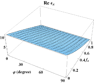
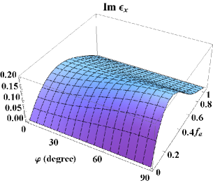
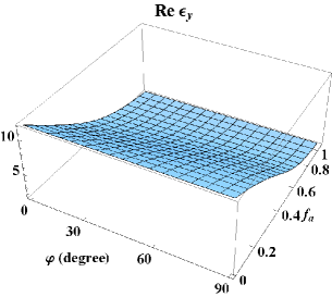
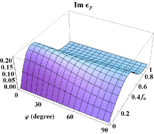
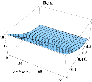
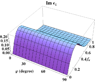
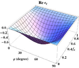
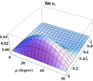
Figure 1: The extended Bruggeman estimates of relative permittivity parameters of the HCM plotted versus volume fraction $f_{a}\in\left(0,1\right)$ and spheroid orientation angle $\varphi\in\left(0^{\circ},90^{\circ}\right)$. The relative size parameter $k_{\scriptscriptstyle 0}\eta=0.2$ and the eccentricity parameter $\rho=9$.

The extended Bruggeman estimates of the HCM’s relative permittivity parameters $\epsilon_{x,y,z,t}$ are plotted as functions of spheroid orientation angle $\varphi$ and volume fraction $f_{a}$ in Fig. 1. Here, we fixed the relative size parameter $\eta=0.2/k_{\scriptscriptstyle 0}$ and the eccentricity parameter $\rho=9$. We see that the real parts of $\epsilon_{x,y,z}$ decay almost linearly as $f_{a}$ increases from 0 to 1, but $\mbox{Re}\left\{\epsilon_{x,y,z}\right\}$ are largely insensitive to variations in $\varphi$. While the real part of $\epsilon_{t}$ is nonexistent for $\varphi=0^{\circ}$ and $90^{\circ}$, and also in the limits $f_{a}\to 0$ and $1$, away from these boundary values we have $\mbox{Re}\left\{\epsilon_{t}\right\}<0$ with a local minimum occurring at approximately $\varphi=45^{\circ}$ and $f_{a}=0.26$. The imaginary parts of $\epsilon_{x,y,z}$ attain their largest values in the vicinity of $f_{a}=0.26$, and vanish at $f_{a}=0$ and 1. As $\varphi$ increases from zero, $\mbox{Im}\left\{\epsilon_{x}\right\}$ generally increases, $\mbox{Im}\left\{\epsilon_{y}\right\}$ generally decreases, and $\mbox{Im}\left\{\epsilon_{z}\right\}$ is largely unchanged. The imaginary part of $\epsilon_{t}$ is null-valued along the boundaries $\varphi=0^{\circ}$ and $90^{\circ}$, and $f_{a}=0$ and $1$, but away from these boundary values $\mbox{Im}\left\{\epsilon_{t}\right\}$ exhibits a local maximum which coincides with the local minimum exhibited by $\mbox{Re}\left\{\epsilon_{t}\right\}$. The following two limits, which hold for arbitrary $f_{a}\in\left(0,1\right)$, are especially noteworthy: (a) As $\varphi\to 0^{\circ}$, we find that $\epsilon_{x}\neq\epsilon_{y}=\epsilon_{z}$; i.e., the HCM is uniaxial. Accordingly the HCM cannot support Voigt wave propagation in this limit [27]. (b) As $\varphi\to 90^{\circ}$, we find that $\epsilon_{x}$, $\epsilon_{y}$ and $\epsilon_{z}$ are all different while $\epsilon_{t}=0$; i.e., the HCM’s biaxial structure is orthorhombic.

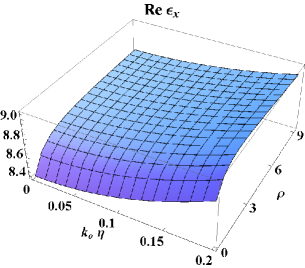
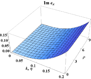
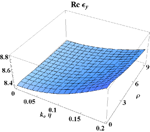
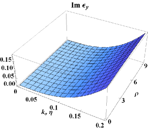
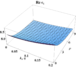
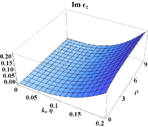
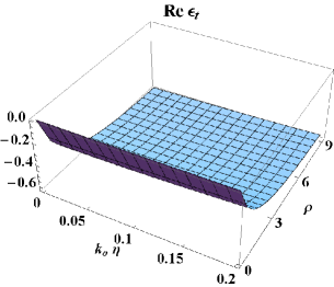
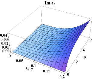
Figure 2: As Fig. 1 except that the HCM’s relative permittivity parameters are plotted versus the relative size parameter $k_{\scriptscriptstyle 0}\eta\in\left(0,0.2\right)$ and the eccentricity parameter $\rho\in\left(0,9\right)$. The volume fraction $f_{a}=0.25$ and spheroid orientation angle $\varphi=45^{\circ}$.

Next we turn to the dependency upon the component particle shape and size. In Fig. 2, $\epsilon_{x,y,z,t}$ are plotted against relative size parameter $k_{\scriptscriptstyle 0}\eta$ and the eccentricity parameter $\rho$. Here, we fixed the volume fraction $f_{a}=0.25$ and the spheroid orientation angle $\varphi=45^{\circ}$. The real parts of $\epsilon_{x,y,z}$ generally increase as $\eta$ increases, whereas $\mbox{Re}\left\{\epsilon_{t}\right\}$ is largely independent of $\eta$. As $\rho$ increases, $\mbox{Re}\left\{\epsilon_{x}\right\}$ generally increases but $\mbox{Re}\left\{\epsilon_{y,z,t}\right\}$ generally decrease. The most conspicuous feature of the plots of $\mbox{Im}\left\{\epsilon_{x,y,z,t}\right\}$ is that these quantities increase uniformly from zero as $\eta$ increases from zero. Also, $\mbox{Im}\left\{\epsilon_{x,y,z}\right\}$ are fairly insensitive to increasing $\rho$ but $\mbox{Im}\left\{\epsilon_{t}\right\}$ increases markedly as $\rho$ increases. Let us note that in the limit $\rho\to 0$, we have $\epsilon_{x}=\epsilon_{y}=\epsilon_{z}$ and $\epsilon_{t}=0$; i.e., the HCM is an isotropic dielectric material, regardless of the size parameter $\eta$ (or the orientation angle $\varphi$ and volume fraction $f_{a}$).

4.3 Orientations for Voigt waves

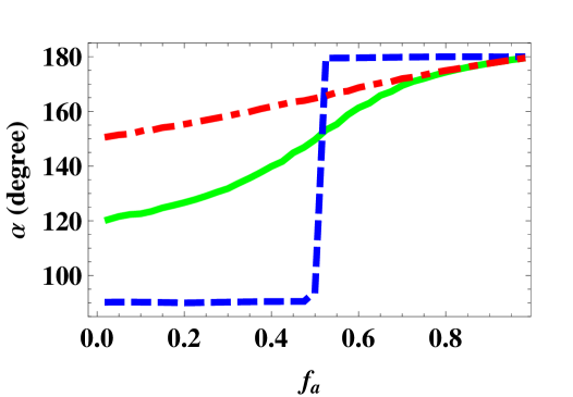
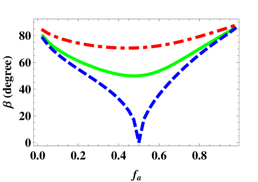
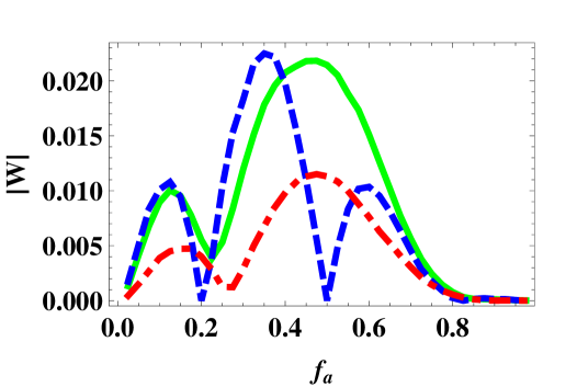
Figure 3: The angular coordinates $\alpha$, $\beta$, and the absolute value of the quantity $W$, plotted versus volume fraction $f_{a}$ for spheroid orientation angle $\varphi=90^{\circ}$ (blue, dashed curves), $60^{\circ}$ (green, solid curves) and $30^{\circ}$ (red, broken dashed curves). The size parameter $\eta=0.2/k_{\scriptscriptstyle 0}$ and the eccentricity parameter $\rho=9$.

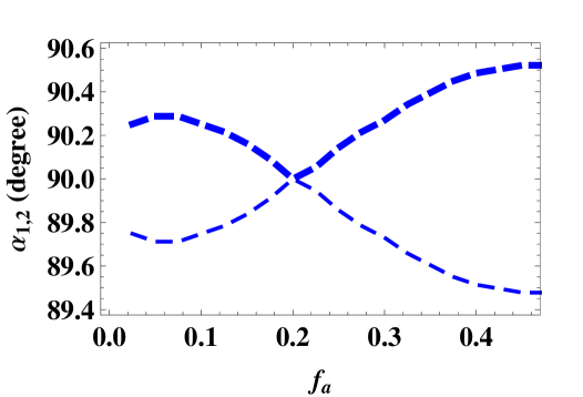
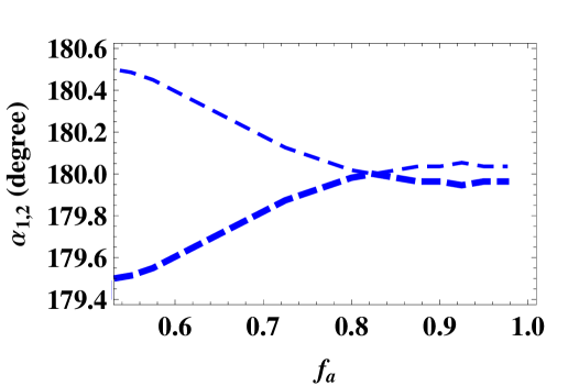
Figure 4: Close-up plots of $\alpha$ versus $f_{a}$ in Fig. 3 for $\varphi=90^{\circ}$.

Before presenting in detail the results of our numerical study of Voigt wave propagation in the HCM characterized in Figs. 1 and 2, the following should be pointed out. In general, for a given HCM the Voigt wave conditions $Y=0$ and $W\neq 0$ are satisfied at two distinct orientations, specified by the angular coordinates $\alpha=\alpha_{1,2}$ and $\beta=\beta_{1,2}$. However, for the numerical investigations reported herein we found that $\alpha_{1}\approx\alpha_{2}$ and $\beta_{1}\approx\beta_{2}$, with the differences between the two orientations being at most approximately $1\%$ and often much less. Consequently, each curve of $\alpha$, corresponding to a zero of $|Y|$, presented in the following Figs. 3, 6 and 7 would appear at higher resolution as two very closely-spaced curves, namely that of $\alpha_{1}$ and that of $\alpha_{2}$. And similarly for each curve of $\beta$, and the corresponding curves of $|W|$, in Figs. 3, 6 and 7. However, at the resolution of Figs. 3, 6 and 7 this is difficult to perceive. This matter is elaborated upon in due course, in the discussion of Figs. 4 and 5.

Let us now begin by considering the effects of volume fraction $f_{a}$, and spheroid orientation angle $\varphi$, on Voigt wave propagation in the HCM characterized in Figs. 1 and 2. The angular coordinates $\alpha$ and $\beta$ of the zeros of $|Y|$, along with the corresponding values of $|W|$, are plotted versus $f_{a}\in\left(0,1\right)$ in Fig. 3 for $\varphi=30^{\circ}$, $60^{\circ}$ and $90^{\circ}$. The $\alpha$ coordinate for $\varphi=90^{\circ}$ changes abruptly at $f_{a}=0.48$, from being very close to $90^{\circ}$ for $f_{a}<0.48$ to being very close to $180^{\circ}$ for $f_{a}>0.48$. The change in the $\alpha$ coordinate for mid-range values of $f_{a}$ becomes progressively less abrupt as $\varphi$ decreases: for $\varphi=60^{\circ}$ the corresponding graph of $\alpha$ is approximately sigmoidal while for $\varphi=30^{\circ}$ the graph is nearly linear. The $\beta$ coordinate is also highly sensitive to the volume fraction. Indeed, for $\varphi=90^{\circ}$, the value of $\beta$ ranges from $0^{\circ}$ at $f_{a}=0.48$ to $90^{\circ}$ in the limits $f_{a}\to 0$ and $1$. This sensitivity becomes less pronounced as $\varphi$ decreases. From the corresponding graphs of $|W|$, we can deduce for which values of $f_{a}$ the HCM supports Voigt wave propagation. In the limits $f_{a}\to 0$ and $1$ we see that $|W|\to 0$ and therefore the HCM cannot support Voigt waves in these limits. There are three further points for $\varphi=90^{\circ}$, namely $f_{a}=0.2$, $0.48$ and $0.83$, at which $|W|=0$ and the HCM cannot support Voigt wave propagation.

As mentioned earlier, each curve in Fig. 3 (and indeed in Figs. 6 and 7) actually represents two closely-spaced but distinct directions for Voigt wave propagation. In order to better appreciate this feature, in Fig. 4 the curves of $\alpha_{1}$ and $\alpha_{2}$ for $\varphi=90^{\circ}$ in Fig. 3 are reproduced at much higher resolution. The corresponding curves of $\beta_{1,2}$ are indistinguishable even at this higher resolution. At values of $f_{a}<0.48$, the graphs of $\alpha_{1}$ and $\alpha_{2}$ are mirror images with respect to reflection about $\alpha_{1,2}=90^{\circ}$, and the same applies to the $\alpha_{1,2}$ curves for $f_{a}>0.48$ but with respect to the symmetry line $\alpha_{1,2}=180^{\circ}$. The differences between the $\alpha_{1}$ and $\alpha_{2}$ curves ranges from approximately $1^{\circ}$ down to $0^{\circ}$. Notice that the $f_{a}$ values at which the difference is $0^{\circ}$, i.e., $f_{a}=0.2$ and $0.83$, correspond to the zeros of $|W|$ observed in Fig. 3.

In order to illustrate the two distinct orientations for Voigt wave propagation for $\varphi\neq 90^{\circ}$, in Fig. 5 a representative example is provided for $\varphi=30^{\circ}$, with $f_{a}=0.3$ and the eccentricity and size parameters being the same as in Fig. 3. Here the normalized values of $|Y|$ are plotted versus the angular coordinates $\alpha\in\left(164.5^{\circ},165.5^{\circ}\right)$ and $\beta\in\left(70.4^{\circ},71.4^{\circ}\right)$. Two $|Y|$ zeros can be seen: one at $\alpha=164.8^{\circ}$, $\beta=70.9^{\circ}$ and the other at $\alpha=165.2^{\circ}$, $\beta=70.9^{\circ}$.

Next the influence of the component particles’ shape on the propagation of Voigt waves is considered. The angular coordinates $\alpha$ and $\beta$ of the zeros of $|Y|$, along with the corresponding values of $|W|$, are plotted as functions of the eccentricity parameter $\rho\in\left(0,9\right)$ in Fig. 6 for the spheroid orientation angle $\varphi\in\left\{30^{\circ},60^{\circ},90^{\circ}\right\}$. The volume fraction was fixed at $f_{a}=0.25$ and the size parameter $\eta=0.2/k_{\scriptscriptstyle 0}$. The values of $\alpha$ for each value of $\varphi$ are quite different, but these values are almost independent of $\rho$. The values of $\beta$ for each value of $\varphi$ are also quite different, but for the values of this angular coordinate decrease gradually as $\rho$ increases. The corresponding values of $|W|$ increase as $\rho$ increases, most rapidly for $\varphi=90^{\circ}$ and least rapidly for $\varphi=30^{\circ}$. Furthermore, $|W|\to 0$ as $\rho\to 0$, regardless of $\varphi$, as would be expected since the HCM becomes an isotropic dielectric material in this limit.

Lastly, we turn to the effect of the component particle size, as accommodated by the extended Bruggeman formalism. In Fig. 7, graphs of the angular coordinates $\alpha$ and $\beta$ at which $|Y|=0$, and the corresponding values of $|W|$, against the relative size parameter $k_{\scriptscriptstyle 0}\eta\in\left(0,0.2\right)$ are displayed for the spheroid orientation angle $\varphi\in\left\{30^{\circ},60^{\circ},90^{\circ}\right\}$. Here the volume fraction $f_{a}=0.25$ and the eccentricity parameter $\rho=9$. While the size parameter $\eta$ has very little influence upon the orientations for Voigt waves, as indicated by the nearly horizontal graphs of $\alpha$ and $\beta$, it does have a profound influence upon whether or not Voigt waves can propagate. Since $|W|\to 0$ as $\eta\to 0$, we infer that the nondissipative HCM — arising from vanishingly-small component particles — does not support Voigt wave propagation. In contrast, for nonzero values of $\eta$ we see that $|W|>0$ and therefore Voigt wave propagation is supported.

5 Closing remarks

Engineered materials, in the form of HCMs, may be conceptualized which support Voigt wave propagation while their component materials do not. The case considered here involved remarkably simple component materials, namely nondissipative isotropic dielectric materials, in contrast to earlier studies on Voigt-wave-supporting HCMs which involved dissipative uniaxial dielectric components [5, 15]. In the present case, the ability of the HCMs to support Voigt waves relied upon the shape, orientation and nonzero size of the component particles, as well as the volume fraction of the component materials. In order to cater for such component materials, an extended version [18] of the well-established Bruggeman homogenization formalism [17, 19] was needed. We note that the homogenization approaches adopted in earlier Voigt wave studies, to wit the Maxwell-Garnett formalism [5] and strong-permittivity-fluctuation theory [15], could not be used here because they cannot accommodate component particles with differing orientations or component particles of nonzero size.

Our numerical investigations revealed that the directions in which Voigt waves may propagate is highly sensitive to the orientation of the component particles and to the volume fraction of the component materials, but less sensitive to the shape of the component particles and less sensitive still to the size of the component particles. Furthermore, whether or not a HCM supports Voigt wave propagation is critically dependent upon the size of the component particles and, in certain cases, upon the volume fraction. For the scenarios considered at here, it was found that, in general, the two directions which support Voigt wave propagation are very close together. This is consequence of the component materials being nondissipative. For dissipative component materials, these two directions can be more widely spaced [15].

This study further emphasizes the role of the micro- and/or nano-structure in determining the macroscopic optical properties of engineered materials, and paves the way for a study of Voigt wave propagation in bianisotropic HCMs, which — courtesy of their enormous parameter space — present greater scope for Voigt waves.

Figure 5: The normalized values of $|Y|$ plotted versus angular coordinates $\alpha\in\left(164.5^{\circ},165.5^{\circ}\right)$ and $\beta\in\left(70.4^{\circ},71.4^{\circ}\right)$ for spheroid orientation angle $\varphi=30^{\circ}$, volume fraction $f_{a}=0.5$, eccentricity parameter $\rho=9$ and size parameter $\eta=0.2/k_{\scriptscriptstyle 0}$.

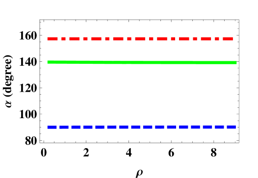
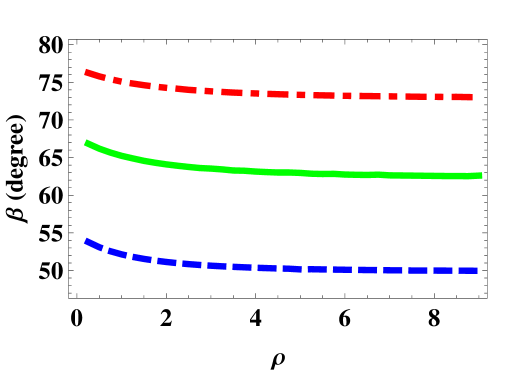
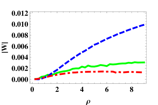
Figure 6: The angular coordinates $\alpha$, $\beta$, and the absolute value of the quantity $W$, plotted versus the eccentricity parameter $\rho$ for spheroid orientation angle $\varphi=90^{\circ}$ (blue, dashed curves), $60^{\circ}$ (green, solid curves) and $30^{\circ}$ (red, broken dashed curves). The size parameter $\eta=0.2/k_{\scriptscriptstyle 0}$ and the volume fraction $f_{a}=0.25$.

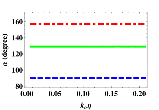
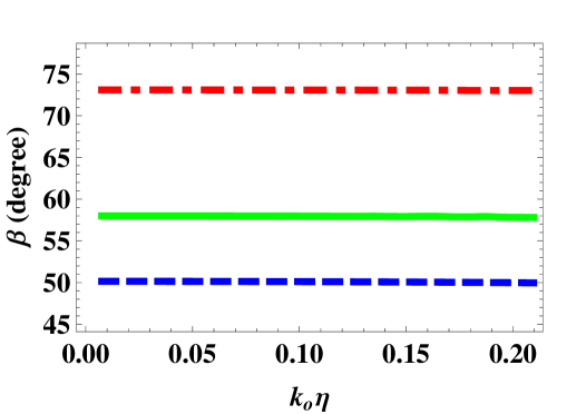
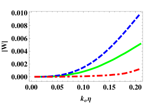
Figure 7: The angular coordinates $\alpha$, $\beta$, and the absolute value of the quantity $W$, plotted versus relative size parameter $k_{\scriptscriptstyle 0}\eta$ for spheroid orientation angle $\varphi=90^{\circ}$ (blue, dashed curves), $60^{\circ}$ (green, solid curves) and $30^{\circ}$ (red, broken dashed curves). The volume fraction $f_{a}=0.25$ and the eccentricity parameter $\rho=9$.

References

- [1] Lakhtakia A (ed) 1996 Selected Papers on Linear Optical Composite Materials (Bellingham WA: SPIE Optical Engineering Press)
- [2] Milton G W 2002 The Theory of Composites (Cambridge, UK: Cambridge University Press)
- [3] Mackay T G and Lakhtakia A 2006 Correlation length and negative phase velocity in isotropic dielectric-magnetic materials J. Appl. Phys. 100 063533
- [4] Mackay T G and Lakhtakia A 2004 Plane waves with negative phase velocity in Faraday chiral mediums Phys. Rev. E 69 026602
- [5] Mackay T G and Lakhtakia A 2003 Voigt wave propagation in biaxial composite materials J. Opt. A: Pure Appl. Opt. 5 91–95
- [6] Born M and Wolf E 1980 Principles of Optics 6th Edition (Oxford, UK: Pergamon Press)
- [7] Voigt W 1902 On the behaviour of pleochroitic crystals along directions in the neighbourhood of an optic axis Phil. Mag. 4 90–97
- [8] Pancharatnam S 1958 The optical interference figures of amethystine quartz — Part II Proc. Ind. Acad. Sci. A 47 210–229
- [9] Khapalyuk A P 1962 On the theory of circular optical axes Opt. Spectrosc. (USSR) 12 52–54
- [10] Fedorov F I and Goncharenko A M 1963 Propgation of light along the circular optical axes of absorbing crystals Opt. Spectrosc. (USSR) 14 51–53
- [11] Agranovich V M and Ginzburg V L 1984 Crystal Optics with Spatial Dispersion, and Excitons (Berlin: Springer)
- [12] Berry M V and Dennis M R 2003 The optical singularities of birefringent dichroic chiral crystals Proc. R. Soc. Lond. A 459 1261–1292
- [13] Berry M V 2005 The optical singularities of bianisotropic crystals Proc. R. Soc. Lond. A 461 2071-2098
- [14] Zhuck N P 1994 Strong–fluctuation theory for a mean electromagnetic field in a statistically homogeneous random medium with arbitrary anisotropy of electrical and statistical properties Phys. Rev. B 50 15636–15645
- [15] Mackay T G and Lakhtakia A 2004 Correlation length facilitates Voigt wave propagation Waves Random Media 14 L1–L11
- [16] Mackay T G and Weiglhofer W S 2000 Homogenization of biaxial composite materials: dissipative anisotropic properties J. Opt. A: Pure Appl. Opt. 2 426–432
- [17] Goncharenko A V 2003 Generalizations of the Bruggeman equation and a concept of shape-distributed particle composites Phys. Rev. E 68 041108
- [18] Mackay T G 2004 Depolarization volume and correlation length in the homogenization of anisotropic dielectric composites Waves Random Media 14 485–498. Erratum: 2006 Waves Random Complex Media 16 85
- [19] Mackay T G and Lakhtakia A 2008 Electromagnetic fields in linear bianisotropic mediums Prog. Opt. 51 121–209
- [20] Mackay T G 2005 Linear and nonlinear homogenized composite mediums as metamaterials Electromagnetics 25 461–481
- [21] Buchanan J L and Turner P R 1992 Numerical Methods and Analysis (New York: McGraw-Hill)
- [22] Michel B 1997 A Fourier space approach to the pointwise singularity of an anisotropic dielectric medium Int. J. Appl. Electromagn. Mech. 8 219–227
- [23] Michel B and Weiglhofer W S 1997 Pointwise singularity of dyadic Green function in a general bianisotropic medium Arch. Elekron. Übertrag. 51 219–223 Erratum 1998 52 31
- [24] Weiglhofer W S 1998 Electromagnetic depolarization dyadics and elliptic integrals J. Phys. A: Math. Gen. 31 7191–7196
- [25] Mackay T G 2008 On extended homogenization formalisms for nanocomposites J. Nanophotonics 2 021850
- [26] Arfken G B and Weber H J 1995 Mathematical Methods for Physicists 4th Edition (London: Academic Press)
- [27] Gerardin J and Lakhtakia A 2001 Conditions for Voigt wave propagation in linear, homogeneous, dielectric mediums Optik 112 493–495
- [28] Van Kranendonk J and Sipe J E 1977 Foundations of the macroscopic electromagnetic theory of dielectric media Prog. Opt. 15 245–350
- [29] Tsang L, Kong J A and Newton R W 1982 Application of strong fluctuation random medium theory to scattering of electromagnetic waves from a half-space of dielectric mixture IEEE Trans. Antennas Propagat. 30 292–302