Bayesian evidence for two companions orbiting HIP 5158

Abstract

We present results of a Bayesian analysis of radial velocity (RV) data for the star HIP 5158, confirming the presence of two companions and also constraining their orbital parameters. Assuming Keplerian orbits, the two-companion model is found to be $e^{48}$ times more probable than the one-planet model, although the orbital parameters of the second companion are only weakly constrained. The derived orbital periods are $345.6\pm 2.0$ d and $9017.8\pm 3180.7$ d respectively, and the corresponding eccentricities are $0.54\pm 0.04$ and $0.14\pm 0.10$. The limits on planetary mass $(m\sin i)$ and semimajor axis are $(1.44\pm 0.14$ $M_{\rm J},0.89\pm 0.01$ AU) and $(15.04\pm 10.55$ $M_{\rm J},7.70\pm 1.88$ AU) respectively. Owing to the large uncertainty on the mass of the second companion, we are unable to determine whether it is a planet or a brown dwarf. The remaining ‘noise’ (stellar jitter) unaccounted for by the model is $2.28\pm 0.31$ m/s. We also analysed a three-companion model, but found it to be $e^{8}$ times less probable than the two-companion model.

1 Introduction

Extrasolar planetary research has made great advances in the last decade as a result of the data gathered by several ground and space based telescopes and so far more than 500 extrasolar planets have been discovered. More and more planets with large orbital periods and small velocity amplitudes are now being detected due to remarkable improvements in the accuracy of RV measurements. With the flood of new data, more powerful statistical techniques are being developed and applied to extract as much information as possible. Traditionally, the orbital parameters of the planets and their uncertainties have been obtained by a two stage process. First the period of the planets is determined by searching for periodicity in the RV data using the Lomb-Scargle periodogram (Lomb 1976; Scargle 1982). Other orbital parameters are then determined using minimisation algorithms, with the orbital period of the planets fixed to the values determined by Lomb-Scargle periodogram.

Bayesian methods have several advantages over traditional methods, for example when the data do not cover a complete orbital phase of the planet. Bayesian inference also provides a rigorous way of performing model selection which is required to decide the number of planets favoured by the data. The main problem in applying such Bayesian model selection techniques is the computational cost involved in calculating the Bayesian evidence. Nonetheless, Bayesian model selection has the potential to improve the interpretation of existing observational data and possibly detect yet undiscovered planets. Recent advances in Marko-Chain Monte Carlo (MCMC) techniques (see e.g. Mackay 2003) have made it possible for Bayesian techniques to be applied to extrasolar planetary searches (see e.g. Gregory 2005; Ford 2005; Ford & Gregory 2007; Balan & Lahav 2009). Feroz et al. (2010) recently presented a new Bayesian method for determining the number of extrasolar planets, as well as for inferring their orbital parameters, without having to calculate directly the Bayesian evidence for models containing a large number of planets, although this method is not required for the analysis of the simple system considered here.

HIP 5158 is a K-type main sequence star at a distance of $45\pm 4$ pc with mass $0.780\pm 0.021$ $M_{\sun}$ (Lo Curto et al., 2010). In this paper, we present a Bayesian analysis of the existing, high-precision RV measurements of HIP 5158 from the HARPS instrument (Mayor et al., 2003), given in Lo Curto et al. (2010), who detected a planet with period $345.72\pm 5.37$ d. They did not find any correlation of the RV with the bispector span of the cross correlation function for HIP 5158. They also did not find any periodicity in the stellar activity indicator $\log R_{\rm HK}^{\prime}$, making it unlikely for any long period RV variability to be caused by stellar activity. Moreover, they noticed an additional quadratic drift in the RV data which they inferred to indicate the presence of another body orbiting the star, but they were not able to constrain its orbital parameters.

The outline of this paper is as follows. We give a brief introduction to Bayesian inference in Sec. 2 and describe our method for calculating the number of planets favoured by the data. Our model for calculating RV is described in Sec. 3. In Sec. 4 we describe our Bayesian analysis methodology. We apply our method to RV data sets on HIP 5158 in Sec. 5 and present our conclusions in Sec. 6.

2 Bayesian inference

Our planet finding methodology is built upon the principles of Bayesian inference, and so we begin by giving a brief summary of this framework. We refer the reader to Feroz et al. (2010) for a more thorough discussion on Bayesian object detection methods.

Bayesian inference methods provide a consistent approach to the estimation of a set of parameters $\mathbf{\Theta}$ in a model (or hypothesis) $H$ for the data $\mathbf{D}$. Bayes’ theorem states that

$$\Pr(\mathbf{\Theta}|\mathbf{D},H)=\frac{\Pr(\mathbf{D}|\,\mathbf{\Theta},H)\Pr(\mathbf{\Theta}|H)}{\Pr(\mathbf{D}|H)},$$ (1)

where $\Pr(\mathbf{\Theta}|\mathbf{D},H)\equiv P(\mathbf{\Theta})$ is the posterior probability distribution of the parameters, $\Pr(\mathbf{D}|\mathbf{\Theta},H)\equiv\mathcal{L}(\mathbf{\Theta})$ is the likelihood, $\Pr(\mathbf{\Theta}|H)\equiv\pi(\mathbf{\Theta})$ is the prior, and $\Pr(\mathbf{D}|H)\equiv\mathcal{Z}$ is the Bayesian evidence.

In parameter estimation, the normalising evidence factor can be ignored, since it is independent of the parameters $\mathbf{\Theta}$, and inferences are obtained by taking samples from the (unnormalised) posterior using standard MCMC methods, where at equilibrium the chain contains a set of samples from the parameter space distributed according to the posterior. This posterior constitutes the complete Bayesian inference of the parameter values, and can be marginalised over each parameter to obtain individual parameter constraints.

In contrast to parameter estimation problems, for model selection the evidence needs to be evaluated and is simply the factor required to normalize the posterior over $\mathbf{\Theta}$:

$$\mathcal{Z}=\int{\mathcal{L}(\mathbf{\Theta})\pi(\mathbf{\Theta})}d^{D}\mathbf{\Theta},$$ (2)

where $D$ is the dimensionality of the parameter space. As the average of the likelihood over the prior, the evidence is larger for a model if more of its parameter space is likely and smaller for a model with large areas in its parameter space having low likelihood values, even if the likelihood function is very highly peaked. Thus, the evidence automatically implements Occam’s razor: a simpler theory with compact parameter space will have a larger evidence than a more complicated one, unless the latter is significantly better at explaining the data. The question of model selection between two models $H_{0}$ and $H_{1}$ can then be decided by comparing their respective posterior probabilities given the observed data set $\mathbf{D}$, as follows

$$R=\frac{\Pr(H_{1}|\mathbf{D})}{\Pr(H_{0}|\mathbf{D})}=\frac{\Pr(\mathbf{D}|H_{1})\Pr(H_{1})}{\Pr(\mathbf{D}|H_{0})\Pr(H_{0})}=\frac{\mathcal{Z}_{1}}{\mathcal{Z}_{0}}\frac{\Pr(H_{1})}{\Pr(H_{0})},$$ (3)

where $\Pr(H_{1})/\Pr(H_{0})$ is the a priori probability ratio for the two models, which can often be set to unity but occasionally requires further consideration. The natural logarithm of the ratio of posterior model probabilities (sometimes termed the posterior odds ratio) provides a useful guide to what constitutes a significant difference between two models:

$$\Delta\ln R=\ln\left[\frac{\Pr(H_{1}|\mathbf{D})}{\Pr(H_{0}|\mathbf{D})}\right]=\ln\left[\frac{\mathcal{Z}_{1}}{\mathcal{Z}_{0}}\frac{\Pr(H_{1})}{\Pr(H_{0})}\right].$$ (4)

The evaluation of the number of objects favoured by the data is a model selection problem. By considering a series of models $H_{N_{\rm obj}}$, each with a fixed number of objects, i.e. with $N_{\rm obj}=0,1,2,\ldots$, one can infer $N_{\rm obs}$ by identifying the model with the largest marginal posterior probability $\Pr(H_{N_{\rm obj}}|\mathbf{D})$. The probability associated with $N_{\rm obj}=0$ is often called the ‘null evidence’ and provides a baseline for comparison of different models. Indeed, this approach has been adopted previously in exoplanet studies (see e.g. Gregory & Fischer (2010)), albeit using only lower-bound estimates of the Bayesian evidence for each model.

Evaluation of the multidimensional integral in Eq. 2 is a challenging numerical task. Standard techniques like thermodynamic integration are extremely computationally expensive which makes evidence evaluation at least an order of magnitude more costly than parameter estimation. The nested sampling approach, introduced by Skilling (2004), is a Monte Carlo method targeted at the efficient calculation of the evidence, but also produces posterior inferences as a by-product. Feroz & Hobson (2008) and Feroz et al. (2009b) built on this nested sampling framework and have recently introduced the MultiNest algorithm which is very efficient in sampling from posteriors that may contain multiple modes and/or large (curving) degeneracies and also calculates the evidence. This technique has greatly reduces the computational cost of Bayesian parameter estimation and model selection and has already been applied to several model selections problem in astrophysics (see e.g. Feroz et al. 2008; Feroz et al. 2009c; Feroz et al. 2009a). We employ this technique in this paper.

3 Modelling Radial Velocities

Observing planets at interstellar distances directly is extremely difficult, since the planets only reflect the light incident on them from their host star and are consequently many times fainter. Nonetheless, the gravitational force between the planets and their host star results in the planets and star revolving around their common centre of mass. This produces doppler shifts in the spectrum of the host star according to its RV, the velocity along the line-of-sight to the observer. Several such measurements, usually over an extended period of time, can then be used to detect extrasolar planets.

Following the formalism given in Balan & Lahav (2009), for $N_{\rm p}$ planets and ignoring the planet-planet interactions, the RV at an instant $t_{\rm i}$ observed at $j$th observatory can be calculated as:

$$v(t_{\rm i},j)=V_{\rm j}-\sum_{\rm p=1}^{N_{\rm p}}K_{\rm p}\left[\sin(f_{\rm i,p}+\varpi_{\rm p})+e_{\rm p}\sin(\varpi_{\rm p})\right],$$ (5)

where

$$V_{\rm j} = \mbox{systematic velocity with reference to $j$th observatory},$$

$$K_{\rm p} = \mbox{velocity semi-amplitude of the $p$th planet},$$

$$\varpi_{\rm p} = \mbox{longitude of periastron of the $p$th planet},$$

$$f_{\rm i,p} = \mbox{true anomaly of the $p$th planet},$$

$$e_{\rm p} = \mbox{orbital eccentricity of the $p$th planet},$$

start of data taking, at which periastron occurred.

Note that $f_{\rm i,p}$ is itself a function of $e_{\rm p}$, the orbital period $P_{\rm p}$ of the $p$th planet, and the fraction $\chi_{\rm p}$ of an orbit of the $p$th planet, prior to the start of data taking, at which periastron occurred. While there is a unique mean line-of-sight velocity of the center of motion, it is important to have a different velocity reference $V_{\rm j}$ for each observatory/spectrograph pair, since the velocities are measured differentially relative to a reference frame specific to each observatory.

Parameter	Prior	Mathematical Form	Lower Bound	Upper Bound
$P$ (days)	Jeffreys	$\frac{1}{P\ln(P_{\rm max}/P_{\rm min})}$	$0.2$	$365,000$
$K$ (m/s)	Mod. Jeffreys	$\frac{(K+K_{0})^{-1}}{\ln(1+(K_{\rm max}/K_{0})(P_{\rm min}/P_{\rm i})^{1/3}(1/\sqrt{1-e_{\rm i}^{2}}))}$	$0$	$K_{\rm max}(P_{\rm min}/P_{\rm i})^{1/3}(1/\sqrt{1-e_{\rm i}^{2}})$
$V$ (m/s)	Uniform	$\frac{1}{V_{\rm min}-V_{\rm max}}$	$-K_{\rm max}$	$K_{\rm max}$
$e$	Uniform	$1$	$0$	$1$
$\varpi$ (rad)	Uniform	$\frac{1}{2\pi}$	$0$	$2\pi$
$\chi$	Uniform	$1$	$0$	$1$
$s$ (m/s)	Mod. Jeffreys	$\frac{(s+s_{0})^{-1}}{\ln(1+s_{\rm max}/s_{0})}$	$0$	$K_{\rm max}$

Table 1: Prior probability distributions.

We also model the intrinsic stellar variability $s$ (‘jitter’), as a source of uncorrelated Gaussian noise in addition to the measurement uncertainties. Therefore for each planet we have five free parameters: $K$, $\varpi$, $e$, $P$ and $\chi$. In addition to these parameters there are two nuisance parameters $V$ and $s$, common to all the planets.

These orbital parameters can then be used along with the stellar mass $m_{\rm s}$ to calculate the length $a$ of the semi-major axis of the planet’s orbit around the centre of mass and the planetary mass $m$ as follows:

$$a_{\rm s}\sin i = \frac{KP\sqrt{1-e^{2}}}{2\pi},$$ (6)

$$m\sin i \approx \frac{Km_{\rm s}^{\frac{2}{3}}P^{\frac{1}{3}}\sqrt{1-e^{2}}}{(2\pi G)^{\frac{1}{3}}},$$ (7)

$$a \approx \frac{m_{\rm s}a_{\rm s}\sin i}{m\sin i},$$ (8)

where $a_{\rm s}$ is the semi-major axis of the stellar orbit about the centre-of-mass and $i$ is the angle between the direction normal to the planet’s orbital plane and the observer’s line of sight. Since $i$ cannot be measured with RV data, only a lower bound on the planetary mass $m$ can be estimated.

4 Bayesian Analysis of Radial Velocity Measurements

There are several RV search programmes looking for extrasolar planets. The RV measurements consist of the time $t_{\rm i}$ of the $i$th observation, the measured RV $v_{\rm i}$ relative to a reference frame and the corresponding measurement uncertainty $\sigma_{\rm i}$. These RV measurements can be analysed using Bayes’ theorem given in Eq. 1 to obtain the posterior probability distributions of the model parameters discussed in the previous section. We now describe the form of the likelihood and prior probability distributions.

4.1 Likelihood function

As discussed in Gregory (2007), the errors on RV measurements can be treated as Gaussian and therefore the likelihood function can be written as:

$$\mathcal{L}(\Theta)=\prod_{\rm i}\frac{1}{\sqrt{2\pi(\sigma_{\rm i}^{2}+s^{2})}}\exp\left[-\frac{(v(\Theta;t_{\rm i})-v_{\rm i})^{2}}{2(\sigma_{\rm i}^{2}+s^{2})}\right],$$ (9)

where $v_{\rm i}$ and $\sigma_{\rm i}$ are the $i^{\rm th}$ RV measurement and its corresponding uncertainty respectively, $v(\Theta;t_{\rm i})$ is the predicted RV for the set of parameters $\Theta$, and $s$ is intrinsic stellar variability. A large value of $s$ can also indicate the presence of additional planets, e.g. if a two-planet system is analysed with a single-planet model then the velocity variations introduced by the second planet would act like an additional noise term and therefore contribute to $s$.

4.2 Choice of priors

For parameter estimation, priors become largely irrelevant once the data are sufficiently constraining, but for model selection the prior dependence always remains. Therefore, it is important that priors are selected based on physical considerations. We follow the choice of priors given in Gregory (2007), as shown in Table 1.

The modified Jeffreys prior,

$$\Pr(\theta|H)=\frac{1}{(\theta+\theta_{0})\ln(1+\theta_{\rm max}/\theta_{0})},$$ (10)

behaves like a uniform prior for $\theta\ll\theta_{0}$ and like a Jeffreys prior (uniform in $\log$) for $\theta\gg\theta_{0}$. We set $K_{0}=s_{0}=1$ m/s and $K_{\rm max}=2129$ m/s, which corresponds to a maximum planet-star mass ratio of $0.01$.

5 Results

$N_{\rm p}$	$\ln\mathcal{Z}$	$s$ (m/s)
$1$	$30.05\pm 0.14$	$10.31\pm 1.09$
$2$	$78.19\pm 0.15$	$2.28\pm 0.31$
$3$	$70.68\pm 0.16$	$2.28\pm 0.28$

Table 2: The evidence and jitter values for the system HIP 5158. The null evidence ($-255.3$) has been subtracted from each $\ln\mathcal{Z}$ value.

As discussed in Sec. 2, the number of companions orbiting a star can be determined by analysing the RV data, starting with $N_{\rm p}=0$ and increasing it until the Bayesian evidence for $N_{\rm p}=n$ companions starts to drop off. The resulting evidence and jitter values for HIP 5158 RV data, after subtracting a mean RV of $14.9105$ km/s from it, are presented in Table 2. We can clearly see $N_{\rm p}=2$ is the strongly favoured model. Adopting the 2-companion model, the estimated parameter values are listed in Table 3 while the 1-D marginalised posterior probability distributions are shown in Fig. 1. As mentioned in Sec. 1, stellar activity is unlikely to be the source of any long period RV variability of HIP 5158. Moreover, the inferred period of HIP 5158 c is more than two orders of magnitude higher than the rotation period of the star ($P_{\rm rot}(\log R_{\rm HK}^{\prime})=42.3$ d, Lo Curto et al. 2010). We therefore conclude that it is unlikely for the second signal to be generated by the photospheric activity of HIP 5158.

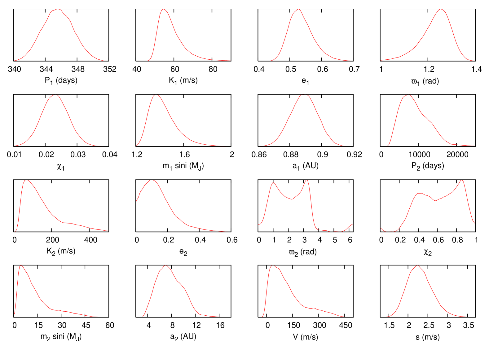
Figure 1: 1-D marginalised posterior probability distributions for the parameters of the two bodies found orbiting HIP 5158.

The mean RV curve for 1 and 2-companion models are overlaid on the RV measurements in Fig. 2. The RV residuals after fitting for 1 and 2 companions along with nuisance parameters (constant systematic velocity and stellar jitter) are shown in Fig. 3, and are obtained by subtracting the estimated mean RV from the measured RV and adding the estimated stellar jitter in quadrature to the quoted RV uncertainties. The 1-companion fit is clearly very poor due to the presence of quadratic drift in the RV data, whereas the residuals from the 2-companion fit are consistent with a noise-only model. Fig. 4 shows histograms of normalised data residuals, defined as follows:

$$v_{\rm r,i}=\frac{v_{\rm i}-\bar{v}_{\rm i}}{\sqrt{\sigma_{\rm i}^{2}+\bar{s}^{2}}},$$ (11)

where $v_{\rm i}$, $\sigma_{\rm i}$ and $\bar{v}_{\rm i}$ are the measured RV, measured RV uncertainty and the estimated mean RV respectively, all at time $t_{\rm i}$ and $\bar{s}$ is the estimated mean stellar jitter. The histogram for the normalised residuals in the 1-companion fit (left panel) has a similar width to the corresponding histogram for the 2-companion fit (right panel), but it should be noted that $\bar{s}$ appearing in the normalisation of Eq. 11 is much smaller in the latter case (see Table 2)

Parameter	HIP 5158 b	HIP 5158 c
$P$ (days)	$345.63\pm 1.99$	$9017.76\pm 3180.74$
	$(341.82,349.53)$	$(3567.13,18193.94)$
	$(344.74)$	$(11135.63)$
$K$ (m/s)	$59.05\pm 7.73$	$170.54\pm 110.17$
	$(49.89,77.47)$	$(36.59,416.85)$
	$(56.65)$	$(218.49)$
$e$	$0.54\pm 0.04$	$0.14\pm 0.10$
	$(0.47,0.63)$	$(0.01,0.40)$
	$(0.54)$	$(0.00)$
$\varpi$ (rad)	$1.23\pm 0.07$	$2.48\pm 1.32$
	$(1.06,1.34)$	$(0.33,5.90)$
	$(1.24)$	$(2.23)$
$\chi$	$0.02\pm 0.00$	$0.57\pm 0.23$
	$(0.02,0.02)$	$(0.12,0.95)$
	$(0.02)$	$(0.59)$
$m\sin i$ ($M_{\rm J}$)	$1.44\pm 0.14$	$15.04\pm 10.55$
	$(1.26,1.77)$	$(2.34,41.49)$
	$(1.34)$	$(19.53)$
$a$ (AU)	$0.89\pm 0.01$	$7.70\pm 1.88$
	$(0.87,0.91)$	$(4.22,12.50)$
	$(0.87)$	$(8.83)$

Table 3: Estimated parameter values for the two bodies found orbiting HIP 5158. The estimated values in the first row are quoted as $\mu\pm\sigma$ where $\mu$ and $\sigma$ are the posterior mean and standard deviation respectively. The interval in the second row is the $95\%$ confidence interval and the number in parenthesis in the third row is the maximum-likelihood parameter value.

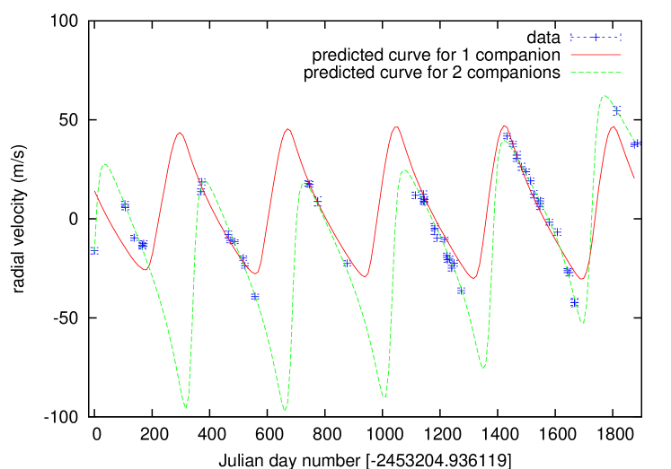
Figure 2: RV measurements, with $1\sigma$ errorbars, and the mean fitted RV curve with 1 (red solid line) and 2-companions (green dashed line) for HIP 5158.

Figure 3: RV residuals, with $1\sigma$ errorbars that include the estimated stellar jitter, after fitting for one (red solid bars) and two companions (blue dotted bars).

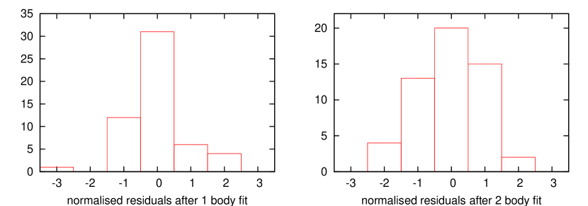
Figure 4: Histograms of normalised RV residuals, as defined in Eq. 11.

Comparing our parameter values with those given in Lo Curto et al. (2010), we see that our parameter estimates for planet HIP 5158 b are in very good agreement. The large uncertainties on the parameter estimates of HIP 5158 c are because not enough phase has been covered by the RV measurements. Nevertheless, we can still determine that the period of the second companion is greater than 10 years with the $95\%$ confidence interval being $(3567,18194)$ days. The corresponding $95\%$ confidence intervals for minimum mass and semi-major axis of the second companion are $(2.3,41.5)$ $M_{\rm J}$ and $(4.2,12.5)$ AU respectively and therefore we can not determine whether it is a planet or a brown dwarf.

6 Conclusions

We have presented a Bayesian analysis of HIP 5158 RV data. Using Bayesian model selection, we have found a very strong signal for the presence of two companions orbiting HIP 5158. Our estimated orbital parameters for the planet HIP 5158 b are in excellent agreement with the values given in Lo Curto et al. (2010). We determined the orbital period of HIP 5158 c to be at least 10 years but the presence of large uncertainties in its orbital parameters do not allow us to determine whether it is a planet or a brown dwarf.

References

- Balan & Lahav (2009) Balan S. T., Lahav O., 2009, MNRAS, 394, 1936
- Feroz et al. (2010) Feroz F., Balan S. T., Hobson M. P., 2010, arXiv e-prints [arXiv:1012.5129]
- Feroz et al. (2009a) Feroz F., Gair J. R., Hobson M. P., Porter E. K., 2009a, Classical and Quantum Gravity, 26, 215003
- Feroz & Hobson (2008) Feroz F., Hobson M. P., 2008, MNRAS, 384, 449
- Feroz et al. (2009b) Feroz F., Hobson M. P., Bridges M., 2009b, MNRAS, 398, 1601
- Feroz et al. (2009c) Feroz F., Hobson M. P., Zwart J. T. L., Saunders R. D. E., Grainge K. J. B., 2009c, MNRAS, 398, 2049
- Feroz et al. (2008) Feroz F., Marshall P. J., Hobson M. P., 2008, arXiv e-prints [arXiv:0810.0781]
- Ford (2005) Ford E. B., 2005, AJ, 129, 1706
- Ford & Gregory (2007) Ford E. B., Gregory P. C., 2007, in G. J. Babu & E. D. Feigelson ed., Statistical Challenges in Modern Astronomy IV Vol. 371 of Astronomical Society of the Pacific Conference Series, Bayesian Model Selection and Extrasolar Planet Detection. pp 189–+
- Gregory (2005) Gregory P. C., 2005, ApJ, 631, 1198
- Gregory (2007) Gregory P. C., 2007, MNRAS, 374, 1321
- Gregory & Fischer (2010) Gregory P. C., Fischer D. A., 2010, MNRAS, 403, 731
- Lo Curto et al. (2010) Lo Curto G., Mayor M., Benz W., Bouchy F., Lovis C., Moutou C., Naef D., Pepe F., Queloz D., Santos N. C., Segransan D., Udry S., 2010, A&A, 512, A48+
- Lomb (1976) Lomb N. R., 1976, Ap&SS, 39, 447
- Mackay (2003) Mackay D. J. C., 2003, Information Theory, Inference and Learning Algorithms. Cambridge University Press, Cambridge, UK
- Mayor et al. (2003) Mayor et al., 2003, The Messenger, 114, 20
- Scargle (1982) Scargle J. D., 1982, ApJ, 263, 835
- Skilling (2004) Skilling J., 2004, in Fischer R., Preuss R., Toussaint U. V., eds, American Institute of Physics Conference Series Nested Sampling. pp 395–405