Analysis of a Darcy-Cahn-Hilliard Diffuse Interface Model for the Hele-Shaw Flow and its Fully Discrete Finite Element Approximation

Abstract

In this paper we present PDE and finite element analyses for a system of partial differential equations (PDEs) consisting of the Darcy equation and the Cahn-Hilliard equation, which arises as a diffuse interface model for the two phase Hele-Shaw flow. In the model the two sets of equations are coupled through an extra phase induced force term in the Darcy equations and a fluid induced transport term in the Cahn-Hilliard equation. We propose a fully discrete implicit finite element method for approximating the PDE system, which consists of the implicit Euler method combined with a convex splitting energy strategy for the temporal discretization, the standard finite element discretization for the pressure and a split (or mixed) finite element discretization for the fourth order Cahn-Hilliard equation. It is shown that the proposed numerical method satisfies a mass conservation law in addition to a discrete energy law that mimics the basic energy law for the Darcy-Cahn-Hilliard phase field model and holds uniformly in the phase field parameter $\varepsilon$. With help of the discrete energy law, we first prove that the fully discrete finite method is unconditionally energy stable and uniquely solvable at each time step. We then show that, using the compactness method, the finite element solution has an accumulation point that is a weak solution of the PDE system. As a result, the convergence result also provides a constructive proof of the existence of global-in-time weak solutions to the Darcy-Cahn-Hilliard phase field model in both two and three dimensions. Finally, we propose a nonlinear multigrid iterative algorithm to solve the finite element equations at each time step. Numerical experiments based on the overall solution method of combining the proposed finite element discretization and a nonlinear multigrid solver are presented to validate the theoretical results and to show the effectiveness of the proposed fully discrete finite element method for approximating the Darcy-Cahn-Hilliard phase field model.

1 Introduction

Hele-Shaw flow refers to the motion of (one or more) viscous fluids between two flat parallel plates separated by an infinitesimally small gap. Such a physical setup is often called a Hele-Shaw cell and was originally designed by Hele-Shaw to study two dimensional potential flows [17]. Various fluid mechanics problems can be approximated by Hele-Shaw flows and thus the research of those flows is of great practical importance. In addition, the relative simplicity of the governing equations of these flows makes Hele-Shaw flows ideal test cases in which rigorous mathematical theory and efficient numerical methods can be developed for studying interfacial dynamics — such as the formation of singularities and topological changes — in immiscible fluids (cf. [20, 21, 24] and the references therein).

The governing equation of Hele-Shaw flow is identical to that of the inviscid potential flow and to the flow of fluids through a porous medium, because the gap-averaged velocity of the fluid is given by Darcy’s law. Specifically, the two phase Hele-Shaw flow takes the form (cf. [20] and the references therein):

(1) $$\mathbf{u} =-\frac{1}{12\eta}\bigl{(}\nabla p-\rho\mathbf{g}\bigr{)}, \quad{\mbox{div }}\mathbf{u} =0 \qquad\mbox{in }\Omega_{T}\setminus\Gamma_{t},$$

(2) $$[p] =\gamma\kappa, \quad[\mathbf{u}\cdot\mathbf{n}] =0 \qquad\mbox{on }\Gamma_{t},$$

with a given set of initial and boundary conditions. Here $\Omega_{T}=\Omega\times(0,T)$, where $\Omega\subset\mathbb{R}^{2}$ is a bounded domain. $\Gamma_{t}$ denotes the interface between the fluids at the time $t$ with the normal $\mathbf{n}$. $\mathbf{u}$ is the fluid velocity and $p$ stands for the pressure of the fluids. The symbol $[p]$ stands for the jump of $p$ across the interface $\Gamma_{t}$. $\eta$ is the viscosity, which may have different (positive constant) values on both sides of $\Gamma_{t}$. ${\bf g}$ is the gravitational force per unit mass; and $\rho$ is the mass density of the fluid, which again can take different (positive constant) values on both sides of the interface. Equation (1)a is Darcy’s law [4], and (1)b implies that the fluids are incompressible. Equations (2)a and (2)b are the boundary conditions at the fluid-fluid interface, which represent the mathematical descriptions of the balance of the surface tension forces and the balance of mass, respectively. Equation (2)a is called the Laplace-Young condition, where $\gamma$ is the dimensionless surface tension coefficient and $\kappa$ is the (mean) curvature of the interface $\Gamma_{t}$. Notice that the tangential component of the velocity $\mathbf{u}$ may experience a jump across the interface [20].

Computationally, the above moving interface problem is difficult to solve directly due to the existence of the surface tension on the interface. In addition, during the evolution the fluid interface may experience topological changes such as self-intersection, pinch-off, splitting, and fattening. When that happens, the classical solution of the moving interface problem ceases to exist. In such cases it is very delicate matter to develop a proper notion of generalized solutions, and it becomes even more challenging to compute the generalized solutions when they can be defined.

To overcome the difficulties, an alternative approach for solving moving interface problems is the diffuse interface theory, which was originally developed as methodology for modeling and approximating solid-liquid phase transitions in which the effects of surface tension and non-equilibrium thermodynamic behavior may be important at the interface. In the theory, the interface is represented as a thin layer of finite thickness, as opposed to a sharp interface. Such an idea dates to Poisson, Gibbs, Rayleigh, van der Waals, and Korteweg (see [23, 20] and the references therein). The approach then uses an auxiliary function (called the phase field function) to indicate the “phase”. The phase field function, denoted by $\varphi$ below, assumes distinct values in the bulk phases away from the interfacial region, through which the phase function varies smoothly. The interface itself can be associated with an intermediate contour/level set of the phase function (cf. [2, 3, 8, 22, 23] and the references therein). Generally speaking, the diffuse interface models are expected to converge to some corresponding sharp interface models as the width of the interfacial layer tends to zero.

The diffuse interface model for Hele-Shaw flows to be studied in this paper is given as follows:

(3) $$\mathbf{u} =-\nabla p-\gamma\varphi\nabla\mu \quad\mbox{in }\Omega_{T},$$

(4) $${\mbox{div }}\mathbf{u} =0 \quad\mbox{in }\Omega_{T},$$

(5) $$\varphi_{t}+\mathbf{u}\cdot\nabla\varphi-\varepsilon\Delta\mu =0 \quad\mbox{in }\Omega_{T},$$

(6) $$\mu =-\varepsilon\Delta\varphi+\frac{1}{\varepsilon}f(\varphi) \quad\mbox{in }\Omega_{T},$$

where $f(\varphi)=F^{\prime}(\varphi)$ and $F(\varphi)=\frac{1}{4}(\varphi^{2}-1)^{2}$ is the so-called double-well (potential) energy density, and $0<\varepsilon<1$ is a fixed constant. To close the system, we impose the following initial and boundary conditions

(7) $$\frac{{\partial}p}{{\partial}\mathbf{n}}=\frac{{\partial}\mu}{{\partial}\mathbf{n}}=\frac{{\partial}\varphi}{{\partial}\mathbf{n}} =0 \qquad\mbox{on}\quad{\partial}\Omega_{T}:={\partial}\Omega\times(0,T],$$

(8) $$\varphi(\,\cdot\,,0) =\varphi_{0}^{\varepsilon}(\,\cdot\,) \qquad\mbox{in}\quad\Omega.$$

Note that we have suppressed the superscript $\varepsilon$ in $(\mathbf{u}^{\varepsilon},p^{\varepsilon},\varphi^{\varepsilon})$ for the sake of notational simplicity. Although $\Omega$ is a two-dimensional domain in the original Hele-Shaw problem, in this paper we consider $\Omega\subset\mathbb{R}^{d}$ $(d=2,3)$ because the three-dimensional problem also has a mathematical interest and arises from biological applications [28]. Here the vector $\mathbf{u}(x,t)\in\mathbb{R}^{d}$ and the scalar $p(x,t)\in\mathbb{R}$ denote the velocity and the pressure of the fluid mixture at the space-time point $(x,t)$, respectively. The variables $\varphi(x,t),\,\mu(x,t)\in\mathbb{R}$ are the phase field function and the chemical potential, respectively. $\varphi$ assumes distinct values — namely, $\pm 1$ based on our choice of $F(\varphi)$ — in the bulk phases away from a thin layer of width $O(\varepsilon)$. This thin layer is called the diffuse interface region. It is natural to define the zero level curve of $\varphi$, $\Gamma_{\varepsilon}(t)=\left\{x\in\mathbb{R}^{d}\,\middle|\,\varphi(x,t)=0\right\}$, as the $d-1$ dimensional interface. Eq. (3) with $\gamma=0$ is the Darcy equation [4]. (5) and (6) without the convection term $\mathbf{u}\cdot\nabla\varphi$ is the Cahn-Hilliard equation [8, 11, 23]. Note that if $\gamma=0$, the velocity vanishes, and the Cahn-Hilliard equation results.

The system (3)–(8) is a special case of the BHSCH (Boussinesq-Hele-Shaw-Cahn-Hilliard) model proposed by Lee, Lowengrub, and Goodman in [20]. They showed, using formal asymptotics, that solutions of the BHSCH system converge to those of the Hele-Shaw model (1)–(2) as their interfacial parameter converges to zero. We note that the pressure $p$ in (3) has a different scaling from that in the BHSCH model in [20]. To obtain a similarly scaled pressure, one can simply introduce a redefined pressure in our model via $\tilde{p}=p+\gamma\varphi\mu$. We shall refer (3)–(8) as the DCH (Darcy-Cahn-Hilliard) model/system herein.

Define the Cahn-Hilliard energy functional

(9) $${\mathcal{J}}_{\varepsilon}(\varphi):=\int_{\Omega}\Bigl{[}\frac{\varepsilon}{2}|\nabla\varphi|^{2}+\frac{1}{\varepsilon}F(\varphi)\Bigr{]}\,dx.$$

Like many diffuse interface models (cf. [2, 12, 22, 20, 23]), the DCH system is also a dissipative system as it satisfies the following energy dissipation law (see Sec. 2 for the details):

(10) $$\frac{d{\mathcal{J}}_{\varepsilon}(\varphi)}{dt}+\varepsilon\left\|\nabla\mu\right\|_{L^{2}}^{2}+\frac{1}{\gamma}\left\|\mathbf{u}\right\|_{L^{2}}^{2}=0.$$

As expected, the above energy law plays a vital role in the analysis of the DCH system and in the design and analysis of numerical methods for the system (see Secs. 2–4 for the details).

This paper consists of four additional sections. Section 2 is devoted to the PDE analysis of the initial-boundary value problem (3)–(8). Weak solutions are defined and the uniqueness and regularities of weak solutions are established. Section 3 contains the formulation of our fully discrete implicit finite element method for problem (3)–(8). It is shown that the proposed numerical method satisfies a mass conservation law in addition to a discrete energy law that mimics the basic energy law for the Darcy-Cahn-Hilliard phase field model and holds uniformly in the phase field parameter $\varepsilon$. With help of the discrete energy law, it also proved that the fully discrete finite method is unconditionally energy stable and uniquely solvable at each time step. Section 4 presents a convergence analysis for the proposed fully discrete finite element method. Using the compactness method it is shown that the finite element solution has an accumulation point that is a weak solution of problem (3)–(8). As a byproduct, this convergence result also provides a constructive proof of the existence global-in-time weak solutions to the PDE system (3)–(8) in both two and three dimensions. Finally, in Sec. 5 we provide some results of numerical experiments validating our theoretical results and showing the effectiveness of the proposed fully discrete finite element method. To solve the nonlinear finite element equations at each time step, we propose a nonlinear multigrid iterative method to do the job. The details of the nonlinear multigrid solver and some other algorithmic and implementation issues are described in Appendix A.

2 PDE analysis

The standard space notations are used in this paper, we refer to [1, 9] for their exact definitions. In particular, $B^{*}$ denotes the dual space of a Banach space $B$, and $\mathbf{B}$ denotes the vector Banach space $B^{d}$, where $d$ is the dimension space. Here we shall assume $d=2$ or 3. The symbol $(\cdot,\cdot)$ is used to denote the standard $L^{2}(\Omega)$ inner product, $\left\langle\cdot,\cdot\right\rangle$ stands for the dual product between $H^{1}(\Omega)$ and $(H^{1}(\Omega))^{*}$. $L^{2}_{0}(\Omega)$ denotes the subspace of $L^{2}(\Omega)$ whose functions have zero mean. Throughout the paper, unless stated otherwise, $c$ and $C$ will be used to denote generic positive constants which are independent of $p$, $\mu$, $\varphi$, $\mathbf{u}$, and $\varepsilon$. If, for example, there is a dependence on $\varepsilon$, we shall explicitly write $C=C(\varepsilon)$. As indicated earlier, we shall assume that $0<\varepsilon<1$.

In the next section we shall construct a finite element method which directly approximates variables $p$, $\mu$, and $\varphi$, but not $\mathbf{u}$, which will be computed as an auxiliary variable as needed. Specifically, we shall approximate the pressure equation by a standard finite element method and the phase equation by a mixed finite element method. We remark that it is also a viable strategy that approximates both the pressure equation and the phase equation by mixed finite element methods, which we shall study in a separate work.

To get the governing equations without using $\mathbf{u}$, substituting the expression of $\mathbf{u}$ in (3) into (4) and (5) we get

(11) $${\mbox{div }}\left(\nabla p+\gamma\varphi\nabla\mu\right) =0 \qquad\mbox{in }\Omega_{T},$$

(12) $$\varphi_{t}-\varepsilon\Delta\mu-{\mbox{div }}\left(\varphi\bigl{[}\nabla p+\gamma\varphi\nabla\mu\bigr{]}\right) =0 \qquad\mbox{in }\Omega_{T}.$$

Then the PDE system to be studied and approximated in this paper consists of equations (11), (12), and (6), which are complimented with the boundary and initial conditions (7)–(8).

Motivated by the energy law (10), we define the following weak formulation and solutions to the initial-boundary value problem.

Definition 1.

Let $\varphi_{0}^{\varepsilon}\in H^{1}(\Omega)$. A triple $(p,\mu,\varphi)$ is called a weak solution of problem (11), (12), and (6)–(8) if it satisfies

(13) $$p \in L^{\frac{4}{3}}\left((0,T);H^{1}(\Omega)\cap L^{2}_{0}(\Omega)\right),$$

(14) $$\mu \in L^{2}\bigl{(}(0,T);H^{1}(\Omega)\bigr{)},$$

(15) $$\nabla p+\gamma\varphi\nabla\mu \in L^{2}\bigl{(}(0,T);\mathbf{L}^{2}(\Omega)\bigr{)},$$

(16) $$\varphi \in L^{\infty}\left((0,T);H^{1}(\Omega)\right)\cap L^{4}\left((0,T);L^{\infty}(\Omega)\right),$$

(17) $$\varphi_{t} \in L^{\frac{4}{3}}\bigl{(}(0,T);(H^{1}(\Omega))^{*}\bigr{)},$$

and there hold for almost all $t\in(0,T)$

(18) $$\bigl{(}\nabla p+\gamma\varphi\nabla\mu,\nabla q\bigr{)} =0 \qquad\forall q\in H^{1}(\Omega),$$

(19) $$\left\langle\varphi_{t},\nu\right\rangle+\varepsilon\bigl{(}\nabla\mu,\nabla\nu\bigr{)}+\left(\varphi[\nabla p+\gamma\varphi\nabla\mu],\nabla\nu\right) =0 \qquad\forall\nu\in H^{1}(\Omega),$$

(20) $$\left(\mu,\psi\right)-\varepsilon\left(\nabla\varphi,\nabla\psi\right)-\frac{1}{\varepsilon}\left(f(\varphi),\psi\right) =0 \qquad\forall\psi\in H^{1}(\Omega),$$

with the initial condition $\varphi(0)=\varphi_{0}^{\varepsilon}$.

Remark 2.1.

The reason for not breaking the sum $\nabla p+\gamma\varphi\nabla\mu$ is that it has better regularity/integrability than each of its two terms. By the Aubin-Lions lemma (cf. [25]), the regularity on $\varphi$ ensures that $\varphi\in C^{0}([0,T];L^{2}(\Omega))$. Hence, the initial condition $\varphi(0)=\varphi_{0}^{\varepsilon}$ makes sense.

Remark 2.2.

The regularities imposed on the solution $(p,\mu,\varphi)$ in the definition are not the “minimum” required to make all terms in (18)–(20) be well defined. These regularities are imposed because they are suggested by the energy law (10). Moreover, the product space of the spaces used in the definition for $(p,\mu,\varphi)$ is indeed the energy space associated with the DCH system.

As we mentioned in Sec. 1, a key feature of the Darcy-Cahn-Hilliard (DCH) system is that it is a dissipative system in the sense that it satisfies an energy law, namely, (10). Below we demonstrate that this is indeed the case for weak solutions of the DCH system.

Lemma 2.

Suppose that $\varphi_{0}^{\varepsilon}\in H^{1}(\Omega)$ and $\Omega\subset\mathbb{R}^{d}$ $(d=2,3)$ is a Lipschitz domain, let $(p,\mu,\varphi)$ be a weak solution defined by (18)–(20). In addition, suppose that the initial value $\varphi_{0}^{\varepsilon}$ satisfies ${\mathcal{J}}_{\varepsilon}\left(\varphi_{0}^{\varepsilon}\right)\leq C_{0}$ for some $\varepsilon$-independent constant $C_{0}$, i.e., the initial energy is uniformly bounded in $\varepsilon$. Set $\mathbf{u}:=-\left(\nabla p+\gamma\varphi\nabla\mu\right)$. Then, for almost all $t\in(0,T)$,

(21) $$\int_{\Omega}\varphi(x,t)\,dx=\int_{\Omega}\varphi_{0}^{\varepsilon}(x)\,dx,$$

and for all $t\in(0,T)$ and some $\varepsilon$-independent constant $C=C(E(0))>0$

(22) $$E(t)+\int_{0}^{t}\Bigl{[}\varepsilon\left\|\nabla\mu(s)\right\|_{L^{2}}^{2}+\frac{1}{\gamma}\left\|\mathbf{u}(s)\right\|_{L^{2}}^{2}\Bigr{]}\,ds=E(0)<\infty,$$

(23) $$\max_{0\leq s\leq t}\left\|\varphi(s)\right\|_{H^{1}}^{2}\leq\frac{C}{\varepsilon},$$

(24) $$\int_{0}^{t}\left\|\mu(s)\right\|_{H^{1}}^{2}\,ds\leq\frac{(T+1)C}{\varepsilon^{5}},$$

(25) $$\int_{0}^{t}\left\|\mu(s)-\varepsilon^{-1}f\left(\varphi(s)\right)\right\|_{L^{2}}^{2}\,ds\leq\frac{(T+1)C}{\varepsilon^{5}},$$

(26) $$\int_{0}^{t}\left\|\varphi_{t}(s)+\mathbf{u}(s)\cdot\nabla\varphi(s)\right\|_{\left(H^{1}\right)^{*}}^{2}\,ds\leq C\varepsilon,$$

(27) $$\int_{0}^{t}\left\|\varphi_{t}(s)\right\|_{(W^{1,3})^{*}}^{2}\,ds\leq\frac{C}{\varepsilon},$$

(28) $$\max_{0\leq s\leq t}\left\||\varphi(s)|-1\right\|_{L^{2}}^{2}\leq C\varepsilon,$$

where $E(t):={\mathcal{J}}_{\varepsilon}\left(\varphi(t)\right)$ and ${\mathcal{J}}_{\varepsilon}(\,\cdot\,)$ is defined in (9).

Proof.

(21) follows trivially from setting $\nu=1$ in (19). To prove (22), we consider two cases separately. First, suppose that $\varphi_{t}\in L^{2}\left((0,T);H^{1}(\Omega)\right)$. Then setting $q=\frac{p}{\gamma}$ in (18), $\nu=\mu$ in (19) and $\psi=-\varphi_{t}$ in (20) (note that by the assumption, $-\varphi_{t}$ is a valid test function), and adding the resulting equations we get

$$\frac{d}{dt}\Bigl{[}\varepsilon\left\|\nabla\varphi\right\|_{L^{2}}^{2}+\frac{1}{\varepsilon}\bigl{(}F(\varphi),1\bigr{)}\Bigr{]}+\varepsilon\left\|\nabla\mu\right\|_{L^{2}}^{2}+\frac{1}{\gamma}\left\|\nabla p+\gamma\varphi\nabla\mu\right\|_{L^{2}}^{2}=0.$$

Integrating over the interval $(0,t)$ yields (22).

For the general case $\varphi_{t}\in L^{\frac{4}{3}}\big{(}(0,T);(H^{1}(\Omega))^{*}\bigr{)}$, and we note that $\psi=-\varphi_{t}$ is not a valid test function in (20). However, this technical difficulty can be overcome by using a Steklov average technique. For $t\in(0,T)$, let $\delta>0$ be a small number. Define the Steklov average $\varphi^{\delta}$ of $\varphi$ by (cf. [19, Ch. 2])

$$\varphi^{\delta}(\,\cdot\,,t):=S_{+}^{\delta}(\varphi)(\,\cdot\,,t) :=\frac{1}{\delta}\int_{t}^{t+\delta}\varphi(\,\cdot\,,s)\,ds \qquad\forall t\in(0,T),$$

Trivially, for small enough $\delta$,

$$\varphi^{\delta}_{t}(\,\cdot\,,t):=\bigl{(}\varphi^{\delta}(\,\cdot,\,t)\bigr{)}_{t}=\frac{\varphi(\,\cdot\,,t+\delta)-\varphi(\,\cdot\,,t)}{\delta}.$$

Hence, $\varphi^{\delta}_{t}(\,\cdot\,,t)\in H^{1}(\Omega)$ for almost every $t\in(0,T-\delta)$. It is well known that (cf. [19, Ch. 2])

(29) $$S_{+}^{\delta}(\varphi_{t})=\left(S_{+}^{\delta}(\varphi)\right)_{t}=\varphi^{\delta}_{t}.$$

Note that the derivative on the left-hand side of the above identity is understood as a distributional derivative, while the derivative on the right-hand side is understood in the classical sense.

Now applying $S_{+}^{\delta}$ to both sides of (18)–(20) after replacing $t$ by $s$ yields

(30) $$\bigl{(}\nabla p^{\delta}+\gamma(\varphi\nabla\mu)^{\delta},\nabla q\bigr{)} =0 \qquad\forall q\in H^{1}(\Omega),$$

(31) $$(\varphi^{\delta}_{t},\nu)+\varepsilon\bigl{(}\nabla\mu^{\delta},\nabla\nu\bigr{)}+\left((\varphi[\nabla p+\gamma\varphi\nabla\mu])^{\delta},\nabla\nu\right) =0 \qquad\forall\nu\in H^{1}(\Omega),$$

(32) $$\left(\mu^{\delta},\psi\right)-\varepsilon\left(\nabla\varphi^{\delta},\nabla\psi\right)-\frac{1}{\varepsilon}\left((f(\varphi))^{\delta},\psi\right) =0 \qquad\forall\psi\in H^{1}(\Omega).$$

Setting $\psi=-\varphi^{\delta}_{t}$ in (32), $\nu=\mu^{\delta}$ in (31) and $q=\frac{p^{\delta}}{\gamma}$ in (30) and adding the resulting equations we get

(33) $$\frac{d}{dt}\mathcal{J}_{\varepsilon}(\varphi^{\delta})+\varepsilon\left\|\nabla\mu^{\delta}\right\|_{L^{2}}^{2}+\frac{1}{\gamma}\left\|\nabla p^{\delta}+\gamma(\varphi\nabla\mu)^{\delta}\right\|_{L^{2}}^{2}=\mathcal{R}^{\delta}(t),$$

where

$$\mathcal{R}^{\delta}(t) :=\frac{1}{\varepsilon}\left(f(\varphi^{\delta})-(f(\varphi))^{\delta},\varphi^{\delta}_{t}\right)+\left(\nabla p^{\delta}+\gamma(\varphi\nabla\mu)^{\delta},\varphi\nabla\mu^{\delta}-(\varphi\nabla\mu)^{\delta}\right)$$

$$\qquad+\left(\varphi[\nabla p^{\delta}+\gamma(\varphi\nabla\mu)^{\delta}]-(\varphi[\nabla p+\gamma\varphi\nabla\mu])^{\delta},\nabla\mu^{\delta}\right).$$

Integrating (33) in $t$ gives

$$\mathcal{J}_{\varepsilon}(\varphi^{\delta}(s)) +\int_{0}^{s}\Bigl{(}\varepsilon\left\|\nabla\mu^{\delta}(t)\right\|_{L^{2}}^{2}+\frac{1}{\gamma}\left\|\nabla p^{\delta}(t)+\gamma(\varphi\nabla\mu)^{\delta}(t)\right\|_{L^{2}}^{2}\Bigr{)}\,dt$$

$$=\mathcal{J}_{\varepsilon}(\varphi^{\delta}(0))+\int_{0}^{s}\mathcal{R}^{\delta}(t)\,dt\qquad\forall s\in(0,T).$$

Note that, for each fixed $\varepsilon>0$, $f(\varphi)\in L^{2}((0,T);H^{1}(\Omega))$, since $\varphi\in L^{4}((0,T);L^{\infty}(\Omega))$, and $f(\,\cdot\,)$ is continuous. Sending $\delta\to 0^{+}$ and using properties of the Steklov average $S^{\delta}_{+}$ (cf. [19, Ch. 2]) we get

$$\lim_{\delta\to 0^{+}}\int_{0}^{s}\mathcal{R}^{\delta}(t)\,dt=0,$$

$$\mathcal{J}_{\varepsilon}(\varphi(s))+\int_{0}^{s}\Bigl{(}\varepsilon\left\|\nabla\mu(t)\right\|_{L^{2}}^{2} +\frac{1}{\gamma}\left\|\nabla p(t)+\gamma(\varphi(t)\nabla\mu(t))\right\|_{L^{2}}^{2}\Bigr{)}\,dt=\mathcal{J}_{\varepsilon}(\varphi(0)).$$

Hence, we recover (22). Observe that from (22) we can conclude that $E(t)$ is an absolutely continuous function of time.

Using (22) and the estimate

(34) $$\left(F(\varphi),1\right)\geq\frac{1}{2}\left\|\varphi\right\|_{L^{2}}^{2}-\frac{3}{4}\left|\Omega\right|$$

we discover that $\left\|\phi\right\|_{L^{2}}^{2}\leq C$, for all time and independent of $\varepsilon$, and inequality (23) follows. Inequalities (24) and (25) follow straightforwardly from (20), (23), and the Sobolev embedding $H^{1}(\Omega)\hookrightarrow L^{6}(\Omega)$ for $d=2,\,3$. Inequality (26) is an immediate consequence of (19) and the fact that $\varepsilon\left\|\nabla\mu\right\|_{L^{2}\left(L^{2}\right)}<C<\infty$ from (22). To show (27), by (19), the Sobolev embedding $H^{1}(\Omega)\hookrightarrow L^{6}(\Omega)$ for $d=2,\,3$, and (23), we get for any $\nu\in W^{1,3}(\Omega)$

$$\left\langle\varphi_{t},\nu\right\rangle =-\varepsilon\bigl{(}\nabla\mu,\nabla\nu\bigr{)}+\left(\varphi\mathbf{u},\nabla\nu\right)$$

$$\leq\varepsilon\left\|\nabla\mu\right\|_{L^{2}}\left\|\nabla\nu\right\|_{L^{2}}+\left\|\varphi\right\|_{L^{6}}\left\|\mathbf{u}\right\|_{L^{2}}\left\|\nabla\nu\right\|_{L^{3}}$$

$$\leq C\bigl{[}\varepsilon\|\nabla\mu\|_{L^{2}}+\left\|\varphi\right\|_{H^{1}}\|\mathbf{u}\|_{L^{2}}\bigr{]}\,\|\nabla\nu\|_{L^{3}}$$

$$\leq C\left[\varepsilon\|\nabla\mu\|_{L^{2}}+\frac{1}{\sqrt{\varepsilon}}\|\mathbf{u}\|_{L^{2}}\right]\,\|\nabla\nu\|_{L^{3}}.$$

The above inequality and (22) infer (27).

Finally, (28) is an immediate consequence of (22) and the inequality $(\varphi^{2}-1)^{2}\geq\bigl{(}|\varphi|-1\bigr{)}^{2}$. The proof is complete. ∎

The next lemma shows that weak solutions have some additional regularities.

Lemma 3.

Suppose that $\varphi_{0}^{\varepsilon}\in H^{1}(\Omega)$ and $\Omega\subset\mathbb{R}^{d}$ $(d=2,3)$ is a Lipschitz domain. Let $(p,\mu,\varphi)$ be a weak solution defined by (18)–(20). Then $\varphi\in L^{2}\left(\left(0,T\right);H^{2}\left(\Omega\right)\right)$. Moreover, if $\Omega$ is a convex polygonal or polyhedral domain, then $\varphi\in L^{2}\left(\left(0,T\right);H^{3}\left(\Omega\right)\right)$.

Proof.

We begin by rewriting (20) as

(35) $$\varepsilon\bigl{(}\nabla\varphi,\nabla\psi\bigr{)}=\bigl{(}\mu-\varepsilon^{-1}f(\varphi),\psi\bigr{)}\qquad\forall\psi\in H^{1}(\Omega).$$

Hence, $\varphi$ is a weak solution to a Poisson equation with homogeneous Neumann boundary conditions and the right-hand side “source” function $g:=\mu-\varepsilon^{-1}f(\varphi)$. Since $\varphi\in L^{4}\left(\left(0,T\right);L^{\infty}\left(\Omega\right)\right)$, then $g\in L^{2}\left(\left(0,T\right);H^{1}\left(\Omega\right)\right)$. By elliptic regularity theory (cf. [16, Ch. 7]) we conclude that $\varphi\in L^{2}\left(\left(0,T\right);H^{2}\left(\Omega\right)\right)$ and $\frac{{\partial}\varphi}{{\partial}\mathbf{n}}=0$ on ${\partial}\Omega$ in the distributional sense.

Introduce the function space

$$U:=\Bigl{\{}\theta\in H^{2}(\Omega);\,\frac{{\partial}\theta}{{\partial}\mathbf{n}}=0\,\,\mbox{on }{\partial}\Omega\Bigr{\}}.$$

For any $\theta\in U\cap C^{\infty}(\Omega)$, setting $\psi=\Delta\theta$ in (35), integrating by parts and using a density argument we get

$$\varepsilon\bigl{(}\Delta\varphi,\Delta\theta\bigr{)}=\left(\nabla\left[\mu-\varepsilon^{-1}f(\varphi)\right],\nabla\theta\right)\qquad\forall\,\theta\in U,$$

which implies that $\varphi\in H^{2}(\Omega)$ with $(\varphi,1)=\mbox{const}$ is the unique weak solution to the following biharmonic problem:

$$\Delta^{2}\varphi =-\Delta g \qquad\mbox{in }\Omega,$$

$$\frac{{\partial}\varphi}{{\partial}\mathbf{n}}=\frac{{\partial}\Delta\varphi}{{\partial}\mathbf{n}} =0 \qquad\mbox{on }{\partial}\Omega.$$

Since $-\Delta g\in L^{2}\left(\left(0,T\right);H^{-1}\left(\Omega\right)\right)$, it follows from a well-known regularity result of [5] that $\varphi\in L^{2}\left(\left(0,T\right);H^{3}\left(\Omega\right)\right)$ when $\Omega$ is a convex polygonal domain. The proof is complete. ∎

We conclude this section by establishing the following uniqueness theorem for weak solutions of problem (11), (12), and (6)–(8) defined in Definition 1.

Theorem 4.

Suppose that $\varphi_{0}^{\varepsilon}\in H^{1}(\Omega)$ with ${\mathcal{J}}_{\varepsilon}\left(\varphi_{0}^{\varepsilon}\right)\leq C_{0}$ for some $\varepsilon$-independent constant $C_{0}$ and $\Omega\subset\mathbb{R}^{d}$ $(d=2,3)$ is a Lipschitz domain. We say that a weak solution $(p,\mu,\varphi)$ belongs to the function space $\mathcal{F}$ if it satisfies the additional regularity conditions $\nabla p+\gamma\varphi\nabla\mu\in L^{\frac{12}{6-d}}((0,T);L^{2}(\Omega))$, $\mu\in L^{\frac{12}{6-d}}((0,T);H^{1}(\Omega))$, and $\varphi_{t}\in L^{2}((0,T);(H^{1}(\Omega))^{*})$. Then weak solutions of (18)–(20) in the function class $\mathcal{F}$ are unique.

Proof.

Since the proof is long, we divide it into six steps.

Step 1: Suppose $(p_{i},\mu_{i},\varphi_{i})$, $i=1,\,2$, are two weak solutions, and define $\mathbf{u}_{i}:=-\nabla p_{i}-\gamma\varphi_{i}\nabla\mu_{i}$, $i=1,\,2$. Let $p=p_{1}-p_{2}$, $\mathbf{u}=\mathbf{u}_{1}-\mathbf{u}_{2}$, $\mu=\mu_{1}-\mu_{2}$, and , $\varphi=\varphi_{1}-\varphi_{2}$. Subtracting the corresponding equations of (18)–(20) satisfied by $\left(p_{1},\mu_{1},\varphi_{1}\right)$ and $\left(p_{2},\mu_{2},\varphi_{2}\right)$ we get the following “error” equations:

(36) $$\bigl{(}\mathbf{u},\nabla q\bigr{)} =0 \qquad\forall q\in H^{1}(\Omega),$$

(37) $$\left\langle\varphi_{t},\nu\right\rangle+\varepsilon\bigl{(}\nabla\mu,\nabla\nu\bigr{)}-\left(\varphi_{1}\mathbf{u}+\varphi\mathbf{u}_{2},\nabla\nu\right) =0 \qquad\forall\nu\in H^{1}(\Omega),$$

(38) $$\left(\mu,\psi\right)-\varepsilon\left(\nabla\varphi,\nabla\psi\right)-\frac{1}{\varepsilon}\left(f(\varphi_{1})-f(\varphi_{2}),\psi\right) =0 \qquad\forall\psi\in H^{1}(\Omega).$$

We will frequently use the fact that $\int_{\Omega}\varphi(x,t)\,dx=0$, for almost all $t\in(0,T)$, which follows from (21).

Setting $\nu=\varphi$ in (37) and $\psi=\mu$ in (38), adding the resulting equations, and using the fact that $\left(\mathbf{u}_{2},\nabla\left(\varphi^{2}\right)\right)=0=\left(\mathbf{u},\nabla(\varphi_{1}\varphi)\right)$ we get

(39) $$\frac{1}{2}\frac{d}{dt}\left\|\varphi\right\|_{L^{2}}^{2}+\left\|\mu\right\|_{L^{2}}^{2}=-\bigl{(}\mathbf{u}\cdot\nabla\varphi_{1},\varphi\bigr{)}+\frac{1}{\varepsilon}\bigl{(}g(\varphi_{1},\varphi_{2})\varphi,\mu\bigr{)},$$

where $g(\varphi_{1},\varphi_{2})=\varphi_{1}^{2}+\varphi_{1}\varphi_{2}+\varphi_{2}^{2}-1$.

Using Schwarz inequality and the following Gagliardo-Nirenberg inequality (cf. [1, 11])

$$\|\varphi\|_{L^{\infty}}\leq C\|\Delta\varphi\|_{L^{2}}^{\frac{d}{4}}\|\varphi\|_{L^{2}}^{\frac{4-d}{4}}+C\|\varphi\|_{L^{2}}\qquad(d=2,3)$$

in (39) we get

$$\frac{d}{dt}\left\|\varphi\right\|_{L^{2}}^{2}+2\left\|\mu\right\|_{L^{2}}^{2}\leq 2\|\mathbf{u}\|_{L^{2}}\|\nabla\varphi_{1}\|_{L^{2}}\|\varphi\|_{L^{\infty}}+\frac{2}{\varepsilon}\|g(\varphi_{1},\varphi_{2})\|_{L^{\infty}}\left\|\varphi\right\|_{L^{2}}\left\|\mu\right\|_{L^{2}}$$

$$\quad\leq\frac{\varepsilon}{4\gamma}\|\mathbf{u}\|_{L^{2}}^{2}+\frac{C}{\varepsilon}\|\nabla\varphi_{1}\|_{L^{2}}^{2}\|\Delta\varphi\|_{L^{2}}^{\frac{d}{2}}\|\varphi\|_{L^{2}}^{\frac{4-d}{2}}+\frac{2}{\varepsilon}\|g(\varphi_{1},\varphi_{2})\|_{L^{\infty}}\left\|\varphi\right\|_{L^{2}}\left\|\mu\right\|_{L^{2}}$$

$$\quad\leq\frac{\varepsilon}{4\gamma}\|\mathbf{u}\|_{L^{2}}^{2}+\frac{\varepsilon^{2}}{16}\|\Delta\varphi\|_{L^{2}}^{2}+C(\varepsilon)\|\nabla\varphi_{1}\|_{L^{2}}^{\frac{8}{4-d}}\left\|\varphi\right\|_{L^{2}}^{2}+\left\|\mu\right\|_{L^{2}}^{2}$$

$$\qquad+\frac{1}{\varepsilon^{2}}\|g(\varphi_{1},\varphi_{2})\|_{L^{\infty}}^{2}\left\|\varphi\right\|_{L^{2}}^{2}.$$

Hence, it follows from (22) that

(40) $$\frac{d}{dt}\left\|\varphi\right\|_{L^{2}}^{2}+\left\|\mu\right\|_{L^{2}}^{2} \leq\frac{\varepsilon}{4\gamma}\|\mathbf{u}\|_{L^{2}}^{2}+\frac{\varepsilon^{2}}{16}\|\Delta\varphi\|_{L^{2}}^{2}$$

$$\hskip 43.36243pt+C(\varepsilon)\Bigl{(}1+\|g(\varphi_{1},\varphi_{2})\|_{L^{\infty}}^{2}\Bigr{)}\left\|\varphi\right\|_{L^{2}}^{2}.$$

Step 2: Setting $\psi=\Delta\varphi$ in (38) gives

$$\varepsilon\|\Delta\varphi\|_{L^{2}}^{2} =-(\mu,\Delta\varphi)+\frac{1}{\varepsilon}\bigl{(}g(\varphi_{1},\varphi_{2})\varphi,\Delta\varphi\bigr{)}$$

$$\leq\frac{\varepsilon}{2}\|\Delta\varphi\|_{L^{2}}^{2}+\frac{1}{\varepsilon}\|\mu\|_{L^{2}}^{2}+\frac{1}{\varepsilon^{3}}\|g(\varphi_{1},\varphi_{2})\|_{L^{\infty}}^{2}\|\varphi\|_{L^{2}}^{2}.$$

Hence

(41) $$\frac{\varepsilon^{2}}{4}\|\Delta\varphi\|_{L^{2}}^{2} \leq\frac{1}{2}\|\mu\|_{L^{2}}^{2}+C(\varepsilon)\left\|g(\varphi_{1},\varphi_{2})\right\|_{L^{\infty}}^{2}\|\varphi\|_{L^{2}}^{2}.$$

Step 3: First, on noting that

$$\mathbf{u} =\mathbf{u}_{1}-\mathbf{u}_{2}=-\nabla p-\gamma\bigl{(}\varphi_{1}\nabla\mu_{1}-\varphi_{2}\nabla\mu_{2}\bigr{)}=-\nabla p-\gamma\varphi_{1}\nabla\mu-\gamma\varphi\nabla\mu_{2},$$

and using (36) with $q=p$ we obtain

(42) $$\frac{1}{\gamma}\left\|\mathbf{u}\right\|_{L^{2}}^{2} =-\frac{1}{\gamma}\bigl{(}\mathbf{u},\nabla p\bigl{)}-\bigl{(}\mathbf{u},\varphi_{1}\nabla\mu\bigr{)}-\bigl{(}\mathbf{u},\varphi\nabla\mu_{2}\bigr{)}$$

$$=-\bigl{(}\varphi_{1}\mathbf{u},\nabla\mu\bigr{)}-\bigl{(}\varphi\mathbf{u},\nabla\mu_{2}\bigr{)}.$$

Second, setting $\nu=\mu$ in (37) yields

(43) $$\langle\varphi_{t},\mu\rangle+\varepsilon\|\nabla\mu\|_{L^{2}}^{2} =\bigl{(}\varphi_{1}\mathbf{u}+\varphi\mathbf{u}_{2},\nabla\mu\bigr{)}.$$

Third, applying the Steklov average operator $S_{+}^{\delta}$ to (38) (we use the same notion as in the proof of Lemma 2) yields

$$\left(\mu^{\delta},\psi\right)-\varepsilon\left(\nabla\varphi^{\delta},\nabla\psi\right)-\frac{1}{\varepsilon}\left((g(\varphi_{1},\varphi_{2})\varphi)^{\delta},\psi\right)=0\qquad\forall\psi\in H^{1}(\Omega).$$

Where $g(\varphi_{1},\varphi_{2})=\varphi_{1}^{2}+\varphi_{1}\varphi_{2}+\varphi_{2}^{2}-1$. Setting $\psi=-\varphi^{\delta}_{t}$ in the above equation gives

$$-\left(\mu^{\delta},\varphi^{\delta}_{t}\right)+\frac{\varepsilon}{2}\frac{d}{dt}\|\nabla\varphi^{\delta}\|_{L^{2}}^{2}+\frac{1}{\varepsilon}\left((g(\varphi_{1},\varphi_{2})\varphi)^{\delta},\varphi^{\delta}_{t}\right)=0.$$

Taking the limit $\delta\to 0^{+}$ and using the properties of Steklov average operator (cf. [19]) we get

(44) $$-\left\langle\varphi_{t},\mu\right\rangle+\frac{\varepsilon}{2}\frac{d}{dt}\|\nabla\varphi\|_{L^{2}}^{2}+\frac{1}{\varepsilon}\left\langle\varphi_{t},g(\varphi_{1},\varphi_{2})\varphi\right\rangle=0.$$

Finally, adding (42), (43), and (44), using the fact that $\bigl{(}\mathbf{u}_{2},\nabla(\varphi\mu)\bigr{)}=\bigl{(}\mathbf{u},\nabla(\varphi\mu_{2})\bigr{)}=0$ and Young’s and Gagliardo-Nirenberg inequalities (cf. [1, 11]) we get

$$\frac{1}{\gamma}\left\|\mathbf{u}\right\|_{L^{2}}^{2} +\varepsilon\|\nabla\mu\|_{L^{2}}^{2}+\frac{\varepsilon}{2}\frac{d}{dt}\|\nabla\varphi\|_{L^{2}}^{2}+\frac{1}{\varepsilon}\left\langle\varphi_{t},g(\varphi_{1},\varphi_{2})\varphi\right\rangle$$

$$=\bigl{(}\varphi\mathbf{u}_{2},\nabla\mu\bigr{)}-\bigl{(}\varphi\mathbf{u},\nabla\mu_{2}\bigr{)}=-\bigl{(}\mathbf{u}_{2}\cdot\nabla\varphi,\mu\bigr{)}+\bigl{(}\mathbf{u}\cdot\nabla\varphi,\mu_{2}\bigr{)}$$

$$\leq\|\mathbf{u}_{2}\|_{L^{2}}\|\nabla\varphi\|_{L^{3}}\|\mu\|_{L^{6}}+\|\mathbf{u}\|_{L^{2}}\|\nabla\varphi\|_{L^{3}}\|\mu_{2}\|_{L^{6}}$$

$$\leq C\bigl{(}\|\mathbf{u}_{2}\|_{L^{2}}\|\mu\|_{H^{1}}+\|\mathbf{u}\|_{L^{2}}\|\mu_{2}\|_{H^{1}}\bigr{)}\bigl{(}\|\Delta\varphi\|_{L^{2}}^{\frac{d}{6}}\|\nabla\varphi\|_{L^{2}}^{\frac{6}{6-d}}+\|\nabla\varphi\|_{L^{2}}\bigr{)}$$

$$\leq\frac{1}{4\gamma}\left\|\mathbf{u}\right\|_{L^{2}}^{2}+\frac{\varepsilon}{2}\left\|\mu\right\|_{H^{1}}^{2}+\frac{\varepsilon}{16}\|\Delta\varphi\|_{L^{2}}^{2}$$

$$\hskip 36.135pt+C(\varepsilon)\left(\left\|\mathbf{u}_{2}\right\|_{L^{2}}^{\frac{12}{6-d}}+\left\|\mu_{2}\right\|_{H^{1}}^{\frac{12}{6-d}}\right)\|\nabla\varphi\|_{L^{2}}^{2}.$$

Hence

(45) $$\frac{3}{4\gamma}\left\|\mathbf{u}\right\|_{L^{2}}^{2} +\frac{\varepsilon}{2}\|\nabla\mu\|_{L^{2}}^{2}+\frac{\varepsilon}{2}\frac{d}{dt}\|\nabla\varphi\|_{L^{2}}^{2}+\frac{1}{\varepsilon}\left\langle\varphi_{t},g(\varphi_{1},\varphi_{2})\varphi\right\rangle$$

$$\leq\frac{\varepsilon}{16}\|\Delta\varphi\|_{L^{2}}^{2}+\frac{\varepsilon}{2}\left\|\mu\right\|_{L^{2}}^{2}+C(\varepsilon)\left(\left\|\mathbf{u}_{2}\right\|_{L^{2}}^{\frac{12}{6-d}}+\left\|\mu_{2}\right\|_{H^{1}}^{\frac{12}{6-d}}\right)\|\nabla\varphi\|_{L^{2}}^{2}.$$

Step 4: To control the last term on the left-hand side of (45), we rewrite

$$g(\varphi_{1},\varphi_{2})=\varphi_{1}^{2}+\varphi_{1}\varphi_{2}+\varphi_{2}^{2}-1=(\varphi_{1}-\varphi_{2})^{2}+3\varphi_{1}\varphi_{2}-1=(\varphi^{2}-1)+3\varphi_{1}\varphi_{2}.$$

Thus

(46) $$\left\langle\varphi_{t},g(\varphi_{1},\varphi_{2})\varphi\right\rangle=\frac{1}{2}\left\langle(\varphi^{2})_{t},\varphi^{2}-1\right\rangle+\frac{3}{2}\left\langle(\varphi^{2})_{t},\varphi_{1}\varphi_{2}\right\rangle$$

$$\hskip 7.22743pt=\frac{d}{dt}\Bigl{[}\frac{1}{4}\|\varphi\|_{L^{4}}^{4}-\frac{1}{2}\|\varphi\|_{L^{2}}^{2}+\frac{3}{2}\left(\varphi^{2},\varphi_{1}\varphi_{2}\right)\Bigr{]}-\frac{3}{2}\left\langle(\varphi_{1}\varphi_{2})_{t},\varphi^{2}\right\rangle$$

$$\hskip 7.22743pt=\frac{d}{dt}\Bigl{[}\frac{1}{4}\|\varphi\|_{L^{4}}^{4}-\frac{1}{2}\|\varphi\|_{L^{2}}^{2}+\frac{3}{2}\left(\varphi^{2},\varphi_{1}\varphi_{2}\right)\Bigr{]}-\frac{3}{2}\Bigl{[}\left\langle\varphi_{1t},\varphi_{2}\varphi^{2}\right\rangle+\left\langle\varphi_{2t},\varphi_{1}\varphi^{2}\right\rangle\Bigr{]}.$$

To bound the last term on the right-hand side of (46), we introduce the inverse Laplace operator $\Delta^{-1}:\,(H^{1}(\Omega))^{*}\to H^{1}(\Omega)$. For any $w\in(H^{1}(\Omega))^{*}$ with $\langle w,1\rangle=0$, let $\Delta^{-1}w\in H^{1}(\Omega)$ be the unique solution of the following problem:

(47) $$\left(\nabla(\Delta^{-1}w),\nabla\eta\right) =-\left\langle w,\eta\right\rangle \qquad\forall\eta\in H^{1}(\Omega),$$

(48) $$\left(\Delta^{-1}w,1\right) =0.$$

It is straightforward to show that, for all $w\in(H^{1}(\Omega))^{*}$ with $\langle w,1\rangle=0$,

(49) $$\left\|w\right\|_{\left(H^{1}\right)^{*}}=\left\|\nabla\left(\Delta^{-1}w\right)\right\|_{L^{2}}.$$

Then for $j,k=1,2$ and $j\neq k$ using Sobolev inequality (cf. [1]) we have

(50) $$\left\langle\varphi_{jt},\varphi_{k}\varphi^{2}\right\rangle=-\left(\nabla(\Delta^{-1}\varphi_{jt}),\varphi^{2}\nabla\varphi_{k}+2\varphi_{k}\varphi\nabla\varphi\right)$$

$$\quad\leq\|\nabla(\Delta^{-1}\varphi_{jt})\|_{L^{2}}\|\varphi^{2}\nabla\varphi_{k}+2\varphi_{k}\varphi\nabla\varphi\|_{L^{2}}$$

$$\quad\leq\left\|\varphi_{jt}\right\|_{\left(H^{1}\right)^{*}}\Bigl{(}\|\nabla\varphi_{k}\|_{L^{6}}\|\varphi\|_{L^{6}}^{2}+2\|\varphi_{k}\|_{L^{6}}\|\varphi\|_{L^{6}}\|\nabla\varphi\|_{L^{6}}\Bigr{)}$$

$$\quad\leq C\left\|\varphi_{jt}\right\|_{\left(H^{1}\right)^{*}}\Bigl{(}\|\Delta\varphi_{k}\|_{L^{2}}\|\nabla\varphi\|_{L^{2}}^{2}+\left\|\varphi_{k}\right\|_{H^{1}}\|\nabla\varphi\|_{L^{2}}\|\Delta\varphi\|_{L^{2}}\Bigr{)}$$

$$\quad\leq\frac{\varepsilon^{2}}{48}\|\Delta\varphi\|_{L^{2}}^{2}+C(\varepsilon)\Bigl{(}\left\|\varphi_{jt}\right\|_{\left(H^{1}\right)^{*}}\|\Delta\varphi_{k}\|_{L^{2}}+\left\|\varphi_{jt}\right\|_{\left(H^{1}\right)^{*}}^{2}\left\|\varphi_{k}\right\|_{H^{1}}^{2}\Bigr{)}\|\nabla\varphi\|_{L^{2}}^{2}.$$

Step 5: Adding (40), (41) and $\varepsilon$ times of (45), and utilizing (46) and (50) we get

(51) $$\frac{d}{dt}\Bigl{[}\frac{1}{2}\left\|\varphi\right\|_{L^{2}}^{2}+\frac{\varepsilon^{2}}{2}\|\nabla\varphi\|_{L^{2}}^{2}+\frac{1}{4}\|\varphi\|_{L^{4}}^{4}+\frac{3}{2}\left(\varphi^{2},\varphi_{1}\varphi_{2}\right)\Bigr{]}$$

$$\hskip 36.135pt+\frac{1}{2}(1-\varepsilon^{2})\left\|\mu\right\|_{L^{2}}^{2}+\frac{\varepsilon}{2\gamma}\left\|\mathbf{u}\right\|_{L^{2}}^{2}+\frac{\varepsilon^{2}}{2}\|\nabla\mu\|_{L^{2}}^{2}+\frac{\varepsilon^{2}}{16}\|\Delta\varphi\|_{L^{2}}^{2}$$

$$\hskip 7.22743pt\leq C(\varepsilon)\Bigl{(}1+\left\|g(\varphi_{1},\varphi_{2})\right\|_{L^{\infty}}^{2}\Bigr{)}\left\|\varphi\right\|_{L^{2}}^{2}$$

$$\hskip 36.135pt+C(\varepsilon)\Biggl{[}\left(\left\|\mathbf{u}_{2}\right\|_{L^{2}}^{\frac{12}{6-d}}+\left\|\mu_{2}\right\|_{H^{1}}^{\frac{12}{6-d}}\right)+\sum_{j,k=1\atop j\neq k}^{2}\Bigl{\{}\left\|\varphi_{jt}\right\|_{\left(H^{1}\right)^{*}}\|\Delta\varphi_{k}\|_{L^{2}}$$

$$\hskip 36.135pt+\left\|\varphi_{jt}\right\|_{\left(H^{1}\right)^{*}}^{2}\left\|\varphi_{k}\right\|_{H^{1}}^{2}\Bigr{\}}\Biggr{]}\,\|\nabla\varphi\|_{L^{2}}^{2}$$

$$\hskip 7.22743pt\leq a(t)\left(\left\|\varphi\right\|_{L^{2}}^{2}+\|\nabla\varphi\|_{L^{2}}^{2}\right),$$

where

$$a(t) :=C(\varepsilon)\Biggl{[}1+\left\|g(\varphi_{1},\varphi_{2})\right\|_{L^{\infty}}^{2}+\left\|\mathbf{u}_{2}\right\|_{L^{2}}^{\frac{12}{6-d}}+\left\|\mu_{2}\right\|_{H^{1}}^{\frac{12}{6-d}}$$

$$\qquad+\sum_{j,k=1\atop j\neq k}^{2}\Bigl{\{}\left\|\varphi_{jt}\right\|_{\left(H^{1}\right)^{*}}\|\Delta\varphi_{k}\|_{L^{2}}+\left\|\varphi_{jt}\right\|_{\left(H^{1}\right)^{*}}^{2}\left\|\varphi_{k}\right\|_{H^{1}}^{2}\Bigr{\}}\Biggr{]}.$$

Integrating (51) in $t$ over the interval $(0,t)$ we get

(52) $$\left\|\varphi(t)\right\|_{L^{2}}^{2}+\varepsilon^{2}\|\nabla\varphi(t)\|_{L^{2}}^{2}+\|\varphi(t)\|_{L^{4}}^{4}+6\left(\varphi^{2}(t),\varphi_{1}(t)\varphi_{2}(t)\right)$$

$$\hskip 43.36243pt\leq\int_{0}^{t}a(s)\left(\left\|\varphi(s)\right\|_{L^{2}}^{2}+\|\nabla\varphi(s)\|_{L^{2}}^{2}\right)\,dt.$$

Step 6: Define

$$\tau:=\max\Bigl{\{}t\in[0,T];\,\,\left(\varphi^{2}(s),\varphi_{1}(s)\varphi_{2}(s)\right)\geq 0\,\,\forall s\in[0,t]\Bigr{\}}.$$

We now show that $\tau>0$. Since $\varphi_{1}(0)=\varphi_{2}(0)=\varphi_{0}^{\varepsilon}$, by continuity there exists $t_{1}>0$ such that for $j=1,2$

$$\Bigl{(}|\varphi_{0}^{\varepsilon}|^{2}-\frac{1}{\sqrt{12}},\eta\Bigr{)}\leq\bigl{(}\varphi_{1}(t)\varphi_{2}(t),\eta\bigr{)}\leq\Bigl{(}|\varphi_{0}^{\varepsilon}|^{2}+\frac{1}{\sqrt{12}},\eta\Bigr{)}\quad\forall t\in[0,t_{1}],\quad\forall\,0\leq\eta\in L^{\infty}(\Omega).$$

Consequently,

(53) $$\left(\varphi^{2}(t),\varphi_{1}(t)\varphi_{2}(s)\right)\geq\|\varphi\varphi_{0}^{\varepsilon}\|_{L^{2}}^{2}-\frac{1}{12}\|\varphi\|_{L^{2}}^{2}\quad\forall t\in[0,t_{1}].$$

Substituting (53) into (52) yields

(54) $$\frac{1}{2}\left\|\varphi(t)\right\|_{L^{2}}^{2}+\varepsilon^{2}\|\nabla\varphi(t)\|_{L^{2}}^{2}+\|\varphi(t)\|_{L^{4}}^{4}+6\|\varphi\varphi_{0}^{\varepsilon}\|_{L^{2}}^{2}$$

$$\hskip 43.36243pt\leq\int_{0}^{t}a(s)\left(\left\|\varphi(s)\right\|_{L^{2}}^{2}+\|\nabla\varphi(s)\|_{L^{2}}^{2}\right)\,ds\qquad\forall t\in[0,t_{1}].$$

By Gronwall’s inequality we get

(55) $$\frac{1}{2}\left\|\varphi(t)\right\|_{L^{2}}^{2}+\varepsilon^{2}\|\nabla\varphi(t)\|_{L^{2}}^{2} \leq\left[\frac{1}{2}\left\|\varphi(0)\right\|_{L^{2}}^{2}+\varepsilon^{2}\|\nabla\varphi(0)\|_{L^{2}}^{2}\right]\exp\left\{\int_{0}^{T}a(s)\,ds\right\}$$

$$=0\qquad\forall t\in[0,t_{1}].$$

Here we have used the fact that $\int_{0}^{T}a(s)\,ds<\infty$. Thus, $\varphi(t)=0$ for $t\in[0,t_{1}]$. Therefore, $\tau\geq t_{1}>0$. In fact, the above proof also shows that $\varphi(t)=0$ for $t\in[0,\tau]$.

Suppose that $\tau<T$, by the definition of $\tau$ we have $\varphi(\tau)=0$, that is, $\varphi_{1}(\tau)=\varphi_{2}(\tau)$. Repeating the above Gronwall’s inequality argument with $\tau$ in place of $t=0$, we conclude that there exists $t_{2}>\tau$ such that $\varphi(t)=0$ for $t\in[0,t_{2}]$. Hence, $\left(\varphi^{2}(s),\varphi_{1}(s)\varphi_{2}(s)\right)=0$ $\forall s\in[0,t_{2}]$. By the definition of $\tau$ we must have $\tau\geq t_{2}$. So we get a contradiction. Therefore, $\tau=T$ and $\varphi(t)=0$, i.e., $\varphi_{1}(t)=\varphi_{2}(t)$, for $t\in[0,T]$. The proof is complete. ∎

3 Fully discrete finite element method

3.1 Formulation of the finite element method

For simplicity we assume that $\Omega\subset\mathbb{R}^{d}$ ($d=2$, 3) is a polygonal or polyhedral domain. Let $J_{\tau}=\{t_{m}\}_{m=0}^{M}$ be a uniform partition of $[0,T]$ of mesh size $\tau:=\frac{T}{M}$, and $d_{t}v^{m}:=(v^{m}-v^{m-1})/\tau$. (This is for simplicity; we could also use a quasi-uniform partition of the time interface.) Let ${\mathcal{T}}_{h}$ be a quasi-uniform “triangulation” of the domain $\Omega$ of mesh size $h\in(0,1)$ and $\overline{\Omega}=\bigcup_{K\in\mathcal{T}_{h}}\overline{K}$ ($K\in\mathcal{T}_{h}$ are tetrahedrons in the case $d=3$). For a nonnegative integer $r$, let $P_{r}(K)$ denote the space of polynomials of degree less than or equal to $r$ on $K$, and define

$$S_{h}^{r}=\left\{v_{h}\in C^{0}\big{(}\,\overline{\Omega}\,\big{)}\ \middle|\ v_{h}|_{K}\in P_{r}(K)\ \forall K\in{\mathcal{T}}_{h}\right\}.$$

For fixed positive integers $r$ and $\ell$, we introduce the finite element spaces $V_{h}=S_{h}^{r}$ and $W_{h}=S_{h}^{\ell}$. Define $\mathring{V}_{h}:=V_{h}\cap L^{2}_{0}(\Omega)$ and similarly for $\mathring{W}_{h}$.

We now are ready to introduce our fully discrete finite element method for problem (11), (12), (6)–(8) based on the variational formulation (18)–(20). Find $\bigl{\{}(p^{m}_{h},\mu_{h}^{m},\varphi^{m}_{h}\bigr{)}\}_{m=1}^{M}\subset\mathring{W}_{h}\times V_{h}\times V_{h}$ such that

(56) $$\bigl{(}\nabla p^{m}_{h}+\gamma\varphi_{h}^{m-1}\nabla\mu_{h}^{m},\nabla q_{h}\bigr{)} =0 \quad\forall q_{h}\in W_{h},$$

(57) $$\left(d_{t}\varphi^{m}_{h},\nu_{h}\right)+\varepsilon\bigl{(}\nabla\mu_{h}^{m},\nabla\nu_{h}\bigr{)}\hskip 93.95122pt$$

$$+\left(\varphi_{h}^{m-1}[\nabla p^{m}_{h}+\gamma\varphi_{h}^{m-1}\nabla\mu_{h}^{m}],\nabla\nu_{h}\right) =0 \quad\forall\nu_{h}\in V_{h},$$

(58) $$\left(\mu_{h}^{m},\psi_{h}\right)-\varepsilon\left(\nabla\varphi^{m}_{h},\nabla\psi_{h}\right)-\frac{1}{\varepsilon}\left(f_{h}^{m},\psi_{h}\right) =0 \quad\forall\psi_{h}\in V_{h},$$

(59) $$\varphi_{h}^{0} =\varphi_{0h},$$

where $\varphi_{0h}\in V_{h}$, to be specified in the next section, is an approximation of $\varphi_{0}^{\varepsilon}$, and

(60) $$f_{h}^{m}:=\left(\varphi^{m}_{h}\right)^{3}-\varphi_{h}^{m-1}.$$

We will prove that $(W_{h},V_{h},V_{h})$ is a stable triple for our mixed finite element approximation. The techniques we use are based on energy estimates and convexity analysis, rather than an inf-sup-type condition, which would be used for the analysis of linear biharmonic-type equations [9, 10, 14, 26].

3.2 Well-posedness of the finite element method

The goal of this subsection is to show that the fully discrete finite element scheme (56)–(60) is uniquely solvable and energy stable for all $h,\tau,\varepsilon>0$. To prove unconditional unique solvability, we shall show that at each time step the scheme can be reformulated as a minimization problem for a strictly convex and coercive functional. We begin by defining an inner product on the subspace $\mathring{V}_{h}$.

Lemma 5.

Define the bilinear form $a:\mathring{V}_{h}\times\mathring{V}_{h}\to\mathbb{R}$ via

(61) $$a(\mu,\nu):=\tau\left(\mathcal{M}\left(\varepsilon,\varphi_{h}^{m-1}\right)\nabla\mu+\varphi_{h}^{m-1}\nabla p(\mu),\nabla\nu\right)_{L^{2}},$$

where $\mathcal{M}(\varepsilon,\varphi)=\varepsilon+\gamma\varphi^{2}$ and $p(\mu)\in\mathring{W}_{h}$ solves

(62) $$\left(\nabla p(\mu),\nabla q\right)_{L^{2}}=-\gamma\left(\varphi_{h}^{m-1}\nabla\mu,\nabla q\right)_{L^{2}}\qquad\forall q\in\mathring{W}_{h}\ .$$

Then $a(\,\cdot\,,\,\cdot\,)$ is an inner product on $\mathring{V}_{h}$.

The proof is omitted for brevity. Note that in the next few calculations, the pressure, $p$, will be regarded as an auxiliary variable that can be calculated when the chemical potential, $\mu$, is known. Owing to the last result, we can define an invertible linear operator $\mathcal{L}:\mathring{V}_{h}\rightarrow\mathring{V}_{h}$ via the following problem: given $\zeta\in\mathring{V}_{h}$, find $\mu\in\mathring{V}_{h}$ such that

(63) $$a\left(\mu,\nu\right)=-\left(\zeta,\nu\right)_{L^{2}}\qquad\forall\nu\in V_{h}.$$

This clearly has a unique solution because $a(\,\cdot\,,\,\cdot\,)$ is an inner product on $\mathring{V}_{h}$. We write $\mathcal{L}(\mu)=-\zeta$, or, equivalently, $\mu=-\mathcal{L}^{-1}(\zeta)$.

We now wish to define a negative norm, i.e., a discrete analogue to the $H^{-1}$ norm. Again we omit the details for brevity.

Lemma 6.

Let $\zeta,\,\xi\in\mathring{V}_{h}$ and suppose $\mu_{\zeta},\,\mu_{\xi}\in\mathring{V}_{h}$ are the unique weak solutions to ${\mathcal{L}}\left(\mu_{\zeta}\right)=-\zeta$ and ${\mathcal{L}}\left(\mu_{\xi}\right)=-\xi$. Define

(64) $$\left(\zeta,\xi\right)_{{\mathcal{L}}^{-1}}:=a\left(\mu_{\zeta},\mu_{\xi}\right)=-\left(\zeta,\mu_{\xi}\right)_{L^{2}}=-\left(\mu_{\zeta},\xi\right)_{L^{2}}.$$

$\left(\,\cdot\,,\,\cdot\,\right)_{{\mathcal{L}}^{-1}}$ defines an inner product on $\mathring{V}_{h}$, and the induced norm is

(65) $$\left\|\zeta\right\|_{\mathcal{L}^{-1}}=\sqrt{\left(\zeta,\zeta\right)_{{\mathcal{L}}^{-1}}}.$$

Using this last norm we can define a variational problem closely related to our fully discrete scheme.

Lemma 7.

Set $K_{1}:=\left(\varphi_{h}^{m-1},1\right)_{L^{2}}$, and define $\varphi_{\star}^{m-1}:=\varphi_{h}^{m-1}-K_{1}\in\mathring{V}_{h}$. For all $\varphi\in\mathring{V}_{h}$, define the nonlinear functional

(66) $$G(\varphi):=\frac{1}{2}\left\|\varphi-\varphi_{\star}^{m-1}\right\|_{\mathcal{L}^{-1}}^{2}+\frac{1}{4\varepsilon}\left\|\varphi+K_{1}\right\|_{L^{4}}^{4}+\frac{\varepsilon}{2}\left\|\nabla\varphi\right\|_{L^{2}}^{2}-\frac{1}{\varepsilon}\left(\varphi_{h}^{m-1},\varphi\right)_{L^{2}}.$$

$G$ is strictly convex and coercive on the linear subspace $\mathring{V}_{h}$. Consequently, $G$ has a unique minimizer, call it $\varphi_{\star}^{m}\in\mathring{V}_{h}$. Moreover, $\varphi_{\star}^{m}\in\mathring{V}_{h}$ is the unique minimizer of $G$ if and only if it is the unique solution to

(67) $$\frac{1}{\varepsilon}\left(\left(\varphi_{\star}^{m}+K_{1}\right)^{3},\psi\right)_{L^{2}}+\varepsilon\left(\nabla\varphi_{\star}^{m},\nabla\psi\right)_{L^{2}}-\left(\mu_{\star}^{m},\psi\right)_{L^{2}}=\frac{1}{\varepsilon}\left(\varphi_{h}^{m-1},\psi\right)_{L^{2}}$$

for all $\psi\in\mathring{V}_{h}$, where $\mu_{\star}^{m}\in\mathring{V}_{h}$ is the unique solution to

(68) $$a\left(\mu_{\star}^{m},\nu\right)=-\left(\varphi_{\star}^{m}-\varphi_{\star}^{m-1},\nu\right)_{L^{2}}\qquad\forall\nu\in\mathring{V}_{h}.$$

Proof.

In detail, the first variation, i.e. the gradient, of the first term of $G$ is

$$\left.\frac{d}{ds}\left[\frac{1}{2}\left\|\varphi+s\psi-\varphi_{\star}^{m-1}\right\|_{\mathcal{L}^{-1}}^{2}\right]\right|_{s=0} = \left.\left[\left(\varphi+s\psi-\varphi_{\star}^{m-1},\psi\right)_{\mathcal{L}^{-1}}\right]\right|_{s=0}$$

$$= \left(\varphi-\varphi_{\star}^{m-1},\psi\right)_{\mathcal{L}^{-1}}$$

$$= -\left(\mu,\psi\right)_{L^{2}},$$

where, owing to the definition of the inner product $\left(\,\cdot\,,\,\cdot\,\right)_{\mathcal{L}^{-1}}$, $\mu\in\mathring{V}_{h}$ is the unique solution to

(69) $$a\left(\mu,\nu\right)=-\left(\varphi-\varphi_{\star}^{m-1},\nu\right)_{L^{2}}\qquad\forall\nu\in\mathring{V}_{h}.$$

The second variation is

$$\left.\frac{d^{2}}{ds^{2}}\left[\frac{1}{2}\left\|\varphi+s\psi-\varphi_{\star}^{m-1}\right\|_{\mathcal{L}^{-1}}^{2}\right]\right|_{s=0}=\left(\psi,\psi\right)_{\mathcal{L}^{-1}}>0\qquad\forall\psi\neq 0,$$

which establishes the strict convexity of the term. The strict convexity of $G$ follows because each of the other terms is at least convex. The coercivity of $G$ follows from an estimate of the form

(70) $$G(\varphi)\geq C_{1}(\varepsilon)\left\|\varphi\right\|_{H^{1}}^{2}-C_{2}(\varepsilon)\qquad\forall\varphi\in\mathring{V}_{h},$$

where $0<C_{1}(\varepsilon),C_{2}(\varepsilon)<\infty$ are constants. By the standard theory of convex optimization, $G$ has a unique (bounded) minimizer in $\mathring{V}_{h}$, call it $\varphi_{\star}^{m}$. Moreover, $\varphi_{\star}^{m}$ is the unique minimizer of $G$ if and only if it is the unique solution to $A_{\varphi_{\star}^{m}}(\psi)=0$, for all $\psi\in\mathring{V}_{h}$, where

(71) $$A_{\varphi}(\psi):=\frac{d}{ds}G(\varphi+s\psi)\Bigr{|}_{s=0} = \frac{1}{\varepsilon}\bigl{(}(\varphi+K_{1})^{3},\psi\bigr{)}+\varepsilon\left(\nabla\varphi,\nabla\psi\right)_{L^{2}}$$

$$+\left(\varphi-\varphi_{\star}^{m-1},\psi\right)_{\mathcal{L}^{-1}}-\frac{1}{\varepsilon}\left(\varphi_{h}^{m-1},\psi\right)_{L^{2}}.$$

The rest of the details follow from the definition of the inner product $(\cdot,\cdot)_{\mathcal{L}^{-1}}$. ∎

Finally, we are in the position to prove the unconditional unique solvability of our scheme.

Theorem 8.

The scheme (56)–(58) is uniquely solvable for any mesh parameters $\tau$ and $h$ and for any phase parameter $\varepsilon$.

Proof.

First it is clear that a necessary condition for solvability of (57) is that

(72) $$\left(\varphi_{h}^{m},1\right)_{L^{2}}=\bigl{(}\varphi_{h}^{m-1},1\bigr{)}_{L^{2}}=:K_{1},$$

as can be found by taking $\nu_{h}\equiv 1$ in (57). Now, let $\left(\mu_{\star}^{m},\varphi_{\star}^{m}\right)\in\mathring{V}_{h}\times\mathring{V}_{h}$ be a solution of (67)–(68). Define $\varphi^{m}_{h}:=\varphi_{\star}^{m}+K_{1}/|\Omega|$. Set

(73) $$K_{2}:=\frac{1}{\varepsilon}\Bigl{(}\bigl{(}(\varphi_{h}^{m})^{3},1\bigr{)}_{L^{2}}-K_{1}\Bigr{)},$$

and define $\mu_{h}^{m}:=\mu_{\star}^{m}+K_{2}/|\Omega|$. Then it is straightforward to show that $\left(\mu_{h}^{m},\varphi_{h}^{m}\right)\in V_{h}\times V_{h}$ is a solution to (57)–(58). In fact, there is a one-to-one correspondence of the respective solution sets. Namely, if $\left(\mu_{h}^{m},\varphi_{h}^{m}\right)\in V_{h}\times V_{h}$ is a solution to (56)–(58) then $\left(\mu_{h}^{m}-K_{2}/|\Omega|,\varphi_{h}^{m}-K_{1}/|\Omega|\right)\in\mathring{V}_{h}\times\mathring{V}_{h}$ is a solution to (67)–(68). But (67)–(68) admits only a unique solution, which proves that (56)–(58) is uniquely solvable. ∎

We now establish a discrete energy law for the numerical scheme that mimics the continuous version (22).

Lemma 9.

Let $(p^{m}_{h},\mu_{h}^{m},\varphi^{m}_{h})$ denote the unique solution of the scheme (57)–(60) and define $\mathbf{u}^{m}_{h}:=-\nabla p^{m}_{h}-\gamma\varphi_{h}^{m-1}\nabla\mu_{h}^{m}$, then there holds

(74) $$E_{h}^{\ell} +\tau\sum_{m=1}^{\ell}\biggl{\{}\varepsilon\left\|\nabla\mu_{h}^{m}\right\|_{L^{2}}^{2}+\frac{1}{\gamma}\left\|\mathbf{u}^{m}_{h}\right\|_{L^{2}}^{2}+\frac{\tau}{4\varepsilon}\Bigl{[}\,2\varepsilon^{2}\left\|d_{t}\nabla\varphi^{m}_{h}\right\|_{L^{2}}^{2}$$

$$\quad+\left\|d_{t}(\varphi^{m}_{h})^{2}\right\|_{L^{2}}^{2}+2\left\|\varphi^{m}_{h}d_{t}\varphi^{m}_{h}\right\|_{L^{2}}^{2}+2\left\|d_{t}\varphi^{m}_{h}\right\|_{L^{2}}^{2}\,\Bigr{]}\biggr{\}}=E_{h}^{0}$$

for all $0\leq\ell\leq M$. Here $E_{h}^{m}:={\mathcal{J}}_{\varepsilon}(\varphi^{m}_{h})$ and ${\mathcal{J}}_{\varepsilon}(\,\cdot\,)$ is defined in (9).

Proof.

The desired estimate (74) follows from setting $q_{h}=p^{m}_{h}$ in (56), $\nu_{h}=\mu_{h}^{m}$ in (57), $\psi_{h}=-d_{t}\varphi^{m}_{h}$ in (58), adding the resulting equations, using the identities

$$\left(\nabla\varphi^{m}_{h},d_{t}\nabla\varphi^{m}_{h}\right) =\frac{1}{2}\,\bigl{[}\,d_{t}\left\|\nabla\varphi^{m}_{h}\right\|_{L^{2}}^{2}+\tau\left\|d_{t}\nabla\varphi^{m}_{h}\right\|_{L^{2}}^{2}\,\bigr{]},$$

$$\left(f_{h}^{m},d_{t}\varphi^{m}_{h}\right) =\frac{1}{4}\,d_{t}\left\|(\varphi^{m}_{h})^{2}-1\right\|_{L^{2}}^{2}+\frac{\tau}{4}\bigl{[}\|d_{t}(\varphi^{m}_{h})^{2}\|_{L^{2}}^{2}$$

$$\hskip 101.17755pt+2\|\varphi^{m}_{h}d_{t}\varphi^{m}_{h}\|_{L^{2}}^{2}+2\|d_{t}\varphi^{m}_{h}\|_{L^{2}}^{2}\,\bigr{]},$$

and applying the operator $\tau\sum_{m=1}^{\ell}$ to the combined equation. ∎

The discrete energy law immediately implies the following uniform (in $\varepsilon,h,\tau$) a priori estimates for $(p^{m}_{h},\mu_{h}^{m},\varphi^{m}_{h})$.

Lemma 10.

Let $(p^{m}_{h},\mu_{h}^{m},\varphi^{m}_{h})$ be the unique solution of (56)–(60) and define $\mathbf{u}^{m}_{h}:=-\nabla p^{m}_{h}-\gamma\varphi_{h}^{m-1}\nabla\mu_{h}^{m}$. Suppose that $E_{h}^{0}<\infty$. Then, for all $m\geq 1$,

(75) $$\int_{\Omega}\,\varphi^{m}_{h}\,dx=\int_{\Omega}\,\varphi_{h}^{0}\,dx,$$

and, in addition, there hold the following estimates:

(76) $$\max_{0\leq m\leq M}\left[\varepsilon\left\|\nabla\varphi^{m}_{h}\right\|_{L^{2}}^{2}+\frac{1}{\varepsilon}\left(F(\varphi^{m}_{h}),1\right)\right] \leq C,$$

(77) $$\max_{0\leq m\leq M}\left\|\varphi_{h}^{m}\right\|_{H^{1}}^{2} \leq\frac{C}{\varepsilon},$$

(78) $$\tau\sum_{m=1}^{M}\left[\varepsilon\left\|\nabla\mu_{h}^{m}\right\|_{L^{2}}^{2}+\frac{1}{\gamma}\left\|\mathbf{u}^{m}_{h}\right\|_{L^{2}}^{2}\right] \leq C,$$

(79) $$\sum_{m=1}^{M}\left[\varepsilon\left\|\nabla\varphi^{m}_{h}-\nabla\varphi_{h}^{m-1}\right\|_{L^{2}}^{2}+\frac{1}{\varepsilon}\left\|\varphi^{m}_{h}-\varphi_{h}^{m-1}\right\|_{L^{2}}^{2}\right] \leq C,$$

(80) $$\sum_{m=1}^{M}\left[\left\|\varphi^{m}_{h}(\varphi^{m}_{h}-\varphi_{h}^{m-1})\right\|_{L^{2}}^{2}+\left\|(\varphi^{m}_{h})^{2}-(\varphi_{h}^{m-1})^{2}\right\|_{L^{2}}^{2}\right] \leq C\varepsilon,$$

(81) $$\tau\sum_{m=1}^{M}\,\left\|\nabla p^{m}_{h}\right\|_{L^{\frac{3}{2}}}^{2} \leq\frac{C}{\varepsilon^{2}},$$

(82) $$\tau\sum_{m=1}^{M}\,\left\|d_{t}\varphi^{m}_{h}\right\|_{(W^{1,3})^{*}}^{2} \leq\frac{C}{\varepsilon},$$

for some $\varepsilon$, $h$, and $\tau$-independent constant $C=C(E_{h}^{0})>0$.

Proof.

(75) follows immediately from setting $\nu_{h}=1$ in (57), and (76)–(80) are the immediate corollaries of the discrete energy law (74). (81) follows from the identity $\nabla p^{m}_{h}=-\mathbf{u}^{m}_{h}-\gamma\varphi_{h}^{m-1}\nabla\mu_{h}^{m}$, the Sobolev embedding $H^{1}(\Omega)\hookrightarrow L^{6}(\Omega)$ for $d=2,\,3$, Young’s inequality and estimates (77) and (78).

Let $\mathcal{Q}_{h}$ denote the standard $L^{2}$ projection operator into $V_{h}$ (cf. [7, 9]), and for any $\nu\in W^{1,3}(\Omega)$, set $\nu_{h}=\mathcal{Q}_{h}\nu$ in (57). To prove (82), we use the Schwarz inequality and the Sobolev embedding $H^{1}(\Omega)\hookrightarrow L^{6}(\Omega)$ (for $d=2,3$) to we get

$$\left(d_{t}\varphi^{m}_{h},\nu\right) =\left(d_{t}\varphi^{m}_{h},\mathcal{Q}_{h}\nu\right)$$

$$=-\varepsilon\bigl{(}\nabla\mu_{h}^{m},\nabla\mathcal{Q}_{h}\nu\bigr{)}+\bigl{(}\varphi_{h}^{m-1}\mathbf{u}^{m}_{h},\nabla\mathcal{Q}_{h}\nu\bigr{)}$$

$$\leq\varepsilon\left\|\nabla\mu_{h}^{m}\right\|_{L^{2}}\left\|\nabla\mathcal{Q}_{h}\nu\right\|_{L^{2}}+\left\|\varphi_{h}^{m-1}\right\|_{L^{6}}\left\|\mathbf{u}_{h}^{m}\right\|_{L^{2}}\left\|\nabla\mathcal{Q}_{h}\nu\right\|_{L^{3}}$$

$$\leq C\left[\varepsilon\left\|\nabla\mu_{h}^{m}\right\|_{L^{2}}+\left\|\varphi_{h}^{m-1}\right\|_{H^{1}}\left\|\mathbf{u}_{h}^{m}\right\|_{L^{2}}\right]\,\left\|\nabla\mathcal{Q}_{h}\nu\right\|_{L^{3}}$$

$$\leq C\left[\varepsilon\left\|\nabla\mu_{h}^{m}\right\|_{L^{2}}+\frac{1}{\sqrt{\varepsilon}}\left\|\mathbf{u}_{h}^{m}\right\|_{L^{2}}\right]\,\left\|\nabla\nu\right\|_{L^{3}},$$

where we have used the $W^{1,3}$ stability of the $L^{2}$ projection $\mathcal{Q}_{h}$ (cf. [7, 9]) to get the last inequality. (82) now follows immediately from the above inequality and estimates (76) and (78). The proof is complete. ∎

Remark 3.1.

Property (75) says that the proposed numerical method enjoys the same mass conservation law as the phase field model (cf. (21)). This property will be validated numerically in Sec. 5.

4 Convergence analysis

The goal of this section is to prove that the fully discrete finite element solution has a unique accumulation point (in some function space) and this accumulation point is necessarily a weak solution to problem (18)–(20). A byproduct of this convergence result is to provide a constructive proof of the existence of weak solutions to problem (18)–(20).

First, we derive some additional estimates for the finite element solution. To the end, we introduce the discrete Laplacian $\Delta_{h}:V_{h}\to V_{h}$ which is defined as follows: for any $v_{h}\in V_{h}$, $\Delta_{h}v_{h}\in V_{h}$ denotes the unique solution to the problem

(83) $$\bigl{(}\Delta_{h}v_{h},w_{h}\bigr{)}=-\bigl{(}\nabla v_{h},\nabla w_{h}\bigr{)}\qquad\forall w_{h}\in V_{h}.$$

In particular, setting $w_{h}=\Delta_{h}v_{h}$ in (83), we obtain

$$\left\|\Delta_{h}v_{h}\right\|_{L^{2}}^{2}=-\left(\nabla v_{h},\nabla\Delta_{h}v_{h}\right).$$

Lemma 11.

Let $(p^{m}_{h},\mu_{h}^{m},\varphi^{m}_{h})$ and $\mathbf{u}^{m}_{h}$ be same as in Lemma 10. Then, under the assumption $E_{h}^{0}<\infty$, there hold the following additional estimates: for $d=2,3$,

(84) $$\tau\sum_{m=1}^{M}\left\|\Delta_{h}\varphi^{m}_{h}\right\|_{L^{2}}^{2} \leq C_{0}(T+1)C(\varepsilon),$$

(85) $$\tau\sum_{m=1}^{M}\left\|\varphi^{m}_{h}\right\|_{L^{\infty}}^{\frac{4(6-d)}{d}} \leq C_{0}(T+1)C(\varepsilon),$$

(86) $$\tau\sum_{m=1}^{M}\left\|\nabla\varphi^{m}_{h}\right\|_{L^{4}}^{\frac{8}{d}} \leq C_{0}(T+1)C(\varepsilon),$$

(87) $$\tau\sum_{m=1}^{M}\left\|\nabla p^{m}_{h}\right\|_{L^{2}}^{\frac{4(6-d)}{12-d}} \leq C_{0}(T+1)C(\varepsilon),$$

(88) $$\tau\sum_{m=1}^{M}\left\|d_{t}\varphi^{m}_{h}\right\|_{(H^{1})^{*}}^{\frac{4(6-d)}{12-d}} \leq C_{0}(T+1)C(\varepsilon),$$

for some $\varepsilon,h$, and $\tau$-independent constant $C_{0}=C_{0}(E_{h}^{0})>0$ and some $h$ and $\tau$-independent constant $C(\varepsilon)>0$ that grows like $\varepsilon^{-r}$, for some $r\in\mathbb{Z}^{+}$, as $\varepsilon\to 0$.

Proof.

Setting $\psi_{h}=\Delta_{h}\varphi^{m}_{h}$ in (58), using the definition of $\Delta_{h}\varphi^{m}_{h}$, and the Schwarz inequality we get

$$\varepsilon\left\|\Delta_{h}\varphi^{m}_{h}\right\|_{L^{2}}^{2} =-\varepsilon\bigl{(}\nabla\varphi^{m}_{h},\nabla\Delta_{h}\varphi^{m}_{h}\bigr{)}$$

$$=-\bigl{(}\mu_{h}^{m},\Delta_{h}\varphi^{m}_{h}\bigr{)}+\frac{1}{\varepsilon}\bigl{(}f_{h}^{m},\Delta_{h}\varphi^{m}_{h}\bigr{)}$$

$$\leq\bigl{(}\nabla\mu_{h}^{m},\nabla\varphi^{m}_{h}\bigr{)}+\frac{1}{\varepsilon}\left(\frac{\varepsilon^{2}}{2}\left\|\Delta_{h}\varphi^{m}_{h}\right\|_{L^{2}}^{2}+\frac{1}{2\varepsilon^{2}}\left\|f_{h}^{m}\right\|_{L^{2}}^{2}\right)$$

$$\leq\frac{1}{2}\left\|\nabla\mu_{h}^{m}\right\|_{L^{2}}^{2}+\frac{1}{2}\left\|\nabla\varphi^{m}_{h}\right\|_{L^{2}}^{2}+\frac{\varepsilon}{2}\left\|\Delta_{h}\varphi^{m}_{h}\right\|_{L^{2}}^{2}+\frac{1}{2\varepsilon^{3}}\left\|f_{h}^{m}\right\|_{L^{2}}^{2}.$$

Hence,

(89) $$\varepsilon\left\|\Delta_{h}\varphi^{m}_{h}\right\|_{L^{2}}^{2}\leq\left\|\nabla\mu_{h}^{m}\right\|_{L^{2}}^{2}+\left\|\nabla\varphi^{m}_{h}\right\|_{L^{2}}^{2}+\frac{1}{\varepsilon^{3}}\left\|f_{h}^{m}\right\|_{L^{2}}^{2}.$$

To bound $\left\|f_{h}^{m}\right\|_{L^{2}}^{2}$, we write

$$f_{h}^{m}:=(\varphi^{m}_{h})^{3}-\varphi_{h}^{m-1}=\varphi^{m}_{h}\bigl{(}(\varphi^{m}_{h})^{2}-1\bigr{)}+\varphi^{m}_{h}-\varphi_{h}^{m-1}.$$

Then by (76) we have

$$\|f_{h}^{m}\|_{L^{2}}^{2} \leq 2\|\varphi^{m}_{h}\|_{L^{\infty}}^{2}\|(\varphi^{m}_{h})^{2}-1\|_{L^{2}}^{2}+\|\varphi^{m}_{h}-\varphi_{h}^{m-1}\|_{L^{2}}^{2}$$

$$=8\|\varphi^{m}_{h}\|_{L^{\infty}}^{2}\left(F(\varphi^{m}_{h}),1\right)+\|\varphi^{m}_{h}-\varphi_{h}^{m-1}\|_{L^{2}}^{2}$$

$$\leq C\varepsilon\|\varphi^{m}_{h}\|_{L^{\infty}}^{2}+\|\varphi^{m}_{h}-\varphi_{h}^{m-1}\|_{L^{2}}^{2}.$$

We now appeal to the following discrete Gagliardo-Nirenberg inequality (cf. [18] and [1, 11]):

(90) $$\|\varphi^{m}_{h}\|_{L^{\infty}}\leq C\|\Delta_{h}\varphi_{h}^{m}\|_{L^{2}}^{\frac{d}{2(6-d)}}\,\|\varphi^{m}_{h}\|_{L^{6}}^{\frac{3(4-d)}{2(6-d)}}+C\|\varphi^{m}_{h}\|_{L^{6}}\qquad(d=2,3)$$

and get

(91) $$\|f_{h}^{m}\|_{L^{2}}^{2} \leq C\varepsilon\|\Delta_{h}\varphi_{h}^{m}\|_{L^{2}}^{\frac{d}{6-d}}\,\|\varphi^{m}_{h}\|_{L^{6}}^{\frac{3(4-d)}{6-d}}+C\varepsilon\|\varphi^{m}_{h}\|_{L^{6}}^{2}+\|\varphi^{m}_{h}-\varphi_{h}^{m-1}\|_{L^{2}}^{2}$$

$$\leq\varepsilon\left(\frac{\varepsilon^{3}}{2}\|\Delta_{h}\varphi_{h}^{m}\|_{L^{2}}^{2}+C\varepsilon^{\frac{-d}{4-d}}\left\|\varphi^{m}_{h}\right\|_{L^{6}}^{2}\right)+C\varepsilon\left\|\varphi^{m}_{h}\right\|_{L^{6}}^{2}+\left\|\varphi^{m}_{h}-\varphi_{h}^{m-1}\right\|_{L^{2}}^{2}$$

$$\leq\frac{\varepsilon^{4}}{2}\|\Delta_{h}\varphi_{h}^{m}\|_{L^{2}}^{2}+C\left(\varepsilon^{\frac{4-2d}{4-d}}+\varepsilon\right)\left\|\varphi^{m}_{h}\right\|_{L^{6}}^{2}+\left\|\varphi^{m}_{h}-\varphi_{h}^{m-1}\right\|_{L^{2}}^{2}$$

$$\leq\frac{\varepsilon^{4}}{2}\|\Delta_{h}\varphi_{h}^{m}\|_{L^{2}}^{2}+C\left(\varepsilon^{\frac{4-2d}{4-d}}+\varepsilon\right)\left\|\varphi^{m}_{h}\right\|_{H^{1}}^{2}+\left\|\varphi^{m}_{h}-\varphi_{h}^{m-1}\right\|_{L^{2}}^{2},$$

where we used the Sobolev embedding $H^{1}(\Omega)\hookrightarrow L^{6}(\Omega)$ for $d=2$, $3$ in the last step. Then (84) follows from applying the operator $\tau\sum_{m=1}^{M}$ to (89) and using (91), (77), and (78). (85) is an immediate consequence of (90) and (84).

To prove (86), we recall another discrete Gagliardo-Nirenberg inequality (cf. [18] and [1, 11]):

(92) $$\left\|\nabla\nu_{h}\right\|_{L^{4}}\leq C\left\|\nabla\nu_{h}\right\|_{L^{2}}^{\frac{4-d}{4}}\left\|\Delta_{h}\nu_{h}\right\|_{L^{2}}^{\frac{d}{4}}+C\left\|\nabla\nu_{h}\right\|_{L^{2}}\qquad\forall\nu_{h}\in V_{h},\quad d=2,\,3.$$

It follows from the above inequality and estimates (76) and (84) that

(93) $$\tau\sum_{m=1}^{M}\left\|\nabla\varphi^{m}_{h}\right\|_{L^{4}}^{\frac{8}{d}} \leq C\,\tau\sum_{m=1}^{M}\|\nabla\varphi^{m}_{h}\|_{L^{2}}^{\frac{2(4-d)}{d}}\,\|\Delta_{h}\varphi^{m}_{h}\|_{L^{2}}^{2}+C\,\tau\sum_{m=1}^{M}\left\|\nabla\varphi^{m}_{h}\right\|_{L^{2}}^{\frac{8}{d}}$$

$$\leq \frac{C}{\varepsilon^{\frac{4-d}{d}}}\,\tau\sum_{m=1}^{M}\|\Delta_{h}\varphi^{m}_{h}\|_{L^{2}}^{2}+\frac{C}{\varepsilon^{\frac{4}{d}}}\,T$$

which proves (86).

Inequality (87) follows from the estimate

$$\left\|\nabla p^{m}_{h}\right\|_{L^{2}}^{\frac{4(6-d)}{12-d}} \leq C\left\|\mathbf{u}^{m}_{h}\right\|_{L^{2}}^{\frac{4(6-d)}{12-d}}+C\left\|\varphi_{h}^{m-1}\right\|_{L^{\infty}}^{\frac{4(6-d)}{12-d}}\left\|\nabla\mu_{h}^{m}\right\|_{L^{2}}^{\frac{4(6-d)}{12-d}}$$

$$\leq C\left\|\mathbf{u}^{m}_{h}\right\|_{L^{2}}^{2}+C\left\|\varphi_{h}^{m-1}\right\|_{L^{\infty}}^{\frac{4(6-d)}{d}}+C\left\|\nabla\mu_{h}^{m}\right\|_{L^{2}}^{2}$$

and estimates (78) and (85).

Now, let $\mathcal{Q}_{h}$ denote the standard $L^{2}$ projection operator into $V_{h}$ (cf. [7, 9]). For any $\nu\in H^{1}(\Omega)$, setting $\nu_{h}=\mathcal{Q}_{h}\nu$ in (57), we get

$$\left(d_{t}\varphi^{m}_{h},\nu\right) =\left(d_{t}\varphi^{m}_{h},\mathcal{Q}_{h}\nu\right)$$

$$=-\varepsilon\bigl{(}\nabla\mu_{h}^{m},\nabla\mathcal{Q}_{h}\nu\bigr{)}+\bigl{(}\varphi_{h}^{m-1}\mathbf{u}^{m}_{h},\nabla\mathcal{Q}_{h}\nu\bigr{)}$$

$$\leq\Bigl{[}\varepsilon\|\nabla\mu_{h}^{m}\|_{L^{2}}+\|\varphi_{h}^{m-1}\|_{L^{\infty}}\|\mathbf{u}_{h}^{m}\|_{L^{2}}\Bigr{]}\,\|\nabla\mathcal{Q}_{h}\nu\|_{L^{2}}$$

$$\leq C\Bigl{[}\varepsilon\|\nabla\mu_{h}^{m}\|_{L^{2}}+\|\varphi_{h}^{m-1}\|_{L^{\infty}}\|\mathbf{u}_{h}^{m}\|_{L^{2}}\Bigr{]}\,\|\nabla\nu\|_{L^{2}},$$

where we have used the $H^{1}$ stability of the $L^{2}$ projection $\mathcal{Q}_{h}$ (cf. [7, 9]) to get the last inequality. (88) now follows immediately from the above inequality and estimates (85) and (78). The proof is complete. ∎

Next, let $\varphi_{h,\tau}(x,t)$ denote the piecewise linear interpolant (in $t$) of the fully discrete solution $\{\varphi^{m}_{h}\}$, that is,

(94) $$\varphi_{h,\tau}(\,\cdot\,,t):=\frac{t-t_{m-1}}{\tau}\varphi^{m}_{h}(\,\cdot\,)+\frac{t_{m}-t}{\tau}\varphi_{h}^{m-1}(\,\cdot\,)\qquad\forall t\in[t_{m-1},t_{m}],$$

for $1\leq m\leq M$. Let $\overline{p}_{h,\tau}(x,t)$, $\overline{\mathbf{u}}_{h,\tau}(x,t)$, $\overline{\mu}_{h,\tau}(x,t)$, $\overline{\varphi}_{h,\tau}(x,t)$, and $\overline{\overline{\varphi}}_{h,\tau}(x,t)$, denote the piecewise constant extensions of $\{p^{m}_{h}\}$, $\{\mathbf{u}^{m}_{h}\}$, $\{\mu_{h}^{m}\}$, and $\{\varphi^{m}_{h}\}$, respectively, defined as follows

(95) $$\overline{p}_{h,\tau}(\cdot,t) :=p^{m}_{h} \qquad\forall t\in[t_{m-1},t_{m}],\quad 1\leq m\leq M,$$

(96) $$\overline{\mathbf{u}}_{h,\tau}(\cdot,t) :=\mathbf{u}^{m}_{h} \qquad\forall t\in[t_{m-1},t_{m}],\quad 1\leq m\leq M,$$

(97) $$\overline{\mu}_{h,\tau}(\cdot,t) :=\mu_{h}^{m} \qquad\forall t\in[t_{m-1},t_{m}],\quad 1\leq m\leq M,$$

(98) $$\overline{\varphi}_{h,\tau}(\cdot,t) :=\varphi^{m}_{h} \qquad\forall t\in[t_{m-1},t_{m}],\quad 1\leq m\leq M,$$

(99) $$\overline{\overline{\varphi}}_{h,\tau}(\cdot,t) :=\varphi_{h}^{m-1} \qquad\forall t\in[t_{m-1},t_{m}],\quad 1\leq m\leq M.$$

We remark that $\varphi_{h,\tau}(x,t)$ is a continuous piecewise polynomial function in space and time, $\overline{p}_{h,\tau}(x,t)$, $\overline{\mathbf{u}}_{h,\tau}(x,t)$, $\overline{\mu}_{h,\tau}(x,t)$, and $\overline{\varphi}_{h,\tau}(x,t)$ are right continuous at the nodes $\{t_{m}\}$, and $\overline{\overline{\varphi}}_{h,\tau}(x,t)$ is left continuous at the nodes $\{t_{m}\}$.

The main result of this section is the following convergence theorem.

Theorem 12.

Let $\Omega\subset\mathbb{R}^{d}$ ($d=2,3$) be a polygonal or polyhedral domain. For each fixed $\varepsilon>0$, suppose that ${\mathcal{J}}_{\varepsilon}(\varphi_{0h})\leq C_{0}<\infty$, where $C_{0}$ is independent of $h$, and

$$\lim_{h\to 0}\left\|\varphi_{0h}-\varphi_{0}^{\varepsilon}\right\|_{L^{2}}=0.$$

Then the sequence $\{(\overline{p}_{h,\tau},\overline{\mathbf{u}}_{h,\tau},\overline{\mu}_{h,\tau},\overline{\varphi}_{h,\tau})\}$ has an accumulation point $(p^{\varepsilon},\mathbf{u}^{\varepsilon},\mu^{\varepsilon},\varphi^{\varepsilon})$ with $\mathbf{u}^{\varepsilon}=-\nabla p^{\varepsilon}-\gamma\varphi^{\varepsilon}\nabla\mu^{\varepsilon}$, and $(p^{\varepsilon},\mu^{\varepsilon},\varphi^{\varepsilon})$ is a weak solution to problem (18)–(20).

Proof.

We divide the proof into two steps.

Step 1: Extracting convergent subsequences. The estimates of Lemmas 10 and 11 immediately give the following (uniform in $h$ and $\tau$) estimates:

(100) $$\left\|\nabla\overline{\varphi}_{h,\tau}\right\|_{L^{\infty}(L^{2})}+\left\|\overline{\varphi}_{h,\tau}^{2}-1\right\|_{L^{\infty}(L^{2})} \leq C,$$

(101) $$\left\|\overline{\mathbf{u}}_{h,\tau}\right\|_{L^{2}(L^{2})}+\left\|\nabla\overline{\mu}_{h,\tau}\right\|_{L^{2}\left(L^{2}\right)} \leq C,$$

(102) $$\left\|\nabla\overline{p}_{h,\tau}\right\|_{L^{2}\left(L^{\frac{3}{2}}\right)}+\left\|\nabla\overline{p}_{h,\tau}\right\|_{L^{\sigma}(L^{2})} \leq C,$$

(103) $$\left\|\overline{\varphi}_{h,\tau}\right\|_{L^{\beta}\left(L^{\infty}\right)} \leq C,$$

(104) $$\left\|\nabla\overline{\varphi}_{h,\tau}\right\|_{L^{\frac{8}{d}}\left(L^{4}\right)} \leq C,$$

(105) $$\left\|(\varphi_{h,\tau})_{t}\right\|_{L^{2}\left(\left(W^{1,3}\right)^{*}\right)}+\left\|(\varphi_{h,\tau})_{t}\right\|_{L^{\sigma}\left(\left(H^{1}\right)^{*}\right)} \leq C,$$

where $\beta:={\frac{4(6-d)}{d}}\geq 4$ and $\sigma:=\frac{4(6-d)}{12-d}\geq\frac{4}{3}$. Note, we have suppressed the dependences of the constants on $T$ and $\varepsilon$ above. $\{\nabla\overline{p}_{h,\tau}\}$ is uniformly (with respect to $h$ and $\tau$) integrable in $L^{\sigma}\left((0,T);L^{2}(\Omega)\right)$ and $\{(\varphi_{h,\tau})_{t}\}$ is uniformly integrable in $L^{\sigma}\left((0,T);(H^{1})^{*}\right)$.

Then there exists a convergent subsequence of $\{(\overline{p}_{h,\tau},\overline{\mathbf{u}}_{h,\tau},\overline{\mu}_{h,\tau},\varphi_{h,\tau})\}$ (still denoted by the same symbols) and a quadruple $(p^{\varepsilon},\mathbf{u}^{\varepsilon},\mu^{\varepsilon},\varphi^{\varepsilon})$ such that

$$p^{\varepsilon}\in L^{\sigma}\left((0,T);H^{1}(\Omega)\cap L^{2}_{0}(\Omega)\right),\qquad \mathbf{u}^{\varepsilon}\in L^{2}\left((0,T);\mathbf{L}^{2}(\Omega)\right),$$

$$\varphi^{\varepsilon}\in L^{\infty}\left((0,T);H^{1}(\Omega)\right)\cap L^{4d}\left((0,T);L^{\infty}(\Omega)\right),\qquad \varphi^{\varepsilon}\in L^{\frac{8}{d}}\left((0,T);W^{1,4}(\Omega)\right),$$

$$\varphi^{\varepsilon}_{t}\in L^{\sigma}\left((0,T);(H^{1}(\Omega))^{*}\right)\cap L^{2}\left((0,T);(W^{1,3}(\Omega))^{*}\right),\qquad \mu^{\varepsilon}\in L^{2}\left((0,T);H^{1}(\Omega)\right),$$

and

(106) $$\overline{p}_{h,\tau}\overset{h,\tau\searrow 0}{\longrightarrow}p^{\varepsilon} \,\mbox{weakly in }L^{\sigma}\left((0,T);H^{1}(\Omega)\cap L^{2}_{0}(\Omega)\right),$$

(107) $$\overline{\mathbf{u}}_{h,\tau}\overset{h,\tau\searrow 0}{\longrightarrow}\mathbf{u}^{\varepsilon} \,\mbox{weakly in }L^{2}\left((0,T);\mathbf{L}^{2}(\Omega)\right),$$

(108) $$\overline{\mu}_{h,\tau}\overset{h,\tau\searrow 0}{\longrightarrow}\mu^{\varepsilon} \,\mbox{weakly in }L^{2}\left((0,T);H^{1}(\Omega)\right),$$

(109) $$\overline{\varphi}_{h,\tau}\overset{h,\tau\searrow 0}{\longrightarrow}\varphi^{\varepsilon} \,\mbox{weakly$\star$ in }L^{\infty}\left((0,T);H^{1}(\Omega)\right)\cap L^{\beta}\left((0,T);L^{\infty}(\Omega)\right),$$

$$\,\mbox{strongly in }L^{2}\left((0,T);L^{2}(\Omega)\right),$$

$$\,\mbox{weakly in }H^{1}\left((0,T);(W^{1,3}(\Omega))^{*}\right)\cap W^{1,\sigma}\left((0,T);(H^{1}(\Omega))^{*}\right),$$

$$\,\mbox{weakly in }L^{\frac{8}{d}}\left((0,T);W^{1,4}(\Omega)\right).$$

We have used Aubin-Lions lemma (cf. [25]) to conclude (109).

From (79) we also have

$$\left\|\varphi_{h,\tau}-\overline{\varphi}_{h,\tau}\right\|_{L^{2}(H^{1})}^{2} = \sum_{m=1}^{M}\left\|\varphi^{m}_{h}-\varphi_{h}^{m-1}\right\|_{H^{1}}^{2}\int_{t_{m-1}}^{t_{m}}\Bigl{(}\frac{t-t_{m-1}}{\tau}\Bigr{)}^{2}dt$$

$$= \frac{\tau}{3}\sum_{m=1}^{M}\left\|\varphi^{m}_{h}-\varphi_{h}^{m-1}\right\|_{H^{1}}^{2}\overset{\tau\searrow 0}{\longrightarrow}0.$$

Hence, $\{\varphi_{h,\tau}\}$, $\{\overline{\varphi}_{h,\tau}\}$, and $\{\overline{\overline{\varphi}}_{h,\tau}\}$ converge to the same limit as $h,\tau\rightarrow 0$.

Step 2: Passing to the limit. We now want to pass to the limit in (56)–(59) and to show that $(p^{\varepsilon},\mu^{\varepsilon},\varphi^{\varepsilon})$ is a weak solution to problem (18)–(20) with the initial data $\varphi^{\varepsilon}(0)=\varphi_{0}^{\varepsilon}$. To this end, we rewrite (56)–(59) as

(110) $$\bigl{(}\overline{\mathbf{u}}_{h,\tau},\nabla q_{h}\bigr{)} =0 \qquad\forall q_{h}\in W_{h},$$

(111) $$\left((\varphi_{h,\tau})_{t},\nu_{h}\right)+\varepsilon\bigl{(}\nabla\overline{\mu}_{h,\tau},\nabla\nu_{h}\bigr{)}-\bigl{(}\overline{\overline{\varphi}}_{h,\tau}\overline{\mathbf{u}}_{h,\tau},\nabla\nu_{h}\bigr{)} =0 \qquad\forall\nu_{h}\in V_{h},$$

(112) $$\left(\overline{\mu}_{h,\tau},\psi_{h}\right)-\varepsilon\left(\nabla\overline{\varphi}_{h,\tau},\nabla\psi_{h}\right)-\frac{1}{\varepsilon}\left(\overline{f}_{h,\tau},\psi_{h}\right) =0 \qquad\forall\psi_{h}\in V_{h},$$

where $\overline{f}_{\varepsilon,h,\tau}$ denotes the right continuous constant extension of $\{f_{h}^{m}\}$.

For any $\eta\in C^{0}([0,T])$, multiplying (110)–(112) by $\eta$, respectively, and integrating the resulting equations in $t$ from $0$ to $T$ we get

(113) $$\int_{0}^{T}\bigl{(}\overline{\mathbf{u}}_{h,\tau},\nabla q_{h}\bigr{)}\eta(t)\,dt=0 \quad\forall q_{h}\in W_{h},$$

(114) $$\int_{0}^{T}\Bigl{\{}\left((\varphi_{h,\tau})_{t},\nu_{h}\right)+\varepsilon\bigl{(}\nabla\overline{\mu}_{h,\tau},\nabla\nu_{h}\bigr{)}\hskip 72.26999pt$$

$$-\bigl{(}\overline{\overline{\varphi}}_{h,\tau}\overline{\mathbf{u}}_{h,\tau},\nabla\nu_{h}\bigr{)}\Bigr{\}}\eta(t)\,dt=0 \quad\forall\nu_{h}\in V_{h},$$

(115) $$\int_{0}^{T}\left\{\left(\overline{\mu}_{h,\tau},\psi_{h}\right)-\varepsilon\left(\nabla\overline{\varphi}_{h,\tau},\nabla\psi_{h}\right)-\frac{1}{\varepsilon}\left(\overline{f}_{h,\tau},\psi_{h}\right)\right\}\eta(t)\,dt=0 \quad\forall\psi_{h}\in V_{h}.$$

For any $(q,\nu,\psi)\in[H^{1}(\Omega)\cap C^{1}(\Omega)]^{3}$, let $(q_{h},\nu_{h},\psi_{h})\in W_{h}\times V_{h}\times V_{h}$ be the standard finite element (nodal) interpolations of $(q,\nu,\psi)$ in (113)–(115). Since

$$q_{h}\overset{h\searrow 0}{\longrightarrow}q,\quad\nu_{h}\overset{h\searrow 0}{\longrightarrow}\nu,\quad\psi_{h}\overset{h\searrow 0}{\longrightarrow}\psi\quad\mbox{strongly in }H^{1}(\Omega),$$

sending $h,\tau\rightarrow 0$ in (113)–(115) and using (107)–(108) we get $\varphi^{\varepsilon}(0)=\varphi^{\varepsilon}_{h}$ and

(116) $$\int_{0}^{T}\bigl{(}\mathbf{u}^{\varepsilon},\nabla q\bigr{)}\eta(t)\,dt =0 \quad\forall q\in H^{1}(\Omega),$$

(117) $$\int_{0}^{T}\Bigl{\{}\left\langle\varphi^{\varepsilon}_{t},\nu\right\rangle+\varepsilon\bigl{(}\nabla\mu^{\varepsilon},\nabla\nu\bigr{)}+\bigl{(}\varphi^{\varepsilon}\mathbf{u}^{\varepsilon},\nabla\nu\bigr{)}\Bigr{\}}\eta(t)\,dt =0 \quad\forall\nu\in H^{1}(\Omega),$$

(118) $$\int_{0}^{T}\Bigl{\{}\left(\mu^{\varepsilon},\psi\right)-\varepsilon\left(\nabla\varphi^{\varepsilon},\nabla\psi\right)-\frac{1}{\varepsilon}\left(f(\varphi^{\varepsilon}),\psi\right)\Bigr{\}}\eta(t)\,dt =0 \quad\forall\psi\in H^{1}(\Omega).$$

Moreover, from the identity $\mathbf{u}^{m}_{h}=-\nabla p^{m}_{h}-\gamma\varphi_{h}^{m-1}\nabla\mu_{h}^{m}$ we have

$$\int_{0}^{T}\bigl{(}\overline{\mathbf{u}}_{h,\tau},\nabla q\bigr{)}\eta(t)\,dt =-\int_{0}^{T}\bigl{(}\nabla\overline{p}_{h,\tau}+\gamma\overline{\overline{\varphi}}_{h,\tau}\nabla\overline{\mu}_{h,\tau},\nabla q\bigr{)}\eta(t)\,dt,$$

$$\int_{0}^{T}\bigl{(}\overline{\varphi}_{h,\tau}\overline{\mathbf{u}}_{h,\tau},\nabla\nu\bigr{)}\eta(t)\,dt =-\int_{0}^{T}\bigl{(}\overline{\varphi}_{h,\tau}[\nabla\overline{p}_{h,\tau}+\gamma\overline{\overline{\varphi}}_{h,\tau}\nabla\overline{\mu}_{h,\tau}],\nabla\nu\bigr{)}\eta(t)\,dt.$$

Sending $h,\tau\rightarrow 0$ and using (106)–(108) yields

(119) $$\int_{0}^{T}\bigl{(}\mathbf{u}^{\varepsilon},\nabla q\bigr{)}\eta(t)\,dt =-\int_{0}^{T}\bigl{(}\nabla p^{\varepsilon}+\gamma\varphi^{\varepsilon}\nabla\mu^{\varepsilon},\nabla q\bigr{)}\eta(t)\,dt,$$

(120) $$\int_{0}^{T}\bigl{(}\varphi^{\varepsilon}\mathbf{u}^{\varepsilon},\nabla\nu\bigr{)}\eta(t)\,dt =-\int_{0}^{T}\bigl{(}\varphi^{\varepsilon}[\nabla p^{\varepsilon}+\gamma\varphi^{\varepsilon}\nabla\mu^{\varepsilon}],\nabla\nu\bigr{)}\eta(t)\,dt.$$

Combining (116)–(118) and (119)–(120) we obtain (18)–(20), since $C^{0}[0,T]$ is dense in $L^{2}(0,T)$. Hence, $(p^{\varepsilon},\mu^{\varepsilon},\varphi^{\varepsilon})$ is a weak solution to (18)–(20). The proof is complete. ∎

Corollary 13.

The whole sequence $\{(\overline{p}_{h,\tau},\overline{\mathbf{u}}_{h,\tau},\overline{\mu}_{h,\tau},\overline{\varphi}_{h,\tau})\}$ converges if weak solutions to problem (18)–(20) are unique.

Proof.

We have shown in the above proof that $\{(\overline{p}_{h,\tau},\overline{\mu}_{h,\tau},\overline{\varphi}_{h,\tau})\}$ has a convergent subsequence and its limit $(p^{\varepsilon},\mu^{\varepsilon},\varphi^{\varepsilon})$ is a weak solution of (18)–(20). Moreover, the proof also implies that the limit of every convergent subsequence of $\{(\overline{p}_{h,\tau},\overline{\mu}_{h,\tau},\overline{\varphi}_{h,\tau})\}$ is necessarily a weak solution of (18)–(20). Hence, by the uniqueness assumption of weak solutions, the whole sequence $\{(\overline{p}_{h,\tau},\overline{\mu}_{h,\tau},\overline{\varphi}_{h,\tau})\}$ must converge to the unique weak solution. ∎

Remark 4.1.

In Theorem 12 and Corollary 13, $\Omega$ is assumed to be a polygonal or polyhedral domain. This assumption is imposed only to avoid the technicalities for defining our finite element method (56)–(60). It is not used or needed in the proofs of the theorem and the corollary. By using the standard numerical integration technique or the approximated boundary technique (i.e., to approximate a bounded Lipschitz domain by a sequence of polygonal or polyhedral domains) (cf. [9]), it can be proved that the modified finite element methods would also possess all the properties proved in Lemmas 5, 6, 7, 9, 10, and Theorem 8 as well as Lemma 11. As a result, the conclusions of Theorem 12 and Corollary 13 still hold when $\Omega$ is a bounded Lipschitz domain.

From Theorem 12 and Theorem 4 we immediately have

Theorem 14.

There exists a weak solution to problem (18)–(20) and weak solutions are unique in the function class $\mathcal{F}$.

We conclude this section with a remark on the error estimates for the solution of the fully discrete scheme (56)–(59). Using the standard (perturbation) technique as presented in [13], it is not hard to prove that the scheme converges optimally in the energy norm. However, the error constant would contain a factor of $\exp\left(\varepsilon^{-2}\right)$. Such an error bound is clearly not very useful for small $\varepsilon$. A better error bound would only depend on $\varepsilon^{-1}$ in some low polynomial order (cf. [14, 15]). Deriving such a polynomial order error bound is an on-going project and the result will be reported in a forthcoming paper.

5 Numerical experiments

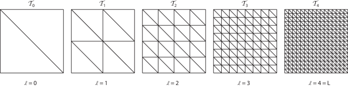
Fig. 3: A hierarchical triangulation, ${\mathcal{T}}_{\ell}$, $\ell=0,1,\ldots,L$, of a square domain $\Omega$. Here $L=4$, though in typical calculations we may use $L=8$ or 9.

In this section we provide some numerical experiments to gauge the accuracy and reliability of the fully discrete finite element method developed in the previous sections. For the experiments we take $V_{h}=W_{h}=S_{h}^{1}$ for simplicity. We use a square domain $\Omega=(0,1)^{2}$ and take ${\mathcal{T}}_{h}$ to be a regular triangulation of $\Omega$ consisting of right isosceles triangles, as depicted in Fig. 3. We use a nonlinear multigrid method, which is detailed in Appendix A, to solve the scheme (56)–(59) at each time step. We perform a battery of three tests on the scheme. First, we measure numerical convergence of the scheme in the presence of added, artificial source terms. Second, we measure the numerical convergence of the scheme without source terms using a Cauchy-convergence method. Third, we conduct a test of spinodal decomposition using varying values of the excess surface tension $\gamma$, and demonstrate the discrete energy dissipation and mass conservation properties of the scheme.

$h$	$\left\|e_{\varphi}\right\|_{L^{2}}$	rate	$\left\|e_{\mu}\right\|_{L^{2}}$	rate	$\left\|e_{p}\right\|_{L^{2}}$	rate
$\nicefrac{{\sqrt{2}}}{{16}}$	$8.683\times 10^{-3}$	–	$1.088\times 10^{-2}$	–	$1.270\times 10^{-2}$	–
$\nicefrac{{\sqrt{2}}}{{32}}$	$1.850\times 10^{-3}$	2.23	$2.701\times 10^{-3}$	2.01	$2.479\times 10^{-3}$	2.35
$\nicefrac{{\sqrt{2}}}{{64}}$	$4.568\times 10^{-4}$	2.01	$6.759\times 10^{-4}$	2.00	$5.759\times 10^{-4}$	2.11
$\nicefrac{{\sqrt{2}}}{{128}}$	$1.141\times 10^{-4}$	2.00	$1.691\times 10^{-4}$	2.00	$1.413\times 10^{-4}$	2.03
$\nicefrac{{\sqrt{2}}}{{256}}$	$2.852\times 10^{-5}$	2.00	$4.227\times 10^{-5}$	2.00	$3.515\times 10^{-5}$	2.00

Table 1: $L^{2}$ convergence test. The final time is $T=1.0$, and the refinement path is taken to be $\tau=25.6h^{2}$. The other parameters are $\varepsilon=\gamma=1.0$; $\Omega=(0,1)^{2}$. The global error at $T$ is expected to be $\mathcal{O}(\tau)+\mathcal{O}\left(h^{2}\right)=\mathcal{O}\left(h^{2}\right)$, and this is confirmed.

$h$	$\left\|e_{\varphi}\right\|_{H^{1}}$	rate	$\left\|e_{\mu}\right\|_{H^{1}}$	rate	$\left\|e_{p}\right\|_{H^{1}}$	rate
$\nicefrac{{\sqrt{2}}}{{16}}$	$2.886\times 10^{-1}$	–	$2.907\times 10^{-1}$	–	$2.943\times 10^{-1}$	–
$\nicefrac{{\sqrt{2}}}{{32}}$	$1.455\times 10^{-1}$	0.99	$1.462\times 10^{-1}$	0.99	$1.466\times 10^{-1}$	1.01
$\nicefrac{{\sqrt{2}}}{{64}}$	$7.290\times 10^{-2}$	1.00	$7.320\times 10^{-2}$	1.00	$7.313\times 10^{-2}$	1.00
$\nicefrac{{\sqrt{2}}}{{128}}$	$3.647\times 10^{-2}$	1.00	$3.660\times 10^{-2}$	1.00	$3.653\times 10^{-2}$	1.00
$\nicefrac{{\sqrt{2}}}{{256}}$	$1.824\times 10^{-2}$	1.00	$1.839\times 10^{-2}$	1.00	$1.826\times 10^{-2}$	1.00

Table 2: $H^{1}$ convergence test. The final time is $T=1.0$, and the refinement path is taken to be $\tau=1.6h$. The other parameters are $\varepsilon=\gamma=1.0$; $\Omega=(0,1)^{2}$. The global error at $T$ is expected to be $\mathcal{O}(\tau)+\mathcal{O}(h)=\mathcal{O}(h)$, and this is confirmed.

For the convergence of the problem with source terms, we solve a problem of the following form: find $\left(p^{m}_{h},\mu^{m}_{h},\varphi^{m}_{h}\right)\in\mathring{V}_{h}\times V_{h}\times V_{h}$, such that

(121) $$\bigl{(}\nabla p^{m}_{h}+\gamma\varphi_{h}^{m-1}\nabla\mu_{h}^{m},\nabla q_{h}\bigr{)} =\left(s_{1}({\bf x},t_{m}),q_{h}\right) \quad\forall\ q_{h}\in V_{h},$$

(122) $$\left(d_{t}\varphi^{m}_{h},\nu_{h}\right)+\varepsilon\bigl{(}\nabla\mu_{h}^{m},\nabla\nu_{h}\bigr{)}\hskip 72.26999pt$$

$$+\left(\varphi_{h}^{m-1}[\nabla p^{m}_{h}+\gamma\varphi_{h}^{m-1}\nabla\mu_{h}^{m}],\nabla\nu_{h}\right) =\left(s_{2}({\bf x},t_{m}),\nu_{h}\right) \quad\forall\ \nu_{h}\in V_{h},$$

(123) $$\left(\mu_{h}^{m},\psi_{h}\right)-\varepsilon\left(\nabla\varphi^{m}_{h},\nabla\psi_{h}\right)-\frac{1}{\varepsilon}\left(f_{h}^{m},\psi_{h}\right) =\left(s_{3}({\bf x},t_{m}),\psi_{h}\right) \quad\forall\ \psi_{h}\in V_{h},$$

(124) $$\varphi_{h}^{0} =\varphi_{0h},$$

for $m=1,\ldots,M$, where the source terms are chosen so that the solution of the corresponding continuous problem is precisely

(125) $$p(x,y,t)=\mu(x,y,t)=\varphi(x,y,t)=\cos(\pi t)\cdot g(x)\cdot g(y),$$

with $g(\xi)=16\xi^{2}(\xi-1)^{2}$. The initial data are precisely given by $\varphi_{0h}=\mathcal{I}_{h}\left(\varphi(\,\cdot\,,0)\right)$, where $\mathcal{I}_{h}:H^{2}\left(\Omega\right)\to V_{h}$ is the standard nodal interpolation operator. All integrations are done exactly using the appropriate Gauss-quadrature rules. This is of course made possible since we are using polynomials in space. The exact values of all of the other parameters used in the test are given in the captions of Tabs. 1 and 2. The results of an $L^{2}$ error analysis using a quadratic refinement path are found in Tab. 1 and confirm the expected optimal second-order convergence rate in this case. The results of an $H^{1}$ error analysis using a linear refinement path are found in Tab. 2 and confirm the expected optimal first-order convergence rate for this case. Notice that the approximations $p^{m}_{h}$, $\varphi^{m}_{h}$, and $\mu^{m}_{h}$ all appear to converge at the same optimal rates, in both cases.

$h_{c}$	$h_{f}$	$\left\|\delta_{\varphi}\right\|_{L^{2}}$	rate	$\left\|\delta_{\mu}\right\|_{L^{2}}$	rate	$\left\|\delta_{p}\right\|_{L^{2}}$	rate
$\nicefrac{{\sqrt{2}}}{{16}}$	$\nicefrac{{\sqrt{2}}}{{32}}$	$5.514\times 10^{-2}$	–	$2.890\times 10^{-1}$	–	$3.099\times 10^{-2}$	–
$\nicefrac{{\sqrt{2}}}{{32}}$	$\nicefrac{{\sqrt{2}}}{{64}}$	$2.165\times 10^{-2}$	1.35	$1.229\times 10^{-1}$	1.23	$1.148\times 10^{-2}$	1.43
$\nicefrac{{\sqrt{2}}}{{64}}$	$\nicefrac{{\sqrt{2}}}{{128}}$	$6.284\times 10^{-3}$	1.78	$3.588\times 10^{-2}$	1.78	$3.250\times 10^{-3}$	1.82
$\nicefrac{{\sqrt{2}}}{{128}}$	$\nicefrac{{\sqrt{2}}}{{256}}$	$1.636\times 10^{-3}$	1.94	$9.327\times 10^{-3}$	1.94	$8.420\times 10^{-4}$	1.95
$\nicefrac{{\sqrt{2}}}{{256}}$	$\nicefrac{{\sqrt{2}}}{{512}}$	$4.132\times 10^{-4}$	1.99	$2.355\times 10^{-3}$	1.99	$2.128\times 10^{-4}$	1.98

Table 3: $L^{2}$ Cauchy convergence test. The final time is $T=4.0\times 10^{-2}$, and the refinement path is taken to be $\tau=1.024h^{2}$. The other parameters are $\varepsilon=6.25\times 10^{-2}$; $\gamma=1.25\times 10^{-1}$; $\Omega=(0,1)^{2}$. The Cauchy difference is defined via $\delta_{\varphi}:=\varphi_{h_{f}}-\varphi_{h_{c}}$, where the approximations are evaluated at time $t=T$, and analogously for $\delta_{\mu}$, and $\delta_{p}$. The norm of the Cauchy difference at $T$ is expected to be $\mathcal{O}(\tau)+\mathcal{O}\left(h^{2}\right)=\mathcal{O}\left(h^{2}\right)$.

$h_{c}$	$h_{f}$	$\left\|\delta_{\varphi}\right\|_{H^{1}}$	rate	$\left\|\delta_{\mu}\right\|_{H^{1}}$	rate	$\left\|\delta_{p}\right\|_{H^{1}}$	rate
$\nicefrac{{\sqrt{2}}}{{16}}$	$\nicefrac{{\sqrt{2}}}{{32}}$	$8.569\times 10^{-1}$	–	$1.301\times 10^{-0}$	–	$8.371\times 10^{-2}$	–
$\nicefrac{{\sqrt{2}}}{{32}}$	$\nicefrac{{\sqrt{2}}}{{64}}$	$4.160\times 10^{-1}$	1.04	$6.295\times 10^{-1}$	1.04	$3.715\times 10^{-1}$	1.17
$\nicefrac{{\sqrt{2}}}{{64}}$	$\nicefrac{{\sqrt{2}}}{{128}}$	$2.061\times 10^{-1}$	1.01	$3.111\times 10^{-1}$	1.02	$1.779\times 10^{-2}$	1.06
$\nicefrac{{\sqrt{2}}}{{128}}$	$\nicefrac{{\sqrt{2}}}{{256}}$	$1.029\times 10^{-1}$	1.00	$1.554\times 10^{-1}$	1.00	$8.834\times 10^{-3}$	1.01
$\nicefrac{{\sqrt{2}}}{{256}}$	$\nicefrac{{\sqrt{2}}}{{512}}$	$5.146\times 10^{-2}$	1.00	$7.777\times 10^{-2}$	1.00	$4.422\times 10^{-3}$	1.00

Table 4: $H^{1}$ Cauchy convergence test. The final time is $T=4.0\times 10^{-2}$, and the refinement path is taken to be $\tau=2.0\times 10^{-3}h$. The other parameters are $\varepsilon=6.25\times 10^{-2}$; $\gamma=1.25\times 10^{-1}$; $\Omega=(0,1)^{2}$. The norm of the Cauchy difference at $T$ is expected to be $\mathcal{O}(\tau)+\mathcal{O}\left(h\right)=\mathcal{O}\left(h\right)$.

We now give the results of a test without any artificial sources. In other words, we solve the scheme (121)–(123) with $s_{i}\equiv 0$, $i=1,2,3$. The initial data are taken to be

(126) $$\varphi_{0h}=\mathcal{I}_{h}\left(\frac{\big{[}1.0-\cos(4.0\pi x)\big{]}\cdot\big{[}1.0-\cos(2.0\pi y)\big{]}}{2}-1.0\right),$$

and the parameters are given in the captions of Tabs. 3 and 4. Note that in this case we are not in possession of the exact solutions. To circumvent this, we measure the difference of the computed solutions at successive resolutions. Specifically, we compute the rate at which the Cauchy difference $\delta_{\psi}:=\psi^{M_{f}}_{h_{f}}-\psi^{M_{c}}_{h_{c}}$ converges to zero, where $h_{f}=2h_{c}$, $\tau_{f}=2^{p}\tau_{c}$ ($p=1$ for a linear refinement path and $p=2$ for a quadratic refinement path), and $\tau_{f}M_{f}=\tau_{c}M_{c}=T$. A quadratic refinement path, i.e., $\tau=Ch^{2}$, is taken when measurements are made in the $L^{2}$ norm, and a linear refinement path, i.e., $\tau=Ch$, when measurements are made in the $H^{1}$ norm. The results of an $L^{2}$ Cauchy error analysis are found in Tab. 3 and confirm second-order convergence in this case. The results of an $H^{1}$ Cauchy error analysis are found in Tab. 4 and confirm first-order convergence in this case.

Our final test is a simulation of spinodal decomposition with different values of $\gamma$. Specifically, we solve the scheme (121)–(123) with $s_{i}\equiv 0$, $i=1,2,3$, and with three values of $\gamma$; namely, $\gamma=0$, which yields the familiar Cahn-Hilliard model; $\gamma=0.01$; and $\gamma=0.04$. Furthermore, we take $\varepsilon=0.01$, $h=\frac{\sqrt{2}}{256}$, $\tau=1\times 10^{-3}$, and $T=0.1$. We use the same randomized initial data for the three simulations represented in Fig. 1, where the average value of $\varphi$ is approximately $-0.1$. As expected, the mixture phase separates into domains wherein $\varphi\approx-1$ and $\varphi\approx+1$. Afterwards the system coarsens, as larger phase regions grow at the expense of smaller ones. The energy for the three simulations is displayed in Fig. 2. A general trend emerges, where, at least at early times, the energy decreases faster and the coarsening process is appears to be accelerated as the excess surface tension $\gamma$ increases. This behavior is expected and was observed in similar finite difference calculations undertaken in [28].

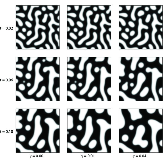
Fig. 1: Spinodal decomposition for three values of $\gamma$. The domain is $\Omega=(0,1)\times(0,1)$ and $\varepsilon=0.01$. The initial data are exactly the same for the three simulations. The time step size is $\tau=1.0\times 10^{-3}$, and $h=\nicefrac{{\sqrt{2}}}{{256}}$. We use a uniform mesh, as in Fig. 3. The corresponding energy plots are shown in Fig. 2. The average value of $\varphi$ for all three simulations is approximately $-0.1$. For $\gamma=0.01$, the mass variation over the simulated time is only $1\times 10^{-12}$. The max and min values of $\varphi$ are very near the values $+1$ and $-1$, respectively.

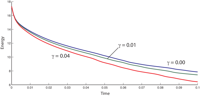
Fig. 2: Energy plots for the spinodal decomposition simulations depicted in Fig. 1. The parameters for the simulations are given in the caption of Fig. 1. The energy is observed to decrease at each time step. The general trend, at least at early times, is that the energy decreases faster with increasing values of the excess surface tension $\gamma$.

Note that we have proved that (at the theoretical level) the energy is non-increasing at each time step. This is observed in our computations. In addition to this, the mass, i.e, $\int_{\Omega}\varphi_{h}\,dx$, at the theoretical level is expected to be unchanging from one time step to the next. On the practical level, we observe very little mass variation. For example, for the $\gamma=0.01$ case depicted in Fig. 1, where initially $\int_{\Omega}\varphi_{0h}\,dx\approx-0.1$, we observe mass variation of only $1\times 10^{-12}$ over the whole of the simulation time. Note that our multigrid iteration stopping tolerance is of the same order, namely, $tol=1\times 10^{-12}$ in (161).

Appendix A Nonlinear Multigrid Solver

In this appendix we give the full details of the nonlinear multigrid solver that is used to march the scheme in time. Suppose $\Omega\subseteq\mathbb{R}^{2}$ is polygonal, and assume that ${\mathcal{T}}_{\ell}$, $\ell=0,1,\ldots,L$, is a hierarchy of nested triangulations of $\Omega$ as suggested in Fig. 1. In particular, ${\mathcal{T}}_{\ell}$ is obtained by subdividing the triangles of ${\mathcal{T}}_{\ell-1}$ into 4 congruent sub-triangles. Note that $h_{\ell-1}=2h_{\ell}$, $\ell=1,\ldots,L$, and that $\left\{{\mathcal{T}}_{\ell}\right\}$ is a quasi-uniform family. For simplicity, we shall use $P_{1}$ finite element spaces and use the same space for the pressure as is used for the other variables. We define

$$V_{\ell}=\left\{v\in C^{0}(\overline{\Omega})\ \middle|\ v|_{K}\in P_{1}(K)\ \ \forall K\in{\mathcal{T}}_{\ell}\right\},$$

for $\ell=0,\ldots,L$ and observe the nested space chain $V_{0}\subset V_{1}\subset V_{3}\subset\cdots\subset V_{L}$. Because of this nestedness, there is a natural injection operation $I_{\ell-1,\ell}:V_{\ell-1}\hookrightarrow V_{\ell}$ defined by $I_{\ell-1,\ell}(v)=v$, for all $v\in V_{\ell-1}$, $\ell=1,\ldots,L$. Now, let $B_{\ell}=\left\{u_{\ell,i}(\mathbf{x})\right\}_{i=1}^{N_{\ell}}$ be the nodal basis for $V_{\ell}$, $\ell=0,1,\ldots,L$. In other words, $u_{\ell,j}\left({\bf x}_{\ell,i}\right)=\delta_{i,j}$, where $\left\{{\bf x}_{\ell,i}\right\}_{i=1}^{N_{\ell}}$ are the nodes of ${\mathcal{T}}_{\ell}$. We have level-wise representations of the unknowns of the form

(127) $$\varphi_{\ell}(\mathbf{x})=\sum_{i=1}^{N_{\ell}}\varphi_{\ell,i}u_{\ell,i}(\mathbf{x})\iff\mbox{\boldmath$\varphi$}_{\ell}=\left(\varphi_{\ell,1},\varphi_{\ell,2},\ldots,\varphi_{\ell,N_{\ell}}\right)^{T},$$

and similarly for $\mu_{\ell}(\mathbf{x})$ and $p_{\ell}(\mathbf{x})$. Define the prolongation matrix via ${\mathsf{P}}_{\ell-1,\ell}:={\mathsf{I}}_{\ell-1,\ell}$, where ${\mathsf{I}}_{\ell-1,\ell}$ is the $N_{\ell}\times N_{\ell-1}$ matrix representation of the injection operator $I_{\ell-1,\ell}$ with respect to the bases $B_{\ell-1}$ and $B_{\ell}$. There are two restriction operations — i.e., operations transferring information from the finer space $V_{\ell}$ to the coarser space $V_{\ell-1}$ — that we shall use. The first is called the canonical restriction and, in matrix form, is the $N_{\ell-1}\times N_{\ell}$ matrix defined via ${\mathsf{R}}_{\ell,\ell-1}:={\mathsf{I}}_{\ell-1,\ell}^{T}$ [6, 7]. The second is defined via

(128) $$\hat{R}_{\ell,\ell-1}(v)=\sum_{i=1}^{N_{\ell-1}}v\left({\bf x}_{\ell-1,i}\right)u_{\ell-1,i}\left({\bf x}\right)\quad\forall v\in V_{\ell},$$

where the points ${\bf x}_{\ell-1,i}$ are the nodes of the mesh ${\mathcal{T}}_{\ell-1}$. Note that $\left\{{\bf x}_{\ell-1,i}\right\}_{i=1}^{N_{\ell-1}}\subset\left\{{\bf x}_{\ell,i}\right\}_{i=1}^{N_{\ell}}$ by construction. By $\hat{{\mathsf{R}}}_{\ell,\ell-1}$ we denote the matrix representation of $\hat{R}_{\ell,\ell-1}$ with respect to the bases $B_{\ell}$ and $B_{\ell-1}$.

In the present framework, our nonlinear finite element scheme is defined on the finest level, $\ell=L$, as follows: find the triple $(p_{L},\mu_{L},\varphi_{L})\in\mathring{V}_{L}\times V_{L}\times V_{L}$ such that

(129) $$\bigl{(}\nabla p_{L}+\gamma\varphi_{L}^{m-1}\nabla\mu_{L},\nabla q_{L}\bigr{)} =0 \quad\forall q_{L}\in\mathring{V}_{L}\ ,$$

(130) $$\left(\varphi_{L},\nu_{L}\right)+\tau\varepsilon\bigl{(}\nabla\mu_{L},\nabla\nu_{L}\bigr{)}\hskip 72.26999pt$$

$$+\tau\left(\varphi_{L}^{m-1}\left[\nabla p_{L}+\gamma\varphi_{L}^{m-1}\nabla\mu_{L}\right],\nabla\nu_{L}\right) =\left(\varphi_{L}^{m-1},\nu_{L}\right) \quad\forall\nu_{L}\in V_{L},$$

(131) $$\left(\mu_{L},\psi_{L}\right)-\varepsilon\left(\nabla\varphi_{L},\nabla\psi_{L}\right)-\frac{1}{\varepsilon}\left(\left(\varphi_{L}\right)^{2}\varphi_{L},\psi_{L}\right) =-\frac{1}{\varepsilon}\left(\varphi_{L}^{m-1},\psi_{L}\right) \quad\forall\psi_{L}\in V_{L},$$

where $\varphi_{L}^{m-1}\in V_{L}$ is given. We have dropped the superscript $m$ (the time step index) on the unknowns for simplicity. Theorem 8 guarantees that this problem always has a unique solution. The nonlinear system (129)–(131) may be written as

(132) $${\mathsf{A}}_{L}\mathbf{p}_{L}+\gamma{\mathsf{C}}_{L}\mbox{\boldmath$\mu$}_{L} = {\bf 0},$$

(133) $${\mathsf{M}}_{L}\mbox{\boldmath$\varphi$}_{L}+\tau\left(\varepsilon{\mathsf{A}}_{L}+\gamma{\mathsf{B}}_{L}\right)\mbox{\boldmath$\mu$}_{L}+\tau{\mathsf{C}}_{L}\mathbf{p}_{L} = {\mathsf{M}}_{L}\mbox{\boldmath$\varphi$}_{L}^{m-1},$$

(134) $$\varepsilon{\mathsf{A}}_{L}\mbox{\boldmath$\varphi$}_{L}+\frac{1}{\varepsilon}{\mathsf{Q}}_{L}\left(\mbox{\boldmath$\varphi$}_{L}\right)\mbox{\boldmath$\varphi$}_{L}-{\mathsf{M}}_{L}\mbox{\boldmath$\mu$}_{L} = \frac{1}{\varepsilon}{\mathsf{M}}_{L}\mbox{\boldmath$\varphi$}_{L}^{m-1},$$

where ${\mathsf{A}}_{L}$, ${\mathsf{B}}_{L}$, ${\mathsf{C}}_{L}$, ${\mathsf{M}}_{L}$, and ${\mathsf{Q}}_{L}\left(\mbox{\boldmath$\varphi$}_{L}\right)$ are $N_{L}\times N_{L}$ matrices whose components are

(135) $$\left[{\mathsf{A}}_{L}\right]_{i,j} :=\left(\nabla u_{L,j},\nabla u_{L,i}\right), \quad\left[{\mathsf{B}}_{L}\right]_{i,j} :=\left(\left(\varphi_{L}^{m-1}\right)^{2}\nabla u_{L,j},\nabla u_{L,i}\right),$$

(136) $$\left[{\mathsf{C}}_{L}\right]_{i,j} :=\left(\varphi_{L}^{m-1}\nabla u_{L,j},\nabla u_{L,i}\right), \quad\left[{\mathsf{M}}_{L}\right]_{i,j} :=\left(u_{L,j},u_{L,i}\right),$$

(137) $$\left[{\mathsf{Q}}_{L}\left(\mbox{\boldmath$\varphi$}_{L}\right)\right]_{i,j} :=\left(\left(\varphi_{L}\right)^{2}u_{L,j},u_{L,i}\right).$$

We solve (132)–(134) using a nonlinear multigrid method [6, Ch. 5, §6]. This requires that we split the equations into source (${\bf s}$) and operator (${\mathsf{N}}$) terms:

(138) $${\bf s}_{L}^{(1)} :={\bf 0}, \quad{\mathsf{N}}_{L}^{(1)}\left(\mbox{\boldmath$\phi$}_{L}\right) :={\mathsf{A}}_{L}\mathbf{p}_{L}+\gamma{\mathsf{C}}_{L}\mbox{\boldmath$\mu$}_{L}\ ,$$

(139) $${\bf s}_{L}^{(2)} :={\mathsf{M}}_{L}\mbox{\boldmath$\varphi$}_{L}^{m-1}, \quad{\mathsf{N}}_{L}^{(2)}\left(\mbox{\boldmath$\phi$}_{L}\right) :={\mathsf{M}}_{L}\mbox{\boldmath$\varphi$}_{L}+\tau\left(\varepsilon{\mathsf{A}}_{L}+\gamma{\mathsf{B}}_{L}\right)\mbox{\boldmath$\mu$}_{L}+\tau{\mathsf{C}}_{L}\mathbf{p}_{L},$$

(140) $${\bf s}_{L}^{(3)} :=\frac{1}{\varepsilon}{\mathsf{M}}_{L}\mbox{\boldmath$\varphi$}_{L}^{m-1}, \quad{\mathsf{N}}_{L}^{(3)}\left(\mbox{\boldmath$\phi$}_{L}\right) :=\varepsilon{\mathsf{A}}_{L}\mbox{\boldmath$\varphi$}_{L}+\frac{1}{\varepsilon}{\mathsf{Q}}_{L}\left(\mbox{\boldmath$\varphi$}_{L}\right)\mbox{\boldmath$\varphi$}_{L}-{\mathsf{M}}_{L}\mbox{\boldmath$\mu$}_{L},$$

where $\mbox{\boldmath$\phi$}_{L}:=\left[\mathbf{p}_{L},\mbox{\boldmath$\mu$}_{L},\mbox{\boldmath$\varphi$}_{L}\right]$ is the $N_{L}\times 3$ array of unknowns. We must also define a “consistent” version of the nonlinear operator on all of the coarser levels. There are a number of ways to proceed in this task [6]; we choose the following path. Suppose that $\ell\in\left\{0,1,\ldots,L-1\right\}$ is given. We restrict the known solution from the previous time step to the coarser levels via

(141) $$\mbox{\boldmath$\varphi$}_{\ell}^{m-1}:=\prod_{j=\ell+1}^{L}\hat{{\mathsf{R}}}_{j,j-1}\mbox{\boldmath$\varphi$}_{L}^{m-1} = \left(\varphi_{\ell,1}^{m-1},\varphi_{\ell,2}^{m-1},\ldots\varphi_{\ell,N_{\ell}}^{m-1}\right)^{T},$$

$$\iff\varphi_{\ell}^{m-1}(\mathbf{x}) = \sum_{i=1}^{N_{\ell}}\varphi_{\ell,i}^{m-1}u_{\ell,i}(\mathbf{x}).$$

Now, given any $\psi_{\ell}\in V_{\ell}$ with the representation

(142) $$\mbox{\boldmath$\psi$}_{\ell}=\left(\psi_{\ell,1},\psi_{\ell,2},\ldots,\psi_{\ell,N_{\ell}}\right)^{T}\iff\psi_{\ell}(\mathbf{x})=\sum_{i=1}^{N_{\ell}}\psi_{\ell,i}u_{\ell,i}(\mathbf{x}),$$

we define

(143) $$\left[{\mathsf{A}}_{\ell}\right]_{i,j} :=\left(\nabla u_{\ell,j},\nabla u_{\ell,i}\right), \quad\left[{\mathsf{B}}_{\ell}\right]_{i,j} :=\left(\left(\varphi_{\ell}^{m-1}\right)^{2}\nabla u_{\ell,j},\nabla u_{\ell,i}\right),$$

(144) $$\left[{\mathsf{C}}_{\ell}\right]_{i,j} :=\left(\varphi_{\ell}^{m-1}\nabla u_{\ell,j},\nabla u_{\ell,i}\right), \quad\left[{\mathsf{M}}_{\ell}\right]_{i,j} :=\left(u_{\ell,j},u_{\ell,i}\right),$$

(145) $$\left[{\mathsf{Q}}_{\ell}\left(\mbox{\boldmath$\psi$}_{\ell}\right)\right]_{i,j} :=\left(\left(\psi_{\ell}\right)^{2}u_{\ell,j},u_{\ell,i}\right).$$

Observe that

(146) $${\mathsf{A}}_{\ell}={\mathsf{R}}_{\ell+1,\ell}{\mathsf{A}}_{\ell+1}{\mathsf{P}}_{\ell,\ell+1},\quad{\mathsf{M}}_{\ell}={\mathsf{R}}_{\ell+1,\ell}{\mathsf{M}}_{\ell+1}{\mathsf{P}}_{\ell,\ell+1},$$

which is standard in the finite element setting [6, 7] and is the reason for the term “canonical” describing ${\mathsf{R}}_{\ell+1,\ell}$. On the other hand,

(147) $${\mathsf{B}}_{\ell}\approx{\mathsf{R}}_{\ell+1,\ell}{\mathsf{B}}_{\ell+1}{\mathsf{P}}_{\ell,\ell+1},\quad{\mathsf{C}}_{\ell}\approx{\mathsf{R}}_{\ell+1,\ell}{\mathsf{C}}_{\ell+1}{\mathsf{P}}_{\ell,\ell+1}.$$

(Note that we could have recursively defined ${\mathsf{B}}_{\ell}={\mathsf{R}}_{\ell+1,\ell}{\mathsf{B}}_{\ell+1}{\mathsf{P}}_{\ell,\ell+1}$, and similarly for ${\mathsf{C}}_{\ell}$. But it turns out that this is an unnecessary complication from the point of view of the convergence of the algorithm.) Finally, we have

(148) $${\mathsf{N}}_{\ell}^{(1)}\left(\mbox{\boldmath$\xi$}_{\ell}\right) := {\mathsf{A}}_{\ell}\mathbf{q}_{\ell}+\gamma{\mathsf{C}}_{\ell}\mbox{\boldmath$\nu$}_{\ell},$$

(149) $${\mathsf{N}}_{\ell}^{(2)}\left(\mbox{\boldmath$\xi$}_{\ell}\right) := {\mathsf{M}}_{\ell}\mbox{\boldmath$\psi$}_{\ell}+\tau\left(\varepsilon{\mathsf{A}}_{\ell}+\gamma{\mathsf{B}}_{\ell}\right)\mbox{\boldmath$\nu$}_{\ell}+\tau{\mathsf{C}}_{\ell}\mathbf{q}_{\ell},$$

(150) $${\mathsf{N}}_{\ell}^{(3)}\left(\mbox{\boldmath$\xi$}_{\ell}\right) := \varepsilon{\mathsf{A}}_{\ell}\mbox{\boldmath$\varphi$}_{\ell}+\frac{1}{\varepsilon}{\mathsf{Q}}_{\ell}\left(\mbox{\boldmath$\psi$}_{\ell}\right)\mbox{\boldmath$\psi$}_{\ell}-{\mathsf{M}}_{\ell}\mbox{\boldmath$\nu$}_{\ell},$$

where $\mbox{\boldmath$\xi$}_{\ell}:=\left[\mathbf{q}_{\ell},\mbox{\boldmath$\nu$}_{\ell},\mbox{\boldmath$\psi$}_{\ell}\right]$ is any given $N_{\ell}\times 3$ array of unknowns.

We are now in a position to define the recursive nonlinear multigrid V-Cycle operator [6, Ch. 5, §6], which is the heart of our solver. In the following the superscript $k$ is the V-Cycle loop index (not the time step index). Let $\mbox{\boldmath$\phi$}_{\ell}^{k-1}:=\left[\mathbf{p}_{\ell}^{k-1},\mbox{\boldmath$\mu$}_{\ell}^{k-1},\mbox{\boldmath$\varphi$}_{\ell}^{k-1}\right]$ denote the current, level-$\ell$ multigrid iterate. For any $N_{\ell}\times 3$ array of unknowns $\mbox{\boldmath$\xi$}_{\ell}$, define ${\mathsf{N}}_{\ell}\left(\mbox{\boldmath$\xi$}_{\ell}\right):=\left[{\mathsf{N}}_{\ell}^{(1)}\left(\mbox{\boldmath$\xi$}_{\ell}\right),{\mathsf{N}}_{\ell}^{(2)}\left(\mbox{\boldmath$\xi$}_{\ell}\right),{\mathsf{N}}_{\ell}^{(3)}\left(\mbox{\boldmath$\xi$}_{\ell}\right)\right]$, and ${\bf s}_{\ell}:=\left[{\bf s}_{\ell}^{(1)},{\bf s}_{\ell}^{(2)},{\bf s}_{\ell}^{(3)}\right]$. Note that these last two objects are $N_{\ell}\times 3$ arrays by design. We define the action of the recursive nonlinear multigrid V-Cycle operator

(151) $$\mbox{\boldmath$\phi$}_{\ell}^{k}=\mbox{NMGM}\left(\ell,\mbox{\boldmath$\phi$}_{\ell}^{k-1},{\mathsf{N}}_{\ell},{\bf s}_{\ell},\lambda\right)$$

in the following 3 steps:

1. Pre-smoothing:

   • Given $\mbox{\boldmath$\phi$}_{\ell}^{k-1}$, compute a smoothed level-$\ell$ approximation $\bar{}\mbox{\boldmath$\phi$}_{\ell}$:

     (152) $$\bar{}\mbox{\boldmath$\phi$}_{\ell}={\mathcal{S}}^{\lambda}\left(\mbox{\boldmath$\phi$}_{\ell}^{k-1},{\mathsf{N}}_{\ell},{\bf s}_{\ell}\right),$$

     where ${\mathcal{S}}$ is a smoothing (or relaxation) operator, and $\lambda>0$ is the number of smoothing sweeps.

2. Coarse-grid correction:

   • Compute coarse-level initial iterate:

     (153) $$\bar{}\mbox{\boldmath$\phi$}_{\ell-1}=\hat{{\mathsf{R}}}_{\ell,\ell-1}\bar{}\mbox{\boldmath$\phi$}_{\ell}\ .$$

   • Compute the coarse-level right-hand side:

     (154) $${\bf s}_{\ell-1}={\mathsf{R}}_{\ell,\ell-1}\left({\bf s}_{\ell}-{\mathsf{N}}_{\ell}(\bar{}\mbox{\boldmath$\phi$}_{\ell})\right)+{\mathsf{N}}_{\ell-1}\left(\bar{}\mbox{\boldmath$\phi$}_{\ell-1}\right).$$

   • Compute an approximate solution $\hat{\mbox{\boldmath$\xi$}}_{\ell-1}$ of the following coarse grid equation:

     (155) $${\mathsf{N}}_{\ell-1}(\mbox{\boldmath$\xi$}_{\ell-1})={\bf s}_{\ell-1}.$$

     Note that this equation is uniquely solvable by Theorem 8.

     • If $\ell=1$ employ $\lambda$ smoothing steps:

       (156) $$\hat{}\mbox{\boldmath$\xi$}_{0}=\mathcal{S}^{\lambda}\left(\bar{}\mbox{\boldmath$\phi$}_{0},{\mathsf{N}}_{0},{\bf s}_{0}\right).$$

     • If $\ell>1$ get an approximate solution to Eq. (155) using $\bar{}\mbox{\boldmath$\phi$}_{\ell-1}$ as initial guess:

       (157) $$\hat{\mbox{\boldmath$\xi$}}_{\ell-1}=\mbox{NMGM}\left(\ell-1,\bar{}\mbox{\boldmath$\phi$}_{\ell-1},{\mathsf{N}}_{\ell-1},{\bf s}_{\ell-1},\lambda\right).$$

   • Compute the coarse-grid correction:

     (158) $$\hat{\mbox{\boldmath$\phi$}}_{\ell-1}=\hat{\mbox{\boldmath$\xi$}}_{\ell-1}-\bar{\mbox{\boldmath$\phi$}}_{\ell-1}.$$

   • Compute the coarse-grid-corrected approximation at level $k$:

     (159) $$\hat{\mbox{\boldmath$\phi$}}_{\ell}={\mathsf{P}}_{\ell-1,\ell}\hat{\mbox{\boldmath$\phi$}}_{\ell-1}+\bar{\mbox{\boldmath$\phi$}}_{\ell}.$$

3. Post-smoothing:

   • Finally, compute $\mbox{\boldmath$\phi$}_{\ell}^{k}$ by applying $\lambda$ smoothing steps:

     (160) $$\mbox{\boldmath$\phi$}_{\ell}^{k}=\mathcal{S}^{\lambda}\left(\hat{\mbox{\boldmath$\phi$}}_{\ell},{\mathsf{N}}_{\ell},{\bf s}_{\ell}\right).$$

When

(161) $$\sqrt{\frac{1}{3N_{L}}\sum_{j=1}^{3}\sum_{i=1}^{N_{L}}\left(\left[{\bf s}^{(j)}_{L}-{\mathsf{N}}^{(j)}_{L}\left(\mbox{\boldmath$\phi$}_{L}^{k}\right)\right]_{i}\right)^{2}\ }<tol$$

we stop iterating and set $\mbox{\boldmath$\phi$}_{L}^{k}\to\mbox{\boldmath$\phi$}_{L}=\left[\mathbf{p}_{L},\mbox{\boldmath$\mu$}_{L},\mbox{\boldmath$\varphi$}_{L}\right]$, the fine-level solution. For smoothing, we use a nonlinear block Gauß-Seidel method, like that discussed in [28] for a similar finite-difference nonlinear multigrid method. The exact details are omitted for brevity, but the principal idea is that the nodal values $\left(p_{\ell,i},\mu_{\ell,i},\varphi_{\ell,i}\right)$ are always obtained simultaneously in the smoothing operation. We use $\lambda=2$ or 3 in the smoothing step.

References

• [1] R.ย A. Adams, Sobolev Spaces, Academic press, New York, 1975.
• [2] D. M. Anderson and G. B. McFadden, Diffuse-interface method in fluid mechanics, Annual Review of Fluid Mech, vol. 30 (1998), pp. 139โ€“165.
• [3] N. D. Alikakos, P. W. Bates, and X. Chen, Convergence of the Cahn-Hilliard equation to the Hele-Shaw model, Arch. Rational Mech. Anal., 128 (1994), pp. 165โ€“205.
• [4] J. Bear, Dynamics of Fluids in Porous Media, Dover Publications, Inc., New York, 1972.
• [5] H. Blum and R. Rannacher, On the boundary value problem of biharmonic operator on domains with angular corners, Math. Methods Appl. Sci., 2 (1980), pp. 556โ€“581.
• [6] D. Braess, Finite Elements: Theory, Fast Solvers, and Applications in Solid Mechanics, third edition, Cambridge, 2007.
• [7] S. C. Brenner and L. R. Scott, The Mathematical Theory of Finite Element Methods, third edition, Springer, 2008.
• [8] J.ย W. Cahn and J.ย E. Hilliard, Free energy of a nonuniform system I. Interfacial free energy, J. Chem. Phys., 28 (1958), pp. 258โ€“267.
• [9] P.ย G. Ciarlet, The Finite Element Method for Elliptic Problems, North-Holland, Amsterdam, 1978.
• [10] C.ย M. Elliott, D.ย A. French, and F.ย A. Milner, A second order splitting method for the Cahn-Hilliard equation, Numer. Math., 54 (1989), pp. 575โ€“590.
• [11] C.ย M. Elliott and Z.ย Songmu, On the Cahn-Hilliard equation, Arch. Rational Mech. Anal., 96 (1986), pp. 339โ€“357.
• [12] X. Feng, Fully discrete finite element approximations of the Navier-Stokes-Cahn-Hilliard diffuse interface model for two-phase fluids, SIAM J. Numer. Anal., 40 (2006), pp. 1049โ€“1072.
• [13] X. Feng, Y. he, and C. Liu, Analysis of finite element approximations of a phase field model for two-phase fluids, Math. Comp., 76 (2007), pp. 539โ€“571.
• [14] X. Feng and A. Prohl, Error analysis of a mixed finite element method for the Cahn-Hilliard equation, Numer. Math, 99 (2004), pp. 47โ€“84.
• [15] X. Feng and A. Prohl, Numerical analysis of the Cahn-Hilliard equation and approximation for the Hele-Shaw problem, Interfaces and Free Boundaries, 7 (2005), pp. 1โ€“28.
• [16] D.ย Gilbarg, N.S.ย Trudinger, Elliptic Partial Differential Equations of Second Order, Second Edition, Springer, New York, 2000.
• [17] H. S. Hele-Shaw, The flow of water, Nature, 58 (1898), pp. 34โ€“35.
• [18] J.ย G. Heywood and R. Rannacher, Finite element approximation of the non-stationary Navier-Stokes problem I: Regularity of solutions and second-order error estimates for spatial discretization, SIAM J. Numer. Anal., 19 (1982), pp.ย 275โ€“311.
• [19] O. A. Ladyลพenskaja, V. A. Solonnikov and N. N. Uarlceva, Linear and quasilinear equations of parabolic type, Translations of Mathematical Monographs, Vol. 23, American Mathematical Society, Providence, R.I., 1967.
• [20] H.-G. Lee, J. Lowengrub and J. Goodman, Modeling pinch-off and reconstruction in a Hele-Shaw cell. I. The models and their calibration, Phys Fluids, 14 (2002), pp. 492โ€“513.
• [21] H.-G. Lee, J. Lowengrub and J. Goodman, Modeling pinch-off and reconstruction in a Hele-Shaw cell. I. The analysis and simulation in the nonlinear regime, Phys Fluids, 14 (2002), pp. 514โ€“545.
• [22] J. Lowengrub and I. Truskinovsky, Cahn-Hilliard fluids and topological transitions, Proc. R. Soc. London A, 454 (1998), pp. 2617โ€“2654.
• [23] G. B. McFadden, Phase field models of solidification, Contemporary Mathematics, 295 (2002), pp.ย 107โ€“145.
• [24] Q. Nie and F. Tian, Singularities in Hele-Shaw Flows, SIAM J. on Appl. Math., 58 (1998), pp. 34-54.
• [25] J. Simon, Compact sets in the space $L^{p}(0,T;B)$, Ann. Mat. Pura Appl., (1986), pp. 65โ€“96.
• [26] R.ย Scholz, A mixed method for 4th order problems using linear finite elements, RAIRO Anal. Numรฉr., 12 (1978), pp. 85โ€“90.
• [27] X. Wang and Z. Zhang, Well-posedness of the Hele-Shaw-Cahn-Hilliard system, Ann. de lโ€™Inst. Henri Poincare (C) Nonli. Anal., DOI:10.1016/j.anipc.2012.06.003.
• [28] S.M. Wise, Unconditionally stable finite difference, nonlinear multigrid simulation of the Cahn-Hilliard-Hele-Shaw system of equations, J. Sci. Comput. 44 (2010) 38-68.