Physical Properties of Main-Belt Comet 176P/LINEAR

Abstract

We present a physical characterization of comet 176P/LINEAR, the third member of the new class of main-belt comets, which exhibit cometary activity but are dynamically indistinguishable from main-belt asteroids, to be discovered. Observations show the object exhibiting a fan-shaped tail for at least one month in late 2005, but then becoming inactive in early 2006. During this active period, we measure broadband colors of $B-V=0.63\pm 0.02$, $V-R=0.35\pm 0.02$, and $R-I=0.31\pm 0.04$. Using data from when the object was observed to be inactive, we derive best-fit IAU phase function parameters of $H=15.10\pm 0.05$ mag and $G=0.15\pm 0.10$, and best-fit linear phase function parameters of $m(1,1,0)=15.35\pm 0.05$ mag and $\beta=0.038\pm 0.005$ mag deg^-1. From this baseline phase function, we find that 176P exhibits a mean photometric excess of $\sim$30% during its active period, implying an approximate total coma dust mass of $M_{d}\sim(7.2\pm 3.6)\times 10^{4}$ kg. From inactive data obtained in early 2007, we find a rotation period of $P_{rot}=22.23\pm 0.01$ hr and a peak-to-trough photometric range of $\Delta m\sim 0.7$ mag. Phasing our photometric data from 176P’s 2005 active period to this rotation period, we find that the nucleus exhibits a significantly smaller photometric range than in 2007 that cannot be accounted for by coma damping effects, and as such, are attributed by us to viewing geometry effects. A detailed analysis of these geometric effects showed that 176P is likely to be a highly elongated object with an axis ratio of $1.8<b/a<2.1$, an orbital obliquity of $\varepsilon\sim 60\arcdeg$, and a solstice position at a true anomaly of $\nu_{o}=20\pm 20\arcdeg$. Numerical modeling of 176P’s dust emission found that its activity can only be reproduced by asymmetric dust emission, such as a cometary jet. We find plausible fits to our observations using models assuming $\sim$10 $\mu$m dust particles continuously emitted over the period during which 176P was observed to be active, and a jet direction of $180\arcdeg\lesssim\alpha_{jet}\lesssim 120\arcdeg$ and $\delta_{jet}\approx-60\arcdeg$. We do not find good fits to our observations using models of impulsive dust emission, i.e., what would be expected if 176P’s activity was an ejecta cloud resulting from an impact into non-volatile asteroid regolith. Since for a rotating body, the time-averaged direction of a non-equatorial jet is equivalent to the direction of the nearest rotation pole, we find an equivalent orbital obliquity of $50\arcdeg\lesssim\varepsilon\lesssim 75\arcdeg$, consistent with the results of our lightcurve analysis. The results of our lightcurve analysis and dust modeling analysis are furthermore both consistent with the seasonal heating hypothesis used to explain the modulation of 176P’s activity. Additional observations are highly encouraged to further characterize 176P’s active behavior as the object approaches perihelion on 2011 July 01.

1 INTRODUCTION

The cometary nature of 176P/LINEAR (also known as asteroid 118401; hereafter 176P) was discovered on 2005 November 26 as part of the Hawaii Trails Project (HTP; Hsieh et al., 2006; Hsieh, 2009), a targeted deep-imaging survey aimed at identifying cometary activity in main-belt asteroids. Together with two other previously discovered comets — 133P/Elst-Pizarro (hereafter, 133P) and 238P/Read (hereafter, 238P) — occupying orbits indistinguishable from those of main-belt asteroids, the discovery of 176P’s cometary nature led to the designation of a new cometary class known as main-belt comets (MBCs; Hsieh & Jewitt, 2006).

The cometary activity of each MBC is a strong indication of the presence of extant ice (possibly preserved in subsurface layers) that has recently become exposed, perhaps by collisions, and is now sublimating. Each MBC, however, has a Tisserand parameter (with respect to Jupiter) of $T_{J}>3$, while classical comets have $T_{J}<3$ (Vaghi, 1973; Kresák, 1980), suggesting that they are unlikely to have been captured from the outer solar system and are most likely native to the main belt (Hsieh & Jewitt, 2006; Jewitt et al., 2009). The limited observational data used to discover the known MBCs strongly implies that many more should exist ($\gtrsim$100; Hsieh, 2009), indicating that present-day ice could be widespread in the main asteroid belt. Recent detections of apparent water ice absorption at 3.1 $\mu$m in spectroscopic observations of the surface of (24) Themis, the largest asteroid and namesake of the Themis asteroid family, to which MBCs 133P and 176P also belong (Hsieh, 2009), appear to support this conclusion (Rivkin & Emery, 2010; Campins et al., 2010), though some believe the detected spectral feature could instead be due to non-volatile materials (e.g., Beck et al., 2011). We note that this uncertainty does not explicitly undermine the case for sublimating ice as the driver of MBC activity since, as stated above, that ice is believed to largely reside in subsurface reservoirs, and so we would not necessarily expect it to be detectable via reflectance spectroscopy of an apparently inactive object like (24) Themis.

2 OBSERVATIONS

The 2005 discovery of 176P’s cometary nature was made using the 8 m Gemini North telescope on Mauna Kea in Hawaii. Following this discovery, confirmation and characterization observations were made using Gemini North as well as the University of Hawaii (UH) 2.2 m telescope, also on Mauna Kea. Since then, numerous monitoring observations have been made using the UH 2.2 m and 10 m Keck I telescopes on Mauna Kea, the 3.58 m New Technology Telescope (NTT) at the European Southern Observatory (ESO) at La Silla in Chile, and the 2.5 m Isaac Newton Telescope (INT) and 4.2 m William Herschel Telescope (WHT) on La Palma in the Canary Islands. The object was also observed as part of the HTP using the Lulin 1.0 m telescope in Taiwan just one month before its activity was discovered by Gemini, though no clear evidence of activity was seen in these observations. All reported observations (detailed further in Table 1) were made in photometric conditions.

Observations with Gemini were made using the imaging mode of the Gemini Multi-Object Spectrograph (GMOS; image scale of $0\farcs 146$ pixel^-1; Hook et al., 2004), which uses Sloan Digital Sky Survey $g^{\prime}r^{\prime}i^{\prime}z^{\prime}$ filters. UH 2.2 m observations were made using either a Tektronix 2048$\times$2048 pixel CCD with an image scale of $0\farcs 219$ pixel^-1, or the Orthogonal Parallel Transfer Imaging Camera (OPTIC; $0\farcs 14$ pixel^-1; Tonry et al., 2004). Keck observations were made using the imaging mode of the Low-Resolution Imaging Spectrograph (LRIS; Oke et al., 1995), which employs a Tektronix 2048$\times$2048 CCD ($0\farcs 210$ pixel^-1). NTT observations were made using the ESO Faint Object Spectrograph and Camera (EFOSC2; Buzzoni et al., 1984) which employs a 2048$\times$2048 pixel Loral/Lesser CCD ($0\farcs 24$ pixel^-1 using 2$\times$2 binning) behind Bessel $BVR$ broadband filters. INT observations were made using the Wide Field Camera which consists of four thinned EEV 2048$\times$4096 pixel CCDs ($0\farcs 333$ pixel^-1). WHT observations were made using the Prime Focus Imaging Platform (PFIP) which consists of two EEV 2048$\times$4096 pixel CCDs ($0\farcs 24$ pixel^-1). Lulin observations were made using a VersArray:1300B CCD ($0\farcs 516$ pixel^-1; Kinoshita et al., 2005). Except where otherwise specified, observations were made using standard Kron-Cousins $BVRI$ broadband filters.

Standard bias subtraction and flat-field reduction was performed on all images. Flat fields were constructed from dithered images of the twilight sky, except in the case of our Keck data which used flat fields constructed from images of the illuminated interior of the telescope dome. Photometry of Landolt (1992) standard stars and field stars was obtained by measuring net fluxes (over sky background) within circular apertures, with background sampled from surrounding circular annuli. Object photometry was performed using circular apertures of different radii (ranging from $2\farcs 0$ to $5\farcs 0$), but to avoid the contaminating effects of the coma, background sky statistics were measured manually in regions of blank sky near, but not adjacent, to the object. Several (5–10) field stars in the comet images were also measured and used to correct for minor extinction variation during each night.

3 RESULTS

3.1 Active Cometary Behavior

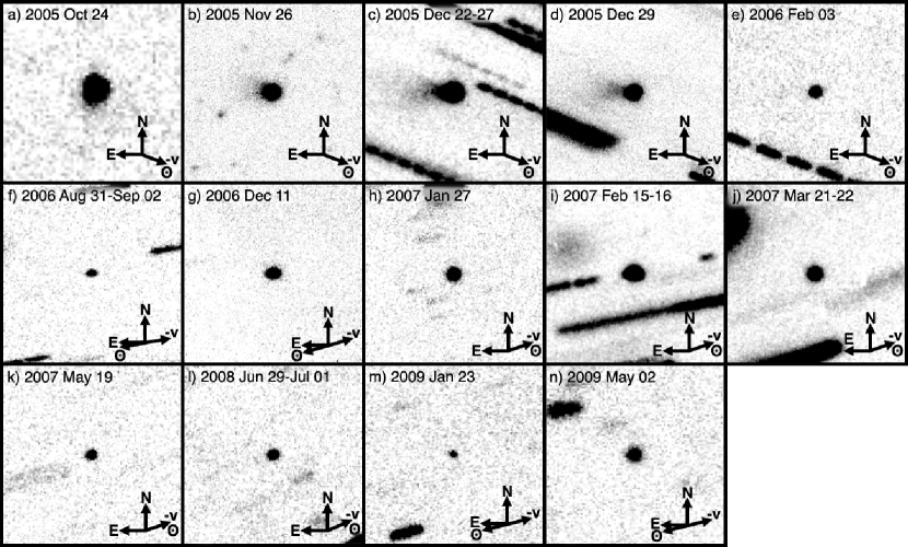
Figure 1: Composite images of 176P from $R$-band images taken during observations detailed in Table 1. Each image is $0\farcm 5\times 0\farcm 5$ with 176P at the centre, with arrows indicating north (N), east (E), the negative heliocentric velocity vector ($-v$), and the direction towards the Sun ($\odot$). Images shown comprise (a) 3000 s of exposure time on the Lulin 1.0 m telescope, (b) 240 s on the 8 m Gemini North telescope, (c) 37500 s on the University of Hawaii 2.2 m telescope, (d) 2520 s on Gemini North, (e) 3600 s on the UH 2.2 m, (f) 2400 s on the UH 2.2 m, (g) 9000 s on the UH 2.2 m, (h) 240 s on the 10 m Keck I telescope, (i) 24600 s on the UH 2.2 m, (j) 25800 s on the UH 2.2 m, (k) 3000 s on the UH 2.2 m, (l) 1440 s on the 3.54 m New Technology Telescope, (m) 240 s on the 4.2 m William Herschel Telescope, and (n) 600 s on the 2.5 m Isaac Newton Telescope.

For all nights on which 176P was observed, we combine individual $R$- or $r^{\prime}$-band images (aligned on the object’s photocenter) into deep composite images to assess the level of cometary activity present (Fig. 1). Activity is unambiguously detected in observations made of the object between UT 2005 November 26 and 2005 December 29. In these observations, no coma is apparent, though a fan-shaped tail is clearly visible. No activity in the form of a coma or tail is seen in the next available set of observations obtained on 2006 February 03 nor in any monitoring observations made since that time.

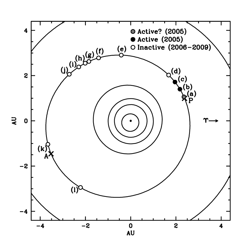
Figure 2: Orbital positon plot of active and inactive phases of 176P detailed in Table 1. The Sun is shown at the center as a solid dot, with the orbits of Mercury, Venus, Earth, Mars, 176P, and Jupiter (from the centre of the plot outwards) are shown as black lines. Solid circles mark positions where 176P was observed to be active, while open circles mark positions where 176P was observed to be inactive. Perihelion (P) and aphelion (A) positions are also marked with crosses. References: (a) 2005 Oct 24 (Hsieh, 2009), (b) 2005 Nov 26 (Hsieh & Jewitt, 2006); (c) 2005 Dec 22-29 (Hsieh & Jewitt, 2006); (d) 2006 Feb 03-08; (e) 2006 Aug 31 - Sep 02; (f) 2006 Dec 11-18; (g) 2007 Jan 27; (h) 2007 Feb 15-16; (i) 2007 Mar 21-22; (j) 2007 May 19; (k) 2008 Jun 29 - Jul 01; (l) 2009 May 03, where (d)-(l) are from this work.

Poor seeing during a precovery observation of 176P on 2005 October 24, just one month prior to the first confirmed observations of activity, prevents conclusive determination of the object’s active nature at the time. Photometric evidence (below), however, now suggests that the object may have in fact been active. Overall, 176P’s behavior is consistent with that of an object that exhibits activity near perihelion but not at other points in its orbit (Fig. 2). In all observations when 176P is observed to be active, the tail is directed approximately due east, roughly 20^∘ south of the anti-solar direction.

We also measure $BVRI$ colors of 176P on several occasions during its 2005 active period (Table 2), finding mean values of $B-V=0.63\pm 0.02$, $V-R=0.35\pm 0.02$, and $R-I=0.31\pm 0.04$, and no evidence of substantial variability. This lack of variability is unsurprising because, while no significant coma is observed, 176P may very well possess an unresolved coma (cf. 133P; Hsieh et al., 2010). If unresolved coma is present, not only will that coma not exhibit color variability as the nucleus rotates, it will also dampen any color variability that the underlying nucleus itself might exhibit.

3.2 Phase Function

Characterization of an object’s photometric dependence on changing solar phase angle, i.e., its phase function, permits data obtained at different observing geometries to be compared and combined, while also giving insight as to the properties of the surface material of the object itself (e.g., Bowell et al., 1989). To compute 176P’s phase function, we first consider only photometric data obtained when 176P appears to be inactive (i.e., from 2006 Feb 03 onwards; Table 1).

On several nights, a significant length of time ($\gtrsim 0.6$ hr) elapses from the time of our first observation of the object to the time of the last observation, during which the object could potentially undergo significant rotation. We refer to these data as “lightcurve observations” (Table 3). Observations on other nights that do not span a significant amount of time are referred to as “snapshot observations”. While on no occasion is 176P seen to reach both the maximum and minimum of its rotational lightcurve in a single night of observations, we can nevertheless exploit these lightcurve observations to obtain useful information regarding the midpoints of the rotational lightcurve on each night.

For computing 176P’s phase function, we aim to use its mean brightness (averaged over a full rotation) as a common reference point for data from different epochs. It is obviously not possible to know a priori the rotational phase of the object at the time of a given snapshot observation. As such, in using photometry from snapshot observations to compute 176P’s phase function, we assign a maximum uncertainty, $\sigma$, equal to half of the expected lightcurve range, $\Delta m$. This allows for the range of possible rotational phases up to and including the extreme case where the snapshot observation was obtained at either the object’s maximum or minimum brightness.

Unlike in snapshot observations, the rotational phase of lightcurve observations can be constrained by the observed brightness variation, $\delta m$, over the course of the observing period. If $\delta m\approx\Delta m$, the mean of the minimum and maximum brightness of the object during that set of lightcurve observations will be close to the midpoint of the actual lightcurve. We express these constraints by assigning uncertainties to the midpoints of our lightcurve observations equal to $\sigma=(\Delta m-\delta m)/2$. The final uncertainties listed in Table 3 reflect both these assigned uncertainties and the uncertainties in the computed mean brightnesses themselves.

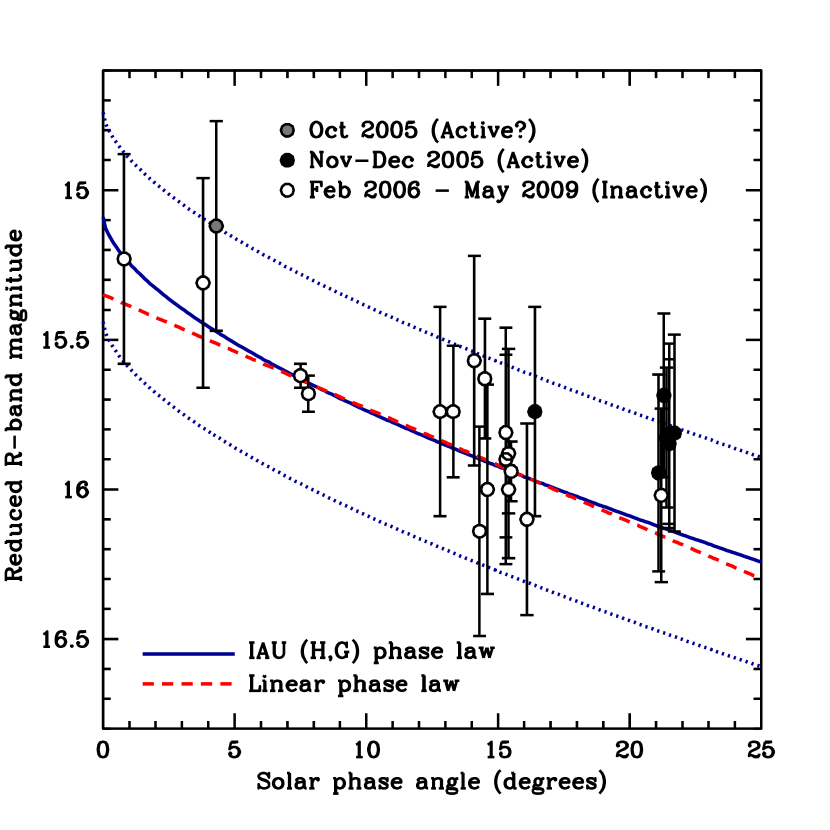
Figure 3: Phase functions for 176P. Points are estimated $R$-band magnitudes (normalized to heliocentric and geocentric distances of 1 AU; tabulated in Table 1) at the mid-point of the full photometric range of the nucleus’s rotational light curve. Solid circles denote photometry obtained while 176P was visibly active, while open circles denote photometry obtained while 176P appeared to be inactive. The dashed line represents a least-squares fit (excluding photometry points for which $\alpha<5^{\circ}$ where an opposition surge effect is expected) to a linear phase function where $m_{R}(1,1,0)=15.35\pm 0.08$ mag and $\beta=0.038\pm 0.008$ mag deg⁻¹. The solid line represents an IAU ($H,G$) phase function fit where $H_{R}=15.09\pm 0.05$ mag and $G_{R}=0.15\pm 0.10$, while the dotted lines indicate the expected range of possible magnitude variations ($\sim 0.35$ mag) due to the object’s rotation.

We then perform weighted fits of photometric data obtained from both lightcurve observations and snapshot observations to the IAU $H,G$ phase function (Bowell et al., 1989), finding best-fit parameters of $H=15.10\pm 0.05$ mag and $G=0.15\pm 0.10$, which are in agreement with the parameters calculated in Hsieh et al. (2009a) with fewer data points and a less sophisticated weighting scheme. We also fit our data to a linear phase function, omitting data points obtained at solar phase angles of $\alpha\lesssim 5^{\circ}$ at which opposition surge effects are expected, finding best-fit parameters of $m(1,1,0)=15.35\pm 0.05$ mag and $\beta=0.038\pm 0.005$, again in agreement with Hsieh et al. (2009a). These solutions and the data used to compute them are plotted in Figure 3.

For all of these calculations, we use $\Delta m=0.70$ mag based on the maximum photometric variation observed in lightcurve observations (Table 3). We note, however, that our eventual best-fit phase function parameters are not highly sensitive to the value chosen for $\Delta m$ as long as relative uncertainties for snapshot and lightcurve observations are preserved.

3.3 Photometric Confirmation of Activity

Once a phase function has been computed for 176P using inactive data, we can overlay photometric data for 176P obtained when the object was active. These data are plotted as solid circles in Figure 3 and can be seen to be consistently brighter than the expected mean brightness of the object at those phase angles, confirming the presence of excess flux attributable to cometary activity. This type of photometric detection of activity led to the discovery of activity in 95P/Chiron (Bus et al., 1988; Tholen et al., 1988; Meech & Belton, 1989; Hartmann et al., 1990) and was also used to detect unresolved coma for 133P (Hsieh et al., 2010) and to confirm the reactivation of 238P (Hsieh et al., 2011).

For data taken when 176P was seen to be visibly active (2005 November 26 to 2005 December 29), we find that the nucleus is, on average, $0.3\pm 0.1$ mag brighter than expected, given the $H$ and $G$ phase function parameters we derive in §3.2. Following Hsieh et al. (2010), we assume that the discrepancy between the observed magnitude, $m_{obs}$, and the expected magnitude, $m_{exp}$, is due to dust contamination, and that the albedos of the nucleus and dust are equal. We then calculate that the scattering surface area of the dust coma (and any portion of the tail also contained within the photometry aperture), $A_{d}$, is $\sim 30$% that of the inactive nucleus, $A_{n}$, using

$${A_{d}\over A_{n}}=10^{0.4(m_{exp}-m_{obs})}-1.$$ (1)

Using $A_{n}=\pi r_{e}^{2}=(1.3\pm 0.2)\times 10^{7}$ m², where $r_{e}=2.0\pm 0.2$ km is the effective radius of 176P’s nucleus (Hsieh et al., 2009a), we therefore find $A_{d}=(0.4\pm 0.2)\times 10^{7}$ m². Assuming a typical dust grain radius of 10 $\mu$m — similar to dust grain radii found for 133P (Hsieh et al., 2004) and consistent with dust modeling results for 176P (§4) — and a bulk grain density of $\rho_{d}=1300$ kg m^-3 (Hsieh et al., 2004), we find an approximate total coma dust mass of $M_{d}\sim(7.0\pm 3.5)\times 10^{4}$ kg, comparable to coma dust masses found for 133P (cf. Hsieh et al., 2010).

3.4 Rotation

3.4.1 Period Determination

Given the minimal nucleus-obscuring coma observed during 176P’s 2005 active phase, we performed phase dispersion minimization analysis (e.g., Stellingwerf, 1978) on the photometry data we obtained during that time in an attempt to ascertain the nucleus’s synodic rotation period, but were unable to identify a period that would allow us to produce a convincing lightcurve. At the time, we attributed this failure to find a plausible rotation period to a probable extremely slow rotation rate, which made it difficult to sample a significant portion of the rotational lightcurve in a single night (where the object was visible for $\sim$4 hr in 2005 December), and possible aliasing caused by a rotation period close to the Earth’s own daily 24-hr rotation period.

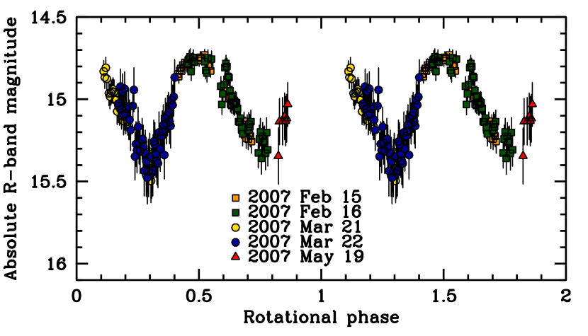
Figure 4: Phase-angle-normalized, reduced-magnitude data (i.e., normalized to $\alpha=0^{\circ}$ and $R=\Delta=1$ AU) for observations of 176P/LINEAR made between 2007 February and May, phased to a rotation period of $P_{rot}=22.23$ hr.

A more suitable data set for determining 176P’s rotation period was obtained on two nights in 2007 February and two additional nights in 2007 March. In addition to affording longer nightly visibility windows ($\sim$7 hr in February and $\sim$5 hr in March), the timing of the observations over two consecutive months allowed us to avoid both aliasing effects and complications due to significant changes in viewing geometry. Applying the same phase dispersion minimization techniques as before and phasing our data to candidate rotation periods to assess plausibility, we find a likely rotation period of $P_{rot}=22.23\pm 0.01$ hr (assuming the lightcurve is double-peaked) and a peak-to-trough photometric range of $\Delta m\sim 0.7$ mag (Fig. 4; where data for 2007 May 19 is overplotted to check for consistency). We estimate the uncertainty on the period by slowly varying the optimum period and re-phasing the data until we determine that the lightcurve is noticeably out of phase. We also find possible but less likely candidate periods of $P_{rot}=22.57$ hr, $P_{rot}=22.83$ hr, and $P_{rot}=23.20$ hr, all of which produce lightcurves with larger phase dispersions than for $P_{rot}=22.23$ hr.

The lightcurve we find using our most likely rotation period is incompletely sampled, but otherwise appears convincing. These results confirm our preliminary findings from the analysis of our 2005 data that the rotation of the object is extremely slow, but also show that the object is relatively elongated, with an axis ratio of $a/b>10^{0.4\Delta m}$, or $a/b>1.9$. Interestingly, the lightcurve also exhibits features such as a V-shaped minimum and an inverted U-shaped maximum that are qualitatively like those of contact binaries (e.g., Sheppard & Jewitt, 2004; Mann et al., 2007; Lacerda, 2008), though the photometric range we observe for 176P is not quite as large as is normally expected for such systems ($\Delta m>0.9$ mag; Lacerda, 2008).

3.4.2 2005 Photometry Revisited

Having achieved a reasonable lightcurve using 2007 data (§3.4), we turn back to our 2005 data and attempt to phase them using the same rotation period (Fig. 5). When phased together, the data fit together far less well than the 2007 data, but the resemblance to the 2007 lightcurve is clear. We attribute much of the scatter in the data to the extreme sensitivity of photometry of active objects to seeing, where even small changes in image quality from exposure to exposure can cause significantly different amounts of dust contamination to be present in each photometry aperture. We believe this effect to be the cause of the slight brightness excess toward the second half of our 2005 December 25 observations (Fig. 5). On 2005 December 24, we find an overall brightness excess for the comet in the range of $\sim 0.1-0.2$ mag (see Table 1), but given that the comet was passing through a particularly dense star field on this night, we attribute this excess to contamination from unseen faint field stars, and omit this data from Figure 5 for clarity. An active cometary object may of course be expected to occasionally exhibit short-lived outbursts, but given the random (non-correlated with rotational phase) and short-lived nature of the observed photometric anomalies, we find that they are adequately explained by fluctuations in the nightly seeing and, on occasion, by faint field star contamination.

Significantly, the phased 2005 data appear to exhibit a far smaller photometric range than the 2007 data, showing a peak-to-trough variation of $\Delta m\sim 0.2$ mag, down from $\Delta m\sim 0.7$ mag in 2007. As the observed photometric range of a rotating nucleus can be damped by a superimposed coma of constant brightness (determined to be present for 176P in §3.3), before evaluating the physical implications of this change in observed photometric range, we must first determine how much of this effect could be due to coma damping.

Noting that the measured flux from an active comet, $F_{obs}$, consists of the sum of the fluxes from the nucleus and dust contained within the photometry aperture, we can write

$$10^{0.4\Delta m_{obs}}={F_{obs,max}\over F_{obs,min}}=\left({F_{n,max}+F_{d}\over F_{n,min}+F_{d}}\right)$$ (2)

where $\Delta m_{obs}$ is the observed photometric range of the lightcurve, $F_{obs,max}$ and $F_{obs,min}$ are the maximum and minimum fluxes, respectively, observed for the active nucleus, $F_{n,max}$ and $F_{n,min}$ are the maximum and minimum fluxes, respectively, for which the nucleus is responsible, and the flux due to dust, $F_{d}$, is assumed to be constant.

For a true nucleus axis ratio (i.e., uncontaminated by coma) of $(a/b)_{n}$, nucleus fluxes can be expressed as follows:

$$F_{n,max}=\left({a\over b}\right)_{n}^{1/2}F_{n}$$ (3)

and

$$F_{n,min}=\left({a\over b}\right)_{n}^{-1/2}F_{n}$$ (4)

where $F_{n}$ is the average flux of the nucleus over one full rotation.

Then, substituting Equations 3 and 4 into Equation 2, we find

$$\left({a\over b}\right)_{n}+\left[{F_{d}\over F_{n}}\left({1-10^{0.4\Delta m_{obs}}}\right)\right]\left({a\over b}\right)_{n}^{1/2}-10^{0.4\Delta m_{obs}}=0$$ (5)

which can then be solved for $(a/b)_{n}^{1/2}$ using standard techniques for solving quadratic polynomials, where $F_{d}/F_{n}=A_{d}/A_{n}$ is given by Equation 1. Taking the positive root of Equation 5 (since Equations 3 and 4 must produce positive values), we find $(a/b)_{n}=1.27$, meaning that even accounting for coma contamination, the photometric range of the bare nucleus in 2005 is $\Delta m_{n}=0.26$, still much smaller than that observed in 2007.

3.4.3 Implications for Pole Orientation and Physical Nature

The plausibility of the seasonal heating hypothesis as a mechanism for modulating MBC activity (first proposed for 133P; Hsieh et al., 2004), depends crucially on each object having a pole orientation compatible with its activity profile. Pole orientations are currently unknown for all MBCs, though some constraints placed on 133P’s pole orientation by Tóth (2006) are thus far consistent with seasonal modulation of that MBC’s activity.

In the case of 176P, we can use the rotational lightcurves shown in Figures 4 and 5 to place constraints on its pole orientation. These figures show that the photometric range of 176P’s lightcurve changed appreciably between 2005 ($\Delta m\sim 0.2$ mag) and 2007 ($\Delta m\sim 0.7$ mag), which suggests that the object has significant obliquity. The available data (incomplete lightcurves at two epochs) are not sufficient to uniquely determine the spin pole direction of 176P. For example, we are unable to break the degeneracy between north and south pole. However, we can still use those data to obtain useful constraints on the rotational pole of 176P.

In particular, we are interested in constraining the shape and obliquity of 176P and verifying if the data are consistent with the seasonal hypothesis for MBC activity. According to the seasonal hypothesis, 176P should have non-zero obliquity and be active close to one of its solstices. We thus elect to parameterize the orientation of the spin pole of 176P by its obliquity, $\varepsilon$, and by the true anomaly of the solstice, $\nu_{0}$, which we assume to be the northern hemisphere summer solstice. For instance, if 176P were at solstice exactly at perihelion, then $\nu_{0}=0$°. We assume the already low orbital inclination ($i=0.23$°) of 176P to be exactly zero for the purpose of this analysis.

To investigate the lightcurve behavior of 176P we employ the simulations described in Lacerda & Jewitt (2007). These simulations place triaxial ellipsoids (semi-axes $a\geq b\geq c$) at pre-selected illumination and viewing angles and register the integrated reflected flux as a function of rotational phase (assuming simple principal axis rotation about the ellipsoids’ short axes) to extract modeled lightcurves. In addition to observing geometry (completely defined by $\varepsilon$, $\nu_{0}$, and the phase angle $\alpha$), the model takes as parameters the axis ratios ($0<c/a\leq b/a\leq 1$) of the triaxial ellipsoid and the scattering law. For simplicity, we use prolate ellipsoids ($c/a=b/a$) and a Lommel-Seeliger “lunar” scattering function which has no free parameters and is appropriate for simulating the low albedo ($p_{R}=0.06\pm 0.02$; Hsieh et al., 2009a) surface of 176P. In what follows, we compare the model lightcurves with the data (Figs. 4 and 5) from 2005 (chiefly taken at point (c) in Fig. 2) and 2007 (taken at points (h), (i) and (j) in Fig. 2).

Due to the underconstrained nature of this problem given the available data, we only consider two limiting scenarios, one in which we simply assume that the lightcurve amplitude observed in 2007 represents the object’s maximum range, placing it at equinox during those observations, and a second scenario that is physically motivated where we assume that the object was receiving maximal heating at the time when our 2005 observations showed it to be active, placing solstice at perihelion.

First, we consider the possibility that 176P was close to equinox during the 2007 measurements, implying that the solstice occurs around true anomaly $\nu_{0}=21$°, i.e., just after the 2005 observations. In that case we can use the photometric range in 2007 to obtain a direct estimate of the $b/a$ axis ratio from the relation $\Delta m=-2.5\log(b/a)$. Using $\Delta m\sim 0.7$ mag, we find $b/a\sim 0.52$.

Figure 6 (left panel) shows the 2007 lightcurve data overplotted on three simulations spanning $0.54\leq b/a\leq 0.58$. The reason why the best-fit model shapes are slightly less elongated than the purely geometric estimate, $b/a=0.52$, is that limb darkening effects contribute to increase the photometric variability beyond the geometric expectation. Each model was calculated using the mean phase angle and true anomaly of the 2007 observations. Under these conditions, the obliquity is approximately determined by the 2005 “solstice” data. An obliquity of $\varepsilon=0$° would result in a nearly constant photometric range throughout the orbit, whereas $\varepsilon=90$° would imply negligible photometric variation in 2005. We find that an obliquity $\varepsilon\sim 60$° for an object with an axis ratio $b/a\sim 0.56\pm 0.03$ fits the 2005 data well (Fig. 6, right panel).

We now consider a second scenario in which solstice occurs at perihelion, $\nu_{0}=0$°, just before the period of activity in 2005. We reason that if the activity is powered by the seasonal heating of sub-surface ice, then it should begin at or shortly after the time of maximum localized heating, i.e., the solstice. If $\nu_{0}=0$°, then equinox takes place at true anomaly $\nu=90$°, or about 20° before the 2007 data were taken. In this scenario, 176P must be more elongated than determined above. In Figure 7 we show this to be the case: to simultaneously fit the 2005 and 2007 data, for an obliquity of $\varepsilon=60$°, an axis ratio $b/a\sim 0.52$ is required.

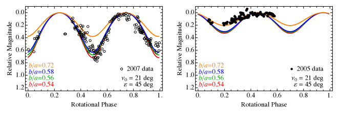
Figure 8: Same as Fig. 6 but for obliquity $\varepsilon=45$°and an ellipsoid with axis ratio $b/a=0.72$ (solid orange line).

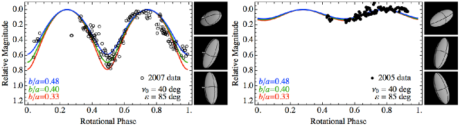
Figure 9: Same as Fig. 6 but for obliquity $\varepsilon=85$°, solstice position $\nu_{0}=40$° and ellipsoids with axis ratios $b/a=0.33$ (red), $b/a=0.40$ (green), and $b/a=0.48$ (blue).

In both scenarios, we note that models using significantly smaller obliquities (e.g., $\varepsilon=45$°) cannot simultaneously fit the 2005 and 2007 (e.g., Fig. 8). Higher obliquities are possible, but require a more elongated nucleus shape for 176P and a later solstice location along the orbit. Figure 9 shows the result of simulations for solstice at $\nu_{0}=40$°, obliquity $\varepsilon=85$°, and shapes $0.33\leq b/a\leq 0.48$. However, objects with such extreme axis ratios (3:1, 2.5:1 and 2.1:1 in Fig. 9) are hydrostatically unstable (Jeans, 1919) and require significant material strength to retain their shape. Alternatively, such extreme configurations may be explained by contact binaries (Lacerda & Jewitt, 2007), but our current data set is insufficient for confirming or ruling out this possibility. Solstice positions significantly outside the interval $0\arcdeg\leq\nu_{0}\leq 40\arcdeg$ (or equivalently, $180\arcdeg\leq\nu_{0}\leq 220\arcdeg$, due to the fact that “summer” and “winter” solstices are indistinguishable in this analysis) are untenable as the 2005 data with its smaller $\Delta m$ would fall as close or closer to the equinox than the 2007 data with its larger $\Delta m$, when in fact $\Delta m$ should reach a maximum at equinox.

In conclusion, our data strongly suggest that 176P is highly elongated, close to a 2:1 axis ratio, and has significant obliquity, close to $\varepsilon=60$°. The solstice positions that best fit the data are located close to the active portion of the orbit, around $\nu_{0}=20\pm 20$°, placing the other solstice at $\nu_{180}=200\pm 20$°, and equinoxes at $\nu_{90}=110\pm 20$°and $\nu_{270}=290\pm 20$°. These constraints on the obliquity and solstice position of 176P are consistent with the seasonal hypothesis to explain the activity of MBCs.

4 DUST MODELING

In order to place quantitative constraints on 176P’s dust emission, we generate a series of numerical models for the dust and attempt to match them to our observations. Due to the limited observational data available and the resulting underconstrained nature of this dust modeling effort, we recognize from the outset that it will not be possible to achieve an exact model of 176P’s activity. As such, we purposefully formulate our modeling strategy to simply achieve constraints on particular key properties such as grain sizes, ejection velocities, and the temporal behavior of the dust emission.

Standard dust modeling (e.g., Finson & Probstein, 1968) typically makes use of syndyne curves, which are lines representing the positions of particles of constant sizes ejected at different times where ejection velocities are assumed to be zero, and synchrone curves, which are lines representing the positions of particles of different sizes ejected at the same time with zero velocity. In the case of 176P, an extremely low inclination means that all synchrone and syndyne curves actually overlap with one another in the object’s orbit plane, making it very difficult to use this type of analysis to study 176P’s dust emission. We note, however, that the orientation of 176P’s dust tail does not coincide with its orbit plane, and thus, does not actually coincide with any syndyne or synchrone curves (Fig. 1b,c,d), and therefore we must consider asymmetric dust emission (as in a jet), similar to that considered in our previous analysis of 238P (Hsieh et al., 2009b). The methods used in the following analysis are the same as those used in that previous work except where otherwise specified.

Assuming jet-driven dust emission, we assume that the central axis of the cone points in a particular direction in the inertial frame (i.e., toward right ascension $\alpha_{jet}$, and declination $\delta_{jet}$). For a rotating body and a non-equatorial jet, it should be noted that the effective time-averaged jet position in this model actually simply corresponds to the nearest rotational pole, where the derived jet width will be somewhat larger than the actual jet width due to the sweeping motion caused by the body’s rotation (cf. Fig. 10). For simplicity, we assume that Earth-bound observers are situated outside the cone defined by the rotating jet, and that the strength of the jet does not vary with rotational phase.

The time-averaged jet is presumed to originate at the subsolar point and have a half-opening angle of $w=45$°. We furthermore assume that dust particles are released homogeneously from a spherical body and that emission only occurs on the day-time side of the body. Dust particle sizes are parameterized in standard fashion where $\beta$ denotes the ratio of a particle’s acceleration due to solar radiation pressure to its acceleration due to gravity. Terminal velocities, $v_{ej}$, of ejected dust particles are given by

$$v_{ej}(r_{h},\beta)=v_{0}\beta^{u_{1}}\left({r_{h}\over{\rm AU}}\right)^{-u_{2}}$$ (6)

where $r_{h}$ is the heliocentric distance, $v_{0}$ is the reference ejection velocity in m s^-1 (assumed here to be $v_{0}=25$ m s^-1 based on our work with 238P; Hsieh et al., 2009b) of particles with $\beta=1$ at $r_{h}=1$ AU, and $u_{1}$ and $u_{2}$ (assumed here to be $u_{1}=u_{2}=0.50$) are the power indices of the reference ejection velocity dependence on $\beta$ and $r_{h}$. We use an exponential size distribution with an index of $q=-3.5$, minimum $\beta$ value of $\beta_{min}=9\times 10^{-2}$, and maximum $\beta$ value of $\beta_{max}=10^{-1}$, and an exponential dust production rate dependence on heliocentric distance with an index of $k=3$. Dust emission is assumed to begin 1 year prior to perihelion passage and is terminated on 2006 January 1 (three days after 176P was last observed to be active). We assume such an early start date to allow time for the dust to evolve to a “steady” state, but given the short dissipation timescales for micron-scale dust particles, also note that most of the dust that is actually observed is likely to have been ejected far more recently.

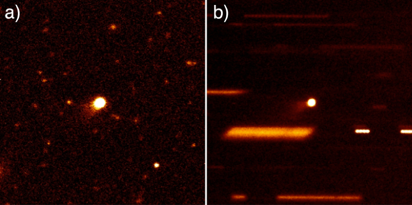
Figure 11: Observations of 176P (obtained with Gemini North on (a) 2005 Nov 26 and (b) 2005 Dec 29) used to constrain numerical models (§4), where images are shown in the ecliptic coordinate system such that the orbital plane of 176P is effectively horizontal and where radiation pressure pushes dust particles to the left.

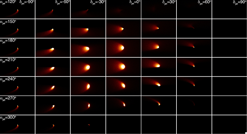
Figure 12: Images of dust ejection models for 2005 Nov 26 for $10^{-3}<\beta<10^{-1}$ and different jet directions as labeled, where $\alpha_{\rm jet}$ is constant for each row of models and $\delta_{\rm jet}$ is constant for each column of models. In all panels, the source of emission (i.e., the nucleus) is at the center of each image.

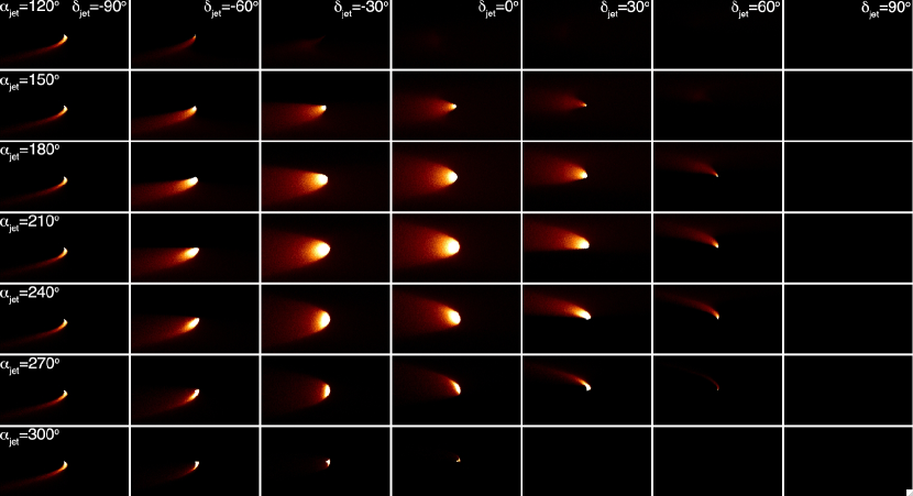
Figure 13: Images of dust ejection models for 2005 Dec 29 for $10^{-3}<\beta<10^{-1}$ and different jet directions as labeled, where $\alpha_{\rm jet}$ is constant for each row of models and $\delta_{\rm jet}$ is constant for each column of models. In all panels, the source of emission (i.e., the nucleus) is at the center of each image.

We show resulting modeled dust clouds for 2005 November 26 and 2005 December 29 for different jet orientations in Figures 12 and 13, respectively. Comparing these to the observations in Figure 11, we see that reasonable matches to our data are provided by models with jet directions of $180\arcdeg\lesssim\alpha_{\rm jet}\lesssim 120$°and $\delta_{\rm jet}\approx-60$°, or approximately oriented towards the Sun during the comet’s active period. Crucially, all model scenarios also reproduce the non-detection of activity on 2006 February 03 (Fig. 1), where all dust particles in each scenario have dispersed from the field of view by that time. This rapid disappearance of dust activity did not occur from a previous set of test scenarios for which we assumed much larger particles were present ($\beta_{min}=10^{-3}$). We thus conclude that the dust particles ejected by 176P must have been on the order of $\sim$10 $\mu$m in size (corresponding to $\beta\sim 10^{-1}$), similar to the dominant particle sizes found for 133P (Hsieh et al., 2004). Using Equation 6, we find an approximate ejection velocity for these particles of $v_{ej}\sim 5$ m s^-1, or somewhat faster than the $v_{ej}\sim 1$ m s^-1 ejection velocities found for 133P.

To determine an approximate dust production rate, we refer back to our estimate for 176P’s unresolved coma mass in §3.3 of $M_{d}\sim 7\times 10^{4}$ kg. This mass estimate is based on nucleus photometry employing $3\farcs 0$-radius photometry apertures, which at the distance of 176P in December 2005, correspond to physical radii of $r_{coma}\approx 5000$ km. The time that it would take a dust particle to cross the photometry aperture can then be estimated as $t_{cross}=r_{coma}/v_{ej}\sim 1\times 10^{6}$ s, or about 12 days. Using this as the approximate timescale on which dust in the coma must be replaced by new dust production from the nucleus, we therefore find an approximate dust production rate of $dM/dt\approx M_{d}/t_{cross}\sim 0.07$ kg s^-1. This production rate is similar to that found for 133P by (Hsieh et al., 2004), but is also likewise probably accurate, at best, to an order of magnitude.

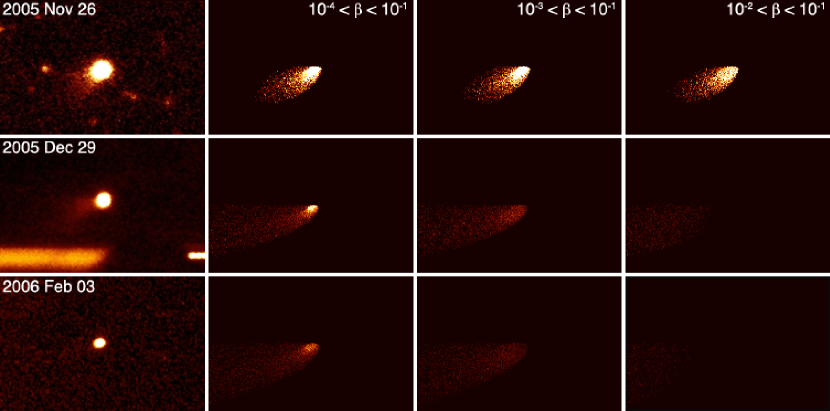
Figure 14: Comparison of observations (first column of panels) with images of impulsive dust ejection models using different particle size distributions ($10^{-4}<\beta<10^{-1}$ in the second column, $10^{-3}<\beta<10^{-1}$ in the third column, and $10^{-2}<\beta<10^{-1}$ in the fourth column). Data and models for 2005 November 26, 2005 December 29, and 2006 February 03 are shown along the first, second, and third rows, respectively. All models consist of dust ejected on a single day on November 15 (four weeks after perihelion and 11 days before cometary activity was first observed on November 26). In all panels, the source of emission (i.e., the nucleus) is at the center of each image.

We are further interested in whether 176P’s dust emission is only consistent with continuous emission, i.e., that would be expected if the activity is driven by the sublimation of ice, or whether it can also be reproduced by an impulsive emission event, i.e., if 176P’s dust tail solely consists of ejecta produced in an impact by another asteroid. To test this, we produce another series of models in which dust emission is limited to a single burst of particles. We test three different size distributions — $10^{-4}<\beta<10^{-1}$, $10^{-3}<\beta<10^{-1}$, $10^{-2}<\beta<10^{-1}$ — where dust in each model is ejected on a single day (2005 November 15), which is four weeks after perihelion and 11 days before activity was first observed (Fig. 14). We then continue to follow the evolution of the dust and compare its appearance in each model to observations on 2005 December 29 and 2006 February 03.

We clearly see that for the models including large particles ($\beta_{min}=10^{-4}$ and $\beta_{min}=10^{-3}$; second and third columns of Fig. 14), the appearance of the comet remains approximately constant between November and December, as is observed. However, the comet retains its appearance through February as well (consistent with our continuous emission models), which is inconsistent with observations. If only smaller particles are included ($\beta_{min}=10^{-2}$; fourth column of Fig. 14), we note that the dust cloud does dissipate appreciably by February, but also undergoes significant dissipation by December, inconsistent with observations. Thus, we find that a single burst of particles cannot produce a dust cloud that simultaneously remains constant between 2005 November 26 and 2005 December 29, but then dissipates by 2006 February 03.

We therefore conclude that 176P’s activity is most likely driven by an extended emission event, in which 176P’s dust tail is continuously replenished by small, fast-dissipating particles between 2005 November and December, allowing it to maintain its appearance, but where dust emission ceases sometime in December, leading to the nearly complete dissipation of the dust cloud by the time the comet is observed again on 2006 February 03. This behavior strongly suggests that 176P’s activity is driven by the sublimation of volatile ices, as was previously found for fellow MBCs, 133P and 238P (Hsieh et al., 2004, 2009b). If this conclusion is correct, we would also expect 176P to exhibit repeated activity, similar to 133P and 238P (Hsieh et al., 2010; Hsieh, 2010), perhaps during its upcoming perihelion passage (2011 July 01). Observations of renewed activity at this time will provide strong support for sublimation at the cause of 176P’s activity. Conversely, however, if no activity is observed, reconsideration of impact-generated dust emission as the source of 176P’s activity may be necessary.

In terms of pole orientation, our dust modeling analysis is remarkably consistent with the results of our lightcurve analysis (§3.4.3), as a jet orientation of $180\arcdeg\lesssim\alpha_{\rm jet}\lesssim 120\arcdeg$ and $\delta_{\rm jet}\approx-60\arcdeg$ that is effectively coincident with the object’s rotational pole corresponds to an orbital obliquity of $50\arcdeg\lesssim\varepsilon\lesssim 75\arcdeg$. The consistency of these results is encouraging support for their accuracy, and strongly suggests that 176P is in fact a high-obliquity object that is at solstice around the time that a localized site in the “summer-time” hemisphere experiences active sublimation, just as described under the seasonal heating hypothesis for MBCs.

5 DISCUSSION

5.1 Activity Profile

Little is currently known about the activity profile of 176P. During 176P’s 2005 active period, dust emission appeared to end between $\nu\sim 19\arcdeg$ and $\nu\sim 28\arcdeg$ in true anomaly. No conclusive evidence of activity was observed from Lulin Observatory when the comet was at a true anomaly of $\nu=1.4\arcdeg$, though a photometric analysis (§3.3) suggests that activity may have been present but simply escaped detection, perhaps due to poor seeing. As such, the point at which 176P’s activity began is essentially unconstrained. If 176P is similar to 133P and exhibits recurrent, seasonally-modulated dust emission that persists over $\sim 90\arcdeg$ of its orbit, though, we might have expected it to resume cometary activity as early as 2010 September when it reached $\nu\sim 290\arcdeg$. If, however, 176P is active over a much smaller portion of its orbit than 133P (as it might, for example, if shadowing due to local topography also has a strong activity-modulating effect), then activity may not return until closer to the object’s perihelion passage on 2011 July 01. Continued monitoring of 176P is highly encouraged to help clarify this issue.

5.2 Comparison to other MBCs

The activity of 176P is similar to 133P (Hsieh et al., 2004, 2010) in terms of dust output (c.f. §4), but much weaker than highly active MBCs like 238P (Hsieh et al., 2009b, 2011), P/2008 R1 (Garradd) (hereafter P/Garradd; Jewitt et al., 2009), or P/2010 R2 (La Sagra) (hereafter P/La Sagra). Recently observed comet-like activity for two other objects in the main asteroid belt — P/2010 A2 (LINEAR) and (596) Scheila (Birtwhistle et al., 2010; Larson, 2010) — is likely to be due to impact-generated ejecta clouds, and not sublimation-driven dust emission (Jewitt et al., 2010; Snodgrass et al., 2010; Jehin et al., 2011), and so we omit these so-called “disrupted asteroids” from this discussion.

Differences in MBC activity strength could be due to low-activity MBCs actually being intrinsically less icy than highly active MBCs, or perhaps simply activated less recently than highly active MBCs, resulting in greater depletion of their current active sites. Observations of highly active MBCs during successive future active periods to track their decline in strength, if any, will help to clarify this issue. Noting the distribution of activity levels of MBCs discovered in the future may also be informative. A high ratio of low-activity objects to highly active objects could indicate asymptotic declines in activity strength as individual active sites become depleted. On the other hand, a flatter distribution of MBCs of varying strengths, or evidence that activity strength has a particular spatial dependence, could indicate that activity strength is more strongly dependent on the intrinsic ice content of each body (and by extension, the ice content of the surrounding population). Any analysis of this nature will also have to account for observational discovery biases towards more highly active objects.

The activity profile discussed above (§5.1) is particularly interesting in relation to 133P in that while 133P becomes active shortly before perihelion, 176P becomes inactive shortly after perihelion (Fig. 2). This fact is significant because if 176P’s thermal inertia is low, it should reach its maximum overall temperature close to perihelion. If thermal inertia is high, 176P’s temperature may not be at its maximum at perihelion, but should instead be increasing at this point of close approach to the Sun. In either case, the fact that 176P’s activity ends (or at least declines below detectable levels) shortly after the object’s overall temperature has peaked or is even still increasing strongly favors a scenario in which activity is modulated by seasonal effects, as proposed for 133P (Hsieh et al., 2004, 2010), rather than proximity to the Sun and overall temperature.

One caveat, though, is that we do not actually know whether the duration of 176P’s activity is similar to 133P’s (i.e., persisting over $\sim$25% of its orbit). The active portion of 176P’s orbit might still be centered on perihelion if, in addition to ending just after perihelion, it also only starts just before perihelion, giving it a much shorter active arc than 133P. Such a shorter active arc could perhaps be due to a much smaller (or older and therefore more depleted) supply of exposed volatile material, or topography imparting much more local shadowing, and therefore a much sharper seasonal effect, than on 133P. Again, as discussed above, continued monitoring of the object in search of resumed activity as it approaches its next perihelion passage will be essential for resolving these questions.

6 SUMMARY

We present a physical analysis of main-belt comet 176P/LINEAR based on optical observations and numerical modeling, finding the following key results:

1. In optical imaging data obtained between late 2005 and mid-2009, we detect the presence of cometary activity for 176P between 2005 November 26 and 2005 December 29, and do not detect activity between 2006 February 03 and 2009 May 03, placing the apparent cessation point for 176P’s activity at 20^∘-25^∘ past perihelion. The turn-on point for activity remains unknown at this time.

2. Using photometric data obtained when no activity was detected for 176P, we find best-fit IAU phase function parameter values of $H=15.10\pm 0.05$ mag and $G=0.15\pm 0.10$, and best-fit linear phase function parameter values of $m(1,1,0)=15.35\pm 0.05$ mag and $\beta=0.038\pm 0.005$ mag deg^-1.

3. Using data obtained in 2007 when no activity was detected, we also find a rotation period solution of $P_{rot}=22.23\pm 0.01$ hr and a photometric range of $\Delta m\sim 0.7$ mag. Using this rotational period to phase data from 2005 when 176P was active, we find a much smaller photometric range of $\Delta m\sim 0.2$ mag which cannot be fully accounted for by coma contamination and as such is attributed by us to viewing geometry effects. From these lightcurve measurements, we derive a likely orbital obliquity of $\varepsilon\sim 60^{\circ}$ and an axis ratio of $1.8<b/a<2.1$.

4. In performing dust modeling of 176P’s activity, we noted that the orientation of the dust tail does not coincide with any syndyne or synchrone curves, requiring us to consider asymmetric dust emission, e.g., a cometary jet. We find plausible fits to our data using a continuous dust emission model with a particle size range of $9\times 10^{-2}<\beta<10^{-1}$ and a reference ejection velocity of $v_{0}=60$ m s^-1. Our data are not consistent with any impulsive dust emission scenarios that we investigated. We find a likely jet orientation (and therefore rotational pole orientation) of $180\arcdeg\lesssim\alpha_{\rm jet}\lesssim 120$°and $\delta_{jet}\approx-60^{\circ}$, in good agreement with our lightcurve analysis above.

Table 1: Observation Log

UT Date	Tel.	$N$	$t$	Filters	$\theta_{s}$	Active?	$\nu$	$R$	$\Delta$	$\alpha$	$\alpha_{pl}$	$m_{R}$	$m_{R}(1,1,\alpha)$
2005 Oct 18	Perihelion …………………………………………………..						0.0	2.58	1.59	1.5	–0.1	……………………………………..
2005 Oct 24	Lulin	10	3000	$R$	1.5	yes?	1.4	2.58	1.60	4.3	–0.1	18.20$\pm$0.01	15.12$\pm$0.01
2005 Nov 26	Gemini	2	240	$r^{\prime}$	0.6	yes	10.1	2.59	1.82	16.4	–0.1	19.11$\pm$0.04	15.74$\pm$0.04
2005 Dec 22	UH/Tek	7	2100	$R$	1.1	yes	16.8	2.60	2.12	21.1	–0.1	19.65$\pm$0.01	15.95$\pm$0.01
2005 Dec 24	UH/Tek	26	7800	$R$	1.0	yes	17.3	2.60	2.15	21.3	–0.1	19.46$\pm$0.01	15.73$\pm$0.01
2005 Dec 25	UH/Tek	33	9900	$BVRI$	0.9	yes	17.6	2.60	2.16	21.4	–0.1	19.62$\pm$0.01	15.88$\pm$0.01
2005 Dec 26	UH/Tek	31	9300	$BVRI$	1.0	yes	17.8	2.60	2.17	21.5	–0.1	19.62$\pm$0.01	15.86$\pm$0.01
2005 Dec 27	UH/Tek	29	8700	$R$	0.8	yes	18.1	2.60	2.19	21.5	–0.1	19.59$\pm$0.01	15.81$\pm$0.01
2005 Dec 29	Gemini	34	3060	$g^{\prime}r^{\prime}i^{\prime}z^{\prime}$	0.7	yes	18.6	2.60	2.21	21.7	–0.1	19.62$\pm$0.01	15.80$\pm$0.01
2006 Feb 03	UH/Tek	11	3300	$R$	1.1	no	27.7	2.63	2.71	21.2	0.0	20.25$\pm$0.01	15.98$\pm$0.01
2006 Aug 31	UH/Tek	2	600	$R$	0.8	no	75.1	2.93	3.55	14.3	0.0	21.23$\pm$0.08	16.14$\pm$0.08
2006 Sep 02	UH/Tek	2	600	$R$	0.9	no	75.5	2.94	3.53	14.6	0.0	21.09$\pm$0.05	16.00$\pm$0.05
2006 Dec 11	UH/Opt	30	9000	$R$	1.0	no	94.4	3.12	2.42	14.5	–0.1	20.01$\pm$0.01	15.62$\pm$0.01
2006 Dec 16	UH/Opt	11	3300	$R$	0.9	no	95.3	3.13	2.38	13.3	–0.1	20.13$\pm$0.01	15.77$\pm$0.01
2006 Dec 18	UH/Opt	3	900	$R$	1.3	no	95.6	3.14	2.36	12.8	–0.1	20.09$\pm$0.09	15.74$\pm$0.09
2007 Jan 27	Keck	3	240	$R$	0.9	no	102.5	3.21	2.23	0.8	–0.1	19.50$\pm$0.01	15.23$\pm$0.01
2007 Feb 15	UH/Tek	30	9000	$R$	0.9	no	105.6	3.25	2.33	7.5	0.0	19.87$\pm$0.01	15.47$\pm$0.01
2007 Feb 16	UH/Tek	49	14700	$R$	1.2	no	105.8	3.25	2.33	7.8	0.0	19.93$\pm$0.01	15.53$\pm$0.01
2007 Mar 21	UH/Tek	35	10500	$R$	0.8	no	111.1	3.31	2.72	15.4	0.0	20.71$\pm$0.01	15.94$\pm$0.01
2007 Mar 22	UH/Tek	51	15300	$R$	1.3	no	111.3	3.31	2.73	15.5	0.0	20.82$\pm$0.01	16.04$\pm$0.01
2007 May 19	UH/Tek	7	2100	$R$	1.1	no	120.2	3.41	3.64	16.1	0.1	21.57$\pm$0.05	16.10$\pm$0.05
2008 Jun 29	NTT	2	360	$R$	1.3	no	173.2	3.80	3.80	15.4	0.1	21.68$\pm$0.07	15.88$\pm$0.07
2008 Jun 30	NTT	3	540	$R$	1.0	no	173.3	3.80	3.81	15.3	0.1	21.70$\pm$0.05	15.90$\pm$0.05
2008 Jul 01	NTT	3	540	$R$	1.1	no	173.4	3.80	3.83	15.3	0.1	21.63$\pm$0.05	15.81$\pm$0.05
2008 Aug 25	Aphelion …………………………………………………….						180.0	3.81	4.52	9.9	0.0	……………………………………..
2009 Jan 23	WHT	4	240	$R$	0.8	no	198.0	3.77	4.01	14.1	0.0	21.47$\pm$0.10	15.57$\pm$0.10
2009 May 03	INT	2	600	$R$	1.8	no	210.5	3.69	2.70	3.8	0.1	20.30$\pm$0.04	15.31$\pm$0.04
2011 Jul 01	Perihelion …………………………………………………..						0.0	2.58	2.98	19.4	0.1	……………………………………..

Table 2: Color Measurements

UT Date	$B-V$	$V-R$	$R-I$
2005 Dec 25	0.61$\pm$0.03	0.32$\pm$0.02	0.27$\pm$0.03
2005 Dec 25	0.61$\pm$0.03	0.36$\pm$0.03	0.27$\pm$0.04
2005 Dec 26	0.64$\pm$0.03	0.37$\pm$0.02	0.35$\pm$0.03
2005 Dec 29	0.64$\pm$0.02	0.36$\pm$0.02	0.32$\pm$0.02
Mean	0.63$\pm$0.02	0.35$\pm$0.02	0.31$\pm$0.04

Table 3: Lightcurve Observations

UT Date	$\Delta t_{obs}$	Range	$m_{mid}$	$m_{mid}(1,1,\alpha)$
2006 Feb 03	1.65	0.13$\pm$0.06	20.28$\pm$0.06	16.02$\pm$0.29
2006 Dec 11	4.23	0.39$\pm$0.12	20.02$\pm$0.12	15.63$\pm$0.20
2006 Dec 16	1.98	0.28$\pm$0.05	20.10$\pm$0.05	15.74$\pm$0.22
2007 Feb 15	6.71	0.51$\pm$0.04	19.92$\pm$0.04	15.62$\pm$0.04
2007 Feb 16	7.34	0.55$\pm$0.06	20.01$\pm$0.06	15.68$\pm$0.06
2007 Mar 21	4.66	0.63$\pm$0.07	20.77$\pm$0.07	16.00$\pm$0.08
2007 Mar 22	5.12	0.55$\pm$0.10	20.83$\pm$0.10	16.05$\pm$0.13
2007 May 19	0.86	0.31$\pm$0.22	21.53$\pm$0.22	16.06$\pm$0.32

Figure 5: Phase-angle-normalized, reduced-magnitude data (i.e., normalized to $\alpha=0^{\circ}$ and $R=\Delta=1$ AU) for observations of 176P/LINEAR made between 2005 Dec 22 and 2005 Dec 29, phased to a rotation period of $P_{rot}=22.23$ hr.

Figure 6: Simulated lightcurves (solid lines) based on triaxial ellipsoids (shown to the right of each lightcurve plot) with axis ratios $b/a=0.54$ (red), $b/a=0.56$ (green) and $b/a=0.58$ (blue) located at the orbital configuration of 176P during the 2007 (left panel) and 2005 (right panel) observations. The simulations assume obliquity $\varepsilon=60$°, a solstice position $\nu_{0}=21$°. The 2007 and 2005 data are overplotted as open and filled circles, respectively.

Figure 7: Same as Fig. 6 but for solstice position $\nu_{0}=0$° and ellipsoids with axis ratios $b/a=0.50$ (red), $b/a=0.52$ (green), and $b/a=0.54$ (blue).

Figure 10: Schematic diagram showing how a near-polar jet of directed ejected material can be approximated by a wider jet with an effective orientation equivalent to the direction of the rotational pole itself.

References

- Beck et al. (2011) Beck, P., Quirico, E., Sevestre, D., Montes-Hernandez, G., Pommerol, A., & Schmitt, B. 2011, A&A, 526, A85
- Birtwhistle et al. (2010) Birtwhistle, P., Ryan, W. H., Sato, H., Beshore, E. C., & Kadota, K. 2010, IAU Circ., 9105, 1
- Bowell et al. (1989) Bowell, E., Hapke, B., Domingue, D., Lumme, K., Peltoniemi, J., & Harris, A. W., 1989, in Asteroids II, Binzel, R. P., Gehrels, T., & Matthews, M. S., eds., University of Arizona Press, Tucson, p. 524
- Bus et al. (1988) Bus, S. J., Bowell, E., & French, L. M. 1988, IAUC, 4684, 2
- Buzzoni et al. (1984) Buzzoni, B., Delabre, B., Dekker, H., Dodorico, S., Enard, D., Focardi, P., Gustafsson, B., Nees, W., Paureau, J., & Reiss, R. 1984, The ESO Messenger, 38, 9
- Campins et al. (2010) Campins, H., Hargrove, K., Pinilla-Alonso, N., Howell, E. S., Kelley, M. S., Licandro, J., Mothé-Diniz, T., Fernández, Y. R., & Ziffer, J. 2010, Nature, 464, 1320
- Finson & Probstein (1968) Finson, M. L., & Probstein, R. F. 1968, ApJ, 154, 327
- Hartmann et al. (1990) Hartmann, W., Tholen, D., Meech, K., & Cruikshank, D. 1990, Icarus, 83, 1
- Hook et al. (2004) Hook, I. M., Jørgensen, I., Allington-Smith, J. R., Davies, R. L., Metcalfe, N., Murowinski, R. G., & Crampton, D. 2004, PASP, 116, 425
- Hsieh (2009) Hsieh, H. H. 2009, A&A, 505, 1297
- Hsieh (2010) Hsieh, H. H. 2010, IAU Circ., 9183, 2
- Hsieh & Jewitt (2006) Hsieh, H. H., & Jewitt, D. 2006, Science, 312, 561
- Hsieh et al. (2004) Hsieh, H. H., Jewitt, D., & Fernández Y. R. 2004, AJ, 127, 2997
- Hsieh et al. (2009a) Hsieh, H. H., Jewitt, D., & Fernández Y. R. 2009a, ApJ, 694, L111
- Hsieh et al. (2009b) Hsieh, H. H., Jewitt, D., & Ishiguro, M. 2009b, AJ, 137, 157
- Hsieh et al. (2010) Hsieh, H. H., Jewitt, D., Lacerda P., Lowry S. C., & Snodgrass C. 2010, MNRAS, 403, 363
- Hsieh et al. (2006) Hsieh, H. H., Jewitt, D., & Pittichová, J. 2006, IAU Circ., 8704, 3
- Hsieh et al. (2011) Hsieh, H. H., Pittichová, J., & Meech, K. J. 2011, ApJ, submitted
- Jeans (1919) Jeans, J. H. 1919, Problems of Cosmogony and Stellar Dynamics (Cambridge University Press).
- Jehin et al. (2011) Jehin, E., Manfroid, J., Hutsemekers, D., Gillon, M., & Magain, P. 2011, Central Bureau Electronic Telegrams, 2632, 2
- Jewitt et al. (2009) Jewitt, D., Yang, B., & Haghighipour N. 2009, AJ, 137, 4313
- Jewitt et al. (2010) Jewitt, D., Weaver, H., Agarwal, J., Mutchler, M., & Drahus, M. 2010, Nature, 467, 817
- Kinoshita et al. (2005) Kinoshita, D., Chen, C.-W., Lin H.-C., Lin Z.-Y., Huang, K.-Y., Chang, Y.-S., & Chen, W.-P. 2005, Chinese Journal of Astronomy and Astrophysics, 5, 315
- Kresák (1980) Kresák, L. 1980, Moon and Planets, 22, 83
- Lacerda (2008) Lacerda, P. 2008, ApJ, 672, L57
- Lacerda & Jewitt (2007) Lacerda, P., & Jewitt, D. C. 2007, AJ, 133, 1393
- Landolt (1992) Landolt, A. U. 1992, AJ, 104, 340
- Larson (2010) Larson, S. M. 2010, IAU Circ., 9188, 1
- Mann et al. (2007) Mann, R. K., Jewitt, D., & Lacerda, P. 2007, AJ, 134, 1133
- Meech & Belton (1989) Meech, K. J., & Belton, M. J. S. 1989, IAU Circ., 4770, 1
- Oke et al. (1995) Oke, J. B., Cohen, J. G., Carr, M., Cromer, J., Dingizian A., Harris, F. H., Labrecque S., Lucinio R., Schaal, W., Epps, H., & Miller, J. 1995, PASP, 107, 375
- Rivkin & Emery (2010) Rivkin, A. S., & Emery, J. P. 2010, Nature, 464, 1322
- Sheppard & Jewitt (2004) Sheppard, S., & Jewitt, D. C. 2004, AJ, 127, 3023
- Snodgrass et al. (2010) Snodgrass, C., Tubiana, C., Vincent, J.-B., Sierks, H., Hviid, S., Moissi, R., Boehnhardt, H., Barbieri, C., Koschny, D., Lamy, P., Rickman, H., Rodrigo, R., Carry, B., Lowry, S. C., Laird, R. J. M., Weissman, P. R., Fitzsimmons, A., Marchi, S., & the OSIRIS Team. 2010, Nature, 467, 814
- Stellingwerf (1978) Stellingwerf, R. F. 1978, ApJ, 224, 953
- Tholen et al. (1988) Tholen, D. J., Hartmann, W. K., Cruikshank, D. P., Lilly, S., Bowell, E., & Hewitt, A. 1988, IAU Circ., 4554, 2
- Tonry et al. (2004) Tonry, J. L., Burke, B. E., Luppino, G., & Kaiser, N. 2004, Scientific Detectors for Astronomy, The Beginning of a New Era, 300, 385
- Tóth (2006) Tóth, I. 2006, A&A, 446, 333
- Vaghi (1973) Vaghi, S. 1973, A&A, 24, 107