Extended surfaces modulate and can catalyze hydrophobic effects

Abstract

Interfaces are a most common motif in complex systems. To understand how the presence of interfaces affect hydrophobic phenomena, we use molecular simulations and theory to study hydration of solutes at interfaces. The solutes range in size from sub-nanometer to a few nanometers. The interfaces are self-assembled monolayers with a range of chemistries, from hydrophilic to hydrophobic. We show that the driving force for assembly in the vicinity of a hydrophobic surface is weaker than that in bulk water, and decreases with increasing temperature, in contrast to that in the bulk. We explain these distinct features in terms of an interplay between interfacial fluctuations and excluded volume effects—the physics encoded in Lum-Chandler-Weeks theory [J. Phys. Chem. B 103 4570–4577 (1999)]. Our results suggest a catalytic role for hydrophobic interfaces in the unfolding of proteins, for example, in the interior of chaperonins and in amyloid formation.

Hydrophobic effects are ubiquitous and often the most significant forces of self-assembly and stability of nanoscale structures in liquid matter, from phenomena as simple as micelle formation to those as complex as protein folding and aggregation Tanford (1973); Kauzmann (1959). These effects depend importantly on lengthscale Stillinger (1973); Lum et al. (1999); Chandler (2005). Water molecules near small hydrophobic solutes do not sacrifice hydrogen bonds, but have fewer ways in which to form them, leading to a large negative entropy of hydration. In contrast, hydrogen bonds are broken in the hydration of large solutes, resulting in an enthalpic penalty. The crossover from one regime to the other occurs at around $1\,$nm, and marks a change in the scaling of the solvation free energy from being linear with solute volume to being linear with exposed surface area. In bulk water, this crossover provides a framework for understanding the assembly of small species into a large aggregate.

Typical biological systems contain a high density of interfaces including those of membranes and proteins, spanning the entire spectrum from hydrophilic to hydrophobic. While water near hydrophilic surfaces is bulk-like in many respects, water near hydrophobic surfaces is different, akin to that near a liquid-vapor interface Stillinger (1973); Lum et al. (1999); Chandler (2005); Mittal and Hummer (2008); Godawat et al. (2009); Patel et al. (2010). Here, we consider how these interfaces alter hydrophobic effects. Specifically, to shed light on the thermodynamics of hydration at, binding to, and assembly at interfaces, we study solutes with a range of sizes at various self-assembled monolayer interfaces over a range of temperatures using molecular simulations and theory.

Our principal results are that although the hydration thermodynamics of hydrophobic solutes at hydrophilic surfaces is similar to that in bulk, changing from entropic to enthalpic with increasing solute size, it is enthalpic for solutes of all lengthscales near hydrophobic surfaces. Further, the driving force for hydrophobically driven assembly in the vicinity of hydrophobic surfaces is weaker than that in bulk, and decreases with increasing temperature, in contrast to that in bulk. These results suggest that hydrophobic surfaces will bind to and catalyze unfolding of proteins, which we predict are relevant in the formation of amyloids and the function of chaperonins.

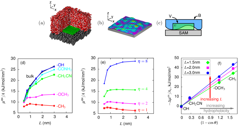
Figure 1: Size dependent hydrophobic hydration at interfaces. (a) A schematic of a cuboidal cavity (green) at the SAM-water interface. The SAM head-groups (black and white), alkane tails (grey), and water (red and white, partially cut out for clarity) are shown. (b) A typical configuration of the model membrane, color-coded by its distance from the model surface (grey). (c) Important volumes in estimating the free energy $\mu^{\text{ex}}$ of emptying the probe volume $V$ (green) using the theoretical model. The region above the membrane is the volume $B$ (blue), and the intersection of $V$ and $B$ is $v$ (dark green). (d) Lengthscale dependence of the cavity hydration free energy per unit area, $\mu^{\text{ex}}/A$, in bulk water and at interfaces, at $T=300\,$K, obtained from MD simulations. (e) $\mu^{\text{ex}}/A$, estimated using the theoretical model, near surfaces with different attraction strengths $\eta$. (f) Connecting the microscopic binding free energy of a cavity to an interface, to the macroscopic surface wettability. The $\cos\theta$ values were obtained from MD simulations of a water droplet on SAM surfaces (Shenogina et al. (2009)). Lines are predictions using Eq. (1) with size dependent $\gamma_{\rm LV}$ taken from (d).

.1 Models

Molecular simulations: We simulate the solid-water interfaces of self-assembled monolayers (SAMs) of surfactants [Fig. 1(a)] with a range of head-group chemistries, from hydrophobic (-CH₃) to hydrophilic (-OH) Godawat et al. (2009); Shenogina et al. (2009). To study the size dependence of hydration at interfaces, we selected cuboid shaped ($L\times L\times W$) cavities, with thickness $W=0.3\,$nm, and side $L$, varying from small values comparable to the size of a water molecule to as large as ten times that size. Thicker volumes will show qualitatively similar behavior, but will gradually sample the “bulk” region away from the interface.
Theoretical model: To rationalize the simulation results and obtain additional physical insights, we developed a model based on Lum-Chandler-Weeks (LCW) theory Lum et al. (1999). LCW theory incorporates the interplay between the small lengthscale gaussian density fluctuations and the physics of interface formation relevant at larger lengthscales, and captures the lengthscale dependence of hydrophobic hydration in bulk water. Near hydrophobic surfaces, it predicts the existence of a soft liquid-vapor-like interface, which has been confirmed by simulations Mittal and Hummer (2008); Godawat et al. (2009); Patel et al. (2010).

We model this liquid-vapor-like interface near a hydrophobic surface, as an elastic membrane [Fig. 1(b)], whose energetics are governed by its interfacial tension and the attractive interactions with the surface. The free energy of cavity hydration, $\mu^{\rm ex}$, is related to the probability of spontaneously emptying out a cavity shaped volume, $V$. Such emptying can be conceptualized as a two-step process in which interfacial fluctuations of the membrane can empty out a large fraction of $V$ in the first step, with the remaining volume $v$ emptied out via a density fluctuation [Fig. 1(c)]. When $v$ is small, the probability that it contains $N$ waters is well-approximated by a Gaussian Hummer et al. (1996); Crooks and Chandler (1997); Godawat et al. (2009). The cost of emptying $v$ can then be obtained from the average and the variance of number of waters in $v$, which are evaluated by assuming that the water density responds linearly to the surface-water adhesive interactions.

We tune the strength of the model surface-water attraction, $U(\mathbf{r})$, using a parameter $\eta$, where $\eta\approx 1$ corresponds to the hydrophobic $\text{-CH}_{3}$ SAM-like surface, with higher values representing increasingly hydrophilic surfaces. The representation of hydrophilic surfaces in our theoretical model lacks the specific details of hydrogen bonding interactions (e.g., between the hydrophilic -OH SAM surface and water), so comparisons between high-$\eta$ model surfaces and hydrophilic SAM surfaces in simulations are qualitative in nature. Equations that put the above model on a quantitative footing are given in the Appendix and the details of its exact implementation are included as Supplementary Information.

.2 Size-dependent hydrophobic hydration at, and binding to interfaces

Fig. 1(d) shows the excess free energy, $\mu^{\text{ex}}$, to solvate a cuboidal cavity at temperature $T=300\,$K, divided by it’s surface area ($A=2L^{2}+4LW$). $\mu^{\text{ex}}/A$ can be thought of as an effective surface tension of the cavity-water interface. In bulk water, this value shows a gradual crossover with increasing $L$, as expected Lum et al. (1999); Rajamani et al. (2005). Fig. 1(d) also shows the lengthscale dependence of $\mu^{\text{ex}}/A$ for solvating cavities in interfacial environments. Near the hydrophilic OH-terminated SAM, the behavior is similar to that in bulk water. However, with increasing hydrophobicity of the interface, the size dependence of $\mu^{\text{ex}}/A$ becomes less pronounced and is essentially absent near the -CH₃ surface, suggesting that hydration at hydrophobic surfaces is governed by interfacial physics at all lengthscales.

Fig. 1(e) shows the analogous solvation free energies predicted using the theoretical model. The essential features of solvation next to the SAM surfaces are captured well by this model. This is particularly true for the hydrophobic surfaces (with $\eta$ around $1$), where the potential $U(\mathbf{r})$ closely mimics the effect of the real SAM on the adjacent water, and the agreement between theory and simulation is nearly quantitative. For the more hydrophilic SAMs, the comparison is qualitative, because the simple form for $U(\mathbf{r})$ does not represent dipolar interactions well.

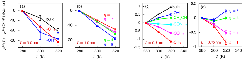
Figure 2: Temperature dependence of $\mu^{\text{ex}}$ in bulk water and at SAM-water interfaces for (a-b) large ($L=3.0\,$nm) and (c-d) small ($L=0.5\,$nm, $L=0.75\,$nm) cavities, obtained from simulations (a,c) and from the model (b,d) of Eq. (5).

Fig. 1(d) also indicates that $\mu^{\text{ex}}$ becomes favorable (smaller) with increasing surface hydrophobicity. The difference in $\mu^{\text{ex}}$ at an interface and in the bulk, $\Delta\mu^{\text{ex}}=\mu^{\text{ex}}_{\rm int}-\mu^{\text{ex}}_{\rm bulk}$, quantifies the hydration contribution to the experimentally measurable free energy of binding of solutes to interfaces. Because the solvation of large solutes is governed by the physics of interface formation, both in bulk and at the SAM surfaces, we can approximate $\Delta\mu^{\text{ex}}=A_{\rm c}(\gamma_{\rm SV}-\gamma_{\rm SL}-\gamma_{\rm LV})$, where $A_{\rm c}=L^{2}$ is the cross-sectional area, $\gamma$ is the surface tension, and subscripts SV, SL, and LV, indicate solid-vapor, solid-liquid, and liquid-vapor interfaces, respectively. Using Young’s equation, $\gamma_{\rm SV}=\gamma_{\rm SL}+\gamma_{\rm LV}\cos\theta$, we rewrite

$$\Delta\mu^{\text{ex}}=-A_{\rm c}\gamma_{\rm LV}(1-\cos\theta),$$ (1)

where $\theta$ is the water droplet contact angle on the solid surface.

Although Eq. (1) is strictly valid only for macroscopic cavities, it can be applied to sufficiently large microscopic cavitities with a lengthscale-dependent surface tension, $\tilde{\gamma}_{\rm LV}$ ($\approx\mu^{\text{ex}}_{\rm bulk}/A$). Indeed, lines in Fig. 1(f) predicted using Eq. (1) are in excellent agreement with simulation data, and indicate that the strength of binding increases with surface hydrophobicity as well as with solute size. These results establish a connection between the microscopic solute binding free energies to interfaces and the macroscopic wetting properties of those interfaces. This connection provides an approach to characterize the hydrophobicity of topographically and chemically complex interfaces, such as those of proteins Acharya et al. (2010); Giovambattista et al. (2008).

.3 Temperature dependence of hydration at interfaces

The differences between the cavity hydration at interfaces and in bulk are highlighted most clearly in the $T$-dependence of $\mu^{\text{ex}}$, which characterizes the entropic and enthalpic contributions to the free energy. For small solutes in bulk, the entropy of hydration is known to be large and negative Garde et al. (1996); Huang and Chandler (2000), which reflects the reduced configurational space available to the surrounding water molecules. In contrast, for large solutes the entropy of hydration is expected to be positive, consistent with the temperature dependence of the liquid-vapor surface tension Alejandre et al. (1995). Fig. 2(a) shows that $\mu^{\text{ex}}$ of large cuboidal cavities ($L=3\,$nm) in bulk water indeed decreases with increasing temperature, although the corresponding hydration entropy per unit surface area ($25\,$J/mol/K/nm²) is lower than that expected from the temperature derivative of surface tension of water (about $90\,$J/mol/K/nm² Alejandre et al. (1995)). We note that solvation entropies in SPC/E water obtained using NPT ensemble MD simulations are known to be smaller than experimental values by about $20$% Athawale et al. (2008). Additionally, the cavity-water surface tension and its temperature derivative for these nanoscopic cavities are expected to be smaller than the corresponding macroscopic values Patel et al. (2010).

Fig. 2(a) also shows that for large cuboidal cavities ($L=3\,$nm), $\mu^{\text{ex}}$ decreases with increasing temperature not only in bulk water and near the hydrophilic (-OH) surface, but also near the hydrophobic (-CH₃) surface, indicating a positive entropy of cavity formation. Thus, in all three systems, the thermodynamics of hydration of large cavities is governed by interfacial physics. Although the values of $\mu^{\text{ex}}(L=3\,\text{nm})$ at $300\,$K are rather large ($569\,$kJ/mol in bulk water, $565\,$kJ/mol at the -OH interface, and $167\,$kJ/mol at the -CH₃ interface), their variation with temperature shown in Fig. 2(a) is similar in bulk and at interfaces.

Fig. 2(b) shows that this same phenomenology is captured nearly quantitatively by the theoretical model. In the model, the cavity hydration free energies have large but athermal contributions from the attractions between water and the model surface. The main temperature-dependent contribution to $\mu^{\text{ex}}$ is the cost to deform the liquid-vapor-like interface near the surface to accommodate the large cavity. Since the necessary deformation is similar, regardless of the hydrophobicity of the surface, the variation of $\mu^{\text{ex}}$ with temperature is similar as well.

Fig. 2(c) shows the temperature dependence of $\mu^{\text{ex}}$ for small cavities ($L=0.5\,$nm) in bulk and at SAM-water surfaces. In bulk water, $\mu^{\text{ex}}$ increases with temperature, and yields an entropy of hydration of roughly $-25\,$J/mol/K, characteristic of small lengthscale hydrophobic hydration. This negative value is consistent with those calculated for spherical solutes of a similar volume Garde et al. (1996). With increasing hydrophobicity, the slope of the $\mu^{\text{ex}}$ vs $T$ curve decreases and becomes negative, indicating a positive entropy of cavity formation near sufficiently hydrophobic surfaces. Near the most hydrophobic surface (-CH₃), the entropy of hydration of this small cavity is $+30\,$J/mol/K.

Fig. 2(d) shows that the same phenomenon is recovered by the theoretical model, though the correspondence is clearest at a slightly larger cavity size ($L=0.75\,$nm). Near hydrophilic model surfaces, the interface is pulled close to the surface by a strong attraction, so it is costly to deform it. As a result, the cavity is emptied through bulk-like spontaneous density fluctuations that result in a negative entropy of hydration of small cavities. In contrast, near a hydrophobic surface, the interface is easy to deform, which provides an additional mechanism for creating cavities. In fact, this mechanism dominates near sufficiently hydrophobic surfaces, and since the surface tension of water decreases with increasing temperature, so does $\mu^{\text{ex}}$. Hence, even small cavities have a positive entropy of hydration near hydrophobic surfaces. The continuous spectrum of negative to positive solvation entropies observed in Figs. 2(c-d) is thus revealed to be a direct consequence of the balance between bulk-like water density fluctuations and liquid-vapor-like interfacial fluctuations.

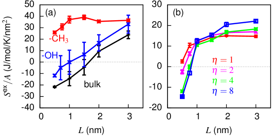
Figure 3: Lengthscale dependence of the excess solvation entropy per unit surface area for (a) cavities in bulk water and at the -CH₃ and -OH SAM-water interfaces, and (b) cavities in the model of Eq. (5) near surfaces of different attraction strengths, $\eta$.

Fig. 3(a) shows that near the hydrophobic CH₃-terminated SAM, cavity hydration entropies per unit area, $S^{\rm ex}/A$, are positive and essentially constant (about $30\,$J/mol/K/nm²) over a broad range of cavity sizes. In contrast, in bulk water, $S^{\rm ex}/A$ depends on $L$, and changes from large negative to positive values with increasing $L$. The lengthscale at which entropy crosses zero, $L_{\text{S}}$, can serve as a thermodynamic crossover length. In bulk water, $L_{\text{S}}\approx 1.8\pm 0.2\,$nm. The behavior of $S^{\rm ex}/A$ is qualitatively similar at the -OH surface, with $L_{\rm S}\approx 1.3\pm 0.4\,$nm. Although the numerical value of $L_{\text{S}}$ may depend on the shape of the cavity and on solute-water attractions for non-idealized hydrophobes, the trend in entropy should not.

Fig. 3(b) shows that our implementation of LCW ideas recovers many of the observed trends, with solvation entropy being everywhere positive for the smallest attraction strength $\eta$, and a thermodynamic crossover length of just under $1\,$nm emerging for the more hydrophilic model surfaces, similar to that in bulk water. Nevertheless, the agreement between Figs. 3(a) and (b) is somewhat qualitative, mostly as a result of the crude form of $U(\mathbf{r})$ used to model hydrophilic surfaces.

.4 Thermodynamics of binding to, and assembly at hydrophobic surfaces

In the preceding sections, we have examined the hydration behavior of single, isolated, idealized cavities near flat surfaces and in the bulk. We now consider the consequences of our observations on hydrophobically driven binding and assembly, summarized schematically in Fig. 4.

Fig. 4 indicates that while the binding of both small and large solutes (or aggregates) to hydrophobic surfaces is highly favorable, their thermodynamic signatures are different. Binding of small solutes is entropic and becomes more favorable with increasing temperature, whereas binding of large solutes is enthalpic and depends only weakly on temperature.

Fig. 4 also highlights the differences in the thermodynamics of hydrophobically driven assembly at interfaces and in bulk, inferred from our lengthscale dependence studies. In bulk, the solvation of many small, isolated hydrophobes scales as their excluded volume. Accommodating small species inside the existing hydrogen-bonding network of water imposes an entropic cost, so the solvation free energy increases with increasing temperature. When several small hydrophobes come together, water instead hydrates the aggregate by surrounding it with a liquid-vapor-like interface. The corresponding solvation free energy scales as the surface area and decreases with increasing temperature.

Thus, the driving force for assembly of $n$ small solutes (each of surface area $A_{1}$, volume $v_{1}$ and solvation free energy of $\mu_{1,\mathrm{bulk}}^{\mathrm{ex}}$) into a large aggregate (with surface area $A_{n}$ and volume $nv_{1}$) in bulk water is well-approximated by

$$\Delta\mu^{\text{ex}}_{\mathrm{bulk}}=\gamma_{\mathrm{bulk}}A_{n}-n\mu_{1,\mathrm{bulk}}^{\mathrm{ex}}=[Cn^{-1/3}-1]n\mu_{1,\mathrm{bulk}}^{\mathrm{ex}},$$ (2)

where $C\sim(\gamma_{\mathrm{bulk}}v_{1}^{2/3}/\mu_{1,\mathrm{bulk}}^{\mathrm{ex}})$ and $\gamma_{\text{bulk}}$ is a curvature-corrected effective surface tension [top curve of Fig. 1(d)]. As the surface tension decreases with increasing temperature, so does the free energy to hydrate nanometer-sized aggregates. However, the free energy to individually hydrate the small solutes increases with temperature, resulting in a larger driving force for assembly. Conversely, while the driving force for assembly, $\Delta\mu^{\text{ex}}_{\text{bulk}}$, is large and negative (favorable) at ambient conditions, it decreases in magnitude with decreasing temperature [upper portion of Fig. 4], and can even change sign at a sufficiently low temperature. When adapted to particular systems, Eq. (2) can, with remarkable accuracy, explain complex solvation phenomena like the temperature-dependent aggregation behavior of micelles Maibaum et al. (2004) and the cold denaturation of proteins Kauzmann (1959).

In the presence of a hydrophobic surface, on the other hand, we have found that interfacial physics dominates at all lengthscales [Fig. 2(a-d) and Fig. 3(a-b)]. As a result, the driving force for assembly at interfaces, $\Delta\mu^{\text{ex}}_{\mathrm{int}}$, does not scale as in Eq. (2), but is instead given by

$$\Delta\mu^{\text{ex}}_{\mathrm{int}}=\gamma_{\mathrm{int}}(A_{n}-nA_{1})\sim[n^{-1/2}-1]n\mu_{1,\mathrm{int}}^{\mathrm{ex}},$$ (3)

where $\gamma_{\mathrm{int}}$ is the effective surface tension at the interface, [the lower curves of Figs. 1(d-e)]. Since $\gamma_{\mathrm{int}}$ decreases with increasing temperature [Figs. 2(a-d)], so does the hydration contribution to the driving force for assembly at a hydrophobic surface, in contrast to that in bulk.

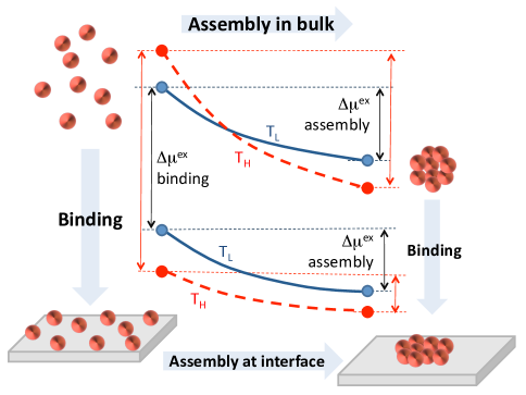
Figure 4: Schematic illustrating the thermodynamics of binding and assembly. The points represent free energies of solvating small objects individually (left) and in the assembled state (right), in bulk (top) and at a hydrophobic interface (bottom), at a lower (blue, $T_{\rm L}$) and a higher (red, $T_{\rm H}$) temperature near ambient conditions. Assembly: The driving force for assembly at hydrophobic interfaces is smaller than that in bulk. It is enthalpic and decreases with increasing temperature, unlike in bulk. Binding: The driving force for binding small objects to a hydrophobic surface increases with temperature, so it is entropic. For large objects, it is enthalpic.

The free energy barrier between disperse and assembled states is also expected to be very different in bulk and near hydrophobic surfaces. In bulk, the dispersed state has no liquid-vapor-like interface whereas the assembled state does. The transition state consists of a critical nucleus of hydrophobic particles that nucleates the liquid-vapor-like interface. The nucleation barrier can be high, and dominates the kinetics of hydrophobic collapse of idealized hydrophobic polymers ten Wolde and Chandler (2002); Miller et al. (2007); Ferguson et al. (2009) and plates Huang et al. (2005). In contrast, we expect aggregation near hydrophobic surfaces to be nearly barrierless, since an existing liquid-vapor-like interface is deformed continuously between the disperse and assembled states.

Finally, and most importantly, we find that for large aggregates, the driving force of assembly is weaker near interfaces than in bulk. In the limit of large $n$, the terms $n\mu^{\text{ex}}_{1}$ dominate both at interfaces and in bulk (Eqns. (2) and (3)), and the results in Fig. 1(d) show that $\mu^{\text{ex}}_{1,\text{int}}<\mu^{\text{ex}}_{1,\text{bulk}}$.

The nontrivial behavior of the driving forces and barriers to assembly at interfaces should be relevant in biological systems where hydrophobicity plays an important role. Experiments have shown that hydrophobic surfaces bind and facilitate the unfolding of proteins, including those that form amyloids Beverung et al. (1999); Sethuraman et al. (2004); Nikolic et al. (2011). Our results shed light on these phenomena and suggest that large hydrophobic surfaces may generically serve as catalysts for unfolding proteins Sharma et al. (2010), via solvent-mediated interactions. Indeed, simulations show that the binding of model hydrophobic polymers to hydrophobic surfaces is accompanied by a conformational rearrangement from globular to pancake-like structures Jamadagni et al. (2009). Such conformations can further assemble into secondary structures, such as $\beta$-sheets Krone et al. (2008); Sharma et al. (2010); Sethuraman et al. (2004); Nikolic et al. (2011), and we predict that the solvent contribution to this assembly at the hydrophobic surface will be governed by interfacial physics. This implies that manipulating the liquid-vapor surface tension, either by changing the temperature or by adding salts or co-solutes, will allow one to manipulate the driving force for assembly.

We further speculate that the catalysis of unfolding by hydrophobic surfaces may play a role in chaperonin function Fenton and Horwich (2003). The interior walls of chaperonins in the open conformation are hydrophobic and can bind misfolded proteins, whereupon their unfolding is catalyzed England et al. (2008); Jewett and Shea (2010). Subsequent ATP-driven conformational changes render the chaperonin walls hydrophilic England et al. (2008); Fenton and Horwich (2003). As a result, the unfolded protein is released from the wall, as the free energy for a hydrophobe to bind to a hydrophilic surface is much lower than that to bind to a hydrophobic one [Fig. 1(d)].

Our results also provide insights into the interactions between biomolecules and nonbiological hydrophobic surfaces, such as those of graphite and of certain metals, which have been shown to bind and unfold proteins Marchin and Berrie (2003); Anand et al. (2011). Such interactions are of interest in diverse applications including nano-toxicology Tian et al. (2006) and biofouling Anand et al. (2011).

Collectively, our findings highlight that assembly near hydrophobic surfaces is different from assembly in bulk and near hydrophilic surfaces. Experimental measurements of the thermodynamics of protein folding have been performed primarily in bulk water Makhatadze and Privalov (1995). Although many experiments have probed how interfaces affect protein folding, structure and function Beverung et al. (1999); Karajanagi et al. (2004), to the best of our knowledge, there are no temperature-dependent thermodynamic measurements of self-assembly at interfaces. We hope that our results will motivate such measurements.

Appendix

Simulation details: Our simulation setup and force fields are similar to that described in Refs. Shenogina et al. (2009); Godawat et al. (2009). Simulations were performed in the NVT ensemble with a periodic box ($7\,$nm$\times 7\,$nm$\times 9\,$nm) that has a buffering liquid-vapor interface at the top of the box, for reasons explained in Ref. Patel et al. (2010). It has been shown that free energies obtained in the above ensemble are indistinguishable from those obtained in the NPT ensemble at a pressure of $1\,$bar Patel et al. (2011). We have chosen the SPC/E model of water Berendsen et al. (1987) since it adequately captures experimentally known features of water, such as surface tension, compressibility, and local tetrahedral order, that play important roles in the hydrophobic effect Chandler (2005). Electrostatic interactions were calculated using the particle mesh Ewald method Essmann et al. (1995), and bonds in water were constrained using SHAKE Ryckaert et al. (1977). Solvation free energies were calculated using test particle insertions Widom (1963) for smaller cavities ($L<1\,$nm), and the indirect umbrella sampling (INDUS) method Patel et al. (2010, 2011) for larger cavities.
Theoretical Model: We model the liquid-vapor-like interface near hydrophobic surfaces as a periodic elastic membrane, $z=h(x,y)$, with an associated Hamiltonian, $H[h(x,y)]$:

$$H[h(x,y)]=\int_{x,y}\left[\frac{\gamma}{2}|\mathbf{\nabla}h(x,y)|^{2}+\int_{z=h(x,y)}^{\infty}\rho_{\ell}U(\mathbf{r})\right].$$ (4)

Here, $\gamma$ is the experimental liquid-vapor surface tension of water, $\rho_{\ell}$ is the bulk water density, and $U(\mathbf{r})$ is the interaction potential between the model surface and a water molecule at position $\mathbf{r}=(x,y,z)$. The square-gradient term in Eq. (4) accurately captures the energetics of interfacial capillary waves only for wavelengths larger than atomic dimensions (Fig. 5), so we restrict $h(x,y)$ to contain modes with wavevectors below $2\pi/9\,$Å. At any instant in time, part of $V$ can be empty due to an interfacial fluctuation. The number of waters in the remaining volume, $v$, fluctuates, and we denote by $P_{v}(N)$ the probability that $v$ contains $N$ waters. We thus estimate the free energy for emptying $V$ completely to be

$$\mu^{\text{ex}}(V)=-k_{\text{B}}T\ln\int\mathcal{D}h\,Z^{-1}e^{-\beta H[h(x,y)]}P_{v}(0),$$ (5)

where $Z=\int\mathcal{D}h\,\exp\{-\beta H[h(x,y)]\}$ is the partition function of the membrane. The volume $v$ depends on the interfacial configuration $h(x,y)$, i.e., $v=v[h(x,y)]$.

It is known that $P_{v}(N)$ is well-approximated by a Gaussian when $v$ is small Hummer et al. (1996); Crooks and Chandler (1997); Godawat et al. (2009). If water were far from liquid-vapor coexistence, then $P_{v}(N)$ would also be close to Gaussian for arbitrarily large $v$. The fact that water at ambient conditions is near liquid-vapor coexistence, and that there is a liquid-vapor-like interface near the SAM, is captured by the additional interfacial energy factor $Z^{-1}\exp\{-\beta H[h(x,y)]\}$ in Eq. (5). The net result is that the thermal average of Eq. (5) is dominated by interface configurations where $v$ is small, so that even at ambient conditions, we can approximate

$$P_{v}(N)\approx(2\pi\sigma_{v})^{-1/2}\exp\left[-(N-\langle N\rangle_{v})^{2}/2\sigma_{v}\right],$$

where $\langle N\rangle_{v}$ is the average number of waters in $v$ and $\sigma_{v}=\langle(\delta N)^{2}\rangle_{v}$ is the variance. We estimate these by noting that the solvent density responds linearly to the attractive potential, $U(\mathbf{r})$, in the volume occupied by the water, $B$, depicted in Fig. 1(c) Chandler (1993); Hummer et al. (1996); Varilly et al. (2011). Hence,

$$\langle N\rangle_{v} \approx\rho_{\ell}v-\int_{\mathbf{r}\in v}\int_{\mathbf{r}^{\prime}\in B}\,\chi(\mathbf{r},\mathbf{r}^{\prime})\beta U(\mathbf{r}^{\prime}),$$

$$\sigma_{v} \approx\int_{\mathbf{r}\in v}\int_{\mathbf{r}^{\prime}\in v}\chi(\mathbf{r},\mathbf{r}^{\prime}),\text{where}$$

$$\chi(\mathbf{r},\mathbf{r}^{\prime}) =\rho_{\ell}\delta(\mathbf{r}-\mathbf{r}^{\prime})+\rho_{\ell}^{2}[g(|\mathbf{r}-\mathbf{r}^{\prime}|)-1].$$

Here, $g(r)$ is the oxygen-oxygen radial distribution function of water Narten and Levy (1971).

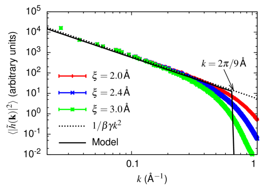
Figure 5: Power spectrum of the instantaneous liquid-vapor interface at $T=300\,$K. A liquid-vapor interface was simulated using a $24\times 24\times 3\,$nm³ slab of SPC/E water in a periodic box of size $24\times 24\times 9\,$nm³ and the instantaneous interface configuration, $h(x,y)$, and its Fourier transform, ${\tilde{h}}(\mathbf{k})$, were evaluated as in Ref. Willard and Chandler (2010). The power spectrum of our simulated instantaneous interface is good agreement with the capillary-wave theory prediction ($\langle|{\tilde{h}}(\mathbf{k})|^{2}\rangle\sim 1/\beta\gamma k^{2}$) for wavevectors smaller than $\sim 2\pi/9\,$Å. For larger wavevectors, the power spectrum is sensitive to molecular detail, i.e., the coarse-graining length $\xi$ used to define the intrinsic interface, as expected  Sedlmeier et al. (2009). Fitting the $\xi=2.0\,$Å data in the range $0.01\,\text{\AA}^{-1}<k<0.3\,\text{\AA}^{-1}$ yields $\gamma=62.0\pm 0.5\,$mJ/m², in reasonable agreement with the experimental value of $72\,$mJ/m² and some simulated values of the SPC/E surface tension (e.g., $63.6\pm 1.5\,$mJ/m² Vega and de Miguel (2007)), but not others (e.g., $52.9\,$mJ/m²  Sedlmeier et al. (2009)).

The surface–water interaction is modeled by a potential, $U(\mathbf{r})$, that closely mimics the attractive potential exterted by the $\text{-CH}_{3}$ SAM on water:

$$U(\mathbf{r})=U_{\text{wall}}(\mathbf{r})+\eta U_{\text{head}}(\mathbf{r})+U_{\text{tail}}(\mathbf{r}).$$

The first term, $U_{\text{wall}}(\mathbf{\mathbf{r}})$, is a sharply repulsive potential in the region $z<R_{0}$ that captures the hard-core exclusion of a plane of head groups at $z=0$ with hard-sphere radius $R_{0}$. The second term, $U_{\text{head}}(\mathbf{r})$, captures the head group–water interaction, modeled as a plane of OPLS/UA CH₃ Lennard-Jones (LJ) interaction sites Jorgensen et al. (1984) of area density $\mu_{\text{head}}$ at $z=0$, and is scaled by $\eta$. The final term, $U_{\text{tail}}(\mathbf{r})$, similarly captures the alkane tail–water interaction, modeled as a uniform half-space of OPLS/UA CH₂ LJ interaction sites of volume density $\rho_{\text{tail}}$ at a distance $\zeta$ below the head groups. The parameters $R_{0}$, $\zeta$, $\mu_{\text{head}}$ and $\rho_{\text{tail}}$ are dictated by the geometry of the SAM (See SI for details).

Supplementary Information

Here, we describe the details of the solvation model used in the main text.

.5 Interface description

We describe the liquid-vapor-like interface next to the model surface by a periodic height function $h({\mathbf{a}})$, with ${\mathbf{a}}=(x,y)$ and $-D/2\leq x,y<D/2$. This function is sampled discretely at a resolution $\Delta$, at points satisfying

$${\mathbf{a}}=(n_{x}\Delta,n_{y}\Delta),\qquad-\frac{D}{2\Delta}\leq n_{x},n_{y}<\frac{D}{2\Delta}.$$

This results in $N^{2}$ discrete sampling points $\{{\mathbf{a}}\}$, with $N=D/\Delta$. In the following, sums over ${\mathbf{a}}$ denote sums over these $N^{2}$ sampling points. We have used $D=60\,$Å and $\Delta=1\,$Å.

The discrete variables $\{h_{\mathbf{a}}\}$ represent the interface height at each sample point ${\mathbf{a}}$, so that

$$h_{\mathbf{a}}=h({\mathbf{a}}),\quad\text{for ${\mathbf{a}}=(n_{x}\Delta,n_{y}\Delta)$.}$$

This notation clearly distinguishes between the $N^{2}$ height variables $h_{\mathbf{a}}$ and the continuous height function $h({\mathbf{a}})$ that they represent.

The discrete Fourier transform of $\{h_{\mathbf{a}}\}$ is denoted by $\{{\tilde{h}}_{\mathbf{k}}\}$, and is defined at wavevectors ${\mathbf{k}}=(2\pi/L)(m_{x},m_{y})$, with $-N/2\leq m_{x},m_{y}<N/2$. We use the symmetric normalization convention throughout for Fourier transforms.

.6 Energetics

The essential property of the liquid-vapor-like interface is its surface tension, which results in the following capillary-wave Hamiltonian Buff et al. (1965) for a free interface,

$$H_{0}[\{h_{\mathbf{a}}\}]\approx\frac{\gamma\Delta^{2}}{2}\sum_{\mathbf{a}}|\nabla h_{\mathbf{a}}|^{2}\approx\frac{\gamma\Delta^{2}}{2}\sum_{\mathbf{k}}k^{2}|{\tilde{h}}_{\mathbf{k}}|^{2},$$

where $\nabla h_{\mathbf{a}}$ is a finite-difference approximation to $\nabla h({\mathbf{a}})$.

Using an appropriate definition of an instantaneous water-vapor interface Willard and Chandler (2010), the power spectrum of capillary waves in SPC/E water has been found to agree with the spectrum predicted by the above Hamiltonian for wavevectors smaller than about $2\pi/\ell$, but is substantially lower for higher wavevectors (Fig. 6 of main text). This result is consistent with the liquid-vapor-like interfaces being sensitive to molecular detail at high wavevectors Sedlmeier et al. (2009). At $T=300\,K$, we have found that $\ell\approx 9\,\text{\AA}.$ We thus constrain all Fourier components ${\tilde{h}}_{\mathbf{k}}$ to be zero for high ${\mathbf{k}}$, i.e.

$${\tilde{h}}_{\mathbf{k}}=0,\qquad|{\mathbf{k}}|>2\pi/\ell.$$ (6)

In our model, the liquid-vapor-like interface interacts with a model surface via a potential that depends on $\{h_{\mathbf{a}}\}$. As discussed below, it is also convenient to introduce additional umbrella potentials to aid in sampling. The Hamiltonian of the interface subject to this additional potential energy $H^{\prime}[\{h_{\mathbf{a}}\}]$ is

$$H[\{h_{\mathbf{a}}\}]=\frac{\gamma\Delta^{2}}{2}\sum_{\mathbf{k}}k^{2}|{\tilde{h}}_{\mathbf{k}}|^{2}+H^{\prime}[\{h_{\mathbf{a}}\}].$$ (7)

When expressed as a function of the Fourier components $\{{\tilde{h}}_{\mathbf{k}}\}$, we denote the Hamiltonian by ${\tilde{H}}[\{{\tilde{h}}_{\mathbf{k}}\}]$ and the external potential by ${\tilde{H}^{\prime}}[\{{\tilde{h}}_{\mathbf{k}}\}]$, so that

$${\tilde{H}}[\{{\tilde{h}}_{\mathbf{k}}\}]=\frac{\gamma\Delta^{2}}{2}\sum_{\mathbf{k}}k^{2}|{\tilde{h}}_{\mathbf{k}}|^{2}+{\tilde{H}^{\prime}}[\{{\tilde{h}}_{\mathbf{k}}\}].$$

.7 Dynamics

We calculate thermal averages of interface configurations by introducing a fictitious Langevin dynamics and replacing thermal averages by trajectory averages. We first assign a mass per unit area $\mu$ to the interface. The Lagrangian in real space is

$$L[\{h_{\mathbf{a}},{\dot{h}}_{\mathbf{a}}\}]=\frac{\mu\Delta^{2}}{2}\sum_{\mathbf{a}}{\dot{h}}_{\mathbf{a}}^{2}-H[\{h_{\mathbf{a}}\}].$$

The corresponding Lagrangian in Fourier space is

$${\tilde{L}}[\{{\tilde{h}}_{\mathbf{k}},{\dot{\tilde{h}}}_{\mathbf{k}}\}]=\frac{\mu\Delta^{2}}{2}\sum_{\mathbf{k}}|{\dot{\tilde{h}}}_{\mathbf{k}}|^{2}-{\tilde{H}}[\{{\tilde{h}}_{\mathbf{k}}\}].$$

Since all $h_{\mathbf{a}}$ are real, the amplitudes of modes ${\mathbf{k}}$ and $-{\mathbf{k}}$ are related, ${\tilde{h}}_{\mathbf{k}}={\tilde{h}}^{*}_{-{\mathbf{k}}}.$ Taking this constraint and Equation (6) into account, the Euler-Lagrange equations yield equations of motion in Fourier space. To thermostat each mode, we add Langevin damping and noise terms. The final equation of motion has the form

$$\mu\Delta^{2}{\ddot{\tilde{h}}}_{\mathbf{k}}=-\gamma\Delta^{2}|{\mathbf{k}}|^{2}{\tilde{h}}_{\mathbf{k}}-\frac{\partial{\tilde{H}^{\prime}}[\{{\tilde{h}}_{\mathbf{k}}\}]}{\partial{\tilde{h}}_{\mathbf{k}}}-\eta{\dot{\tilde{h}}}_{\mathbf{k}}+{\tilde{\xi}}_{\mathbf{k}}(t),\qquad(|{\mathbf{k}}|<2\pi/\ell),$$ (8)

The Langevin damping constant $\eta$ is chosen to decorrelate momenta over a timescale $\tau$, so $\eta=\mu\Delta^{2}/\tau.$ The zero-mean Gaussian noise terms $\{{\tilde{\xi}}_{\mathbf{k}}(t)\}$ have variance such that

$$\langle{\tilde{\xi}}^{*}_{\mathbf{k}}(t){\tilde{\xi}}_{\mathbf{k}}(t^{\prime})\rangle=2\eta k_{\text{B}}T\delta(t-t^{\prime}).$$

As with ${\tilde{h}}_{\mathbf{k}}$, ${\tilde{\xi}}_{\mathbf{k}}$ satisfy the related constraint ${\tilde{\xi}}_{\mathbf{k}}={\tilde{\xi}}^{*}_{-{\mathbf{k}}}$. Hence, for ${\mathbf{k}}={\mathbf{0}}$, the noise is purely real and its variance is twice that of the real and imaginary components of all other modes.

We propagate these equations of motion using the Velocity Verlet algorithm. At each force evaluation, we use a Fast Fourier Transform (FFT) to calculate $\{h_{\mathbf{a}}\}$ from $\{{\tilde{h}}_{\mathbf{k}}\}$. We then calculate $\partial H^{\prime}[\{h_{\mathbf{a}}\}]/\partial h_{\mathbf{a}}$ in real space and perform an inverse FFT to obtain the force $\partial{\tilde{H}^{\prime}}[\{{\tilde{h}}_{\mathbf{k}}\}]/\partial{\tilde{h}}_{\mathbf{k}}$ on mode ${\tilde{h}}_{\mathbf{k}}$ due to $H^{\prime}[\{h_{\mathbf{a}}\}]$. We then add the forces due to surface tension, Langevin damping and thermal noise, as in Eq. (8).

For the Velocity Verlet algorithm to be stable, we choose a timestep equal to $1/20^{\text{th}}$ of the typical timescale of the highest-frequency mode of the free interface, $\Delta t=\frac{1}{20}\sqrt{\mu\ell^{2}/\gamma}.$ To equilibrate the system quickly but still permit natural oscillations, we choose the Langevin damping timescale so that $\tau=100\Delta t.$ Finally, we choose a value of $\mu$ close to the mass of a single water layer, $\mu=100\,\text{amu}/\text{nm}^{2}.$

This interface dynamics is entirely fictitious. However, it correctly samples configurations of the interface Boltzmann-weighted by the Hamiltonian $H[\{h_{\mathbf{a}}\}]$. This is true regardless of the exact values of $\mu$, $\Delta t$ and $\tau$, so our choices have no effect on the results in the main text. We have simply chosen reasonable values that do not lead to large discretization errors when solving the system’s equations of motion.

.8 Surface-interface interactions

The liquid-vapor-like interface interacts with the model surface via a potential $H^{\prime}_{\text{surf}}[\{h_{\mathbf{a}}\}]$. In the atomistic simulations, the SAM sets up an interaction potential $U({\mathbf{r}})$ felt by the atoms in the water molecules. Below, we use the notation ${\mathbf{r}}$ and $(x,y,z)$ interchangeably. To model this interaction potential, we smear out the atomistic detail of the SAM and replace it with three elements:

• A uniform area density $\mu_{\text{head}}$ of Lennard-Jones sites (with length and energy scales $\sigma_{\text{head}}$ and $\epsilon_{\text{head}}$) in the $z=0$ plane to represent the SAM head groups.

• A uniform volume density $\rho_{\text{tail}}$ of Lennard-Jones sites (with length and energy scales $\sigma_{\text{tail}}$ and $\epsilon_{\text{tail}}$) in the half-space $z<-\zeta$ to represent the SAM tail groups.

• Coarse-graining the head-group atoms into a uniform area density results in a softer repulsive potential allowing the interface to penetrate far deeper into the model surface than would be possible in the actual SAM. To rectify this, we apply a strongly repulsive linear potential in the half-space $z<R_{0}$, where $R_{0}$ is the radius of the head group’s hard core. The repulsive potential is chosen to be $1\,k_{\text{B}}T$ when $1\,$nm² of interface penetrates the region $z<R_{0}$ by a “skin depth” $\delta$.

The head groups are thus modeled by the following potential acting on a water molecule at position ${\mathbf{r}}$:

$$U_{\text{head}}(x,y,z\geq R_{0})=\mu_{\text{head}}\int_{-\infty}^{\infty}\text{d}x^{\prime}\,\int_{-\infty}^{\infty}\text{d}y^{\prime}\,u_{\text{LJ}}\left(|{\mathbf{r}}-{\mathbf{r}}^{\prime}|;\epsilon_{\text{head}},\sigma_{\text{head}}\right)\big{|}_{z^{\prime}=0},$$

where $u_{\text{LJ}}(r;\epsilon,\sigma)=4\epsilon[(\sigma/r)^{12}-(\sigma/r)^{6}]$ is the Lennard-Jones pair potential. Similarly, the effect of the tail groups is captured by

$$U_{\text{tail}}(x,y,z\geq R_{0})=\rho_{\text{tail}}\int_{-\infty}^{\infty}\text{d}x^{\prime}\,\int_{-\infty}^{\infty}\text{d}y^{\prime}\,\int_{-\infty}^{-\zeta}\text{d}z^{\prime}\,u_{\text{LJ}}\left(|{\mathbf{r}}-{\mathbf{r}}^{\prime}|;\epsilon_{\text{tail}},\sigma_{\text{tail}}\right).$$

Finally, the repulsive wall is modeled by the potential

$$U_{\text{wall}}(x,y,z<R_{0})=2\rho_{\ell}^{-1}\cdot(1\,k_{\text{B}}T/1\,\text{nm}^{2})(R_{0}-z)/\delta,$$

where $\rho_{\ell}=0.03333\,\text{\AA}^{-3}$ is the number density of liquid water.

These smeared interaction potentials depend only on $z$, not on $x$ or $y$. As described in the main text, we also scale the head-group interaction by a parameter $\eta$. Putting everything together, we obtain an explicit expression for the surface-interface interaction potential,

$$H^{\prime}_{\text{surf}}[\{h_{\mathbf{a}}\}]=\rho_{\ell}\Delta^{2}\sum_{\mathbf{a}}h^{\prime}_{\text{surf}}(h_{\mathbf{a}}),$$

where

$$h^{\prime}_{\text{surf}}(h_{\mathbf{a}}) =\int_{h_{\mathbf{a}}}^{\infty}\text{d}z\,\eta U_{\text{head}}(z)+U_{\text{tail}}(z)+U_{\text{wall}}(z),$$

$$=\begin{cases}\eta\pi\epsilon_{\text{head}}\mu_{\text{head}}\sigma_{\text{head}}^{3}\left[\frac{4}{45}(\sigma_{\text{head}}/z)^{9}-\frac{2}{3}(\sigma_{\text{head}}/z)^{3}\right]&\\ \quad+\pi\epsilon_{\text{tail}}\rho_{\text{tail}}\sigma_{\text{tail}}^{4}\left[\frac{1}{90}(\sigma_{\text{head}}/[z+\zeta])^{8}-\frac{1}{3}(\sigma_{\text{head}}/[z+\zeta])^{2}\right],&z\geq R_{0},\\ h^{\prime}_{\text{surf}}(R_{0})+\rho_{\ell}^{-1}\cdot(1\,k_{\text{B}}T/1\,\text{nm}^{2})([R_{0}-z]/\delta)^{2},&z<R_{0}.\end{cases}$$

To model the -CH₃ SAM in this paper, we chose the following values for the parameters

• The head groups are modeled as OPLS united-atom CH₃ groups interacting with SPC/E water, so $\sigma_{\text{head}}=3.5355\,$Å and $\epsilon_{\text{tail}}=0.68976\,$kJ/mol.

• The tail groups are modeled as OPLS united-atom CH₂ groups (sp³-hybridized) interacting with SPC/E water, so $\sigma_{\text{tail}}=3.5355\,$Å and $\epsilon_{\text{tail}}=0.5664\,$kJ/mol.

• The tail region is inset from the plane of the head groups by a distance equal to a CH₂-CH₃ bond length ($1.50\,$Å), minus the van der Waals radius of a CH₂ group ($1.9525\,$Å), so $\zeta=-0.4525\,$Å.

• The head group density is known from the atomistic SAM geometry to be $\mu_{\text{head}}=0.0462\,$Å^-2. The mass density of the SAM tails was estimated to be $935\,$kg/m³ Godawat et al. (2009), resulting in a CH₂ group number density of $\rho_{\text{tail}}=0.0402\,$Å^-3.

• The equivalent hard sphere radius $R_{0}$ of a -CH₃ group at room temperature was estimated to be $3.37\,$Å Patel et al. (2010). It has a small temperature dependence, which we neglect.

• The wall skin depth $\delta$ was set to $0.1\,$Å, which is small enough so that the repulsive potential is essentially a hard wall at $z=R_{0}$, but large enough that we can propagate the interfacial dynamics with a reasonable timestep.

.9 Umbrella sampling

Calculating $\mu^{\text{ex}}(V)$ from Equation (2) of the main text as a thermal average $\langle P_{v}(0)\rangle$ over Boltzmann-weighted configurations of $h({\mathbf{a}})$ is impractical for large $V$. The configurations that dominate this average simply have a vanishingly small Boltzmann weight. To solve this problem, and in analogy to what we do in atomistic simulations, we perform umbrella sampling on the size of the sub-volume $v$ of the probe cavity $V$ that is above the interface.

We begin by defining the volume $V$ corresponding to a probe cavity of dimensions $L\times L\times W$ as the set of points satisfying $|x|,|y|\leq L/2$ and $R_{0}\leq z\leq R_{0}+W$. We then define $v[\{h_{\mathbf{a}}\}]$ as the size of the sub-volume of $V$ that is above the interface. Using umbrella sampling and the multistate Bennet acceptance ratio method (MBAR) Shirts and Chodera (2008), we calculate the probability distribution for $v$, $P(v)$, down to $v=0$. To do this, we use quadratic umbrellas defined by a center $\bar{v}$ and width $(\delta v)^{2}$, which result in the addition to the Hamiltonian of

$$H^{\prime}_{\text{umb}}[\{h_{\mathbf{a}}\}]=k_{\text{B}}T\,\frac{(v[\{h_{\mathbf{a}}\}]-\bar{v})^{2}}{2(\delta v)^{2}}.$$

During each umbrella run, we also record the configurations $\{h_{\mathbf{a}}\}$ which yield each observed value of $v$. We then approximate the right-hand side of Equation (2) in the main text by summing over these configurations with appropriate weights, and obtain

$$\mu^{\text{ex}}(V)\approx-k_{\text{B}}T\ln\frac{\sum_{\{h_{\mathbf{a}}\}}P_{v}(0)P(v[\{h_{\mathbf{a}}\}])}{\sum_{\{h_{\mathbf{a}}\}}P(v[\{h_{\mathbf{a}}\}])},$$

where, as in the main text, the term $P_{v}(0)$ depends on the interface configuration $\{h_{\mathbf{a}}\}$, and the sum $\{h_{\mathbf{a}}\}$ is over all interface configurations in all the different umbrellas. To evaluate $P_{v}(0)$, we implement discrete versions of the integrals defining $\langle N\rangle_{v}$ and $\sigma_{v}$ as was done in Ref. Varilly et al. (2011).

References

- Tanford (1973) C. Tanford, The Hydrophobic Effect - Formation of Micelles and Biological Membranes (Wiley Interscience, New York, 1973).
- Kauzmann (1959) W. Kauzmann, Adv. Prot. Chem., 14, 1 (1959).
- Stillinger (1973) F. H. Stillinger, J. Solution Chem., 2, 141 (1973).
- Lum et al. (1999) K. Lum, D. Chandler, and J. D. Weeks, J. Phys. Chem. B, 103, 4570 (1999).
- Chandler (2005) D. Chandler, Nature, 437, 640 (2005).
- Mittal and Hummer (2008) J. Mittal and G. Hummer, P. Natl. Acad. Sci. U.S.A., 105, 20130 (2008).
- Godawat et al. (2009) R. Godawat, S. N. Jamadagni, and S. Garde, P. Natl. Acad. Sci. U.S.A., 106, 15119 (2009).
- Patel et al. (2010) A. J. Patel, P. Varilly, and D. Chandler, J. Phys. Chem. B, 114, 1632 (2010).
- Shenogina et al. (2009) N. Shenogina, R. Godawat, P. Keblinski, and S. Garde, Phys. Rev. Lett., 102, 156101 (2009).
- Hummer et al. (1996) G. Hummer, S. Garde, A. E. Garcia, A. Pohorille, and L. R. Pratt, P. Natl. Acad. Sci. U.S.A., 93, 8951 (1996).
- Crooks and Chandler (1997) G. E. Crooks and D. Chandler, Phys. Rev. E, 56, 4217 (1997).
- Rajamani et al. (2005) S. Rajamani, T. M. Truskett, and S. Garde, P. Natl. Acad. Sci. U.S.A., 102, 9475 (2005).
- Acharya et al. (2010) H. Acharya, S. Vembanur, S. N. Jamadagni, and S. Garde, Faraday Discuss., 146, 353 (2010).
- Giovambattista et al. (2008) N. Giovambattista, C. F. Lopez, P. J. Rossky, and P. G. Debenedetti, P. Natl. Acad. Sci. U.S.A., 105, 2274 (2008).
- Garde et al. (1996) S. Garde, G. Hummer, A. E. Garcia, M. E. Paulaitis, and L. R. Pratt, Phys. Rev. Lett., 77, 4966 (1996).
- Huang and Chandler (2000) D. M. Huang and D. Chandler, P. Natl. Acad. Sci. U.S.A., 97 (2000).
- Alejandre et al. (1995) J. Alejandre, D. J. Tildesley, and G. A. Chapela, J. Chem. Phys., 102, 4574 (1995).
- Athawale et al. (2008) M. V. Athawale, S. Sarupria, and S. Garde, J. Phys. Chem. B, 112, 5661 (2008).
- Maibaum et al. (2004) L. Maibaum, A. R. Dinner, and D. Chandler, J. Phys. Chem. B, 108, 6778 (2004).
- ten Wolde and Chandler (2002) P. R. ten Wolde and D. Chandler, P. Natl. Acad. Sci. U.S.A., 99, 6539 (2002).
- Miller et al. (2007) T. Miller, E. Vanden-Eijnden, and D. Chandler, P. Natl. Acad. Sci. U.S.A., 104, 14559 (2007).
- Ferguson et al. (2009) A. L. Ferguson, P. G. Debenedetti, and A. Z. Panagiotopoulos, J. Phys. Chem. B, 113, 6405 (2009).
- Huang et al. (2005) X. Huang, R. Zhou, and B. J. Berne, J. Phys. Chem. B, 109, 3546 (2005).
- Beverung et al. (1999) C. J. Beverung, C. J. Radke, and H. W. Blanch, Biophys. Chem., 81, 59 (1999).
- Sethuraman et al. (2004) A. Sethuraman, G. Vedantham, T. Imoto, T. Przybycien, and G. Belfort, Proteins, 56, 669 (2004).
- Nikolic et al. (2011) A. Nikolic, S. Baud, S. Rauscher, and R. Pomes, Proteins, 79, 1 (2011).
- Sharma et al. (2010) S. Sharma, B. J. Berne, and S. K. Kumar, Biophys. J., 99, 1157 (2010).
- Jamadagni et al. (2009) S. N. Jamadagni, R. Godawat, J. S. Dordick, and S. Garde, J. Phys. Chem. B, 113, 4093 (2009).
- Krone et al. (2008) M. G. Krone, L. Hua, P. Soto, R. Zhou, B. J. Berne, and J.-E. Shea, J. Am. Chem. Soc., 130, 11066 (2008).
- Fenton and Horwich (2003) W. Fenton and A. Horwich, Q. Rev. Biophys., 36, 229 (2003).
- England et al. (2008) J. England, D. Lucent, and V. Pande, Curr. Opin. Struc. Biol., 18, 163 (2008).
- Jewett and Shea (2010) A. Jewett and J.-E. Shea, Cell. Mol. Life Sci., 67, 255 (2010).
- Marchin and Berrie (2003) K. L. Marchin and C. L. Berrie, Langmuir, 19, 9883 (2003).
- Anand et al. (2011) G. Anand, F. Zhang, R. J. Linhardt, and G. Belfort, Langmuir, 27, 1830 (2011).
- Tian et al. (2006) F. Tian, D. Cui, H. Schwarz, G. G. Estrada, and H. Kobayashi, Toxicology in Vitro, 20, 1202 (2006).
- Makhatadze and Privalov (1995) G. Makhatadze and P. Privalov, Adv. Prot. Chem., 47, 307 (1995).
- Karajanagi et al. (2004) S. S. Karajanagi, A. A. Vertegel, R. S. Kane, and J. S. Dordick, Langmuir, 20, 11594 (2004).
- Patel et al. (2011) A. J. Patel, P. Varilly, D. Chandler, and S. Garde, J. Stat. Phys., submitted (2011).
- Berendsen et al. (1987) H. J. C. Berendsen, J. R. Grigera, and T. P. Straatsma, J. Phys. Chem., 91, 6269 (1987).
- Essmann et al. (1995) U. Essmann, L. Perera, M. L. Berkowitz, T. Darden, H. Lee, and L. G. Pedersen, J. Chem. Phys., 103, 8577 (1995).
- Ryckaert et al. (1977) J.-P. Ryckaert, G. Ciccotti, and H. J. C. Berendsen, J. Comp. Phys., 23, 327 (1977).
- Widom (1963) B. Widom, J. Chem. Phys., 39, 2808 (1963).
- Chandler (1993) D. Chandler, Phys. Rev. E, 48, 2898 (1993).
- Varilly et al. (2011) P. Varilly, A. J. Patel, and D. Chandler, J. Chem. Phys., 134, 074109 (2011).
- Narten and Levy (1971) A. H. Narten and H. A. Levy, J. Chem. Phys., 55, 2263 (1971).
- Willard and Chandler (2010) A. P. Willard and D. Chandler, J. Phys. Chem. B, 114, 1954 (2010).
- Sedlmeier et al. (2009) F. Sedlmeier, D. Horinek, and R. R. Netz, Phys. Rev. Lett., 103, 136102 (2009).
- Vega and de Miguel (2007) C. Vega and E. de Miguel, J. Chem. Phys., 126, 154707 (2007).
- Jorgensen et al. (1984) W. L. Jorgensen, J. D. Madura, and C. J. Swenson, J. Am. Chem. Soc., 106, 6638 (1984).
- Buff et al. (1965) F. Buff, R. Lovett, and F. H. Stillinger, Phys. Rev. Lett., 15, 621 (1965).
- Note (1) The constraint on the magnitude of ensures that no Nyquist modes, i.e., modes with or equal to , are ever excited. If they were included, these modes would also be purely real, and the variance of the real component of their noise terms would likewise be twice that of the real component of the interior modes.
- Shirts and Chodera (2008) M. R. Shirts and J. D. Chodera, J. Chem. Phys., 129, 124105 (2008).