Use of the attractive hard-core Yukawa interaction for the derivation of the phase diagram of liquid water.

Abstract

The phase diagram of the attractive hard-core Yukawa fluid derived previously [M. Robles and M. López de Haro, J. Phys. Chem. C 111, 15957 (2007)] is used to obtain the liquid-vapor coexistence curve of real water. To this end, the value of the inverse range parameter of the intermolecular potential in the Yukawa fluid is fixed so that the ratio of the density at the critical point to the liquid density at the triple point in this model coincides with the same ratio in water. Subsequently, a (relatively simple) nonlinear rescaling of the temperature is performed which allows one to obtain the full liquid vapor coexistence curve of real water in the temperature-density plane with good accuracy, except close to the triple point. Such rescaling may be physically interpreted in terms of an effective temperature-dependent attractive hard-core Yukawa interaction potential which in turn introduces an extra temperature dependence in the equation of state. With the addition of a multiplicative factor to obtain from the model the critical pressure of real water, the corrected equation of state yields reasonably accurate isotherms in the liquid phase region except in the vicinity of the critical isotherm and in the vicinity of the triple point isotherm. The liquid-vapor coexistence curves in the pressure-temperature and pressure-density planes are also computed and a possible way to improve the quantitative agreement with the real data is pointed out.

1 Introduction

Due to its ubiquitous presence and importance both in our everyday life and in nature, water has been the subject of numerous experimental and theoretical studies[1]. Yet, despite all of this work, the full understanding of its properties is still far from complete and new efforts are called for.

Out of the many interesting and puzzling aspects of the properties of water, a particular challenging and still open problem is the determination of the full phase diagram of the system. In fact, a stringent test of many theoretical models is often their predicted phase diagram. In this paper, we will consider an aspect of this problem, namely the possibility of using a relatively simple model to obtain a sensible description of the liquid phase and the saturation curve of liquid water. Concerning the fluid region, the International Association for the Properties of Water and Steam from time to time issues documents on their recommended formulation for the thermodynamic properties of ordinary water substance for general and scientific use, the most recent one[2] dated in September 2009 and related to the so called IAPWS Formulation 1995[3]. This formulation consists of a fundamental equation for the Helmholtz free energy of water which is obtained from a sophisticated fitting procedure of a wealth of experimental results. It is claimed to be valid in the fluid region up to temperatures of 1273 K and pressures up to 1000 MPa and to represent very well the most accurate experimental data in the single phase region and on the vapor-liquid phase boundary. On the computational side, a rather successful model is the TIP4P model[4] or its modified version the TIP4P/2005 model[5]. This is a simple rigid nonpolarizable model with a Lennard-Jones site on the oxygen and partial positive charges on the hydrogen atoms. Further, the negative charge is placed along the bisector of the H-O-H bond and the parameters in the potential are adjusted to match the experimental density and the enthalpy of vaporization of liquid water. The TIP4P/2005 model in particular provides an excellent description of the coexisting densities along the orthobaric curve but it fails to yield the correct critical pressure. As a final piece of information required for the purposes of this work, mention should be made here of the analytic equation of state of liquid water introduced by Jeffery and Austin[6]. Such an equation of state is based on the principle of corresponding states of Ihm, Song and Mason[7] and on the free energy of strong tetrahedral hydrogen bonds proposed by Poole et al[8]. It is accurate and probably useful for engineering calculations but contains many adjustable parameters which is clearly an undesirable feature.

Recently[9], using thermodynamic perturbation theory and a hard-sphere (HS) fluid as the reference system, we have derived an approximate equation of state for the attractive hard-core Yukawa (HCY) fluid and computed the corresponding phase diagram in the three different thermodynamic planes. This model fluid, which has received a lot of attention in different contexts,[10] is interesting because in certain well defined limits its interaction potential has proved to yield thermodynamically equivalent results to those of the Lennard-Jones potential, the Coulombic interaction, the HS potential, or the adhesive HS potential. The main asset of our derivation lies in the fact that the results are analytical and have a rather simple form. What we want to do here is to take advantage of the above mentioned properties and use these results to obtain a reasonable description of liquid water (including the vapor-liquid coexistence curve) with a simple model. In this way we want to provide, albeit with limitations, a positive answer to the question raised in the provocative title (“Can simple models describe the phase diagram of water?”) of a recent paper by Vega et al[11].

The paper is organized as follows. In order to make it self-contained, in the next section we provide the equation of state of the attractive HCY fluid. This is followed in Sect. 3 with the description of the procedure to map the results of the attractive HCY fluid to those of real water in the fluid phase. Section 4 is devoted to the mapping of the liquid-vapor coexistence curve in the pressure-density and pressure-temperature planes. The paper is closed in Sect. 5 with further discussion and some concluding remarks.

2 Approximate equation of state for the attractive HCY fluid.

The attractive HCY fluid is a system whose molecules interact via the pair potential

$$\phi_{{HCY}}\left(r\right)=\left\{\begin{array}[]{cc}\infty,&r\leq\sigma\\ -\epsilon\frac{\sigma}{r}\exp[-z(r-\sigma)/\sigma],&r>\sigma\end{array}\right.,$$ (1)

where $\sigma$ is the hard-core diameter, $\epsilon$ is the depth of the potential well at $r=\sigma$, and $z$ is the (dimensionless) inverse range parameter.

The potential $\phi_{{HCY}}\left(r\right)$ may be split in a form convenient for the use of the liquid state perturbation theory as $\phi_{{HCY}}\left(r\right)=\phi_{0}\left(r\right)+\phi_{1}\left(r\right)$, where the reference potential $\phi_{0}$ will be a HS pair potential (where the “effective” diameter $d$ of the HS reference system will simply coincide with the hard-core diameter, $\sigma$), and the perturbed part $\phi_{1}$ is given by

$$\phi_{1}\left(r\right)=\left\{\begin{array}[]{cc}0,&r\leq\sigma\\ -\epsilon\frac{\sigma}{r}\exp[-z(r-\sigma)/\sigma],&r>\sigma\end{array}\right.$$ (2)

Next we consider the usual perturbative expansion [12] for the (excess) Helmholtz free energy $A^{{ex}}_{{HCY}}$ of this fluid. To first order in $\beta\equiv 1/k_{B}T$, with $T$ the absolute temperature and $k_{B}$ the Boltzmann constant, its approximate expression reads (for details see Ref. [9])

$$\frac{A^{{ex}}_{{HCY}}}{Nk_{B}T}=\frac{A^{{ex}}_{{HS}}}{Nk_{B}T}-12\eta\beta\epsilon e^{z}G(z),$$ (3)

where

$$\frac{A^{{ex}}_{{HS}}}{Nk_{B}T}=\int_{0}^{\eta}\frac{Z_{{HS}}(\eta^{\prime})-1}{\eta^{\prime}}d\eta^{\prime}$$ (4)

is the (excess) free energy of the HS fluid, $Z_{{HS}}(\eta)\equiv 1+4\eta g_{{HS}}(\sigma^{+})$ is the compressibility factor of the HS fluid, $\eta=\frac{\pi}{6}\rho\sigma^{3}$ is the packing fraction ($\rho$ being the density and $N$ the number of particles), $g_{{HS}}(\sigma^{+})$ is the contact value of the HS radial distribution function and $G(z)\equiv G(t=z)$ with $G(t)={{\mathcal{L}}}[rg_{{HS}}(r)]$, ${\mathcal{L}}$ denoting the Laplace transform operator. Here $g_{{HS}}(r)$ stands for the radial distribution function of the HS fluid.

Within the rational function approximation method[13], $G(t)$ turns out to be be given by

$${G(t)=\frac{t}{12\eta}\frac{1}{1-e^{t}\Phi(t)}}$$ (5)

where $\Phi(t)$ is a rational function of the form

$${\Phi(t)=\frac{1+S_{1}t+S_{2}t^{2}+S_{3}t^{3}+S_{4}t^{4}}{1+L_{1}t+L_{2}t^{2}}}$$ (6)

and the coefficients $S_{i}$ and $L_{i}$ are the following functions of the packing fraction $\eta$

$${\ L_{1}} = {\frac{1}{2}\frac{\eta+12\eta L_{2}+2-24\eta S_{4}}{2\eta+1},}$$ (7)

$${L_{2}} = {-3\left(Z_{{HS}}-1\right)S_{4},}$$ (8)

$${\ S_{1}} = {\frac{3}{2}\eta\frac{-1+4L_{2}-8S_{4}}{2\eta+1},}$$ (9)

$${S_{2}} = -{\frac{1}{2}\frac{-\eta+8\eta L_{2}+1-2L_{2}-24\eta S_{4}}{2\eta+1},}$$ (10)

$${S_{3}} = {\frac{1}{12}\frac{2\eta-\eta^{2}+12\eta L_{2}(\eta-1)-1-72\eta^{2}S_{4}}{\left(2\eta+1\right)\eta},}$$ (11)

$${S_{4}} = {\frac{1-\eta}{36\eta\left(Z_{{HS}}-1/3\right)}\left[1-\left[1+\frac{Z_{{HS}}-1/3}{Z_{{HS}}-Z_{{PY}}}\left(\frac{\chi_{{HS}}}{\chi_{{PY}}}-1\right)\right]^{1/2}\right],}$$ (12)

with, $Z_{{PY}}=\frac{1+2\eta+3\eta^{2}}{\left(1-\eta\right)^{2}}$, $\chi_{{PY}}=\frac{\left(1-\eta\right)^{4}}{\left(1+2\eta\right)^{2}}$ and $\chi_{{HS}}\equiv\left(\frac{d}{d\eta}[\eta Z_{{HS}}]\right)^{-1}$. Note then that the only input required to completely determine $A^{{ex}}_{{HCY}}$ is an expression for $Z_{{HS}}$. Here we will consider the compressibility factor that follows from the popular Carnahan-Starling equation of state given by [14]

$$Z_{{HS}}(\eta)=\frac{1+\eta+\eta^{2}-\eta^{3}}{\left(1-\eta\right)^{3}},$$ (13)

which is known to be rather accurate in the stable fluid region. This in turn implies that in this case

$$\chi_{{HS}}(\eta)=\frac{\left(1-\eta\right)^{4}}{1+4\eta+4\eta^{2}-4\eta^{3}+\eta^{4}}.$$ (14)

From Eqs. (3) – (13) one may easily derive the explicit form of the equation of state of the attractive HCY fluid in terms of the dimensionless variables $\bar{P}=P\sigma^{3}/\epsilon$ ($P$ being the pressure), $\bar{\rho}=\rho\sigma^{3}$ and $\bar{T}=k_{B}T/\epsilon$, namely

$$\bar{P}=\bar{\rho}\bar{T}Z_{{HS}}\left(\frac{\pi}{6}\bar{\rho}\right)-2\pi{\bar{\rho}}^{2}e^{z}\frac{\partial}{\partial\bar{\rho}}\left[\bar{\rho}G(z)\right],$$ (15)

where it is understood that the packing fraction $\eta$ appearing in all the expressions related to $G(z)$ must be replaced by $\frac{\pi}{6}\bar{\rho}$.

The (approximate) phase diagram of the attractive HCY fluid in the three thermodynamic planes ($\bar{T}$-$\bar{\rho}$, $\bar{P}$-$\bar{T}$ and $\bar{P}$-$\bar{\rho}$) was obtained using Eq. (15) and compared to simulation data in Ref. [9]. Such a comparison indicated that the approximate equation of state was a reasonable compromise between accuracy and simplicity. With this in mind, in the next section we will try to use the same equation of state to obtain the phase diagram of water in the stable fluid region.

3 Scaling for the thermodynamics of water

The length and energy units for the attractive HCY fluid are defined arbitrarily by the parameters $\sigma$ and $\epsilon$ in the interaction potential. The parameter $z$ plays the role of an adjustable free parameter needed in any application of the model. To map the attractive HCY fluid to the real thermodynamic properties of water, we have taken the following steps:

• To fix the value of $z$ in the way specified below.

• To find a non-linear rescaling of the temperature to fit the saturation branch of the coexistence curve.

• To compare the rescaled attractive HCY fluid isotherms with those of real water.

• To adjust the value of the critical pressure of the attractive HCY fluid to match the one of real water.

3.1 The choice of the inverse range parameter

In our previous work,[9] we discussed how to obtain, for a given $z$, the liquid-vapor coexistence curve for the attractive HCY fluid through the usual Maxwell construction in the $\bar{T}$-$\bar{\rho}$ plane. Now we want to determine the value of $z$ such that the coexistence curve derived for the attractive HCY fluid may be used for water. For this purpose it is convenient to introduce the reduced quantities $T^{*}=T/T_{c}$ and $\rho^{*}=\rho/\rho_{t}$, where $T_{c}$ and $\rho_{t}$ are the critical temperature and liquid density at the triple point, respectively. In what follows we will add to the subscripts the labels $w$ and $Y$ to indicate real water and attractive HCY fluid, respectively. For water, we take $T_{wc}=647.096$ K and $\rho_{wt}=999.793$ kg/m³.[17] It should be pointed out that for our approximate equation of state for the attractive HCY fluid, Eq. (15), the density at the triple point is independent of $z$ and is given by $\bar{\rho}_{Yt}=0.9375$. [15] On the other hand, the critical density and temperature for the attractive HCY fluid only depend on $z$. We next fix $z$ by requiring that the ratio $\rho_{Yc}/\rho_{Yt}$ of the attractive HCY fluid coincides with the reduced critical density of water, $\rho_{wc}/\rho_{wt}=0.32207$. In this way, the resulting value of the inverse range parameter is $z=1.7118$ which yields $\bar{T}_{Yc}=1.35997$ and $\bar{\rho}_{Yc}=0.3019$. Since $\bar{T}_{Yc}=k_{B}T_{c}/\epsilon_{c}$ (where we have added a subscript c to $\epsilon$ for reasons that will become clear later) and $\bar{\rho}_{Yt}=\rho_{wt}\sigma^{3}$, we get $\epsilon_{c}\simeq 6.57\times 10^{-21}$ J and $\sigma\simeq 3.0401\times 10^{-10}$ m. Therefore we now have all the quantities required for the comparison of the two coexistence curves. In figure 1 we show the liquid-vapor coexistence curves in the $T^{*}$-$\rho^{*}$ plane for both real water and the corresponding attractive HCY fluid with the above value of $z$.

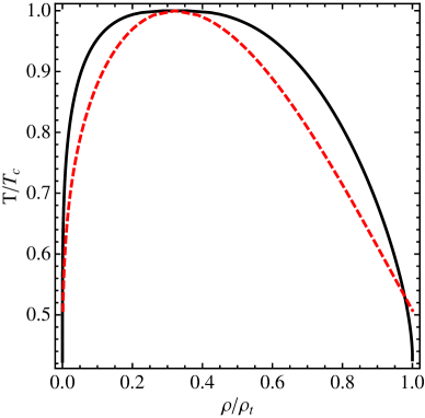
Figure 1: Coexistence liquid-vapor curves for real water (continuous line) and the fitted attractive HCY fluid with $z=1.7118$ (red dashed line).

Note that the shape of the two curves is similar. Nevertheless, one still has to manipulate the data if a better quantitative agreement is desired. Undoubtedly, the best way would be to follow a crossover treatment[18] incorporating the scaling laws valid for the critical region, as has been done for instance in the case of many compounds including water by Llovel et al[19] in connection with a generalized van der Waals-type equation of state. We, however, have taken a much simpler (pragmatic) approach which suffices for our purposes and is described in what follows.

3.2 Nonlinear rescaling for the temperature

From the saturation branch of the coexistence curves in figure 1, we extracted the two different reduced temperatures corresponding to a fixed density and produced a plot $T^{*}_{w}$ vs $T^{*}_{Y}$. This yields

$$T^{*}_{Y}=F(T^{*}_{w}),$$ (16)

where a good fit of the data produced in this way is a non linear function of the form

$$F(T^{*}_{w})=1-[a_{1}(1-T_{w}^{*})^{*1/4}+a_{2}(1-T_{w}^{*})^{1/3}+$$

$$a_{3}(1-T_{w}^{*})^{1/2}+a_{4}(1-T_{w}^{*})],$$ (17)

with $a_{1}=1.39076$, $a_{2}=-3.34647$, $a_{3}=3.22505$ and $a_{4}=-0.610568$. Figure 2 displays the data corresponding to this fit.

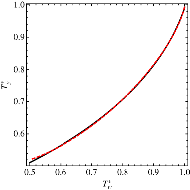
Figure 2: Reduced temperature of the attractive HCY fluid as a function of the reduced temperature of water in the saturation branch of the vapor-liquid coexistence curve. The red dashed line corresponds to data extracted from figure 1 and the continuous line corresponds to Eq. (17).

Now we address the question of whether the above information, namely Eq. (17), allows us to ‘predict’ the coexistence curve of real water in real units using the results of the HCY fluid shown in figure 1. The answer proceeds as follows. For any temperature $T_{w}$ on the real water vapor-liquid equilibrium curve we first determine the corresponding $T^{*}_{w}$ and then use Eq. (17) to obtain the corresponding $T^{*}_{Y}$. Next we multiply it by $T_{Yc}$ and derive the corresponding vaporization and condensation densities $\rho_{Yvap}$ and $\rho_{Ycond}$. Finally the real densities are simply $\rho_{wt}\rho_{Yvap}/\rho_{Yt}$ and $\rho_{wt}\rho_{Ycond}/\rho_{Yt}$. Schematically if we denote by $f(T_{Y},z)$ the mapping which allows one to determine ($\rho_{Yvap}$, $\rho_{Ycond}$) in our approximation for the attractive HCY fluid, then the recipe to obtain the real water liquid-vapor equilibrium curve is:

$$(\rho_{wvap},\rho_{wcond})=\frac{\rho_{wt}}{\rho_{Yt}}f(F(T_{w}/T_{wc})T_{Yc},1.7118).$$ (18)

Figure 3 shows the predicted coexistence curve using this recipe and the real water coexistence curve. In this figure we have also included, for comparison, the results obtained from the TIP4P/2005 model.[16]

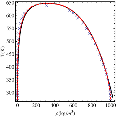
Figure 3: Liquid-vapor coexistence curve as obtained with the recipe (18) (dashed line), compared to experimental data[17] (continuous line) and the results of the TIP4P/2005 model[16] (crosses).

One can readily see the very good agreement between our prediction and the real coexistence curve, except close to the triple point. A particulary noteworthy feature is that Eq. (17) was derived by considering only the saturation branch, but it does a very good job also for the rest of the coexistence curve. Moreover, Eq. (17) admits the following appealing physical interpretation. Assume that, instead of considering a constant depth of the potential well at $r=\sigma$ (as we have done so far with $\epsilon=\epsilon_{c}$), in order to make the HCY fluid thermodynamically equivalent to real water for each temperature $T$ we are taking an effective HCY potential with the same $\sigma$ and $z$ but with $\epsilon\equiv\epsilon(T)$. Then, Eq. (16) can be rewritten as

$$\frac{T/\epsilon(T)}{T_{c}/\epsilon_{c}}=F\left(\frac{T}{T_{c}}\right).$$ (19)

or, equivalently,

$$\epsilon(T)=\epsilon_{c}\frac{T}{T_{c}F(T/T_{c})}$$ (20)

In figures 4 and 5 we show the effective (temperature dependent) potential as a function of distance and the temperature dependence of its depth at $r=\sigma$, respectively. Note that the overall shape of the potential is preserved, but the effect of the extra (non monotonous) temperature dependence of $\epsilon$ on the coexistence curve is clearly important. Although such a task lies beyond the scope of the present paper, we are persuaded that it would be interesting to investigate whether this effective interaction may provide an adequate picture of the real interaction between water molecules.

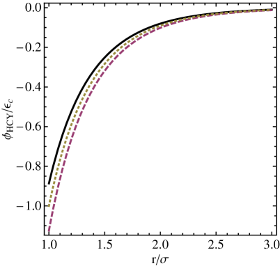
Figure 4: Effective (temperature dependent) attractive HCY potential as a function of distance for different temperatures: Continuous line: $T=273\ K$; dashed line: $473\ K$; dotted line: $647\ K$.

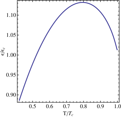
Figure 5: Temperature dependence of the well depth $\epsilon(T)$ as given by Eq. (20).

The next question that comes to mind is whether the same scaling of the temperature and density will hold for the equation of state. This is examined in the next subsection.

3.3 The equation of state of liquid water

The explicit form for our approximation to the attractive HCY fluid equation of state is given in Eq. (15) but, with the above discussion, it will be understood that we shall use in it the temperature dependent $\epsilon(T)$ as given by Eq. (19). However, one finds that the critical pressure obtained in this way with the attractive HCY fluid is $P_{Yc}=38.08$ MPa whereas the real critical pressure is $P_{wc}=22.064$ MPa. This overestimation seems to be due to a similar feature observed for the results derived within the thermodynamic perturbation theory for the attractive HCY fluid. In fact, in reference [9] we pointed out that the predicted critical pressure for the attractive HCY fluid was always greater than simulation values. For instance, if $z=1.8$ (which is the value of the inverse range parameter closest to our $z=1.7118$ here where simulation results are available), the critical pressure obtained from Eq. (15) is $\bar{P}=0.1576$ whereas from simulations one gets approximately $\bar{P}=0.101$ [20]. This gives a ratio $0.101/0.1576=0.6409$. In the present case, the ratio $P_{wc}/P_{Yc}$ yields $\gamma=22.064/38.08=0.5794$ which could be reasonably attributed to the discrepancy between the predicted critical pressure of the attractive HCY fluid and the value that one would obtain from simulation $z=1.7118$. Hence, we ‘correct’ our equation of state Eq. (15) with a factor $\gamma=22.064/38.08=0.5794$ so that it now reads

$$P=\gamma\left[\rho k_{B}TZ_{{HS}}(\frac{\pi}{6}\rho\sigma^{3})-2\pi{\rho}^{2}\sigma^{3}\epsilon(T)e^{z}\frac{\partial}{\partial\rho}\left(\rho G(z)\right)\right].$$ (21)

Figure 6 shows the result of using Eq. (21) together with the experimental isotherms[17] and those that follow from the Jeffery-Austin equation of state [6]. Clearly the agreement between this corrected equation of state and the experimental data for the isotherms is reasonably good in the liquid region except close to the critical and triple point isotherms. In the case of the critical isotherm, it leads to the correct critical point but deviates from the real critical isotherm at higher densities. On the other hand, the Jeffery-Austin results are also remarkably accurate, but show similar limitations. In particular they fail to produce the correct critical isotherm.

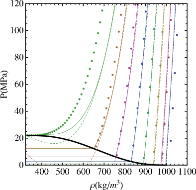
Figure 6: Isotherms as obtained from experimental data[17] (continuous lines), from Eq. (21) (dots) and from the Jeffery-Austin equation of state[6] (dashed lines). From right to left the curves correspond to $T=300$ K, $T=350$ K, $T=400$ K, $T=450$ K, $T=500$ K, $T=550$, K $T=600$ K and $T=T_{wc}$. The real coexistence line has been drawn to clearly indicate the liquid phase region.

4 Vapor-liquid equilibrium lines in the $P-T$ and $P-\rho$ planes.

Once we have shown that the real vapor-liquid equilibrium coexistence curve may be accurately described in the $T$-$\rho$ plane through the use of our approximate (corrected) equation of state, Eq. (21), it is reasonable to wonder if using the same approximate equation of state one may get also an accurate description in the $P-T$ and $P-\rho$ planes. The answer to the above question is only partially affirmative in the sense that the approximation is very rough. In order to get an accurate description one is forced to make a subsequent rescaling on the pressure which, in this instance, is unfortunately not simple due to the form of the relationship between the reduced real pressure ($P_{w}^{*}=P_{w}/P_{wc}$) and the reduced HCY pressure ($P^{*}_{y}=\bar{P}_{y}/\bar{P}_{yc}$) derived from the coexistence curves in the $P-T$ plane and given by the curve in figure 7.

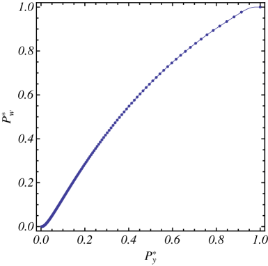
Figure 7: Relationship between the reduced pressures of the real water and of the HCY fluid as derived from the coexistence curves in the $P-T$ plane. The continuous line is the fit given in Eq. (22)

In order to fit accurately this curve both in the low pressure end and close to the critical pressure it is unavoidable to introduce a high order polynomial. We have taken the following form:

$$P^{{}^{\prime}}(P)=\sum_{i=1}^{14}c_{i}P^{i},$$ (22)

where the coefficients $c_{i}$ are given by $c_{1}=-0.149421$, $c_{2}=1.91855$, $c_{3}=-1.23117$, $c_{4}=0.519336$, $c_{5}=-0.150666$, $c_{6}=0.0306816$, $c_{7}=-0.004456$, $c_{8}=0.000466$, $c_{9}=-0.000035$, $c_{10}=1.880416\times 10^{-6}$, $c_{11}=-7.003285\times 10^{-8}$, $c_{12}=1.719548\times 10^{-9}$, $c_{13}=-2.501064\times 10^{-11}$ and $c_{14}=1.631257\times 10^{-13}$.

In figure 8, we show in a log-linear plot the comparison between the different coexistence curves in the $P$-$T$ plane. Note the disagreement between the experimental curve and the one obtained with the attractive HCY fluid using only Eq. (21) and the substantial improvement once the scaling implied by Eq. (22) is introduced. The inclusion of the results obtained with the TPI4P/2005 model[16] serves to indicate that the qualitative tendency is reproduced by this model but the pressure is underestimated.

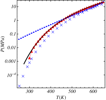
Figure 8: Coexistence curves in the $P$ -$T$ plane in a log-linear plot. Continuous line: experimental data[17]; dots: attractive HCY fluid with temperature rescaled using Eq. (17); triangles: attractive HCY fluid with temperature rescaled using Eq. (17) and pressure rescaled using Eq. (22); crosses: results from the TPI4P/2005 model[16].

Finally, we consider the $P-\rho$ plane. Figure 9 contains the comparison between the different coexistence curves in this plane. Note once more the disagreement between the experimental curve and the one obtained with the attractive HCY fluid using Eq. (21) and the improvement when the scaling given by Eq. (22) is also used. Again, the TPI4P/2005 model[5, 16] correctly reproduces the qualitative trends but in particular the critical pressure is highly underestimated.

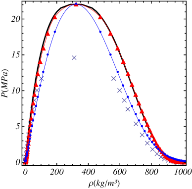
Figure 9: Coexistence curves in the $P$ - $\rho$ plane. Continuous line: experimental data[17]; dots: attractive HCY fluid with temperature rescaled using Eq. (17); triangles: attractive HCY fluid with temperature rescaled using Eq. (17) and pressure rescaled using Eq. (22); crosses: results from the TPI4P/2005 model[16].

5 Concluding remarks.

As the results of the previous section indicate, we have been able to use a simple model of intermolecular interaction, the attractive HCY fluid, to obtain a very reasonable picture of the thermodynamic behavior of water in the stable liquid phase. This is remarkable given the fact that the model does not consider at all important aspects such as bond geometry or charge distribution. In fact, our formulation involving an effective (temperature-dependent) attractive HCY interaction shares some aspects of the approach followed in colloidal systems, where some degrees of freedom are accounted for by an effective interaction potential. Moreover, the present development is yet another effort in devising a sound molecular theory of liquid water based on the principles of statistical mechanics and the thermodynamic perturbation theory of liquids. It is fair to say that with much less effort compared to the IAWPS Formulation 1995[3] and probably also to the Jeffery-Austin equation of state[6] we are able to achieve good accuracy. We should of course acknowledge the semiphenomenological character of our approach that allowed us to have this description, namely the fit of the inverse range parameter of the model $z$ and the manipulations involved in the various rescalings. Also worth mentioning in this regard is the limitation to the liquid phase, which becomes manifest in that the agreement between experimental data and our formulation gets worse both near the critical point and near the triple point. Furthermore, the scaling implied in Eq. (17) prevents us from dealing with the supercritical region which is of course interesting in many industrial processes. However, a similar procedure could be devised if one wanted to deal with the equation of state of steam. In such a case, instead of rescaling the temperature as we have done here, one could rescale the density. This might also lead to a density-dependent pair potential which could be analyzed following the recent approach introduced by Zhou [21], although the use of density-dependent pair potentials is not free from controversy [22]. Such developments lie beyond the scope of the present paper. Nevertheless, we seem to have been able to capture the main physics behind the thermodynamic properties of liquid water over a wide range of both temperatures and pressures. Therefore, and given the fact that the value of $z=1.7118$ that we used in our calculations is relatively close to the one ($z\simeq 2$) in which the thermodynamic properties of the attractive HCY are similar to those of the Lennard-Jones fluid, we wonder whether the replacement of the Lennard-Jones centers by attractive HCY centers in models used in simulation such as the TPI4P/2005 model[5] might improve the prediction say of the critical pressure. This may only be ascertained by performing the simulation and our hope is that, apart from the potential use by engineers of the above results, this work may find an echo in this latter respect.

Acknowledgments

We acknowledge the financial support of DGAPA-UNAM through project IN -109408-2. The work of M.L.H. has also been supported by the Ministerio de E- ducación y Ciencia (Spain) through Grant No. FIS2007-60977 (partially financed by Feder funds) and by the Junta de Extremadura through Grant No. GRU09038. We also want to thank A. Santos, C. Vega and J. V. Sengers for helpful comments.

References

- [1] See for instance A. Ben-Naim, Molecular Theory of Water and Aqueous Solutions. Part I: Understanding Water (World Scientific, Singapore, 2009); K. Szalewicz, C. Leforestier, and A. van der Avoird, Chem. Phys. Lett. 482, 1 (2009); F. Paesani and G. A. Voth, J. Phys. Chem. B 113, 5702(2009); C. Vega, J. L. F. Abascal, M. M. Conde and J. L. Aragones, Faraday Discuss. 141, 251 (2009); J. Jirsák and I. Nezbeda, J. Chem. Phys. 127, 124508 (2007); P. G. Debenedetti, J. Phys.: Condens. Matter 15, R1669 (2003); B. Guillot, J. Mol. Liq. 101, 219 (2002); J. L. Finney, J. Mol. Liq. 90, 303 (2001); I. Nezbeda, J. Mol. Liq. 73, 317 (1997); and references therein.
- [2] IAPWS Revised Release on the IAWPS Formulation 1995 for the Thermodynamic Properties of Ordinary Water Substance for General and Scientific Use (2009). Available from http://www.iawps.org .
- [3] W. Wagner and A. Pruss, J. Phys. Chem. Ref. Data 31, 387 (2002).
- [4] W. L. Jorgensen, J. Chandrasekhar, J. D. Madura, R. W. Impey and M. L.Klein, J. Chem. Phys. 79, 926 (1983).
- [5] J. L. F. Abascal and C. Vega, J. Chem. Phys. 123, 234505 (2005).
- [6] C. A. Jeffery and P. H. Austin, J. Chem. Phys. 110, 484 (1999).
- [7] G. Ihm, Y. Song and E. A. Mason, J. Chem. Phys. 94, 3839 (1990).
- [8] P. H. Poole, F. Sciortino, T. Grande, H. E. Stanley and C. A. Angell, Phys. Rev. Lett. 73, 1632 (1994).
- [9] M. Robles and M. López de Haro, J. Phys. Chem. C 111, 15957 (2007).
- [10] See for instance D. J. Naresh and J. K. Singh, Fluid Phase Equilibria 285, 36 (2009); Y. Kadiri, R. Albaki and J. L. Bretonnet, Chem. Phys. 352, 135 (2008); P. Orea and Y. Duda, J. Chem. Phys. 128, 134508 (2008) and references therein.
- [11] C. Vega, J. L. F. Abascal, E. Sanz, L. G. MacDowell and C. McBride, J. Phys.: Condens. Matter 17, S3283 (2005).
- [12] R. W. Zwanzig, J. Chem. Phys. 22, 1420 (1954).
- [13] M. López de Haro, S. Bravo Yuste, and A. Santos, “Alternative Approaches to the Equilibrium Properties of Hard-Sphere Liquids,” in Theory and Simulation of Hard-Sphere Fluids and Related Systems, edited by A. Mulero, Lect. Notes Phys. 753 (Springer, Berlin, 2008), pp. 183 – 245, and references therein.
- [14] N. F. Carnahan and K. E. Starling, J. Chem. Phys. 51, 635 (1969).
- [15] In the approximation for the equation of state of the attractive HCY fluid that we use here, the density at the triple point coincides with the freezing density of the HS fluid. The value we are using for this freezing density was taken from E. G. Noya, C. Vega, and E. de Miguel, J. Chem. Phys. 128, 154507 (2008).
- [16] C. Vega, J. L. F. Abascal, and I. Nezbeda, J. Chem. Phys. 125, 034503 (2006).
- [17] http://webbook.nist.gov/chemistry/fluid/
- [18] See for instance S. B. Kiselev, Fluid Phase Equilibria 147, 7 (1998); S. B. Kiselev and J. F. Ely, Fluid Phase Equilibria 222–223, 149 (2004); J. Wang and M. A. Anisimov, Phys. Rev. E 75 051107 (2007).
- [19] F. Llovel, L. F. Vega, D. Seiltgens, A Mejía, and H. Segura, Fluid Phase Equilibria 264, 201 (2008).
- [20] K. P. Shukla, J. Chem. Phys., 112, 10358 (2000).
- [21] S. Zhou, J. Chem. Phys., 128, 104511 (2008).
- [22] A. A. Louis, J. Phys.: Condens. Matter 14, 9187 (2002); C. F. Tejero, J. Phys.: Condens. Matter 15, S395 (2003)