Colder and Hotter: Interferometric imaging of $\beta$ Cassiopeiae and $\alpha$ Leonis

Abstract

Near-infrared interferometers have recently imaged a number of rapidly rotating A-type stars, finding levels of gravity darkening inconsistent with theoretical expectations. Here, we present new imaging of both a cooler star $\beta$ Cas (F2IV) and a hotter one  $\alpha$ Leo (B7V) using the CHARA array and the MIRC instrument at the H band. Adopting a solid-body rotation model with a simple gravity darkening prescription, we modeled the stellar geometric properties and surface temperature distributions, confirming both stars are rapidly rotating and show gravity darkening anomalies. We estimate the masses and ages of these rapid rotators on $\emph{L-R}_{\rm{pol}}$ and HR diagrams constructed for non-rotating stars by tracking their non-rotating equivalents. The unexpected fast rotation of the evolved sub-giant $\beta$ Cas offers a unique test of the stellar core-envelope coupling, revealing quite efficient coupling over the past $\sim$ 0.5  Gyr. Lastly we summarize all our interferometric determinations of the gravity darkening coefficient for rapid rotators, finding none match the expectations from the widely used von Zeipel gravity darkening laws. Since the conditions of the von Zeipel law are known to be violated for rapidly rotating stars, we recommend using the empirically-derived $\beta$ = 0.19 for such stars with radiation-dominated envelopes. Furthermore, we note that no paradigm exists for self-consistently modeling heavily gravity-darkened stars that show hot radiative poles with cool convective equators.

1 Introduction

Stellar rotation is a fundamental property of stars in addition to the mass and metallicity. However it has been generally overlooked in the past century for mainly three reasons. Firstly, most stars rotate slowly. Secondly, no complete stellar rotational model is available to handle the stellar structure and evolution of a rotating star. Thirdly, although stellar rotational velocities in the line of sight $v\sin i$  are relatively easy to measure, the inclination angles are generally unknown, leaving large uncertainties of stellar rotational velocities.

While almost all cool stars rotate slowly, rapid rotation is the norm for hot stars. A large fraction of hot stars are observed to be rotating with equatorial velocities larger than 120  km s^-1 (Abt & Morrell, 1995; Abt et al., 2002). Such fast stellar rotation can have strong effects on the observed stellar properties. The strong centrifugal forces distort stellar shapes and make them oblate. Stellar surface temperatures vary across latitudes due to the gravity darkening (von Zeipel, 1924a, b). Lower effective gravity at the equator result in lower temperatures compared to the poles. This temperature distribution implies that apparent luminosities $\emph{L}_{\mathrm{app}}$ and apparent effective temperatures $\emph{T}_{\mathrm{app}}^{\mathrm{eff}}$ depend on inclination angles, and the overall values are hidden from observers. Stellar rotation can also affect the distribution of chemical elements, mass loss rate and stellar evolution (Meynet & Maeder, 2000). Some kind of rapidly rotating massive stars may end up as $\gamma$-ray bursts (MacFadyen & Woosley, 1999).

Stellar rotation has been studied mainly through the Doppler broadening line profiles in the past, but the obtained information from these studies is limited due to the lack of spatial knowledge of stars, such as the inclination angles. An important and reliable way to extract such information is through long baseline optical/infrared interferometry, allowing us to study the detailed stellar surface properties for the first time. Several rapid rotators has been well studied using this techniques, including Altair, Vega, Achernar, Alderamin, Regulus and Rasalhague (van Belle et al., 2001, 2006; Aufdenberg et al., 2006; Peterson et al., 2006; Domiciano de Souza et al., 2003; Monnier et al., 2007; Zhao et al., 2009).

These studies have revealed not only the stellar surface geometry but also the surface temperature distributions, allowing us to test and constrain stellar models and laws. For instance, the surface temperature distributions have confirmed the gravity-darkening law in general, but deviate in detail from the standard von Zeipel model ($\emph{T}_{\mathrm{eff}}$ $\propto$ $\emph{g}_{\mathrm{eff}}^{\rm{\beta}}$, where $\beta$ = 0.25 for fully radiative envelopes). Particularly the studies on Altair and Alderamin prefer non-standard $\beta$ values from the modified von Zeipel model (the $\beta$-free model in Zhao et al. (2009)). These results imply the gravity darkening law is probably only an approximation of the surface temperature distribution, the real physics behind is still to be uncovered.

In this paper we show our studies of two rapidly rotating stars with extreme spectral types in contrast to all the A type stars we have studied: $\beta$ Cassiopeiae and $\alpha$ Leonis, observed with the Center for High Angular Resolution Astronomy (CHARA) long baseline optical/IR interferometry array and the Michigan Infra-Red Combiner (MIRC) beam combiner. $\beta$ Cassiopeiae ($\beta$ Cas, Caph, HR21) has V = 2.27, (Morel & Magnenat, 1978), H = 1.584 (Cutri et al., 2003), 1.43 (Ducati, 2002), and is located at d = 16.8 pc (van Leeuwen, 2007). Its mass has been estimated as 2.09  M_⊙(Holmberg et al., 2007, see the electronic table on VizieR) and it has been classified as F2III-IV (Rhee et al., 2007), implying it was an A type star during main sequence and has evolved – here we will present updated mass and luminosity estimates (see Section 5). The rotational velocity has been reported between $v\sin i$  = 69  km s^-1 (Glebocki & Stawikowski, 2000) and 82  km s^-1 (Bernacca & Perinotto, 1970) in the literature, although recent measurements are more consistently confined from 69  km s^-1 to 71  km s^-1 (Glebocki & Stawikowski, 2000; Reiners, 2006; Rachford & Foight, 2009; Schröder et al., 2009) which we prefer to use in this paper. Previous studies measured its apparent effective temperature range from 6877 Kto 7200 K(Gray et al., 2001; Daszyńska & Cugier, 2003; Rhee et al., 2007; Rachford & Foight, 2009) and estimated its radius from 3.43  R_⊙to 3.69  R_⊙(Richichi & Percheron, 2002; Daszyńska & Cugier, 2003; Rachford & Foight, 2009).

$\alpha$ Leonis (Regulus, HR3982) has V = 1.391 (Kharchenko et al., 2009), H = 1.658 (Cutri et al., 2003), 1.57 (Ducati, 2002), distance d = 24.31 pc (van Leeuwen, 2007). It is a well-known rapidly rotating star, classified as a B7V star (Johnson & Morgan, 1953) or B8 IVn (Gray et al., 2003). The $v\sin i$  measurements from the literature spread a large range from $\sim$ 250  km s^-1 (Stoeckley et al., 1984) to $\sim$ 350  km s^-1 (Slettebak, 1963) and we have adopted here the recent precise value 317 $\pm$ 3  km s^-1 from McAlister et al. (2005). Regulus is also a famous triple star system with the companions B and C forming a binary system at $\sim$ 175” away from $\alpha$ Leonis A (McAlister et al., 2005). Recently Gies et al. (2008) discovered that $\alpha$ Leonis A is also a spectroscopic binary with a white dwarf company ($\sim$ 0.3  M_⊙) of the orbital period $\sim$ 40.11 d. The primary mass has been estimated $\sim$ 3.4  M_⊙(McAlister et al., 2005), however our study here will show it is much more massive. The diameter of Regulus has been estimated several times in the past because of its brightness and relatively large angular size. McAlister et al. (2005) combined the CHARA K-band interferometric data and a number of constraints from spectroscopy and revealed that Regulus has the polar radius R_pol = 3.14 $\pm$ 0.06  R_⊙and the equatorial radius R_eq = 4.16 $\pm$ 0.08  R_⊙.

In this paper, we describe the observations and data reduction in Section 2. Then we show the results of $\beta$ Cas and $\alpha$ Leo from both the standard and modified von Zeipel models in Section 3. In Section 4, we present aperture synthesis images. In Section 5, the locations of the two rapid rotators on $\emph{L-R}_{\rm{pol}}$ and HR diagrams are discussed. We consider the coupling of the stellar core to the outer envelope and explore gravity darkening from studying these two rapid rotators in Section 6. We conclude in Section 7.

2 Observation And Data Reduction

The observations were carried out at the Georgia State University (GSU) Center for High Angular Resolution Astronomy (CHARA) interferometer array located on Mt. Wilson. The CHARA array includes six 1-meter telescopes which are arranged in a Y shape configuration: two telescopes in each branch. It can potentially provide 15 baselines simultaneously ranging from 34  m to 331  m, possessing the longest baselines in optical/IR of any facility. With these baselines, CHARA offers high angular resolution up to $\sim$0.4  mas at the H band and $\sim 0.7$  mas at the K band.

The Michigan Infra-Red Combiner (MIRC) is designed to perform true interferometric imaging. It is an image plane combiner, combining 4 CHARA telescopes simultaneously to provide 6 visibilities, 4 closure phases and 4 triple amplitudes. Currently MIRC is mainly used in H band which is further dispersed by a pair of prisms into 8 narrow channels. In order to obtain stable measurements of visibility and closure phase, MIRC utilizes single-mode fibers to spatially filter out the atmosphere turbulence. The fibers are arranged on a v-groove array with a non-redundant pattern so that each fringe has a unique spatial frequency signature. The beams exiting the fibers are collimated by a microlens array and then focused by a spherical mirror to interfere with each other. Since the interference fringes only form in one dimension which is parallel to the v-groove, they are compressed and focused by a cylindrical lens in the dimension perpendicular to the v-groove to go through a slit of a spectrograph. The data presented here utilized a pair of low spectral resolution prisms with R $\sim$ 50. Finally the dispersed fringes are detected by a PICNIC camera (Monnier et al., 2004, 2006). The philosophy of the control system and software is to acquire the maximum data readout rates in real time. The details about the software can be found in Pedretti et al. (2009).

The integration time is limited by the fast changing turbulence, any turbulence faster than 3.5 ms readout speed of the camera will cause decoherence of the fringes. In order to calibrate these fringes, calibrators with known sizes adjacent to the targets are observed each night. For the acquisition of true visibility, real time flux of the beam from each telescope is also required. Several independent methods (Fiber, Chopper and DAQ , Monnier et al. (2008)) are adopted to indirectly measure the ’real time’ flux. A recent upgrade of MIRC with Photometric Channels has been achieved to directly and more accurately measure the flux. Photometric Channels place a beamsplitter right after the microlens array to reflect $\sim$ 25% of the flux into multi-mode fibers. The beams exiting the MM fibers go through the same doublet and prisms, and hit a different quadrant of the same detector. With Photometric Channels MIRC can now measure the visibilities with uncertainty down to 3% (Che et al., 2010).

We observed $\beta$ Cas on 7 nights in 2007 and 2009, and $\alpha$ Leo on 5 nights in 2008. The detailed log is presented in Table 1. Figure 1 shows the overall (u,v) baseline coverage of the observation of $\beta$ Cas and $\alpha$ Leo .

Table 1: Observation logs for $\beta$ Cas and $\alpha$ Leo 

Target	Obs. Date	Telescopes	Calibrators
$\beta$ Cas	UT 2007Aug07	S1-E1-W1-W2	7 And
	UT 2007Aug08	S1-E1-W1-W2	$\sigma$ Cyg, 7 And
	UT 2007Aug10	S1-E1-W1-W2	$\sigma$ Cyg, 37 And
	UT 2007Aug13	S1-E1-W1-W2	$\sigma$ Cyg, 7 And, Ups And
	UT 2009Aug11	S1-E1-W1-W2	7 And, $\gamma$ Tri
	UT 2009Aug12	S1-E1-W1-W2	7 And, $\gamma$ Tri
	UT 2009Oct22	S2-E1-W1-W2	37 And, $\upsilon$ And, $\epsilon$ Cas, $\eta$ Aur
$\alpha$ Leo	UT 2008Dec03	S1-E1-W1-W2	$\theta$ Leo
	UT 2008Dec04	S1-E1-W1-W2	54 Gem, $\eta$ Leo
	UT 2008Dec05	S1-E1-W1-W2	$\theta$ Hya, $\theta$ Leo
	UT 2008Dec06	S1-E1-W1-W2	54 Gem, $\theta$ Hya, $\eta$ Leo
	UT 2008Dec08	S1-E1-W1-W2	$\theta$ Leo

…..

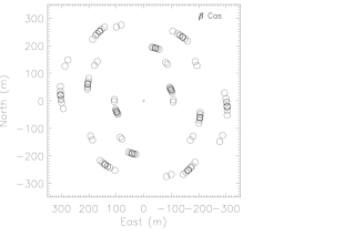
Figure 1: Baseline coverage of the all nights observation of $\beta$ Cas and $\alpha$ Leo . UV coverage can be calculated by dividing these baselines by the wavelength of H band channels.

Monnier et al. (2007) describes the data reduction pipeline used to process the data, which was validated by using data on the calibration binary $\iota$ Peg. The pipeline first computes uncalibrated squared-visibilities and complex triple amplitudes after a series of background subtractions, Fourier transformations and foreground subtractions. Then the uncalibrated squared-visibilities and complex triple amplitudes are calibrated by the fluxes measured simultaneously with fringes. The calibrators with known sizes are observed to compensate for the system visibility drift, as listed in Table 2.

Table 2: Calibrator diameters

Calibrator	UD diameter ( mas)	Reference
7 And	0.659 $\pm$ 0.017	b, c, d
37 And	0.682 $\pm$ 0.030	b, c
$\upsilon$ And	1.14 $\pm$ 0.007	a, b, c, d
$\sigma$ Cyg	0.542 $\pm$ 0.021	a
$\gamma$ Tri	0.520 $\pm$ 0.0125	b
$\epsilon$ Cas	0.351 $\pm$ 0.024	c, d
$\eta$ Aur	0.419 $\pm$ 0.063	c
$\theta$ Leo	0.678 $\pm$ 0.062	b, c
$\eta$ Leo	0.644 $\pm$ 0.068	c
54 Gem	0.735 $\pm$ 0.033	b, c
$\theta$ Hya	0.463 $\pm$ 0.031	c, d

3 Modeling of Rapid Rotators

We construct a 2D stellar surface model in this paper: the modified von Zeipel model. The model contains six free parameters, stellar polar radius, the polar temperature, the ratio of angular velocity to critical speed $\omega$ / $\omega_{\rm crit}$, the gravity darkening coefficient ($\beta$), the inclination angle, and the position angle (east of north) of the pole, to describe the stellar radius, surface effective gravity and temperature distributions across stellar surface. The mass of a star is given and fixed in each model fitting process. Given the stellar mass, stellar polar radius and $\omega$ / $\omega_{\rm crit}$, the stellar radius and surface effective gravity at each latitude can be determined (Aufdenberg et al., 2006). Then given the stellar polar temperature and $\beta$, the stellar surface temperature distribution can be computed from the gravity darkening law(T $\propto$ $\emph{g}_{\mathrm{eff}}^{\rm{\beta}}$). Lastly the orientation of the star is described by the inclination angle and position angle. In the model, we assume the solid-body rotation for simplicity; a more complicated and realistic model would consider the differential rotation which requires additional information (such as spectral lines) for fitting. The gravity darkening coefficient $\beta$ is a free parameter in the model. By fixing $\beta$, the model reduces to the standard von Zeipel model ($\beta$ = 0.25, radiative case) or Lucy model ($\beta$ = 0.08, convective case).

In earlier work (Monnier et al., 2007), we found that allow $\beta$ to be a free parameter greatly improved the fit to the interferometric data. This flexibility allows us to independently test the validity of the standard von Zeipel and Lucy prescriptions. Furthermore, the mixture of radiative and convective regions in the same star may also cause deviations from expected values. For example, the polar temperature could be thousands of degrees higher than the equator temperature, resulting in a situation where upper atmosphere may be radiative at the poles while convective at the equator. In general, the value of $\beta$ also depends on various approximations made for the atmosphere, radiation transfer etc. (Claret, 1998). Therefore in our modified von Zeipel model, instead of setting $\beta$ to be fixed, we allow $\beta$ to change as a single free parameter of the model to fit the interferometric data. For comparison, we also present models with $\beta$ fixed to the appropriate standard value. The error bars of stellar parameters from the modified von Zeipel model are in general larger than those from standard von Zeipel model or Lucy model. This is because there are certain degrees of degeneracies between the gravity darkening coefficient $\beta$ and other stellar parameters, as discussed below.

During the model fitting process, the modified von Zeipel model is converted into a projected stellar surface brightness model, which is constrained by the observed V and H band photometric fluxes and three kinds of interferometric data from each night: squared visibilities, closure phases and triple amplitudes. In the modified von Zeipel model, the stellar surface is divided into small patches. The intensity of each patch is computed from Kurucz model (Kurucz, 1992) given the temperature, gravity, viewing angle and wavelength, so that the modified von Zeipel model can be converted into the projected brightness model. The projected brightness model is then converted into the same three kinds of interferometric data above by direct Fourier transform to fit to the observed data. We use 4 sub-bands (binning two adjacent narrow channels dispersed by the MIRC prisms) across H band for accuracy. In addition, the apparent V and H band photometric fluxes are obtained from the projected brightness model to fit to the observed values. Observed $v\sin i$  is not directly used in the model fitting, but used to cross-check the results from model fitting. The detailed process is described in Zhao et al. (2009) and reference therein.

Data errors consist of random errors, errors due to variation of seeing condition, and calibration errors from using incorrect diameters of the calibrator targets. To get the errors from the first two parts, we treat the data from each night as a whole package and bootstrap packages randomly with replacement. Then we fit the sampled data and repeat fifty times to get the distribution of each model parameter. The upper and lower error bars quoted here are such that the interval contains 68.3% probability and the probability above and below the interval are equal. For the error from the third part, we used simple Monte Carlo sampling using the our estimated angular size uncertainties – these errors turned out to be somewhat smaller than the error from the first two parts.

We should point out that the stellar mass has to be given and fixed at the beginning of each model fitting process, but at first does not agree in detail with the model estimated from the fitting results on both $\emph{L-R}_{\rm{pol}}$ and HR diagrams using the rotational correction (see Section 5). Our approach here has been to adopt the mass from the literature for the first attempt in the model fitting. The mass estimation from the first attempt is then used in the second round of model fitting process. This procedure is repeated until the mass given in the model agrees with what comes out of the model fitting. The final mass is referred as the model mass in our paper. The stellar metallicities are adopted from the literature and fixed throughout. The distances of the targets are also adopted from the literature.

We also calculate the stellar mass based on the measured $v\sin i$  range from the literature, which is referred as the oblateness mass and was first proposed by Zhao et al. (2009). For each bootstrap, we extract the inclination angle, polar radius and $\omega$ / $\omega_{\rm crit}$ from the best fitting, then uniformly sample $v\sin i$  values 100 times in the given range to obtain a mass distribution. By combining the mass distribution from each bootstrap, we obtain the whole mass distribution from which the upper and lower mass bound can be calculated such that the interval contains 68.3% probability and the probability above the upper bound and below the lower bound are the same. To compute the best estimation of the stellar mass, we use the best estimations of the inclination angle, polar radius and $\omega$ / $\omega_{\rm crit}$ from the model fitting of all nights, and the $v\sin i$  value to be the mean of the measured range from the literature.

3.1 $\beta$ Cassiopeiae

We adopted the following basic properties of $\beta$ Cas from the literature as inputs: distance = 16.8 pc(van Leeuwen, 2007) and metallicity [Fe/H] = 0.03 (Gray et al., 2001). We take [Fe/H] = 0 which is the closest value to the observation to extract intensities from Kurucz model. M = 2.09 M_⊙ (Holmberg et al., 2007, see the electronic table on VizieR) is adopted for the first attempt of the model fitting. The fitting results and final parameters from the modified von Zeipel model are shown in Fig. 10 in the Appendix and the middle column of Table 3 respectively. The results show that $\beta$ Cas is rotating more than 90% of its critical rate, which causes its radius $\sim$ 24% longer at the equator than at the poles. The temperature at the pole is about 1000 K higher than that at the equator. These significant differences between the poles and equator imply that the $\emph{L}_{\mathrm{app}}$ and $\emph{T}_{\mathrm{app}}^{\mathrm{eff}}$ are highly dependent on viewing angles. The best model mass estimation of its non-rotating equivalent from $\emph{L-R}_{\rm{pol}}$ and HR diagrams is 1.91 M_⊙(Fig. 6), lower than 2.09 M_⊙from Holmberg et al. (2007). The oblateness mass estimation from $v\sin i$  range 69  km s^-1 to 71  km s^-1 is $1.77^{+0.17}_{-0.05}$ M_⊙, which is consistent with our model mass within the error bars. $\beta=0.146$ from the modified von Zeipel model fitting is significantly different from standard values for either radiation-dominated or convection-dominated envelopes. The inclination angle is low, implying we are looking at more the polar area than the equatorial area as shown in Figure 4 (see Section 4). This is why the apparent luminosity $\emph{L}_{\mathrm{app}}$ is higher than $\emph{L}_{\mathrm{bol}}$ .

Claret (2000) has computed the evolution of gravity darkening coefficients for different stellar masses, and showed that at such low $\emph{T}_{\mathrm{eff}}$  as $\beta$ Cas it should be convection-dominated in the envelope. Fixing gravity darkening coefficient $\beta=0.08$ (Lucy model) for convective envelopes, we run model fitting again and the results are shown in the right column of Table 3. The best fitting $\chi^{2}$s for this model is much worse, nearly a factor of 2 higher. Many parameters from the Lucy model are similar to those from the modified von Zeipel model, except the temperature at the equator. This is not surprising because the low $\beta$ value means the weak dependence of the temperature on gravity, namely the temperature at the equator will be closer to that at the poles for the Lucy model. Consequently the luminosities and temperature $\emph{L}_{\mathrm{app}}$ , $\emph{L}_{\mathrm{bol}}$ and $\emph{T}_{\mathrm{app}}^{\mathrm{eff}}$ are a little higher than those from the modified von Zeipel model. The modified von Zeipel model gives significantly lower $\chi^{2}$ than the Lucy model, especially that from the closure phase data which is sensitive to asymmetric structures on the stellar surface. This implies the modified von Zeipel model describes the surface temperature distribution better, ruling out the Lucy model in this case. This is also confirmed by comparing the model $v\sin i$  with the observed values: $v\sin i$  = $72.4^{+1.5}_{-3.5}$  km s^-1 from the modified von Zeipel model agrees with the observation 69  km s^-1 to 71  km s^-1 , while from the Lucy model $v\sin i$  = $81.3^{+0.9}_{-1.0}$  km s^-1 deviates strongly from the observation. Further more, the oblateness mass and model mass don’t agree with each other, suggesting that the Lucy model is not self-consistent in this case.

We found that the low inclination angle induces strong degeneracies between some parameters during the model fitting. For example when a star is pole-on the darkness at the equator could be due to either the high angular velocity or the high gravitational darkening coefficient since the oblateness can not be directly constrained from this viewing angle. Therefore we explore the probability spaces of gravity darkening coefficients $\beta$ with inclination angles and $\omega$ / $\omega_{\rm crit}$ to assess possible correlations. For example, we first search the best model fitting results of all nights on a 40 $\times$ 40 grid of $\beta$ and inclinations by fixing these two parameters on each pixel. Generally if these two parameters are independent, then the probability of their true values falling into each pixel is $\propto$ $e^{-0.5\chi^{2}}$. However in this case the two parameters are dependent, we modify the probability $\propto$ $e^{-\alpha\chi^{2}}$, where $\alpha$ is a variable to be determined. Then we overplot the results of the two parameters from each bootstrap onto the probability space (not shown in the figure), and find the contour of the same $\chi^{2}$ containing 68.3% of bootstrap results, from which $\alpha$ can be computed. The contour is defined as 1-$\sigma$.

The left panel of Fig. 2 shows the degeneracy between $\beta$ and the inclination. The contour represents the 68.3% probability level, and is weakly elongated in one direction. We further overplot onto the probability space the observed $v\sin i$  range which intersects the contour. This means a precise $v\sin i$  measurement would significantly constrain the stellar parameters from our model fitting. The same idea is applied to the probability space of $\beta$ and $\omega$ / $\omega_{\rm crit}$ (Figure 2 right) which shows a stronger correlation between these two parameters.

…..

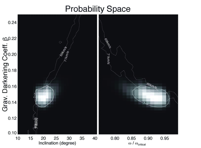
Figure 2: Probability spaces of $\beta$ Cas show the degeneracy between stellar parameters. The left panel shows the probability space of the gravity darkening coefficient $\beta$ and the inclination angle; the right one shows that of $\beta$ and the fraction of critical angular velocity $\omega$ / $\omega_{\rm crit}$. The solid contours represent the 1-$\sigma$ levels, containing 68.3% of the probability. And the dashed lines connect pixels in the probability space with the same $v\sin i$  values from model fitting. The value range 69  km s^-1 to 71  km s^-1 is adopted from the literature, and the corresponding lines intersect the 1-$\sigma$ contours. Both panels show the elongation of the contours, which imply some degeneracies between these parameters.

Table 3: Best-fit and physical parameters of $\beta$ Cas 

Model Parameters	Modified von Zeipel model ($\beta$-free)	Lucy model ($\beta$ = 0.08)
Inclination (degs)	$19.9^{+1.9}_{-1.9}$	$21.4^{+3.1}_{-0.9}$
Position Angle (degs)	$-7.09^{+2.24}_{-2.40}$	$-1.8^{+0.8}_{-1.7}$
Tpol ( K)	$7208^{+42}_{-24}$	$7108^{+14}_{-18}$
Rpol ( mas)	$0.849^{+0.023}_{-0.020}$	$0.835^{+0.035}_{-0.010}$
$\omega$ / $\omega_{\rm crit}$	$0.920^{+0.024}_{-0.034}$	$0.930^{0.011}_{-0.050}$
$\beta$	$0.146^{+0.013}_{-0.007}$	0.08 (fixed)
Derived Physical Parameters
Teq ( K)	$6167^{+36}_{-21}$	$6487^{+12}_{-17}$
Req ( R⊙)	$3.79^{+0.10}_{-0.09}$	$3.77^{+0.16}_{-0.04}$
Rpol ( R⊙)	$3.06^{+0.08}_{-0.07}$	$3.01^{+0.13}_{-0.04}$
Bolometric luminosity $\emph{L}_{\mathrm{bol}}$ ( L⊙)	$21.3^{+1.0}_{-0.7}$	$22.7^{+1.4}_{-0.3}$
Apparent effective temperature $\emph{T}_{\mathrm{app}}^{\mathrm{eff}}$ ( K)	6825	6897
Apparent luminosity $\emph{L}_{\mathrm{app}}$ ( L⊙)	27.3	28.3
Model $v\sin i$  ( km s-1 )	$72.4^{+1.5}_{-3.5}$	$79.8^{+0.9}_{-1.0}$
Rotation rate (rot/day)	$1.12^{+0.03}_{-0.04}$	$1.16^{+0.01}_{-0.06}$
Model mass ( M⊙)	$1.91\pm 0.02$	$1.95\pm 0.03$
Oblateness mass ( M⊙)	$1.77^{+0.17}_{-0.05}$	$1.45^{+0.12}_{-0.27}$
Age (Gyrs)	$1.18\pm 0.05$	$1.09\pm 0.03$
Model V Magnitude	$2.284^{+0.012}_{-0.019}$	$2.251^{+0.020}_{-0.006}$
Model H Magnitude	$1.398^{+0.007}_{-0.007}$	$1.394^{+0.010}_{-0.001}$
$\chi^{2}$ of various data
Total $\chi^{2}_{\nu}$	1.36	2.53
Vis2 $\chi^{2}_{\nu}$	1.26	1.56
CP $\chi^{2}_{\nu}$	2.18	4.81
T3amp $\chi^{2}_{\nu}$	0.45	0.60
Physical Parameters from the literature
[Fe/H]	0.03
Distance (pc)	16.8

3.2 $\alpha$ Leonis

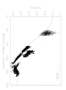
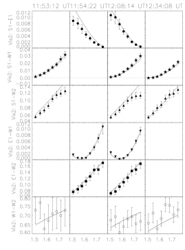
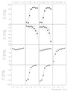
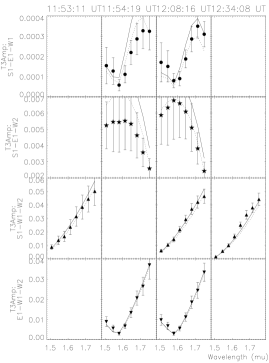
Figure 11: The similar panels of $\alpha$ Leo as those of $\beta$ Cas in Fig. 10. The reduced $\chi^{2}$ of model is 1.32 and that of image is 0.78.

We first fit the stellar surface of the modified von Zeipel model to the interferometric data of $\alpha$ Leo . The parameters we adopted from the literature are given as following: distance = 24.31 pc (van Leeuwen, 2007), metallicity [Fe/H] = 0.0 (Gray et al., 2003). Mass = 3.4  M_⊙(McAlister et al., 2005) was used for the first attempt of the model fitting. The fitting results from the modified von Zeipel model are shown in Fig. 11 in the appendix, with the final stellar parameters listed in the middle column of Table 4. $\alpha$ Leo is rotating at 96% of its critical speed, causing the equatorial radius about 30% longer than the polar radius. The temperatures at the poles are more than 3000K hotter than that at the equator. The gravitational darkening coefficient $\beta$ from the fitting is again different from the ”standard” values for either radiative or convective envelopes. The results show that $\alpha$ Leo is almost equator-on, which is shown as a dark strip in Figure 5 (see Section 4). Therefore the $\emph{L}_{\mathrm{bol}}$ is higher than the $\emph{L}_{\mathrm{app}}$ . The model mass from HR diagram is 4.15 $\pm$ 0.06  M_⊙. Adopting the $v\sin i$  range $v\sin i$  = 317 $\pm$ 3  km s^-1 from McAlister et al. (2005) paper, the oblateness mass estimation corresponding to the model mass is $3.66^{+0.79}_{-0.28}$ M_⊙, which also agrees with the model mass within the errors. The large errors of the oblateness mass is due to the degeneracy of stellar parameters as discussed later. The observed $v\sin i$  (McAlister et al., 2005) is consistent with our derived value $336^{+16}_{-24}$  km s^-1 with error bars.

Theoretically the high surface temperature of $\alpha$ Leo suggests that the envelope is fully radiative, corresponding to the gravity darkening coefficient $\beta=0.25$. We fit the model again using the fixed $\beta$ value, which is the standard von Zeipel model. The best fitting $\chi^{2}$s for this model is much worse, nearly a factor of 2 higher. For completeness, we have included the results in the right column of Table 4. In this scenario, $\alpha$ Leo is rotating even faster. The larger gravitational darkening coefficient and faster rotation imply even larger temperature difference between the poles and equator. However the derived equatorial temperatures from the modified and standard von Zeipel models agree with each other. This is because Regulus is almost equator-on, the observed interferometric data is dominated by information from the equator. The $\chi^{2}$s of the various interferometric data from the modified von Zeipel model are all significantly smaller than those from the standard von Zeipel model, supporting the modified von Zeipel model with $\beta$ = 0.19 is preferred to describe the surface properties of Regulus, ruling out the standard von Zeipel value. This conclusion is also supported by the disagreements between the model mass and oblateness mass from the standard von Zeipel model, and between the model and observed $v\sin i$  values (see Table 4).

We expect some degeneracies of parameters from the modified von Zeipel model fitting because of the symmetry of the equator-on orientation. Two figures of probability space of $\omega$ / $\omega_{\rm crit}$and the inclination vs. $\beta$ are shown in Figure 3. Both pictures show a strongly elongated contour of the probability, implying significant correlation between these parameters. The solid contours show the 68.3% probability. We overplot the observed $v\sin i$  range from McAlister et al. (2005), which intersects the contour with a much smaller common area. Therefore a precise $v\sin i$  measurement would significantly reduce the degeneracy between the parameters and constrain them much better.

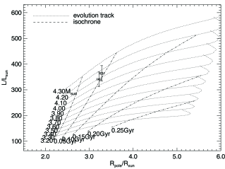
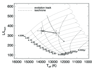
Figure 7: $\alpha$ Leo position on $\emph{L-R}_{\rm{pol}}$ and HR diagrams based on $Y^{2}$ model. The notations are the same as those on diagrams of $\beta$ Cas (see Fig. 6).

Based on only visibility data, McAlister et al. (2005) modeled $\alpha$ Leo and our new model results are generally consistent with this earlier work. Since MIRC has higher angular resolution, better UV coverage and the closure phase data, our data is more sensitive to the detailed structures such as the inclination and position angles. This work found acceptable fits for $\beta$ values between 0.12 and 0.34 (best fit at 0.25), a range consistent with our more refined analysis. Although our estimations of the bolometric luminosity $\emph{L}_{\mathrm{bol}}$ of Regulus is similar to those from their paper, the HR diagram (Fig. 7) from our results suggests that the mass of the non-rotating equivalent of Regulus is 4.15 $\pm$ 0.06 M_⊙, much more massive then the 3.4 $\pm$ 0.2 M_⊙that McAlister et al. (2005) obtained using the surface gravity $log~{}g$ from spectral analysis. Their results show that the non-rotating equivalent of Regulus has lower mass and consequently lower $\emph{L}_{\mathrm{bol}}$ than rapidly rotating Regulus, which is in contrast to what Sackmann (1970) found that a non-rotating equivalent actually has higher $\emph{L}_{\mathrm{bol}}$ than its rapidly rotating equivalent.

…..

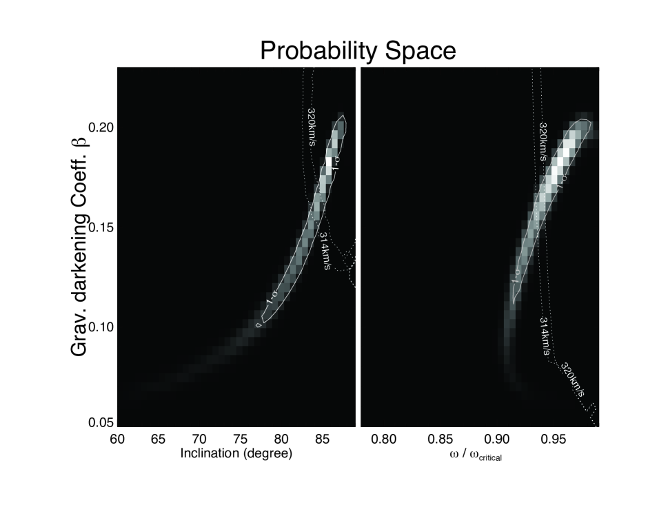
Figure 3: Probability spaces of $\alpha$ Leo show the degeneracy between stellar parameters. All the notations are the same as in the probability spaces of $\beta$ Cas (see Fig. 2). The strong elongation of the contours in both panels suggest strong correlation between these parameters. The dashed lines show the $v\sin i$  range from McAlister et al. (2005), which intersects the probability contours with smaller common areas.

Table 4: Best-fit and physical parameters of $\alpha$ Leo 

Model Parameters	Modified von Zeipel model ($\beta$-free)	von Zeipel model ($\beta$ = 0.25)
Inclination (degs)	$86.3^{+1.0}_{-1.6}$	$87.5^{+0.2}_{-0.1}$
Position Angle (degs)	$258^{+2}_{-1}$	$259^{+1}_{-2}$
Tpol ( K)	$14520^{+550}_{-690}$	$16190^{+150}_{-110}$
Rpol ( mas)	$0.617^{+0.010}_{-0.009}$	$0.605^{+0.001}_{-0.001}$
$\omega$ / $\omega_{\rm crit}$	$0.962^{+0.014}_{-0.026}$	$0.969^{+0.001}_{-0.002}$
$\beta$	$0.188^{+0.012}_{-0.029}$	0.25 (fixed)
Derived Physical Parameters
Teq ( K)	$11010^{+420}_{-520}$	$10920^{+100}_{-70}$
Req ( R⊙)	$4.21^{+0.07}_{-0.06}$	$4.17^{+0.007}_{-0.006}$
Rpol ( R⊙)	$3.22^{+0.05}_{-0.04}$	$3.16^{+0.005}_{-0.004}$
Bolometric luminosity $\emph{L}_{\mathrm{bol}}$ ( L⊙)	$341^{+27}_{-28}$	$431^{+18}_{-9}$
Apparent effective temperature $\emph{T}_{\mathrm{app}}^{\mathrm{eff}}$ ( K)	12080	12650
Apparent luminosity $\emph{L}_{\mathrm{app}}$ ( L⊙)	252	294
Model $v\sin i$  ( km s-1 )	$336^{+16}_{-24}$	$346^{+1}_{-2}$
Rotation rate (rot/day)	$1.64^{+0.02}_{-0.04}$	$1.70^{+0.01}_{-0.01}$
Model mass ( M⊙)	$4.15\pm 0.06$	$4.52\pm 0.05$
Oblateness mass ( M⊙)	$3.66^{+0.79}_{-0.28}$	$3.44^{+0.08}_{-0.01}$
Age ( Gyr)	$0.09\pm 0.02$	$0.05\pm 0.01$
Model V Magnitude	$1.393^{+0.002}_{-0.005}$	$1.329^{+0.017}_{-0.021}$
Model H Magnitude	$1.578^{+0.004}_{-0.006}$	$1.550^{+0.012}_{-0.015}$
$\chi^{2}$ of various data
Total $\chi^{2}_{\nu}$	1.32	2.57
Vis2 $\chi^{2}_{\nu}$	0.76	1.26
CP $\chi^{2}_{\nu}$	1.97	3.80
T3amp $\chi^{2}_{\nu}$	0.92	1.52
Physical Parameters from the literature
[Fe/H]	0.0
Distance (pc)	24.31

4 Imaging Of Rapid Rotators

Interferometric data contains information of the Fourier Transform of the projected surface brightness of sources. Therefore, in theory, a stellar image can be reconstructed directly from the data. But in reality because of the finiteness of UV coverage and uncertainty from measurements, many different images fit well to the same interferometric data. We use the application ’Markov-Chain Imager for Optical Interferometry’ (MACIM; Ireland et al. (2006)) to construct images for $\beta$ Cas and $\alpha$ Leo . It is usually difficult to image nearly point-symmetric objects because the closure phases will be close to either 0 or 180 degrees, making it harder to constrain the detailed structure. $\beta$ Cas is close to pole-on and $\alpha$ Leo is almost equator-on, which are two cases of the point-symmetry.

One strategy to image these kinds of stars is to take advantage of some prior knowledge. Stars are confined in certain area with elliptical shapes approximately. Therefore we employ a prior image which is an ellipse with uniform surface brightness. The spatial and geometric parameters of the ellipse come from the model fitting. The detailed process can be found in Monnier et al. (2007).

The left panel of Figure 4 shows the reconstructed image of $\beta$ Cas . The reduced $\chi^{2}$ of the image is 1.20, comparable to our best-fit models. We overplot longitudes and latitudes with solid lines from the model and include contours of surface brightness temperatures with dashed lines. The right panel shows the image from the model fitting, overplotted with the surface brightness temperature contours from the model. Because of the inclination angle, the surface brightness temperature contours do not coincide with latitude contours. We find that the two images are consistent with each other in general. The images show a center bright region which is one pole of $\beta$ Cas . The surface brightness drops gradually towards the edge due to gravity darkening. One may also notice limb-darkening at the edge of the stellar image.

…..

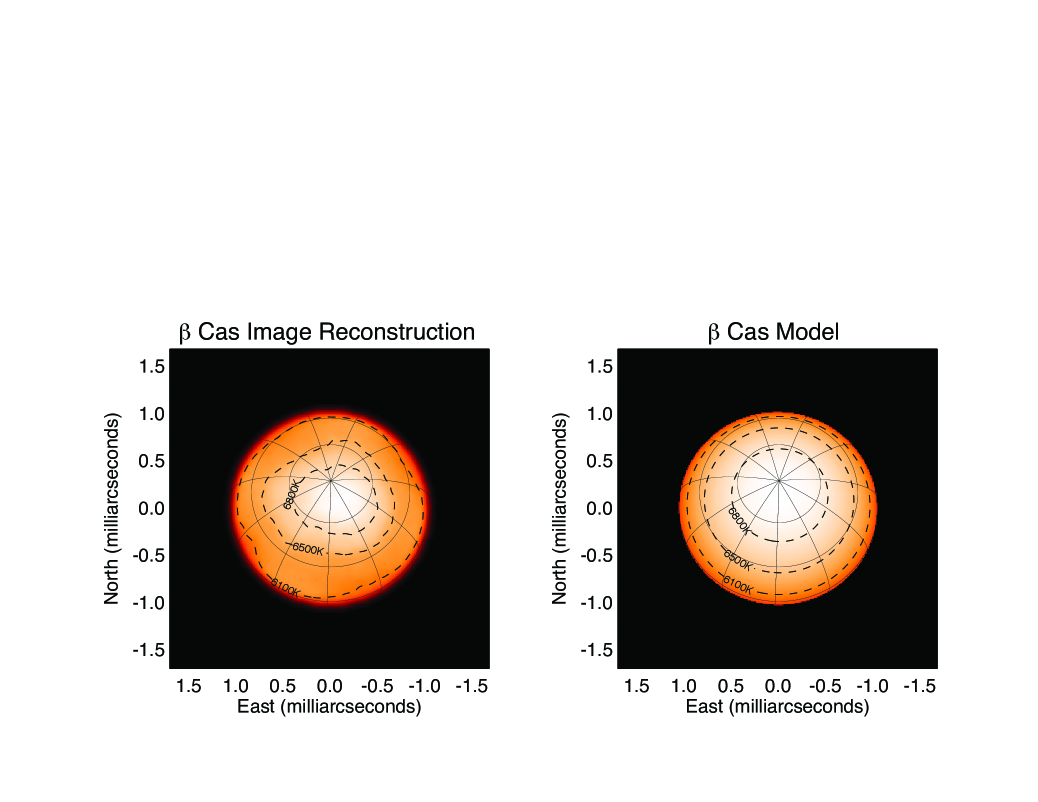
Figure 4: Images of $\beta$ Cas . The left one shows the surface intensity distribution of $\beta$ Cas from MACIM, overplotted with latitudes and longitudes from the model. The angular resolution is 0.57  mas(milli-arcsecond). The dashed contours represent the surface brightness temperatures of the image. The right one shows the image from model fitting, overplotted with brightness temperature contour from the model. The reduced $\chi^{2}$ of the images from MACIM and model fitting are 1.20 and 1.36.

The left panel of Figure 5 shows the image of $\alpha$ Leo with latitudes and longitudes from the model, and surface brightness temperature contours. The reduced $\chi^{2}$ of the image is 0.78. The right one shows the image from model fitting. As opposed to $\beta$ Cas , $\alpha$ Leo is almost equator-on and the dark equator stretches along the North-South direction. One noticeable phenomenon is that the poles are not located exactly in the hot region. This is because in this particular case the poles at the stellar image edge look cooler due to lime-darkening, causing the brightest regions to shift towards the center of the image.

…..

Figure 5: Images of $\alpha$ Leo . The notations are all the same as those in images of $\beta$ Cas (see Fig. 4). The angular resolution is 0.55  mas. The reduced $\chi^{2}$ of the images from MACIM and model fitting are 0.78 and 1.32.

5 Stellar Evolution Tracks

One interesting topic for rapidly rotating stars is to locate their positions on the Hertzsprung-Russell (HR) diagram and compare with stellar models. This topic contains two issues. First, traditional photometry observations only see the apparent luminosities $\emph{L}_{\mathrm{app}}$ and apparent effective temperatures $\emph{T}_{\mathrm{app}}^{\mathrm{eff}}$ which depend on stellar inclination angles; the bolometric luminosities $\emph{L}_{\mathrm{bol}}$ of rapid rotators are hidden from the observers. Interferometric observations allow us to construct 2-D surface models of stars, thus to obtain the $\emph{L}_{\mathrm{bol}}$ (Zhao et al., 2009). We obtain the gravity and temperature distributions across the stellar surface from the model fitting. From Kurucz model, we are able to retrieve intensities from each patch of stellar surface, and then integrate the radiation all over the star to obtain the bolometric luminosity $\emph{L}_{\mathrm{bol}}$ . By comparison we also compute an inclination curve which shows stellar $\emph{L}_{\mathrm{app}}$ and $\emph{T}_{\mathrm{app}}^{\mathrm{eff}}$ as a function of the inclination angle, and we can mark the one corresponding to its inclination from the model fitting. The $\emph{L}_{\mathrm{app}}$ can be calculated by $\emph{L}_{\mathrm{app}}$ = 4$\pi d^{2}$$\emph{F}_{\mathrm{bol}}$, where d is the distance and $\emph{F}_{\mathrm{bol}}$ is the bolometric flux computed by integrating flux from each grid over the projected area. Then the $\emph{T}_{\mathrm{app}}^{\mathrm{eff}}$ is obtained by $\sigma$($\emph{T}_{\mathrm{app}}^{\mathrm{eff}}$ )⁴ = $\pi d^{2}$$\emph{F}_{\mathrm{bol}}$/$\emph{A}_{\mathrm{proj}}$, where $\emph{A}_{\mathrm{proj}}$ is the projected area.

Second, typical HR diagrams are constructed for non-rotating stars, it is inappropriate to place a rapid rotating star on such diagrams. A rapidly rotating star shows a little lower $\emph{L}_{\mathrm{bol}}$ than $\emph{L}_{\mathrm{nr}}$ from its non-rotating equivalent (an imaginary spherical star which a rapid rotator would turn out to be if it spins down to no angular velocity), meaning a rotating star will evolve as a lower mass star on HR diagram. Therefore the interpreted mass and age from the rotating star deviates from the true values. To partially solve this problem, one has to convert the properties of a rapidly rotating star to its non-rotating equivalent. Studies have shown that the bolometric luminosity and polar radius do not change much as a star spins up. Following this, we alter the traditional HR diagram to a new one with axes of bolometric luminosity and polar radius ($\emph{L-R}_{\rm{pol}}$ diagram), and locate rotating stars on the new diagram to infer the mass and age (Peterson et al., 2006, private communication, 2010). To compare with the astronomy-friendly HR diagrams, one can also translate these two values of non-rotating equivalents into $\emph{L}_{\mathrm{nr}}$ and $\emph{T}_{\mathrm{nr}}^{\mathrm{eff}}$ .

The left panels of Fig. 6 and 7 show $\beta$ Cas and $\alpha$ Leo on $\emph{L-R}_{\rm{pol}}$ diagrams from $Y^{2}$ model (Yi et al., 2001, 2003; Demarque et al., 2004). The cross and square symbols represent the bolometric luminosity and polar radius before and after the rotational correction respectively (Sackmann, 1970). The corrections are trivial: $\emph{L}_{\mathrm{nr}}$ and R_pol,nr decrease by 5.5% and 1.3% respectively for a 2 solar mass star as it spins up to close to critical speed. So on $\emph{L-R}_{\rm{pol}}$ diagrams one may even directly use $\emph{L}_{\mathrm{bol}}$ and R_pol of a rotating star for rough interpretations of its mass and age. We have begun work on a more exact formulation using a new grid of rotating models, but this is the subject of future detailed paper.

The traditional HR diagrams are shown in the right panels of Fig. 6 and 7. The solid lines are the inclination curves, which show the $\emph{L}_{\mathrm{app}}$ and $\emph{T}_{\mathrm{app}}^{\mathrm{eff}}$ as a function of inclination angles. The star symbols on the curve represent the estimated inclination angles. The square symbols stand for $\emph{L}_{\mathrm{nr}}$ and $\emph{T}_{\mathrm{nr}}^{\mathrm{eff}}$ of the non-rotating equivalent. The position of non-rotating equivalent on HR diagram deviates severely from the position of the rapidly rotating equivalent based on its apparent values. For instance, Regulus would be about 0.08 Gyr older and 0.5  M_⊙less massive from its $\emph{L}_{\mathrm{app}}$ and $\emph{T}_{\mathrm{app}}^{\mathrm{eff}}$ than from $\emph{L}_{\mathrm{nr}}$ and $\emph{T}_{\mathrm{nr}}^{\mathrm{eff}}$ . So we strongly recommend to correct for the effects of rotation when placing a rapidly rotating star on HR diagram. Zhao et al. (2009) didn’t adopt this correction, which may lead to an additional error in determining age and mass of rapidly rotating stars.

…..

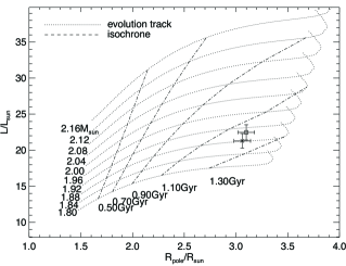
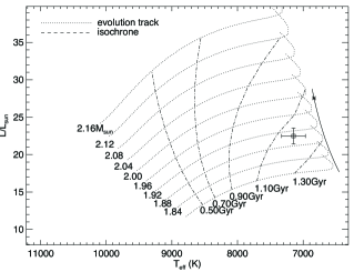
Figure 6: $\beta$ Cas positions on $\emph{L-R}_{\rm{pol}}$ (left) and Hertzsprung-Russell (right) diagrams based on $Y^{2}$ model (Yi et al., 2001, 2003; Demarque et al., 2004). In the left panel, the cross symbol with error bar stands for the rapidly rotating $\beta$ Cas based on its $\emph{L}_{\mathrm{bol}}$ and polar radius from modified von Zeipel model fitting. The square symbol with error bar is the non-rotating equivalent of $\beta$ Cas , the corrections of $\emph{L}_{\mathrm{bol}}$ and polar radius because of rotation is adopted from Sackmann (1970). In the right panel, the solid line is the inclination curve, which shows how $\emph{L}_{\mathrm{app}}$ and $\emph{T}_{\mathrm{app}}^{\mathrm{eff}}$ change as a function of inclination angles. The star symbol is $\beta$ Cas with its estimated inclination angle. The meaning of the square symbol is the same as in the left panel (see Section 5).

…..

6 Discussion

6.1 Stellar Core-Envelope Coupling

Measuring $\omega$ / $\omega_{\rm crit}$ as a function of age provides a way of studying the coupling between the stellar core and envelope in terms of angular momentum. As a star evolves along the main sequence, the core contracts and spins up due to the conservation of the angular momentum, while the spherical-shell envelope expands and spins down. $\omega_{\rm crit}$ also drops as the star expands. Given the initial rotational conditions and the evolution of stellar inner structure, the evolution of $\omega$ / $\omega_{\rm crit}$ depends only on how much the core and envelope are coupled. In the case when the core and envelope are not coupled, the angular velocity of the envelope changes roughly proportional to $\rm{R}^{-2}$. The ratio $\omega_{\rm crit}$ is proportional to $\rm{R}^{-1.5}$. So $\omega$ / $\omega_{\rm crit}$ decreases roughly as $\rm{R}^{-0.5}$ as a star expands. While in the other extreme case of solid body rotation, namely the core and envelope are fully coupled, the core transfers the most angular momentum to the envelope, and $\omega$ / $\omega_{\rm crit}$ may increase as a star expands. We can also predict its value in the past, knowing the current $\omega$ / $\omega_{\rm crit}$.

One critical component in the discussion above is the evolution model of stellar inner structure. While several such models are available for non-rotating stars, we can not find one for the general case of rotating stars. We justify that a non-rotating stellar model is a good approximation for calculating evolution of internal density profiles because rotation has very little effect on iso-potential surfaces inside the star. For instance, a rapidly rotating star with $\omega$ / $\omega_{\rm crit}$ = 0.9, its equatorial radius is elongated by only 21.6%, but gravity quickly dominates as one looks deep into the star. This means $\omega_{\rm crit}$ is much larger than angular velocity at certain radius and smaller, and the structure can again be approximately described by a non-rotating stellar model. So in the following calculation we adopt a non-rotating stellar model

By computing how the moment of inertia changes with time, we are able to calculate the evolution of $\omega$ / $\omega_{\rm crit}$for a 1.9 M_⊙ non-rotating star (Fig. 8). In the left panel, all the values are normalized to their initial values. The solid line shows the evolution of the stellar radius, the dotted and dashed lines show the evolution of the ratio $\omega$ / $\omega_{\rm crit}$ when the core and envelope are fully coupled and uncoupled. When the core and envelope are uncoupled, the ratio drops as the star expands as expected. When the core and envelope are fully coupled, the ratio actually increases a little due to the transference of angular momentum from the core to the envelope. This result may explain high $\omega$ / $\omega_{\rm crit}$ value of $\beta$ Cas .

In the right panel, we use the ratio $\omega$ / $\omega_{\rm crit}$ = 0.92 from model fitting as the current value of $\beta$ Cas , and trace back to its previous values in the extreme cases of full-coupling and no coupling. We notice that if the core and envelope are not well-coupled (dashed line), the ratio will exceed the unit in the past, which is not allowed. On the other hand if they are totally coupled (dotted line), the ratio value remains below 1. Reading off the panel, $\omega$ / $\omega_{\rm crit}$ changes more rapidly in the past $\sim$ 0.5  Gyr if the core and envelope are not coupled. These results suggest that during the stellar evolution of $\beta$ Cas , the angular momentum is efficiently transferred from the core to the envelope in the past 500 Myr. These results seem to confirm earlier findings by Danziger & Faber (1972) based on analysis of $v~{}sin~{}i$ statistics.

…..

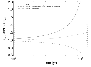
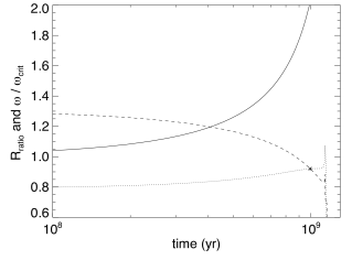
Figure 8: The evolution of stellar rotation. The model is adopted from the evolution of a 1.90  M_⊙ non-rotating star (Paxton, 2004, the web-browser interface is developed and maintained by Rich Townsend). The left panel: solid line is the ratio of the stellar radius to its value at the beginning of main sequence; dashed line is the ratio of $\omega$ / $\omega_{\rm crit}$ ($\omega$ is angular velocity; $\omega_{\rm crit}$is the critical angular velocity when the centrifugal force balances the gravity at the equator) to its initial value when the core and envelope are not coupled; dotted line is the ratio when they are totally coupled. The right panel: using the current $\omega$ / $\omega_{\rm crit}$ value (represented by asterisk) from model fitting, track back to its previous values assuming uncoupling and total coupling of the core and envelope.

6.2 Gravity Darkening Coefficient

Von Zeipel brought up the idea of gravity darkening in 1924 and predicted the standard value of $\beta$ to be 0.25 for stars with fully radiative envelope. Our group have studied five rapid rotators ($\alpha$ Aql, $\alpha$ Cep, $\alpha$ Oph, $\alpha$ Leo, $\beta$ Cas) up to now, four of them show non-standard Gravity darkening coefficient ($\beta$) values from the modified von Zeipel model fitting. $\alpha$ Oph was only fitted with $\beta$-fixed model because of the high degeneracy between gravity darkening coefficient and rotational speed due to its almost equator-on orientation (Zhao et al., 2009).

In Fig. 9 we plot the results of $\beta$ versus temperature for the four targets with their gravity darkening coefficients obtained from the modified von Zeipel model fitting. The shadow areas show the temperature ranges from the pole to equator and the 1-$\sigma$ uncertainties of $\beta$ from the model fitting for each star. For comparison, we also plot the solid line representing the predicted relation between $\beta$ and temperature adopted from Claret (2000). We digitize the evolution plot of a 2 solar mass star in Claret (2000) paper and extend $\beta$ to high temperature 14500 K with $\beta$ fixed to 0.25. We should point out that the predicted relation shifts a little to lower temperature for stars with higher masses, but it is not a big issue in our case. For $\alpha$ Cep, $\alpha$ Aql and $\beta$ Cas, their masses are close to 2  M_⊙, so they can share the same relation. $\alpha$ Leo is much more massive than 2  M_⊙, the predicted curve shifts to low temperature a little (less than 1000K).

…..

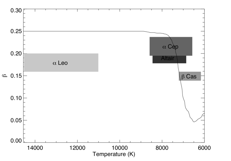
Figure 9: Gravity darkening coefficient ($\beta$) vs. temperature for four targets our group has studied. The solid line represents the theoretical relation between the gravity darkening coefficient $\beta$ and effective temperature, adopted from the evolution of a non-rotating 2 solar mass star (Claret, 2000). The curve is extended to higher temperature for comparison with $\alpha$ Leo (see section 6.2 for details). The temperature range of each star contains temperature from the poles to equator. The $\beta$ range indicates the uncertainty from the model fitting.

Fig. 9 shows that $\alpha$ Cep, $\alpha$ Aql and $\beta$ Cas partially intercept the transition area of the predicted curve, meaning that the equatorial regions might star to show convection. In our model fitting, we use a single $\beta$ to describe the relation between the gravity and temperature, instead of letting $\beta$ change as a function of temperature. This may partially explain why these three stars have non-standard $\beta$ values, because their poles could be radiation-dominated while the equators convection-dominated, the resulting $\beta$ may be some weighted values across the stellar surfaces. However the analysis here is non-physical, a detailed stellar model that includes radiation and convection in a rapidly rotating star is required to fully understand the gravity darkening law of these stars with intermediate temperatures.

However $\alpha$ Leo has such high temperature range that even the equator is supposed to be fully radiative theoretically. So the poles and equator will share the same $\beta$ = 0.25, justifying the standard von Zeipel model in this case. But our result still prefers non-standard $\beta$ = $0.188^{+0.012}_{-0.029}$ . One possible explanation is that even at such high temperature, the envelope is not fully radiative. Tassoul (2000) concludes that solid-body rotation is impossible for a pseudo-barotrope in static radiative equilibrium. The solid-body rotation will disrupt the constancy of the temperature and pressure over the stellar surface, and cause the temperature and pressure gradients between the equator and poles. The gradients will induce a flow of matter which forms a permanent meridional circulation and break down the strict radiative equilibrium. The matter flow may further lead to the failure of our model assumption: solid-body rotation. The material from higher latitudes carries less angular momentum than those from lower latitudes. The meridional flows moving towards higher or lower latitudes will speed up or slow down the rotational speed of local material on their way, which triggers differential rotation.

Another study from Lovekin et al. (2006) compares the effective temperature distribution across the surface of a 6.5  M_⊙ solid-body rotator between a stellar evolution model with rotation (ROTORC) and von Zeipel’s law, and finds that the temperature distribution is shallower in the model which is consistent with lower $\beta$ value we obtained from $\alpha$ Leo . A few observations on W UMa systems (Kitamura & Nakamura, 1988; Pantazis & Niarchos, 1998) roughly confirm von Zeipel’s law, but with very large scatter. The material flows on the surfaces of these stars are less complicated due to an important feature of the binary systems: the stars are tidally locked by their companions. Hence the stellar differential rotations are effectively depressed and the resulting solid-body rotations are well regulated. Therefore these stars may maintain radiation-dominated envelopes which validate the standard von Zeipel model.

Based on the similar $\beta$ value found for all our objects and for $\alpha$ Leo in particular, we recommend researchers adopt a new standard $\beta$=0.19 for future modeling of rapid rotating stars with radiative envelopes.

7 Conclusion

We have studied two rapid rotators with extreme spectral type: $\beta$ Cas and $\alpha$ Leo observed by CHARA-MIRC. By fitting the modified von Zeipel model, namely the solid-body rotation model with free-$\beta$ gravity darkening law, to observed infrared interferometry data and V and H photometric fluxes, we find both stars are rotating at close to critical speed: $\omega$ / $\omega_{\rm crit}$= 0.92 and 0.96. The fast rotations elongate their equators by 24% and 30% compared with their poles, and their equatorial temperatures are 1000K and 3000K cooler than their polar values. We estimated the mass of $\alpha$ Leo to be 4.15 $\pm$ 0.06  M_⊙ from both $\emph{L-R}_{\rm{pol}}$ and HR diagrams corrected for rotational effect, and it is much higher than 3.4 $\pm$ 0.2  M_⊙found by McAlister et al. (2005). We have also reconstructed aperture synthesis images using MACIM. The images are consistent with the temperature distribution from the model fitting.

We discussed the evolution of $\omega$ / $\omega_{\rm crit}$. The ratio could increase or decrease depending on how much stellar cores and envelopes are coupled. In the case of fully coupling, $\omega$ / $\omega_{\rm crit}$ increases a little during main sequence and sub-giant branch due to the angular momentum transferred from the core to the envelope. Our study on $\beta$ Cas, which is about 1.18  Gyrold but still rotating at 92% of its critical speed, suggests the core and envelope are well coupled during the evolution.

All our targets from the modified von Zeipel model fitting prefer the non-standard gravity darkening coefficients, especially in the case of $\alpha$ Leo whose envelope should be fully radiative because of the high surface temperature range 11010K - 14520K. One possible reason is that solid-body rotation breaks down the constancy of temperature and pressure on the stellar surface and induces meridional flow, which violates strict radiative equilibrium. Furthermore the meridional flow may result in differential rotation which causes the failure of our solid-body rotation assumption. To explore this possibility in the future, we will construct a differential rotation model to fit observed high resolution spectra of these rapidly rotating stars. Until better models are created, we recommend using the empirically-determined gravity-darkening coefficient $\beta$ = 0.19 for rapidly-rotating stars with radiative envelopes.

Appendix A Appendix

Visibility data and fitting results from one single night are shown in Fig. 10 and 11. The upper left panels show all 7 and 5 nights combined visibility data of $\beta$ Cas and $\alpha$ Leo respectively, overplotted with the visibility curves of uniform disks with diameters of major and minor axises from model fitting. The other panels show the model fitting and imaging results compared with one single night data. The date of that night of $\beta$ Cas is Oct. 22nd 2009, and that of $\alpha$ Leo is Dec 8th 2008.

…..

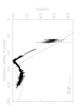
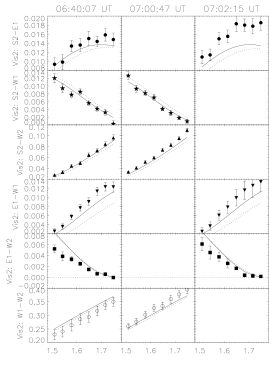
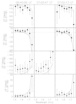
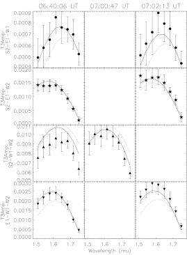
Figure 10: Upper left panel: all seven nights visibility data of $\beta$ Cas . The solid line and dotted line show the visibility curves of uniform disks with diameters of major and minor axis of $\beta$ Cas from model fitting. The rest panels: the modified von Zeipel model (solid line) and MACIM image (dotted line, see section 4) vs. observed data (filled points with error bars) of $\beta$ Cas from one single night. The reduced $\chi^{2}$ of model is 1.36 and that of image is 1.20. The eight data points in each sub-panel are from eight sub-channels of MIRC observation across H band. The x axis shows the wavelengths corresponding to the data points. The y axis shows which telescopes of CHARA have been used.

…..

References

- Abt et al. (2002) Abt, H. A., Levato, H., & Grosso, M. 2002, ApJ, 573, 359
- Abt & Morrell (1995) Abt, H. A. & Morrell, N. I. 1995, ApJS, 99, 135
- Aufdenberg et al. (2006) Aufdenberg, J. P., Mérand, A., Coudé du Foresto, V., Absil, O., Di Folco, E., Kervella, P., Ridgway, S. T., Berger, D. H., ten Brummelaar, T. A., McAlister, H. A., Sturmann, J., Sturmann, L., & Turner, N. H. 2006, ApJ, 645, 664
- Barnes et al. (1978) Barnes, T. G., Evans, D. S., & Moffett, T. J. 1978, MNRAS, 183, 285
- Bernacca & Perinotto (1970) Bernacca, P. L. & Perinotto, M. 1970, Contributions dell’Osservatorio Astrofisica dell’Universita di Padova in Asiago, 239, 1
- Bonneau et al. (2006) Bonneau, D., Clausse, J., Delfosse, X., Mourard, D., Cetre, S., Chelli, A., Cruzalèbes, P., Duvert, G., & Zins, G. 2006, A&A, 456, 789
- Che et al. (2010) Che, X., Monnier, J. D., & Webster, S. 2010, in Presented at the Society of Photo-Optical Instrumentation Engineers (SPIE) Conference, Vol. 7734, 91
- Claret (1998) Claret, A. 1998, A&AS, 131, 395
- Claret (2000) —. 2000, A&A, 359, 289
- Cutri et al. (2003) Cutri, R. M., Skrutskie, M. F., van Dyk, S., Beichman, C. A., Carpenter, J. M., Chester, T., Cambresy, L., Evans, T., Fowler, J., Gizis, J., Howard, E., Huchra, J., Jarrett, T., Kopan, E. L., Kirkpatrick, J. D., Light, R. M., Marsh, K. A., McCallon, H., Schneider, S., Stiening, R., Sykes, M., Weinberg, M., Wheaton, W. A., Wheelock, S., & Zacarias, N. 2003, 2MASS All Sky Catalog of point sources.
- Danziger & Faber (1972) Danziger, I. J. & Faber, S. M. 1972, A&A, 18, 428
- Daszyńska & Cugier (2003) Daszyńska, J. & Cugier, H. 2003, Advances in Space Research, 31, 381
- Demarque et al. (2004) Demarque, P., Woo, J., Kim, Y., & Yi, S. K. 2004, ApJS, 155, 667
- Domiciano de Souza et al. (2003) Domiciano de Souza, A., Kervella, P., Jankov, S., Abe, L., Vakili, F., di Folco, E., & Paresce, F. 2003, A&A, 407, L47
- Ducati (2002) Ducati, J. R. 2002, VizieR Online Data Catalog, 2237, 0
- Gies et al. (2008) Gies, D. R., Dieterich, S., Richardson, N. D., Riedel, A. R., Team, B. L., McAlister, H. A., Bagnuolo, Jr., W. G., Grundstrom, E. D., Štefl, S., Rivinius, T., & Baade, D. 2008, ApJ, 682, L117
- Glebocki & Stawikowski (2000) Glebocki, R. & Stawikowski, A. 2000, Acta Astron., 50, 509
- Gray et al. (2003) Gray, R. O., Corbally, C. J., Garrison, R. F., McFadden, M. T., & Robinson, P. E. 2003, AJ, 126, 2048
- Gray et al. (2001) Gray, R. O., Graham, P. W., & Hoyt, S. R. 2001, AJ, 121, 2159
- Holmberg et al. (2007) Holmberg, J., Nordström, B., & Andersen, J. 2007, A&A, 475, 519
- Ireland et al. (2006) Ireland, M. J., Monnier, J. D., & Thureau, N. 2006, in Presented at the Society of Photo-Optical Instrumentation Engineers (SPIE) Conference, Vol. 6268, 58
- Johnson & Morgan (1953) Johnson, H. L. & Morgan, W. W. 1953, ApJ, 117, 313
- Kervella & Fouqué (2008) Kervella, P. & Fouqué, P. 2008, A&A, 491, 855
- Kharchenko et al. (2009) Kharchenko, N. V., Piskunov, A. E., Röser, S., Schilbach, E., Scholz, R., & Zinnecker, H. 2009, A&A, 504, 681
- Kitamura & Nakamura (1988) Kitamura, M. & Nakamura, Y. 1988, Ap&SS, 145, 117
- Kurucz (1992) Kurucz, R. L. 1992, in IAU Symposium, Vol. 149, The Stellar Populations of Galaxies, ed. B. Barbuy & A. Renzini, 225–+
- Lovekin et al. (2006) Lovekin, C. C., Deupree, R. G., & Short, C. I. 2006, ApJ, 643, 460
- MacFadyen & Woosley (1999) MacFadyen, A. I. & Woosley, S. E. 1999, ApJ, 524, 262
- McAlister et al. (2005) McAlister, H. A., ten Brummelaar, T. A., Gies, D. R., Huang, W., Bagnuolo, Jr., W. G., Shure, M. A., Sturmann, J., Sturmann, L., Turner, N. H., Taylor, S. F., Berger, D. H., Baines, E. K., Grundstrom, E., Ogden, C., Ridgway, S. T., & van Belle, G. 2005, ApJ, 628, 439
- Mérand (2008) Mérand, A. 2008, in EAS Publications Series, Vol. 28, EAS Publications Series, ed. S. Wolf, F. Allard, & P. Stee, 53–59
- Meynet & Maeder (2000) Meynet, G. & Maeder, A. 2000, A&A, 361, 101
- Monnier et al. (2004) Monnier, J. D., Berger, J., Millan-Gabet, R., & ten Brummelaar, T. A. 2004, in Presented at the Society of Photo-Optical Instrumentation Engineers (SPIE) Conference, Vol. 5491, 1370, ed. W. A. Traub, 1370–+
- Monnier et al. (2006) Monnier, J. D., Pedretti, E., Thureau, N., Berger, J., Millan-Gabet, R., ten Brummelaar, T., McAlister, H., Sturmann, J., Sturmann, L., Muirhead, P., Tannirkulam, A., Webster, S., & Zhao, M. 2006, in Presented at the Society of Photo-Optical Instrumentation Engineers (SPIE) Conference, Vol. 6268, 55
- Monnier et al. (2007) Monnier, J. D., Zhao, M., Pedretti, E., Thureau, N., Ireland, M., Muirhead, P., Berger, J., Millan-Gabet, R., Van Belle, G., ten Brummelaar, T., McAlister, H., Ridgway, S., Turner, N., Sturmann, L., Sturmann, J., & Berger, D. 2007, Science, 317, 342
- Monnier et al. (2008) Monnier, J. D., Zhao, M., Pedretti, E., Thureau, N., Ireland, M., Muirhead, P., Berger, J., Millan-Gabet, R., Van Belle, G., ten Brummelaar, T., McAlister, H., Ridgway, S., Turner, N., Sturmann, L., Sturmann, J., Berger, D., Tannirkulam, A., & Blum, J. 2008, in Presented at the Society of Photo-Optical Instrumentation Engineers (SPIE) Conference, Vol. 7013, 1
- Morel & Magnenat (1978) Morel, M. & Magnenat, P. 1978, A&AS, 34, 477
- Pantazis & Niarchos (1998) Pantazis, G. & Niarchos, P. G. 1998, A&A, 335, 199
- Paxton (2004) Paxton, B. 2004, PASP, 116, 699
- Pedretti et al. (2009) Pedretti, E., Monnier, J. D., Brummelaar, T. T., & Thureau, N. D. 2009, New A Rev., 53, 353
- Peterson et al. (2006) Peterson, D. M., Hummel, C. A., Pauls, T. A., Armstrong, J. T., Benson, J. A., Gilbreath, G. C., Hindsley, R. B., Hutter, D. J., Johnston, K. J., Mozurkewich, D., & Schmitt, H. R. 2006, Nature, 440, 896
- Rachford & Foight (2009) Rachford, B. L. & Foight, D. R. 2009, ApJ, 698, 786
- Reiners (2006) Reiners, A. 2006, A&A, 446, 267
- Rhee et al. (2007) Rhee, J. H., Song, I., Zuckerman, B., & McElwain, M. 2007, ApJ, 660, 1556
- Richichi & Percheron (2002) Richichi, A. & Percheron, I. 2002, A&A, 386, 492
- Sackmann (1970) Sackmann, I. J. 1970, A&A, 8, 76
- Schröder et al. (2009) Schröder, C., Reiners, A., & Schmitt, J. H. M. M. 2009, A&A, 493, 1099
- Slettebak (1963) Slettebak, A. 1963, AJ, 68, 292
- Stoeckley et al. (1984) Stoeckley, T. R., Carroll, R. W., & Miller, R. D. 1984, MNRAS, 208, 459
- Tassoul (2000) Tassoul, J. 2000, Stellar Rotation, ed. Tassoul, J.-L.
- van Belle et al. (2006) van Belle, G. T., Ciardi, D. R., ten Brummelaar, T., McAlister, H. A., Ridgway, S. T., Berger, D. H., Goldfinger, P. J., Sturmann, J., Sturmann, L., Turner, N., Boden, A. F., Thompson, R. R., & Coyne, J. 2006, ApJ, 637, 494
- van Belle et al. (2001) van Belle, G. T., Ciardi, D. R., Thompson, R. R., Akeson, R. L., & Lada, E. A. 2001, ApJ, 559, 1155
- van Leeuwen (2007) van Leeuwen, F. 2007, A&A, 474, 653
- von Zeipel (1924a) von Zeipel, H. 1924a, MNRAS, 84, 665
- von Zeipel (1924b) —. 1924b, MNRAS, 84, 684
- Yi et al. (2001) Yi, S., Demarque, P., Kim, Y., Lee, Y., Ree, C. H., Lejeune, T., & Barnes, S. 2001, ApJS, 136, 417
- Yi et al. (2003) Yi, S. K., Kim, Y., & Demarque, P. 2003, ApJS, 144, 259
- Zhao et al. (2009) Zhao, M., Monnier, J. D., Pedretti, E., Thureau, N., Mérand, A., ten Brummelaar, T., McAlister, H., Ridgway, S. T., Turner, N., Sturmann, J., Sturmann, L., Goldfinger, P. J., & Farrington, C. 2009, ApJ, 701, 209