Extracting the photoproduction cross section off the neutron $\gamma n\!\to\!\pi^{-}p\,$ from deuteron data with FSI effects

Abstract

The incoherent pion photoproduction reaction $\gamma d\!\to\!\pi^{-}pp$ is considered theoretically in a wide energy region $E_{th}\leq E_{\gamma}\leq 2700$ MeV. The model applied contains the impulse approximation as well as the NN- and $\pi N$-FSI amplitudes. The aim of the paper is to study a reliable way for getting the information on elementary $\gamma n\!\to\!\pi^{-}p$ reaction cross section beyond the impulse approximation for $\gamma d\!\to\!\pi^{-}pp$. For the elementary $\gamma N\!\to\!\pi N$, $N\!N\!\to\!N\!N$, and $\pi N\!\to\!\pi N$ amplitudes, the results of the GW DAC are used. There are no additional theoretical constraints. The calculated cross sections $d\sigma\!/d\Omega(\gamma d\!\to\!\pi^{-}pp)$ are compared with existing data. The procedure used to extract information on the differential cross section $d\sigma\!/d\Omega(\gamma n\!\to\!\pi^{-}p)$ on the neutron from the deuteron data using the FSI correction factor $R$ is discussed. The calculations for $R$ versus $\pi^{-}p$ CM angle $\theta_{1}$ of the outgoing pion are performed at different photon-beam energies with kinematical cuts for “quasi-free” process $\gamma n\!\to\!\pi^{-}p$. The results show a sizeable FSI effect $R\neq 1$ from $S$-wave part of $pp$-FSI at small angles close to $\theta_{1}\sim 0$: this region narrows as the photon energy increases. At larger angles, the effect is small ($|R\!-\!1|\ll 1$) and agrees with estimations of FSI in the Glauber approach.

I Introduction

The $N^{\ast}$ family of nucleon resonances has many well-established members PDG , several of which exhibit overlapping resonances with very similar masses and widths, but with different $J^{P}$ spin-parity values. Apart from the $N(1535)1/2^{-}$ state, the known proton and neutron photo-decay amplitudes have been determined from analyses of single-pion photoproduction. The present work studies the region from threshold to the upper limit of the SAID analyses, which is $W=2.5$ GeV. There are two closely spaced states above the $\Delta(1232)3/2^{+}$: $N(1520)3/2^{-}$ and $N(1535)1/2^{-}$. Up to a CM energy of $W\approx 1800$ MeV, this region also encompasses a sequence of six overlapping states: $N(1650)1/2^{-}$, $N(1675)5/2^{-}$, $N(1680)5/2^{+}$, $N(1700)3/2^{-}$, $N(1710)1/2^{+}$, and $N(1720)3/2^{+}$.

One critical issue in the study of meson photoproduction on the nucleon comes from isospin. While isospin can change at the photon vertex, it must be conserved at the final hadronic vertex. Only with good data on both proton and neutron targets can one hope to disentangle the isoscalar and isovector electromagnetic couplings of the various N^∗ and $\Delta^{\ast}$ resonances (see, Refs. Wat ; Walker ), as well as the isospin properties of the non-resonant background amplitudes. The lack of $\gamma n\to\pi^{-}p$ and $\pi^{0}n$ data does not allow us to be as confident about the determination of neutron couplings relative to those of the proton. Some of the $N^{\ast}$ baryons ($N(1675)5/2^{-}$, for instance) have stronger electromagnetic couplings to the neutron relative to the proton, but the parameters are very uncertain PDG . Data on the $\gamma N\!\to\!\pi N$ reactions are needed to improve the amplitudes and expand them to higher energies.

Incoherent pion photoproduction on the deuteron is interesting in various aspects of nuclear physics, and particularly provides information on the elementary reaction on the neutron, i.e., $\gamma n\!\to\!\pi N$. Final-state-interaction (FSI) plays a critical role in the state-of-the-art analysis of the $\gamma N\!\to\!\pi N$ interaction as extracted from $\gamma d\!\to\!\pi NN$ data. The FSI was first considered in Refs. Migdal ; Watson as responsible for the near threshold enhancement (Migdal-Watson effect) in the $NN$-mass spectrum of the meson production reaction $NN\to NNx$. In Ref. Baru , the FSI amplitude was studied in detail. Calculations of $NN$- and $\pi N$-FSI for the reactions $\gamma d\!\to\!\pi NN$ can be traced back to Refs. BL ; La78 ; La81 . In Refs. La78 ; La81 , the elementary $\gamma N\!\to\!\pi N$ amplitude, constructed in Ref. BL from the Born terms and $\Delta(1232)3/2^{+}$ contribution, was used in $\gamma d\!\to\!\pi NN$ calculations with FSI terms taken into account. Good descriptions of the available deuteron data for charged pion photoproduction in the threshold and $\Delta(1232)3/2^{+}$ regions were obtained.

Further developments of this topic (see Dar ; DAS ; Fix ; Lev06 ; Schwamb ; Lev10 ; Dar1 ; La06 and references therein) included improvements of the elementary $\gamma N\!\to\!\pi N$ amplitude, predictions for the unpolarized and polarized (polarized beam, target or both, see Dar ; Fix ; Lev06 ; Schwamb ; Lev10 ; Dar1 and references therein) observables in the $\gamma d\!\to\!\pi NN$ reactions, and comparison with new data. Different models for $\gamma N\!\to\!\pi N$ amplitude were used in the above mentioned papers, i.e., MAID MAID98 (Refs. Fix ; Lev06 ), SAID SAID02 (Refs. Lev06 ; Lev10 ), and MAID MAID07 (Ref. Lev10 ). As discussed in Refs. Lev06 ; Lev10 , the main uncertainties of $\gamma d\!\to\!\pi NN$ calculations stem from the model dependence of the $\gamma N\!\to\!\pi N$ amplitude. In the latest SAID SAID02 and MAID MAID07 analyses, the models for $\gamma N\!\to\!\pi N$ amplitudes are developed for the photon energies $E_{\gamma}<2.7$ GeV SAID02 and $E_{\gamma}<1.65$ GeV MAID07 , respectively. Summary results from the existing $\gamma d\!\to\!\pi NN$ calculations show that FSI effects significantly reduce the differential cross section for $\pi^{0}pn$ channel, mainly due to the $pn$ rescattering, and contribute much less in the charged-pion case, i.e., in $\pi^{+}nn$ and $\pi^{-}pp$ channels.

The role of FSI depends on the kinematical region considered. In Ref. KDT , a narrow enhancement in the $pp$-mass spectrum observed in the reaction $pp\!\to\!pp\pi^{-}$ with backward outgoing $\pi^{-}$ was explained by the $pp$-FSI. The result was shown to be model-independent, determined only by $pp$-scattering parameters for the $pp$ pair produced at high momentum transfer. In the same approach, it was shown DKT that the observed energy behavior of the total cross section of the reaction $pp\!\to\!pp\eta$ in the near threshold region can be also explained by $pp$-FSI. In Ref. La06 , the meson photoproducton on deuteron was considered at high energies ($E_{\gamma}\sim$ several GeV) and high momentum transferred to final meson. This work was focused mainly on special kinematical regions close to the logarithmic singularities of the triangle NN- and $\pi$N-FSI amplitudes, the latter are strongly enhanced. These configurations where the FSI amplitudes dominates may be interesting, say, in connection with color transparency hypothesis CT . On the other hand, to extract the neutron data, we are interested in the opposite case, i.e., when FSI is suppressed.

In this paper, the role of FSI in the $\gamma d\!\to\!\pi^{-}pp$ reaction is under consideration. Our analysis addresses the data Wei ; CLAS that come from the $\gamma d\!\to\!\pi^{-}pp$ experiment at JLab using CLAS for a wide range of photon-beam energies up to about 3.5 GeV. The calculated FSI corrections for this reaction are further used to extract the $\gamma n\!\to\!\pi^{-}p$ data that constrain the $\gamma N\to\pi N$ amplitude used in PWA and coupled channel technologies.

In our approach, the $\gamma d\!\to\!\pi^{-}pp$ amplitude has three leading terms, represented by the diagrams in Fig. 1: impulse approximation (IA) [Fig. 1(a)], $pp$-FSI [Fig. 1(b)], and $\pi$N-FSI [Fig. 1(c)] contributions. IA and $\pi$N diagrams [Figs. 1(a),(c)] include also the cross-terms between outgoing protons. It is convenient to study the FSI effects in terms of the ratio

$$R_{FSI}=(d\sigma/d\Omega_{\pi p})/(d\sigma^{IA}/d\Omega_{\pi p}),$$ (1)

i.e., the ratio of the differential cross sections $d\sigma\!/d\Omega_{\pi p}$ including the full calculations of diagrams [Figs. 1(a)–(c)] to the ($d\sigma^{IA}/d\Omega_{\pi p}$), associated with IA diagram [Fig. 1(a)], where $\Omega_{\pi p}$ is the solid angle of the relative motion in the final $\pi p$ system. The ratio $R_{FSI}$ (1) depends on different kinematical variables. It can be used to extract the differential cross sections $d\sigma\!/d\Omega$ for the reaction $\gamma n\!\to\!\pi^{-}p$ from the $\gamma d\!\to\!\pi^{-}pp$ data. We use the recent GW pion photoproduction multipoles to constrain the amplitude for the impulse approximation pr_PWA with no additional theoretical input. While for the $pp$-FSI and $\pi$N-FSI, we include the GW $N\!N$ NN_PWA and GW $\pi$N amplitudes piN_PWA , respectively, for the deuteron description, we use the wave function of the CD-Bonn potential BonnCD with S- and D-wave components included.

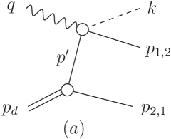
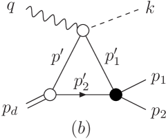
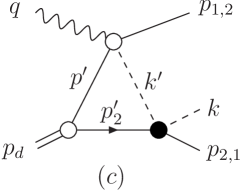
Figure 1: Feynman diagrams for the leading components of the $\gamma d\to\pi^{-}pp$ amplitude. (a) Impulse approximation, (b) $pp$-FSI, and (c) $\pi$N-FSI. Filled black circles show FSI vertices. Wavy, dashed, solid, and double lines correspond to the photons, pions, nucleons, and deuterons, respectively.

This paper is organized as follows. In Section II, we describe the model. In Subsections II.1 and II.2, we introduce the notations and write out the impulse approximation terms of the $\gamma d\!\to\!\pi NN$ amplitude. In Subsections II.3 and II.4, we derive the $N\!N$-FSI and $\pi\!N$-FSI terms of the reaction amplitude, respectively.

The results are presented in Section  III. In Subsection III.1, we compare our numerical results for the cross section $d\sigma\!/d\Omega(\gamma d\!\to\!\pi^{-}pp)$ with the DESY data and discuss the contributions from different amplitudes. In Subsection III.2, we discuss the procedure to extract the cross section $d\sigma\!/d\Omega(\gamma n\!\to\!\pi^{-}p)$ for the neutron from the $\gamma d\!\to\!\pi^{-}pp\,$ data and define the correction factor $R$. In Subsection III.3, we present the numerical results for the factor $R$ and discuss the role of the $S$-wave $pp$-FSI. In Subsection III.4, we estimate the $R$ factor in the Glauber approach. The conclusion is given in Section IV.

II Model for $\gamma d\to\pi^{-}pp$ amplitude

II.1 Kinematical notations

Hereafter $m$, $\mu$, and $m_{d}$ are the proton, pion, and deuteron masses, respectively; $q=\!(E_{\gamma},\mbox{\boldmath$q$})$, $p_{d}=\!(E_{d},\mbox{\boldmath$p$}_{d})$, $k=\!(\omega,\mbox{\boldmath$k$})$, and $p_{i}=\!(E_{i},\mbox{\boldmath$p$}_{i})$ ($i\!=\!1,2$) are the 4-momenta of the initial photon, deuteron and final pion, nucleons, respectively; $k^{\prime}=\!(\omega^{\prime},\mbox{\boldmath$k$}^{\prime})$, $p^{\prime}=\!(E^{\prime},\mbox{\boldmath$p$}^{\prime})$, and $p^{\prime}_{i}=\!(E^{\prime}_{i},\mbox{\boldmath$p$}^{\prime}_{i})$ are the 4-momenta of the intermediate particles. The 4-momenta are shown in Fig. 1. The total energies $E_{\gamma},\,E_{d},\,\cdots\,E^{\prime}_{i}$ and 3-momenta $\mbox{\boldmath$q$},\,\mbox{\boldmath$p$}_{d},\,\cdots\,\mbox{\boldmath$p$}^{\prime}_{i}$ are given in the laboratory system (LS), i.e., in the deuteron rest frame, where $\mbox{\boldmath$p$}_{d}=0$ and $E_{d}=m_{d}$.

The cross-section element $d\sigma(\gamma d\!\to\!\pi^{-}pp)$, according to the usual conventions for invariant amplitudes and phase spaces (see Appendix V.1), can be written in the form

$$d\sigma=\frac{1}{2}\,\frac{\overline{|M_{\gamma d}|^{2}}}{4E_{\gamma}m_{d}}\,d\tau_{3},~{}~{}~{}d\tau_{3}=\frac{d\,^{3}p_{2}}{(2\pi)^{3}\,2E_{2}}\,d\tau_{2},~{}~{}~{}d\tau_{2}=\frac{k_{1}d\Omega_{1}}{(4\pi)^{2}\ W_{1}}.$$ (2)

Here: $M_{\gamma d}$ is the $\gamma d\!\to\!\pi^{-}pp$ invariant amplitude; $\overline{|M_{\gamma d}|^{2}}$ is the square $|M_{\gamma d}|^{2}$, calculated for unpolarized particles; $d\tau_{3}$ is the $\pi NN$ phase space element, written in terms of the $\pi p_{1}$-pair phase space element $d\tau_{2}$ and 3-momentum $\mbox{\boldmath$p$}_{2}$ of the 2nd proton; the factor $\frac{1}{2}$ in $d\sigma$ (2) takes into account that the final protons are identical; $k_{1}$ and $\Omega_{1}$ are the relative momentum and solid angle of relative motion in the $\pi p_{1}$ system, respectively; $W_{1}$ is the effective mass of the $\pi p_{1}$ system.

II.2 Impulse-approximation amplitudes

Let us use the formalism of Ref. Tar , which is similar to that of Gross Gross in the case of small nucleon momenta $|\mbox{\boldmath$p$}|^{2}/m\ll m$ in the deuteron vertex. Then, the impulse-approximation term $M_{a}$ [Fig. 1(a)] of the $\gamma d\!\to\!\pi NN$ amplitude can be written in the form

$$M_{a}=M^{(1)}_{a}+M^{(2)}_{a},$$ (3)

$$M^{(1)}_{a}=\bar{u}_{1}\,\hat{M}_{\gamma N}^{(1)}\,i\hat{G}_{N}(p\,^{\prime})\,i\hat{\Gamma}_{d}(p_{2}\!-\!p\,^{\prime})\,u^{c}_{2},~{}~{}~{}~{}~{}M^{(2)}_{a}=-M^{(1)}_{a}(N_{1}\!\leftrightarrow\!N_{2}).$$

Here: $u_{i}$ is the bispinor (isospinor also) of the $i$-th final nucleon, $\bar{u}u=2m$; $u^{c}=\tau_{2}U_{c}\bar{u}^{T}=\tau_{2}\gamma_{2}u^{*}$, where $U_{c}=\gamma_{2}\gamma_{0}$ is the charge-conjugation matrix; $M_{\gamma N}^{(1,2)}=\bar{u}_{1,2}\hat{M}_{\gamma N}^{(1,2)}u$ is the amplitude of subprocess $\gamma N\!\to\!\pi N_{1,2}$, and $u$ is the bispinor (isospinor also) of the intermediate nucleon with 4-momentum $\,p\,^{\prime}\!=\!p_{d}-\!p_{\,2,1}$;  $\hat{G}_{N}(p\,^{\prime})=(p\!\!\!/^{\,\prime}\!+m)/(p\,^{\prime\,2}\!-m^{2}\!+i0)$ is the nucleon propagator, where $p\!\!\!/\equiv p_{\mu}\gamma_{\mu}$; $~{}\hat{\Gamma}_{d}(p_{\,2,1}-\!p\,^{\prime})$ is the $dNN$-vertex related to the deuteron wave function (DWF) as given in Appendix V.2. The amplitude $M_{a}$ is antisymmetric with respect to the nucleon permutations in accordance with the Pauli principle.

Further, we retain only the positive-energy part of the nucleon propagator $G_{N}(p\,^{\prime})$ and apply the connection between $\hat{\Gamma}_{d}$ and DWF $\hat{\Psi}_{d}$. Then, for a given spin and isospin states of the particles, we obtain

$$M^{(1)}_{a}=2\sqrt{m}\,\sum_{m^{\prime},\tau^{\prime}}\langle\pi,m_{1},\tau_{1}|\,\hat{M}_{\gamma N}^{(1)}|\,\lambda,m^{\prime},\tau^{\prime}\rangle\langle m^{\prime},\tau^{\prime},m_{2},\tau_{2}|\,\hat{\Psi}_{d}(\mbox{\boldmath$p$}_{2})|\,m_{d}\rangle,$$ (4)

and the 2nd term is $M^{(2)}_{a}=-M^{(1)}_{a}$ (with permutation of the variables of the final nucleons). Here: $m_{1,2}$, $m^{\prime}$, $\lambda$, and $m_{d}$ are spin states of the final nucleons, virtual nucleon, photon, and deuteron, respectively; $\pi$, $\tau_{1,2}$, and $\tau^{\prime}$ are isospin states of pion, final nucleons, and virtual nucleon, respectively. Substituting isospin states for the reaction $\gamma d\!\to\!\pi^{-}pp$, one gets

$$M_{a}=2\sqrt{m}~{}\sum_{m^{\prime}}~{}\bigl{[}\,\langle m_{1}|\,\hat{M}_{\gamma n}^{(1)}|\,\lambda,m^{\prime}\rangle\langle m^{\prime},m_{2}|\,\hat{\Psi}_{d}(\mbox{\boldmath$p$}_{2})|\,m_{d}\rangle$$ (5)

$$~{}~{}~{}~{}~{}~{}~{}~{}~{}~{}~{}~{}~{}~{}~{}~{}~{}~{}~{}~{}~{}~{}~{}-\langle m_{2}|\,\hat{M}_{\gamma n}^{(2)}|\,\lambda,m^{\prime}\rangle\langle m^{\prime},m_{1}|\,\hat{\Psi}_{d}(\mbox{\boldmath$p$}_{1})|\,m_{d}\rangle\,\bigr{]},$$

where now $M_{\gamma n}^{(i)}=\langle m_{i}|\,\hat{M}_{\gamma n}^{(i)}|\,\lambda,m^{\prime}\rangle$ are the $\gamma n\!\to\!\pi^{-}p_{\,i}$ amplitudes. The expressions for DWF $\langle m_{1},m_{2}\,|\hat{\Psi}_{d}(\mbox{\boldmath$p$})|\,m_{d}\rangle$ are given in Appendix V.2. The $\gamma N\!\to\!\pi N$ amplitudes $\hat{M}_{\gamma N}$ can be expressed through the Chew-Goldberger-Low-Nambu (CGLN) amplitudes CGLN (see Appendix V.3). The CGLN amplitudes as functions of the $\pi p_{i}$ invariant masses $W_{i}$ depend on the virtual nucleon momentum $p^{\prime}$ through the relation $W^{2}_{i}=(q+p^{\prime})^{2}=(k+p_{i})^{2}$. Thus, the Fermi-motion is taken into account in the $\gamma d\!\to\!\pi^{-}pp$ amplitude $M_{a}$ (5). The matrix elements $\langle m_{1}|\,\hat{M}_{\gamma N}|\,\lambda,m^{\prime}\rangle$ are given in Appendix V.4.

II.3 NN final state interaction

The NN-FSI term $M_{b}$ [Fig. 1(b)] of the $\gamma d\!\to\!\pi NN$ amplitude can be written in the form

$$M_{b}=-i\int\!\!\frac{d^{4\!}p\,^{\prime}_{2}}{(2\pi)^{4}}\,\sum_{m^{\prime}_{1},\,m^{\prime}_{2}}\!\frac{\langle m^{\prime}_{1},m^{\prime}_{2}|\,\hat{M}_{\gamma d}^{I\!A}|\,\lambda,m_{d}\rangle\langle m_{1},m_{2}|\,\hat{M}_{NN}|\,m^{\prime}_{1},m^{\prime}_{2}\rangle}{\rule{0.0pt}{12.0pt}(p\,^{\prime\,2}_{1}-m^{2}+i0)(p\,^{\prime\,2}_{2}-m^{2}+i0)}.$$ (6)

Here: $m^{\prime}_{1}$ and $m^{\prime}_{2}$ are spin states of the intermediate nucleons; the notations for $m_{1}$, $m_{2}$, $\lambda$, and $m_{d}$ are the same as in Eqs. (4) (for short, we omit isospin indices); $\hat{M}_{\gamma d}^{I\!A}$ is the amplitude of subprocess $\gamma d\!\to\!\pi NN$ in impulse approximation

$$\langle m^{\prime}_{1},m^{\prime}_{2}|\,\hat{M}_{\gamma d}^{I\!A}|\,\lambda,m_{d}\rangle=2\sqrt{m}~{}\sum_{m^{\prime}}\,\langle m^{\prime}_{1}|\,\hat{M}_{\gamma N}|\,\lambda,m^{\prime}\rangle\langle m^{\prime},m^{\prime}_{2}|\,\hat{\Psi}_{d}(\mbox{\boldmath$p$}_{2}^{\,\prime})|\,m_{d}\rangle,$$ (7)

where $\hat{M}_{NN}$ is the $NN$-scattering amplitude. The integral over the energy in Eq. (6) can be related to the residue at the nucleon (momentum $p^{\,\prime}_{\,2}$) pole with positive energy. Let us rewrite the 3-dimensional integral $\int\!d\mbox{\boldmath$p$}^{\,\prime}_{2}$ in the $N\!N$ center-of-mass system. Then, we get  $p^{\,\prime\,2}_{1}\!-\!m^{2}\!+i0=\!2W(E\!-E^{\prime}\!+i0)$, where $W$ is the $N\!N$-system effective mass, $E=\!W/2\!=\!\sqrt{p^{\,2}_{N}\!+\!m^{2}}$, $p_{N}\!=\!|\mbox{\boldmath$p$}_{N}|$, $\,E^{\prime}\!=\!\sqrt{p^{\,\prime\,2}_{N}\!+\!m^{2}}$, $p^{\,\prime}_{N}\!=\!|\mbox{\boldmath$p$}^{\,\prime}_{N}|$, and $\,\mbox{\boldmath$p$}_{N}$($\mbox{\boldmath$p$}^{\,\prime}_{N}$) is the relative 3-momentum in the final (intermediate) $N\!N$ state. We obtain

$$M_{b}=\int\!\!\frac{d\mbox{\boldmath$p$}^{\,\prime}_{N}}{(2\pi)^{3}}\,\frac{\langle\cdots\rangle}{\rule{0.0pt}{12.0pt}4E^{\prime}\,W\,(E^{\prime}-E-i0)},$$ (8)

$$\langle\cdots\rangle=\sum_{m^{\prime}_{1},\,m^{\prime}_{2}}\langle m^{\prime}_{1},m^{\prime}_{2}|\,\hat{M}_{\gamma d}^{I\!A}|\,\lambda,m_{d}\rangle\langle m_{1},m_{2}|\,\hat{M}_{NN}|\,m^{\prime}_{1},m^{\prime}_{2}\rangle.$$

One can rewrite $M_{b}$ as

$$M_{b}=M^{on}_{b}+M^{off}_{b}=\int\!\!\frac{d\mbox{\boldmath$p$}^{\,\prime}_{N}}{(2\pi)^{3}}\,\frac{\langle\cdots\rangle}{4E^{\prime}\,W}\,\left[i\pi\delta(E^{\prime}\!-\!E)+P\,\frac{1}{E^{\prime}\!-\!E}\right].$$ (9)

Here, $M^{on}_{b}$ and $M^{off}_{b}$ are the contributions from the 1st and 2nd terms, respectively, in square brackets in the r.h.s. of Eq. (9), where $P$ means the principal part of the integral. The amplitudes $M^{on}_{b}$ and $M^{off}_{b}$ correspond to the on-shell and off-shell intermediate nucleons, respectively. For $M^{on}_{b}$, we get

$$M^{on}_{b}=i\pi\!\int\!\!\frac{d\mbox{\boldmath$p$}^{\,\prime}_{N}}{(2\pi)^{3}}\,\frac{\langle\cdots\rangle}{4E^{\prime}\,W}\,\,\delta(E^{\prime}\!-\!E)=\frac{ip_{N}}{32\pi^{2}W}\,\int\!d\Omega^{\prime}\,\langle\cdots\rangle,$$ (10)

where $d\Omega^{\prime}=dz^{\prime}d\varphi^{\prime}$ ($z^{\prime}=\cos\theta^{\prime}$) is the element of solid angle of relative motion of the intermediate nucleons. Consider the 2nd term $M^{off}_{b}$. Let us use Eqs. (35) of Appendix V.2 for $\hat{\Psi}_{d}(\mbox{\boldmath$p$}_{2}^{\,\prime})$ in Eq. (7) and represent the integrand $\langle\cdots\rangle$ in Eq. (8) as the sum of two terms, proportional to S- and D-wave components of DWF, i.e., $u(p^{\prime}_{2})$ and $w(p^{\prime}_{2})$. Then, we obtain

$$\begin{array}[]{c}\langle\cdots\rangle=A\,u(p^{\prime}_{2})+B\,w(p^{\prime}_{2})~{}~{}~{}(p^{\prime}_{2}=|\mbox{\boldmath$p$}^{\prime}_{2}|),\\ \rule{0.0pt}{22.0pt}\displaystyle A=2\sqrt{m}\!\sum_{m^{\prime},m^{\prime}_{1},m^{\prime}_{2}}\,\langle m^{\prime}_{1}|\,\hat{M}_{\gamma N}|\,\lambda,m^{\prime}\rangle\langle m^{\prime},m^{\prime}_{2}|\,\hat{S}_{u}|\,m_{d}\rangle,\langle m_{1},m_{2}|\,\hat{M}_{NN}|\,m^{\prime}_{1},m^{\prime}_{2}\rangle,\end{array}$$ (11)

and $B$ is given by the expression for $A$ after the replacement $\hat{S}_{u}\!\to\!\hat{S}_{w}$, where $\hat{S}_{u}$ and $\hat{S}_{w}$ are given in Eqs. (35) of Appendix V.2. The factors $A$ and $B$ contain $\gamma N$ and $N\!N$ amplitudes, spin structure of DWF, and depend on the momenta of the particles in Fig. 1(b). Note that the $N\!N$-FSI amplitude $M_{b}$ (8) takes into account the Fermi-motion, since the amplitudes $\hat{M}_{\gamma N}$ and $\hat{M}_{NN}$ depend on the intermediate momenta $p^{\prime}$ and $p^{\prime}_{2}$, respectively. In the integral $\int\!d\mbox{\boldmath$p$}^{\,\prime}_{N}=\int\!d\Omega^{\prime}dp^{\,\prime}_{N}p^{\,\prime\,2}_{N}$ (9), we take out of subintegral $\int\!dp^{\,\prime}_{N}$ the factors $A$ and $B$ (11) at $p^{\,\prime}_{N}=p_{N}$, i.e., we calculate $A$ and $B$ as well as the amplitudes $\hat{M}_{\gamma N}$ and $\hat{M}_{NN}$ with the on-shell intermediate nucleons. This approximation means that we neglect the off-shell dependence of the $\gamma N$ and $N\!N$ amplitudes in comparison with sharp momentum dependence of DWF. Then, we get

$$M^{off}_{b}=\oint\frac{d\mbox{\boldmath$p$}^{\,\prime}_{N}}{(2\pi)^{3}}\,\frac{\langle\cdots\rangle}{4E^{\prime}\,W\,(E^{\prime}\!-\!E)}\,=\frac{1}{32\pi^{2}W}\int\!d\Omega^{\prime}\,\bigl{(}A\,I_{u}+B\,I_{w}\bigr{)},$$ (12)

$$I_{u}=\oint\frac{dp^{\,\prime}_{N}\,p^{\,\prime\,2}_{N}}{\pi E^{\prime}}\,\frac{u(p^{\prime}_{2})}{E^{\prime}\!-\!E},~{}~{}~{}~{}~{}~{}I_{w}=\oint\frac{dp^{\,\prime}_{N}\,p^{\,\prime\,2}_{N}}{\pi E^{\prime}}\,\frac{w(p^{\prime}_{2})}{E^{\prime}\!-\!E},$$

where $\oint$ denotes the principal part of the integral. We also include the formfactor $f(p^{\,\prime}_{N})$ Lev06 to parametrize the off-shell ${{}^{1}}S_{0}$ partial amplitude of $pp$-scattering and define the integrals

$$I^{(0)}_{u}=\oint\frac{dp^{\,\prime}_{N}\,p^{\,\prime\,2}_{N}}{\pi E^{\prime}}\frac{u(p^{\prime}_{2})f(p^{\,\prime}_{N})}{E^{\prime}\!-\!E},~{}~{}~{}~{}~{}f(p^{\,\prime}_{N})=\frac{p^{\,2}_{N}+\beta^{2}}{p^{\,\prime\,2}_{N}+\beta^{2}}$$ (13)

with $\beta=1.2\,$fm^-1 Lev06 ; $I^{(0)}_{w}=I^{(0)}_{u}(u(p^{\prime}_{2})\!\to\!w(p^{\prime}_{2}))$. Let us write the terms $A$ and $B$ (11) as

$$A=A_{0}+A_{1},~{}~{}~{}B=B_{0}+B_{1},$$ (14)

where $A_{0}$ ($A_{1}$) is given by Eq. (11) when only ${{}^{1}}S_{0}$ part is saved (excluded) in the $pp$-scattering amplitude $\hat{M}_{NN}$ (for $B_{0,1}$ the substitution $\hat{S}_{u}\!\to\!\hat{S}_{w}$ in Eq. (11) is implied). Combining Eqs. (9)-(13), we obtain

$$M_{b}=\int\!\frac{d\Omega^{\prime}}{32\pi^{2}W}\,\left[ip_{N}\bigl{(}A\,u(p^{\prime}_{2})+B\,w(p^{\prime}_{2})\bigr{)}+A_{0}I^{(0)}_{u}\!+\!A_{1}I_{u}\!+\!B_{0}I^{(0)}_{w}\!+\!B_{1}I_{w}\right].$$ (15)

The integrals $I_{u}$, $I_{w}$, $I^{(0)}_{u}$, $I^{(0)}_{w}$, and $\,\int\!d\Omega^{\prime}$ (15) are carried out numerically. The $N\!N$-scattering amplitude is described in Appendix V.5.

II.4 $\pi N$ final state interaction

The $\pi N$-FSI term $M_{c}$ [Fig. 1(c)] of the $\gamma d\!\to\!\pi NN$ amplitude can be written in the form

$$M_{c}=M^{(1)}_{c}+M^{(2)}_{c},~{}~{}~{}~{}M^{(1)}_{c}=-\int\!\!\frac{d\mbox{\boldmath$k$}^{\,\prime}_{2}}{(2\pi)^{3}}\,\frac{\langle\cdots\rangle}{\rule{0.0pt}{12.0pt}2E^{\prime}\,(k^{\,\prime\,2}\!-\mu^{2}\!+i0)},$$ (16)

$$\langle\cdots\rangle=\sum_{\pi^{\prime},\tau^{\prime}_{2},m^{\prime}_{2}}\langle\pi^{\prime},\tau_{1},m_{1},\tau^{\prime}_{2},m^{\prime}_{2}|\,\hat{M}_{\gamma d}^{I\!A}|\,\lambda,m_{d}\rangle\,\langle\pi,\tau_{2},m_{2}|\,\hat{M}^{(2)}_{\pi N}|\,\pi^{\prime},\tau^{\prime}_{2},m^{\prime}_{2}\rangle,$$

where the integral over the energy is also related to the residue at the nucleon pole (momentum $p^{\,\prime}_{2}$) as in Eq. (7). Here: $m^{\prime}_{2}$ and $\tau^{\prime}_{2}$ are spin and isospin states of the intermediate nucleon with 4-momentum $p^{\,\prime}_{2}$;  $\tau^{\prime}$ is isospin states of intermediate pion; the notations $m_{1,2}$, $\tau_{1,2}$, $\pi$, $\lambda$, and $m_{d}$ are given above (see Eq. (4));  $M^{(2)}_{\pi N}=\langle\pi,\tau_{2},m_{2}|\,\hat{M}^{(2)}_{\pi N}|\,\pi^{\prime},\tau^{\prime}_{2},m^{\prime}_{2}\rangle$ is the $\pi N\!\to\!\pi N_{2}$ amplitude; $\mbox{\boldmath$k$}^{\,\prime}_{2}$ is the relative 3-momentum in the intermediate $\pi N$ system. The 2nd term $M^{(2)}_{c}=-M^{(1)}_{c}$ (with permutation of the final nucleons). Substituting isospin states for the reaction $\gamma d\!\to\!\pi^{-}pp$, and making use of Eq. (7), we get the integrand $\langle\cdots\rangle$ in Eq. (16) in the form

$$\langle\cdots\rangle=2\sqrt{m}\sum_{m^{\prime},\,m^{\prime}_{2}}\bigl{[}\,\langle m_{1}|\,\hat{M}^{(1)}(\gamma n\!\to\!\pi^{-}p)|\,\lambda,m^{\prime}\rangle\,\langle m_{2}|\,\hat{M}^{(2)}_{\pi^{-}p}|\,m^{\prime}_{2}\rangle~{}~{}~{}~{}~{}~{}~{}~{}~{}$$ (17)

$$~{}~{}~{}~{}~{}~{}-\langle m_{1}|\,\hat{M}^{(1)}(\gamma p\!\to\!\pi^{0}p)|\,\lambda,m^{\prime}\rangle\,\langle m_{2}|\,\hat{M}^{(2)}_{cex}|\,m^{\prime}_{2}\rangle\bigr{]}\,\langle m^{\prime}\!,m^{\prime}_{2}|\,\hat{\Psi}_{d}(\mbox{\boldmath$p$}^{\prime}_{2})|\,m_{d}\rangle,$$

where $\hat{M}^{(i)}_{\pi N}$ and $\hat{M}^{(i)}_{cex}$ are the elastic and charge-exchange ($\pi^{0}n\!\to\!\pi^{-}p\,$ here) $\pi N_{i}$ amplitudes, respectively. The relative sign “-” between two terms in Eq. (17) arises from isospin antisymmetry of the DWF with respect to the nucleons. Further, we rewrite the denominator $k^{\,\prime\,2}\!-\!\mu^{2}\!+\!i0$ in Eq. (16) as

$$k^{\,\prime\,2}\!-\!\mu^{2}\!+\!i0=2W_{2}(E-\!E^{\prime}\!+\!i0),~{}~{}~{}E=\!\sqrt{k^{\,2}_{2}\!+m^{2}},~{}~{}~{}E^{\prime}\!=\!\sqrt{k^{\prime\,2}_{2}\!+m^{2}}$$ (18)

($k_{2}=|\mbox{\boldmath$k$}_{2}|,~{}k^{\prime}_{2}=|\mbox{\boldmath$k$}^{\prime}_{2}|$), where $W_{2}$ is the effective mass of the rescattering $\pi N_{2}$ system, and $E$ ($E^{\prime}$) is the total energy of the final (intermediate) nucleon in the $\pi N_{2}$ rest frame. In a way similar to Subsection II.3, we split the amplitude $M^{(1)}_{c}$ into “on-shell” and “off-shell” parts, and obtain

$$M^{(1)}_{c}\!=M^{(1),\,on}_{c}\!+M^{(1),\,off}_{c}\!=\int\!\!\frac{d\Omega^{\prime}}{32\pi^{2}W_{2}}\,\left[A\,\bigl{(}ik_{2}\,u(p^{\prime}_{2})+I_{u}\bigr{)}+B\,\bigl{(}ik_{2}\,w(p^{\prime}_{2})+I_{w}\bigr{)}\right],$$ (19)

$$I_{u}=\oint\frac{dk^{\,\prime}_{2}\,k^{\,\prime\,2}_{2}}{\pi E^{\prime}}\,\frac{u(p^{\prime}_{2})}{E^{\prime}\!-\!E},~{}~{}~{}~{}~{}~{}~{}I_{w}=\oint\frac{dk^{\,\prime}_{2}\,k^{\,\prime\,2}_{2}}{\pi E^{\prime}}\,\frac{w(p^{\prime}_{2})}{E^{\prime}\!-\!E}.$$

Here: $d\Omega^{\prime}=dz^{\prime}d\varphi^{\prime}$ is the element of solid angle of relative motion in the intermediate $\pi N$ system; the factor $A$($B$) is given by the r.h.s. of Eq. (17) after the replacement $\hat{\Psi}_{d}(\mbox{\boldmath$p$}^{\prime}_{2})\!\to\!\hat{S}_{u}(\hat{S}_{w})$ (see Appendix V.2, Eq. (35)), and is calculated with the on-shell intermediate pion and nucleon. The “off-shell” part $M^{(1),\,off}_{c}$ of the amplitude $M^{(1)}_{c}$ (19) is given by the terms, containing the integrals $I_{u}$ and $I_{w}$. The $\pi N$-scattering amplitude is described in Appendix V.6.

III Results

III.1 Comparison with the experiment

We present herein the results of calculations and comparison with the experimental data on the differential cross sections $d\sigma_{\gamma d}(\theta)/d\Omega$, where $\Omega$ and $\theta$ are solid and polar angles of outgoing $\pi^{-}$’s in the laboratory frame, respectively, with z-axis along the photon beam. The results are given in Fig. 2 for a number of the photon energies $E_{\gamma}$. Calculations were done with DWF of the CD-Bonn potential (full model) BonnCD . The filled circles denote the data from the bubble chamber experiment at DESY Benz .

Figure 2: The differential cross section $d\sigma\!/d\Omega$ of the reaction $\gamma d\!\to\!\pi^{-}pp$ in the laboratory frame at different values of the photon laboratory energy $E_{\gamma}\leq$1900 MeV; $\theta$ is the polar angle of the outgoing $\pi^{-}$. Dotted curves show the contributions from the IA amplitude $M_{a}$ [Fig. 1(a)]. Successive addition of the NN-FSI [Fig. 1(b)] and $\pi N$-FSI [Fig. 1(c)] amplitudes leads to dashed and solid curves, respectively. The filled circles are the data from Ref. Benz .

The dotted curves show the results obtained with the IA amplitude $M_{a}$ [Fig. 1(a)]. It is known that the IA cross section $\sigma(\gamma d\!\to\!\pi^{-}pp)$ can be expressed in the closure approximation Chew through the cross section $\sigma(\gamma n\!\to\!\pi^{-}p)$ and Pauli correction factor, which comes from the cross term of the amplitudes $M^{(1)}_{a}$ and $M^{(1)}_{b}$ (3). It reads

$$\frac{d\sigma}{d\Omega}(\gamma d\!\to\!\pi^{-}pp)=\frac{d\sigma}{d\Omega}(\gamma n\!\to\!\pi^{-}p)\Bigr{[}1-F_{S}(\Delta)+[\cdots]\frac{\overline{|\mbox{\boldmath$K$}|^{2}}}{\overline{|L|^{2}}+\overline{|\mbox{\boldmath$K$}|^{2}}}\,F_{S}(\Delta)\Bigl{]}.$$ (20)

Here: $[\cdots]$ is the Pauli factor, $F_{S}(\Delta)$ is the spherical form factor of the deuteron (we neglect the contribution of the quadrupole form factor), and $\Delta=\mbox{\boldmath$p$}_{1}\!+\mbox{\boldmath$p$}_{2}$ is 3-momentum transfer; $\overline{|L|^{2}}$ and $\overline{|\mbox{\boldmath$K$}|^{2}}$ are non-spin flip and spin flip $\gamma n\!\to\!\pi^{-}p$ amplitudes, respectively (see Appendix V.4, Eq. (42)) squared and averaged over the photon polarization. For zero-angle ($\theta\!=0$) pions, the non-spin flip term $\overline{|L|^{2}}=0$. Then at $\Delta\!\to\!0$, we have $F_{S}(\Delta)\!\to\!1$ and the Pauli factor $[\cdots]\!\to\!2/3$ in Eq. (20). At $\Delta\to\infty$, we have $F_{S}(\Delta)\!\to\!0$ and $[\cdots]\!\to\!1$. The momentum transfer $\Delta$ increases together with the laboratory angle $\theta$. Thus, the spectra on Fig. 2 should be partly suppressed at small angles $\theta\sim 0$ as compared with $d\sigma\!/d\Omega(\gamma n\!\to\!\pi^{-}p)$. Fig. 3(a) shows two different results for $d\sigma_{\gamma d}(\theta)/d\Omega$ at $E_{\gamma}=500$ MeV: the dotted curve represents the contribution from the IA amplitude squared $|M^{(1)}_{a}\!+\!M^{(1)}_{b}|^{2}$ and the dashed one shows the contribution from $|M^{(1)}_{a}|^{2}\!+\!|M^{(1)}_{b}|^{2}$, i.e., without the cross term. The difference of the curves in Fig. 3(a), i.e., the Pauli effect, at small angles is clearly seen.

Figure 3: The differential cross section of the reaction $\gamma d\!\to\!\pi^{-}pp$ in the laboratory frame at $E_{\gamma}=500$ MeV. (a): the dotted curve is the IA contribution, i.e., the same as in Fig. 2; the dashed one is the contribution from $|M^{(1)}_{a}|^{2}\!+\!|M^{(1)}_{b}|^{2}$, i.e., without the cross term. (b): the solid and dashed curves means the same as in Fig. 2; the dotted curve is obtained with the IA-term and $S$-wave part of NN-FSI. The data are from Ref. Benz .

The dashed curves in Fig. 2 are the contribution of IA- and NN-FSI terms $M_{a}\!+M_{b}$ [Fig. 1(a),(b)]. The solid curves show the results obtained with the full amplitude $M_{a}\!+M_{b}\!+M_{c}$ [Fig. 1(a),(b),(c)], including IA-, NN-, and $\pi$N-FSI terms. Fig. 2 shows a sizeable FSI effect at small angles $\theta\lesssim 30^{\,\circ}$, and it mainly comes from NN-FSI (the difference between dotted and dashed curves). Comparing dashed and solid curves, one finds that $\pi$N-FSI affects the results very slightly. Note that at the energies $E_{\gamma}=300-500$ MeV, the effective masses of the final $\pi p$ states predominantly lie in the $\Delta(1232)3/2^{+}$ region. Thus, the plots at $E_{\gamma}=370$ and 500 MeV of Fig. 2 show that the role of $\pi$N-rescattering even in the $\Delta(1232)3/2^{+}$ region is very small.

Fig. 4 demonstrates a reasonable description of the data Benz on $d\sigma_{\gamma d}(\theta)/d\Omega$. These data are also confirmed by recent results from the GDH experiments Ahrens in Mainz. Note that the data are absent at small angles $\theta\lesssim 30^{\circ}$, where the FSI effects are sizeable. This is also the region of the most pronounced disagreements between the theoretical predictions of different authors Ahrens .

Figure 4: The correction factor $R$, defined by Eq. (27), where $\theta_{1}$ is the polar angle of the outgoing $\pi^{-}$ in the rest frame of the pair $\pi^{-}+$fast proton. The kinematical cut  (29) is applied. The solid (dashed) curves are obtained with both $\pi N$- and NN-FSI (only NN-FSI), taken into account.

The role of FSI is shown in more detail at $E_{\gamma}=500$ MeV in Fig. 3(b). Here, the dashed curve is the result obtained including the IA-term and the $S$-wave part of NN-FSI. The dotted and solid curves mean the same as in Fig. 2. Thus we see that at small angles, the $S$-wave part of NN-FSI dominates the FSI contribution.

At large angles, the FSI effects are more significant as the photon energy increases. It is evident from the plots at $E_{\gamma}\geq 1050$ MeV in Fig. 2. Our interpretation is that at both high energies and at large angles, the role of configurations with fast final protons increases. For these configurations, the IA amplitude is suppressed by the deuteron wave function in comparison to the rescattering terms. These kinematical regions were considered in more detail in Ref. La06 .

III.2 Extraction of the $\gamma n\!\to\!\pi^{-}p$ cross sections from the $\gamma d$ data

The data on the deuteron target does not provide direct information on the differential cross section $d\sigma\!/d\Omega(\gamma n\!\to\!\pi^{-}p)$, because of the $\gamma d\!\to\!\pi^{-}pp$ squared amplitude term $\overline{|M_{\gamma d}|^{2}}$, where $M_{\gamma d}=M_{a}+M_{b}+M_{c}$ [Fig. 1] and can not be expressed directly through the term $\overline{|M_{\gamma n}|^{2}}$. Let us neglect for the time the FSI amplitudes, [Fig. 1(b),(c)] and let the final proton with momentum $\mbox{\boldmath$p$}_{1}$($\mbox{\boldmath$p$}_{2}$) be fast (slow) in the laboratory system and denoted by $p_{1}$($p_{2}$). Then, the IA diagram $M^{(1)}_{a}$ with a slow proton $p_{1}$ emerging from the deuteron vertex dominates, $M^{(2)}_{a}$ is suppressed, and $M_{\gamma d}\approx M^{(1)}_{a}$. This approximation corresponds to the “quasi-free” (QF) process on the neutron. In this case, one can relate the differential cross section $d\sigma\!/d\Omega_{1}(\gamma n\!\to\!\pi^{-}p)$ on neutron with that on the deuteron target as follows. (Hereafter, $\Omega_{1}$ is the solid angle of relative motion in the $\pi^{-}p_{1}$ pair.) From Eq. (4), we get

$$\overline{|M^{(1)}_{a}|^{2}}=4m\,\overline{|M_{\gamma n}^{(1)}|^{2}}(2\pi)^{3}\rho(p_{2}),~{}~{}~{}(2\pi)^{3}\rho(p)=u^{2}(p)+w^{2}(p),~{}~{}~{}\int\!\rho(p)\,d\mbox{\boldmath$p$}=1,$$ (21)

where $\rho(p)$ is the momentum distribution in the deuteron. Making use of Eqs. (2) and (21), and multiplying by a factor of 2 (we include also the configuration when slow and fast protons are replaced, and the amplitude $M^{(2)}_{a}$ dominates), we obtain

$$\frac{d\sigma_{\gamma d}^{QF}}{d\mbox{\boldmath$p$}_{2}\,d\Omega_{1}}=n(\mbox{\boldmath$p$}_{2})\,\frac{d\sigma_{\gamma n}}{d\Omega_{1}},~{}~{}~{}n(\mbox{\boldmath$p$}_{2})=\frac{E_{\gamma}^{\,\prime}}{E_{\gamma}}\,\rho(p_{2}),~{}~{}~{}\frac{E_{\gamma}^{\,\prime}}{E_{\gamma}}=1+\beta\cos\theta_{2},~{}~{}~{}\beta=\frac{p_{2}}{E_{2}}$$ (22)

(see, for example, Refs. BL ; La78 ; La81 ). Here: $E_{\gamma}^{\,\prime}$ is the photon energy in the rest frame of the virtual neutron with momentum $p^{\prime}$ [Fig. 1(a)]; the factor $E_{\gamma}^{\,\prime}/E_{\gamma}$ is the ratio of photon fluxes in $\gamma d$ and $\gamma n$ reactions; $\theta_{2}$ is the laboratory polar angle of final slow proton $p_{2}$. Hereafter, we use the notation $d\sigma_{\gamma d}^{i}/d\mbox{\boldmath$p$}_{2}d\Omega_{1}$, where index “$i$” specifies the $\gamma d\!\to\!\pi^{-}pp$ amplitude $M_{\gamma d}^{\,i}$, namely $\,M_{\gamma d}^{QF}\!=M^{(1)}_{a}$ and $M_{\gamma d}^{IA}\!=M_{a}$. The notation $d\sigma_{\gamma d}/d\mbox{\boldmath$p$}_{2}d\Omega_{1}$ (without index) represents the differential cross section, calculated according to Eqs. (2) with full amplitude $M_{\gamma d}=M_{a}+M_{b}+M_{c}$. Let us rewrite Eqs. (22) in the form

$$\frac{d\sigma_{\gamma d}}{d\mbox{\boldmath$p$}_{2}d\Omega_{1}}=n(\mbox{\boldmath$p$}_{2})\,r\,\frac{d\sigma_{\gamma n}}{d\Omega_{1}},~{}~{}~{}r=r_{P}\,r_{FSI},~{}~{}~{}r_{P}=\frac{({\rm IA})}{({\rm QF})},~{}~{}~{}r_{FSI}=\frac{({\rm full})}{({\rm IA})},$$ (23)

where for short, we use the notations (full)$\,=d\sigma_{\gamma d}/d\mbox{\boldmath$p$}_{2}d\Omega_{1}$ and $(i)=d\sigma_{\gamma d}^{i}/d\mbox{\boldmath$p$}_{2}d\Omega_{1}$ for $i=\,$QF and IA. Eqs. (23) enable one to extract the differential cross section $d\sigma_{\gamma n}/d\Omega_{1}$ on neutron from $d\sigma_{\gamma d}/d\mbox{\boldmath$p$}_{2}d\Omega_{1}$, making use of the factors $n(\mbox{\boldmath$p$}_{2})$ and $r$. Here: the factor $n(\mbox{\boldmath$p$}_{2})$, defined in Eqs. (22), takes into account the distribution function $\rho(p_{2})$ and Fermi-motion of neutron in the deuteron; $r=r_{P}\,r_{FSI}$ is the correction coefficient, written as the product of two factors of different nature. The factor $r_{P}$ takes into account the difference of IA and QF approximations. Formally, we call it “Pauli correction” factor, since the IA amplitude $M_{a}=M^{(1)}_{a}\!+M^{(2)}_{a}$ is antisymmetric over the final nucleons. However, the factors $r_{P}$ in Eqs. (23) and the expression in square brackets $[\cdots]$ in Eq. (20) are not identical. The factor $r_{FSI}$ in Eqs. (23) is the correction for “pure” FSI effect.

Generally for a given photon energy $E_{\gamma}$, the cross section $d\sigma_{\gamma d}/d\mbox{\boldmath$p$}_{2}d\Omega_{1}$ (23) with unpolarized particles and the factor $r$ depend on $p_{2}$, $\theta_{2}$, $\theta_{1}$, and $\varphi_{1}$ (4 variables), where $\theta_{1}$ and $\varphi_{1}$ are the polar and azimuthal angles of relative motion in the final $\pi^{-}p_{1}$ pair. To simplify the analysis, we integrate the differential cross section on deuteron over $\mbox{\boldmath$p$}_{2}$ in a small region $p_{2}<p_{max}$ and average over $\varphi_{1}$. Then, we define

$$\frac{d\sigma_{\gamma d}^{i}}{d\Omega_{1}}(E_{\gamma},\theta_{1})=\frac{1}{2\pi}\int\!\frac{d\sigma_{\gamma d}^{i}}{d\mbox{\boldmath$p$}_{2}\,d\Omega_{1}}\,\,d\mbox{\boldmath$p$}_{2}d\varphi_{1},$$ (24)

where the index “$i$” was introduced above (after Eqs. (22)). The cross section (24) depends on $E_{\gamma}$ and $\theta_{1}$. We calculate the same integral from the r.h.s of Eqs. (22). Then, we take the cross section $\sigma_{\gamma n}/d\Omega_{1}$ out of the integral $\int\!d\mbox{\boldmath$p$}_{2}$, assuming $n(\mbox{\boldmath$p$}_{2})$ to be a sharper function. Thus, making use of Eqs. (22)-(24), we obtain

$$\frac{d\sigma_{\gamma d}^{QF}}{d\Omega_{1}}(E_{\gamma},\theta_{1})=c\,\frac{d\bar{\sigma}_{\gamma n}}{d\Omega_{1}},~{}~{}~{}c=\int\!n(\mbox{\boldmath$p$}_{2})\,d\mbox{\boldmath$p$}_{2}~{}~{}~{}(|\mbox{\boldmath$p$}_{2}|<p_{max}),$$ (25)

where $d\bar{\sigma}_{\gamma n}/d\Omega_{1}$ is averaged over the energy $E_{\gamma}^{\prime}$ in some region $E_{\gamma}^{\prime}\sim E_{\gamma}$. The value $c=c(p_{max})$ can be called the “effective number” of neutrons with momenta $p<p_{max}$ in the deuteron. Under the restriction $|\mbox{\boldmath$p$}_{2}|<p_{max}$ in the integral for $c$ (25), we get

$$c(p_{max})=4\pi\!\!\int\limits^{p_{max}}_{0}\!\!\rho(p)p^{2}dp\to 1~{}~{}~{}{\rm at}~{}~{}p_{max}\!\to\!\infty.$$ (26)

A number of values of $c(p)$ are given in the Table 1 for two versions of CD-Bonn DWF BonnCD .

Table 1: “Effective number” of neutrons with momenta $p<p_{max}$ in the deuteron.

$\,p_{max}$ (MeV$\!/c$)	50	100	200	300	Ref.
$c(p_{max})$	0.335	0.719	0.941	0.981	(full model) BonnCD
$c(p_{max})$	0.326	0.704	0.932	0.978	(energy-independent) BonnCD

Further, we rewrite Eqs. (25) in the form

$$\frac{d\sigma_{\gamma d}}{d\Omega_{1}}(E_{\gamma},\theta_{1})=c\,R\,\frac{d\bar{\sigma}_{\gamma n}}{d\Omega_{1}},~{}~{}~{}R=R_{P}\,R_{FSI},~{}~{}R_{P}=\frac{({\rm IA})}{({\rm QF})},~{}~{}R_{FSI}=\frac{({\rm full})}{({\rm IA})}.$$ (27)

Here: $(i)=d\sigma_{\gamma d}^{i}/d\Omega_{1}$ ($i=\,$QF and IA) and (full)$=d\sigma_{\gamma d}/d\Omega_{1}$ (the definitions are different from those in Eqs. (23)); the factors $R$, $R_{P}$, and $R_{FSI}$ are similar to $r$, $r_{P}$, and $r_{FSI}$, respectively, but defined as the ratios of the “averaged” cross sections $d\sigma_{\gamma d}^{i}/d\Omega_{1}$.

Finally, we replace $d\sigma_{\gamma d}/d\Omega_{1}$ in Eqs. (27) by the $\gamma d\!\to\!\pi^{-}pp$ data and obtain

$$\frac{d\bar{\sigma}_{\gamma n}^{\,exp}}{d\Omega_{1}}(\bar{E}_{\gamma},\theta_{1})=c^{-1}\!(p_{max})\,R^{-1}\!(E_{\gamma},\theta_{1})\,\frac{d\sigma_{\gamma d}^{exp}}{d\Omega_{1}}(E_{\gamma},\theta_{1}),$$ (28)

where $d\bar{\sigma}_{\gamma n}^{\,exp}/d\Omega_{1}$ is the neutron cross section, extracted from the deuteron data $d\sigma_{\gamma d}^{\,exp}/d\Omega_{1}$. Since the factor $R=$(full)/(QF) is the ratio of the calculated cross sections, we assume that (full)$\,\equiv d\sigma_{\gamma d}^{theor}/d\Omega_{1}=d\sigma_{\gamma d}^{exp}/d\Omega_{1}$. The factor $R$ in Eq. (26) is the function of the photon laboratory energy $E_{\gamma}$ and pion angle $\theta_{1}$ in the $\pi^{-}p_{1}$ frame, but also depends on the kinematical cuts applied. The value $\bar{E}_{\gamma}$ in Eq. (28) is some “effective” value of the energy $E_{\gamma}^{\prime}=E_{\gamma}(1+\beta\cos\theta_{2})$ in the range $E_{\gamma}(1\pm\beta)$. Limiting the momentum $p_{2}$ to small values, we have $\beta\ll 1$ and $\bar{E}_{\gamma}\approx E_{\gamma}$. This approximation also improves, since $\rho(p_{2})$ peaks at $p_{2}=0$, where $E_{\gamma}^{\prime}=E_{\gamma}$.

Eq. (28) is implied to be self-consistent, i.e., the $\gamma n\!\to\!\pi^{-}p$ amplitude, extracted from the $d\bar{\sigma}_{\gamma n}^{exp}/d\Omega_{1}$ is the same as that used in calculations of the correction factor $R$. Then, the following iterations are proposed. The 1st step: one obtains the cross section $d\bar{\sigma}_{\gamma n}^{exp}/d\Omega_{1}$ from Eq. (28) at $R=1$ (no corrections), making use of the coefficient $c(p_{max})$, and extracts the $\gamma n$ amplitude $M_{\gamma N}^{(0)}$ (0th approximation). The next step: one calculates the factor $R$ defined in Eqs. (27), making use of the amplitude $M_{\gamma N}^{(0)}$ for the calculations of the cross sections $d\sigma_{\gamma d}^{i}/d\Omega_{1}$. Then, we repeat the procedure of the previous step with new value of $R$, and obtain the amplitude $M_{\gamma N}^{(1)}$ in the 1st approximation. The procedure can be continued. If the correction is small, i.e., $R\approx 1$ ($|R-1|\ll 1$), then $M_{\gamma N}^{(1)}$ is a good approximation for the corrected $\gamma n\!\to\!\pi^{-}p$ amplitude. Since, there are regions, where $R\sim 1$ the FSI effects are insignificant and the preliminary analysis of the $R$ factor is important for the procedure of the extraction of the $\gamma n\!\to\!\pi^{-}p$ amplitudes.

III.3 Numerical results for the $R$ factor

We present the results, obtained with the model discussed above, for the correction factor $R$, defined in Eqs. (27). The results depend on the kinematical cuts. We use cuts, similar to those applied to the CLAS data events Wei , and select configurations with

$$|\mbox{\boldmath$p$}_{2}|<200~{}MeV/c<|\mbox{\boldmath$p$}_{1}|,$$ (29)

where $\mbox{\boldmath$p$}_{1}(\mbox{\boldmath$p$}_{2})$ is the 3-momentum of fast (slow) final proton in the laboratory system. The results are given in Fig. 4 as functions of the photon laboratory energy $E_{\gamma}$ and $\theta_{1}$, where $\theta_{1}$ is the polar angle of outgoing $\pi^{-}$ in the $\pi^{-}p_{1}$ rest frame with z-axis directed along the photon momentum.

The solid curves show the results for $R$, where the differential cross section (full) in Eqs. (25) takes into account the full amplitude $M_{a}\!+M_{b}\!+M_{c}$ [Fig. 1(a),(b),(c)]. The dashed curves were calculated, excluding the $\pi$N-FSI contribution from the (full) cross section. The main features of the results in Fig. 4 are

1. a sizeable effect is observed in the region close to $\theta_{1}\!=0$, which narrows as the energy $E_{\gamma}$ increases;

2. the correction factor $R$ is close to 1 (small effect) in the larger angular region.

Since $R$ consist of two factors $R_{P}$ and $R_{FSI}$, we also present them separately in Figs. 5(a) and  5(c) for $E_{\gamma}=1000$ and 2000 MeV, respectively. Here: dotted, dashed, and solid curves show the values of $R_{P}$, $R_{FSI}$, and $R$, respectively; the factor $R_{FSI}$ was calculated with the full amplitude $M_{a}\!+M_{b}\!+M_{c}$ [Fig. 1(a),(b),(c)] taken into account. We find that $R_{P}\neq 1$ at small angles, i.e., the factor $R_{P}$ in addition to the pure FSI factor $R_{FSI}$ also contributes to the total correction factor $R$.

Figure 5: The correction factors at $E_{\gamma}=1000$ MeV [(a),(b)] and $E_{\gamma}=2000$ MeV [(c),(d)]. The solid curves are the same as in Fig. 4. (a) and (c): the dashed (dotted) curves are the results for the factor $R_{FSI}$($R_{P}$), defined in Eq. (27). (b) and (d): the dashed curves show the factor $R$, when $R_{FSI}$ takes into account only the $S$-wave part of NN-FSI.

This can be naturally understood. Since $R_{P}$ is the correction for the 2nd (“suppressed”) IA amplitude $M^{(2)}_{a}$, one should expect $M^{(1)}_{a}\sim M^{(2)}_{a}$ and $R_{P}\neq 1$ at $\mbox{\boldmath$p$}_{1}\sim\mbox{\boldmath$p$}_{2}$. The probability of such configuration increases at $\theta_{1}\!\to\!0$. It is clear that the possibility of the configuration $\mbox{\boldmath$p$}_{1}\sim\mbox{\boldmath$p$}_{2}$ and the value of $R_{P}$ should be rather sensitive to kinematical cuts.

The dominant role of the $S$-wave NN rescattering in the FSI effect was marked in Subsection III.1. This contribution to the factor $R$ is presented in Figs. 5(b) and  5(d) for $E_{\gamma}=1000$ and 2000 MeV, respectively. Here, solid curves mean the same as in Fig. 4, i.e. the total results; the dashed curves show the values $R$, where $R_{FSI}$ takes into account only the correction from the $S$-wave part of NN-FSI. Comparing the solid and dashed curves, we see that the FSI effect mostly comes from the $S$-wave part of $pp$-FSI. Note that the $S$-wave $pp$ amplitude and the total elastic $pp$ cross section $\sigma_{el}(pp)$ sharply peak near the threshold at the relative momentum $p_{N}\approx 23$ MeV$/c^{2}$. Thus, the $S$-wave NN-FSI effect should be important in some region $\mbox{\boldmath$p$}_{1}\sim\mbox{\boldmath$p$}_{2}$, i.e., at small angles as mentioned above and is evident from Figs. 5(b) and  5(d). Obviously, the result is sensitive to the kinematical cuts.

III.4 Factor $R$ and Glauber approximation

Now consider the region of large angles $\theta_{1}$, where FSI effects are small ($R\sim 1$). In this case, we have the rescattering of fast pion and nucleon on the slow nucleon-spectator with small momentum transfer. Then, we may estimate the FSI amplitudes in the Glauber approach Frank , if the laboratory momentum of the rescattered particle $\gg\bar{p}$ (typical value in deuteron). For $N\!N$-FSI, this condition gives $\sin\theta_{1}\gg{\bar{p}}W_{1}/mE_{\gamma}$, where $W_{1}$ is the $\pi^{-}p_{1}$ effective mass. Taking $\bar{p}=150$ MeV$/c$, we get $\theta_{1}\!\gg 15.4^{\,\circ}(10^{\,\circ})$ for $E_{\gamma}\!=1000~{}(2000)$ MeV. As for the $\pi N$-FSI, we should also exclude some region close to $\theta_{1}\sim 180^{\,\circ}$, where $\pi^{-}$ is slow in the laboratory system. The high-energy $NN$-scattering amplitude can be written as

$$M^{t}_{N\!N}=2ip\,W\sigma^{t}_{N\!N}\exp(bt),~{}~{}~{}$$ (30)

where $p$, $W$, $t$, $b$, and $\sigma^{t}_{N\!N}$ are the relative momentum, $N\!N$ effective mass, square of the 4-momentum transfer, slope, and total $N\!N$ cross section, respectively. The amplitude is assumed to be purely imaginary, and spin-flip term is neglected. Retaining only the $S$-wave part of DWF, we obtain the IA- and NN-FSI amplitudes ($M_{a}$ and $M_{b}$) in the form

$$M_{a}=M^{(1)}_{a}=\langle\cdots\rangle\,u(p_{2}),~{}~{}~{}~{}~{}M_{b}=-\frac{1}{4}\,\sigma^{t}_{N\!N}\,\langle\cdots\rangle\,J,$$ (31)

$$\langle\cdots\rangle=2\sqrt{m}\sum_{m^{\prime}}\,\,\langle m_{1}|\,\hat{M}_{\gamma N}|\,\lambda,m^{\prime}\rangle\langle m^{\prime},m^{\prime}_{2}|\,\hat{S}_{u}|\,m_{d}\rangle,~{}~{}~{}J=\!\int\!\frac{d^{2}p_{\perp}}{(2\pi)^{2}}\,u(p_{\perp}\!)\,e^{bt}.$$

Here, the IA amplitude $M^{(1)}_{a}$ is equal to the 1st term in the r.h.s. of Eq. (5) with the replacement $\hat{\Psi}_{d}(\mbox{\boldmath$p$}_{2})\to u(p_{2})\hat{S}_{u}$ (see Eqs. (35)); the 2nd term ($M^{(2)}_{a}$) of the IA amplitude is neglected; $t=-b(\mbox{\boldmath$p$}_{2\perp}\!-\!\mbox{\boldmath$p$}_{\perp})^{2}$, where $\mbox{\boldmath$p$}_{2\perp}\!(\mbox{\boldmath$p$}_{\perp})$ is the transverse 2-momentum of slow final (intermediate) proton with $Oz\parallel\mbox{\boldmath$p$}_{1}$ (fast-proton momentum). The factor $\exp(bt)$ is smooth in comparison with sharper DWF $u(p_{\perp})$ in the integral $J$ (31); thus, we neglect it for simplicity, i.e., calculate $J$ (31) at $b\!=\!0$. Considering the case of very slow proton-spectator with $\mbox{\boldmath$p$}_{2}\sim 0$, we take $u(p_{2})\approx u(0)$ for the IA term $M_{a}$ in Eqs. (31). We also add the $\pi N$-FSI amplitude $M_{c}$ with the same assumptions as for the $N\!N$-FSI, i.e., $M_{c}=-(1/4)\,\sigma^{t}_{\pi N}\,\langle\cdots\rangle\,J$. Finally, the FSI correction factor is $R=|M_{a}\!+\!M_{b}\!+\!M_{c}|^{2}/|M_{a}|^{2}$, and with CD-Bonn DWF BonnCD , we obtain

$$R=R_{FSI}=\left(\frac{u(0)-0.25\,(\sigma^{t}_{N\!N}\!+\!\sigma^{t}_{\pi N})\,J}{u(0)}\right)^{2}\!\approx 0.95,$$ (32)

Here, we use some typical values $\sigma^{t}_{N\!N}\approx 45$ mb and $\sigma^{t}_{\pi N}\approx 35$ mb for the total cross sections at laboratory momentum $p_{lab}\sim 1-1.5$ GeV$/c$. For the integral $J$ at $b\!=\!0$ in Eq. (32) with CD-Bonn DWF BonnCD , one gets $\displaystyle J=-(2\pi)^{-1}\!\sum_{i}c_{i}\ln m_{i}$  in the notations of Eqs. (36).

Our Glauber-type calculations are extremely simplified in a number of ways and give only a qualitative estimation. Some predictions for the FSI corrections in the Glauber approach for $\pi^{-}$ photoproduction on light nuclei were done in Ref. HG . The analysis Zhu of the reaction $\gamma d\!\to\!\pi^{-}pp$ at high energies of the photons, based on the approach of Ref. HG , gave the Glauber FSI correction of the order of 20%. Similar values 15%-30% for this effect in the same approach were obtained in Refs. Wei ; CLAS , while our estimation (32) gave smaller value $\sim 5\%$. To comment on this difference in the results, let us point out the difference of the approaches used. Here, we use the diagrammatic technique. The analyses of Refs. Wei ; CLAS ; HG ; Zhu are based on the approach which considers a semi-classical propagation of final particles in the nuclear matter. The applicability of the latter approach to the deuteron case is rather questionable. Notice that our approximate estimation in terms of Glauber FSI correction gives results similar to that obtained with our full dynamical model at large angles, i.e., the solid curves in Fig. 4, are in a reasonable agreement with the value of $R$ from Eq. (32).

Thus, we obtain the following behavior of the correction factor $R$, for the reaction $\gamma n\!\to\!\pi^{-}p$, calculated from the reaction $\gamma d\!\to\!\pi^{-}pp$ at high-energy photon beam with slow proton-spectator. A sizeable effect $R\neq 1$ is observed in the relatively narrow region $\theta_{1}\sim 0$ dominated by the $S$-wave part of NN-FSI with additional some contribution from the “Pauli effect” due to the “suppressed” IA diagram. Small but systematic effect $|R\!-\!1|\ll 1$ is found in the large angular region, where it can be estimated in the Glauber approach, except for narrow regions close to $\theta_{1}\sim 0$ or $\theta_{1}\sim 180^{\,\circ}$.

IV Conclusion

The incoherent pion photoproduction process $\gamma d\!\to\!\pi^{-}pp$ was considered in a model containing the IA and FSI amplitudes. The $N\!N$- and $\pi N$-FSI were taken into account. The inputs to the model are the phenomenological $\gamma N\!\to\!\pi N$, $NN\!\to\!NN$, and $\pi N\!\to\!\pi N$ amplitudes, the deuteron wave function, and the additional parameter ($\beta$) for the off-shell behavior of the ${{}^{1}}S_{0}$ partial amplitude of $pp$-scattering. The Fermi-motion was also taken into account in the IA amplitudes as well as in the FSI ($N\!N+\pi N$) terms.

The model reasonably describes the existing data on the differential cross section $d\sigma\!/d\Omega(\gamma d\!\to\!\pi^{-}pp)$. Sizeable FSI effects were observed at small laboratory angles $\theta\lesssim 30^{\circ}$ for outgoing pions, where the main part of the effect comes from the ${{}^{1}}S_{0}$ part of $pp$-FSI. In this angular range, the theoretical predictions of different authors reveal the most pronounced disagreements. Thus, future experiments on the reactions $\gamma d\!\to\!\pi NN$ are welcome, especially at small angles $\theta\lesssim 30^{\circ}$, where data are absent.

The procedure to extract the differential cross section $d\sigma\!/d\Omega(\gamma n\!\to\!\pi^{-}p)$ on the neutron target from the deuteron data was derived in terms of the FSI correction factor $r$ (23). To reduce the number of variables, we gave the results for the averaged correction factor $R$ (27), defined as the ratio of the differential cross sections $d\sigma\!/d\Omega_{1}(\gamma d\!\to\!\pi^{-}pp)$, calculated with full amplitude as well as in the quasi-free-process approximation, where $\Omega_{1}$ is the solid angle of relative motion in the system $\pi^{-}+$fast proton. Also the kinematical cuts with slow spectator proton were used. The results show a sizeable FSI effect $R\neq 1$, predominantly coming from the ${{}^{1}}S_{0}$ part of $pp$-FSI, at the angular region close to $\theta_{1}\sim 0$, and the region narrows with the increasing photon energy. In the wide angular range, the effect is small ($|R\!-\!1|\ll 1$) and in agreement with the Glauber estimations.

The more refined analysis requires the use of the factor $r$ (23) instead of the averaged one ($R$). Then, we deal with the ratio of multi-dimensional differential cross sections $d\sigma_{\gamma d}^{i}/d\mbox{\boldmath$p$}_{2}d\Omega_{1}$, used in Eqs. (23). Further, one should integrate $d\sigma_{\gamma d}^{i}/d\mbox{\boldmath$p$}_{2}d\Omega_{1}$ over the azimuthal angle $\varphi_{1}$ in the $\pi^{-}p_{1}$ pair, since the differential cross section on the neutron in the unpolarized case has no azimuthal dependence; thus, the cross sections $d\sigma_{\gamma d}^{i}/d\mbox{\boldmath$p$}_{2}d\Omega_{1}$ turns out to be a function of 3 variables, i.e., $p_{2}$, $\theta_{2}$, and $\theta_{1}$ (or $\cos\theta_{2}$ and $\cos\theta_{1}$). Thus, applying Eqs. (23) to extract the differential cross section $d\sigma_{\gamma n}/d\Omega_{1}$ on the neutron, one needs data on the deuteron cross section $d\sigma_{\gamma d}/d\mbox{\boldmath$p$}_{2}d\Omega_{1}$ binned in the variables $p_{2}$, $\theta_{2}$, and $\theta_{1}$, i.e., in the 3-dimensional form. We plan to discuss this question in detail in the next publication.

V Appendix

V.1 Invariant amplitudes and phase space

We use standard definitions and the cross section of the process $\,a\!+\!b\!\to\!1+\!\cdots\!+\!n\,$ reads

$$\sigma_{n}=I_{n}J^{-1}\int\!|M|^{2}d\tau_{n},~{}~{}~{}~{}d\tau_{n}=(2\pi)^{4}\delta^{(4)}(P_{i}-P_{f})\prod^{n}_{i=1}\frac{d^{3}\mbox{\boldmath$p$}_{i}}{(2\pi)^{3}2E_{i}}.$$ (33)

Here, $M$ is the invariant amplitude; $\,d\tau_{n}$ is the element of the final $n$-particle phase space; $P_{i}(P_{f})$ is the total initial (final) 4-momentum; $E_{i}\,$ and $\mbox{\boldmath$p$}_{i}$ are the total energy and 3-momentum of the $i$-th final particle; $J\!=4E_{a}m_{b}\!=4q_{ab}\sqrt{s}\,$ is the flux factor, where $E_{a}$ ($m_{b}$) is the total laboratory energy (mass) of the particle $a(b)$, $\,q_{ab}$ is the initial relative momentum and $\sqrt{s}$ is the total CM energy; $I_{n}\equiv 1/n_{1}!\cdots n_{k}!$ is the identity factor, where $n_{i}$ is the number of particles of the $i$-th type ($n_{1}\!+\!\cdots\!+\!n_{k}\!=\!n$).

V.2 Deuteron vertex and wave function

The deuteron vertex $\hat{\Gamma}_{d}$, used in Eq. (3), can be written in the form

$$\begin{array}[]{c}\displaystyle\hat{\Gamma}_{d}(p)=\frac{g_{1}}{2m^{2}}(\epsilon p)+\frac{g_{2}}{m}\not\!\epsilon,\\ \rule{0.0pt}{22.0pt}\displaystyle g_{1}=-\frac{3m^{2}}{p^{2}}\sqrt{m}\,(p^{2}\!+\!\alpha^{2})w(p),~{}~{}g_{2}=\sqrt{m}\,(p^{2}\!+\!\alpha^{2})[\sqrt{2}\,u(p)\!+\!w(p)].\end{array}$$ (34)

Here, $\epsilon$ is the deuteron polarization 4-vector; $p=|\mbox{\boldmath$p$}|$ the relative 3-momentum of the nucleons; $u(p)$ and $w(p)$ are $S$- and $D$-wave parts of the deuteron wave function, respectively; $\alpha^{2}=m\epsilon_{d}$, where $\epsilon_{d}$ is the deuteron binding energy. The DWF in $p$-representation reads

$$\begin{array}[]{c}\langle m_{1},\tau_{1},m_{2},\tau_{2}|\,\hat{\Psi}_{d}(\mbox{\boldmath$p$})|\,m_{d}\rangle=\varphi^{+}_{1}\,\hat{\Psi}_{d}(\mbox{\boldmath$p$})\,\varphi^{c}_{2},\\ \rule{0.0pt}{22.0pt}\displaystyle\hat{\Psi}_{d}(\mbox{\boldmath$p$})=u(p)\hat{S}_{u}+w(p)\hat{S}_{w},~{}~{}\hat{S}_{u}=\frac{(\mbox{\boldmath$\sigma$}\mbox{\boldmath$\epsilon$})}{\sqrt{2}},~{}~{}\hat{S}_{w}=\frac{1}{2}[(\mbox{\boldmath$\sigma$}\mbox{\boldmath$\epsilon$})-3(\mbox{\boldmath$n$}\mbox{\boldmath$\epsilon$})(\mbox{\boldmath$\sigma$}\mbox{\boldmath$n$})].\end{array}$$ (35)

Here, $\mbox{\boldmath$n$}=\mbox{\boldmath$p$}/p$; $\epsilon$ is the deuteron polarization 3-vector for a given spin state $m_{d}$; $\,m_{i}$ and $\tau_{i}$ are spin and isospin states of the $i$-th nucleon, and $\,\varphi_{i}$ is its spinor and isospinor; $\varphi^{c}_{i}=\tau_{2}\sigma_{2}\varphi^{*}_{i}$, where $\sigma_{2}$ and $\tau_{2}$ are spin and isospin Pauli matrices. We use the normalization

$$\frac{1}{2}\int\!\!d\mbox{\boldmath$p$}\!\!\sum_{m_{1},\tau_{1},\,m_{2},\tau_{2}}\!\!\!|\langle m_{1},\tau_{1},m_{2},\tau_{2}|\,\hat{\Psi}_{d}(\mbox{\boldmath$p$})|\,m_{d}\rangle|^{2}=\int\!\!d\mbox{\boldmath$p$}\,\,[u^{2}(p)+w^{2}(p)]=(2\pi)^{3}.$$

For the DWF of the CD-Bonn potential, the functions $u(p)$ and $w(p)$ were parameterized BonnCD in the form

$$u(p)=\!\sum_{i}\frac{c_{i}}{p^{2}\!+\!m^{2}_{i}},~{}~{}w(p)=\!\sum_{i}\frac{d_{i}}{p^{2}\!+\!m^{2}_{i}},~{}~{}~{}\sum_{i}\!c_{i}=\!\sum_{i}\!d_{i}=\!\sum_{i}\!d_{i}m^{2}_{i}=\!\sum_{i}\!\frac{d_{i}}{m^{2}_{i}}=\!0.$$ (36)

The parameters $c_{i}$, $d_{i}$, and $m_{i}$ are given in the Tables 11 (full model) and 13 (energy-independent model) of Ref. BonnCD .

V.3 Invariant $\gamma N\!\to\!\pi N$ amplitudes

The general expression for the $\gamma N\!\to\!\pi N$ amplitude $M_{\gamma N}$ can be written as

$$M_{\gamma N}=\bar{u}(p_{2})\hat{M}_{\gamma N}u(p_{1}),~{}~{}~{}\hat{M}_{\gamma N}=i\sum^{4}_{i=1}A_{i}\gamma_{5}\Gamma_{i},$$ (37)

where $u(p_{1,2})$ are the nucleon Dirac spinors ($\bar{u}u=2m$), $A_{i}$ are the invariant amplitudes, $\Gamma_{i}$ are the $4\times 4$ matrices. $\Gamma_{i}$’s can be taken in the form

$$\begin{array}[]{ll}\Gamma_{1}=q\!\!\!/e\!\!\!/,&\Gamma_{2}=(ep)(qk)-(pq)(ek),\\ \rule{0.0pt}{14.0pt}\Gamma_{3}=q\!\!\!/(ek)-e\!\!\!/(qk),{}{}{}&\Gamma_{4}=q\!\!\!/(ep)-e\!\!\!/(pq),~{}~{}~{}p=p_{1}+p_{2}.\end{array}$$ (38)

Here, $e$ is the photon polarization 4-vector; $q,k$, and $p_{1,2}$ are 4-momenta of the photon, pion, and nucleons, respectively. One can write the amplitude $M_{\gamma N}$ (37) in CM frame as

$$M_{\gamma N}=8\pi W\,\varphi^{+}_{2}\hat{F}\varphi_{1},~{}~{}~{}\hat{F}=i\hat{e}F_{1}+\hat{n}_{2}[\mbox{\boldmath$\sigma$}(\mbox{\boldmath$n$}_{1}\times\mbox{\boldmath$e$})]F_{2}+i\hat{n}_{1}(\mbox{\boldmath$n$}_{2}\mbox{\boldmath$e$})F_{3}+i\hat{n}_{2}(\mbox{\boldmath$n$}_{2}\mbox{\boldmath$e$})F_{4}.$$ (39)

Here, $e$ is the photon polarization 3-vector; $\mbox{\boldmath$q$}^{*}$($\mbox{\boldmath$k$}^{*}$) are the photon (pion) CM 3-momenta; $W$ is the total CM energy; $F_{i}=F_{i}(W,z)$ are the CGLN CGLN amplitudes, $z\!=\cos\theta$; $\varphi_{i}$ are the Pauli spinors; $\mbox{\boldmath$n$}_{1}\!=\mbox{\boldmath$q$}^{*}\!/q^{*}$, $\mbox{\boldmath$n$}_{2}\!=\mbox{\boldmath$k$}^{*}\!/k^{*}$, $q^{*}\!=|\mbox{\boldmath$q$}^{*}|$, $k^{*}\!=|\mbox{\boldmath$k$}^{*}|$; “hat” means the product with $\sigma$, i.e., $\hat{e}=(\mbox{\boldmath$\sigma$}\mbox{\boldmath$e$})$, etc. For unpolarized nucleons $d\sigma\!/d\Omega(\gamma N\!\to\!\pi N)={\displaystyle\frac{k^{*}}{2q^{*}}}\,Tr\{\hat{F}\hat{F}^{+}\}$. Equating Eqs. (37) with Eqs. (39), one finds the relations between $A_{i}$’s and $F_{i}$’s, i.e.,

$$\begin{array}[]{lll}\displaystyle A_{1}=\frac{\tilde{F}_{1}+\tilde{F}_{2}}{2W},&\displaystyle~{}~{}\tilde{F}_{1}=\frac{8\pi W}{N_{1}N_{2}}\,F_{1},&\displaystyle~{}~{}\tilde{F}_{2}=\frac{8\pi WN_{1}N_{2}}{|\mbox{\boldmath$q$}||\mbox{\boldmath$k$}|}\,F_{2},\\ \rule{0.0pt}{22.0pt}\displaystyle A_{2}=\frac{\tilde{F}_{3}-\tilde{F}_{4}}{2W},&\displaystyle~{}~{}\tilde{F}_{3}=\frac{8\pi WN_{1}}{|\mbox{\boldmath$q$}||\mbox{\boldmath$k$}|W_{\!+}\,N_{2}}\,F_{3},&\displaystyle~{}~{}\tilde{F}_{4}=\frac{8\pi WN_{2}}{|\mbox{\boldmath$k$}|^{2}W_{\!-}\,N_{1}}\,F_{4},\\ \rule{0.0pt}{24.0pt}\displaystyle A_{3}=A_{4}+A_{34},&\displaystyle~{}~{}A_{4}=\frac{\tilde{F}_{2}\!+W_{\!+}\,A_{1}\!-(kq)A_{34}}{W_{\!+}\,W_{-}},&\displaystyle~{}~{}A_{34}=\frac{W_{\!+}\,\tilde{F}_{3}+W_{\!-}\,\tilde{F}_{4}}{2W},\end{array}$$ (40)

where $W_{\pm}\!=W\pm m$, $N_{1,2}\!=\sqrt{E_{1,2}\!+m}$, and $E_{1,2}$ are total CM energies of the nucleons.

The isospin structure of the amplitudes $A_{i}(\gamma N\!\to\!\pi_{a}N)$ and contributions to the different charge channels read

$$A_{i}=A^{(+)}_{i}\delta_{a3}\,+\,A^{(-)}_{i}\frac{1}{2}[\tau_{a},\tau_{3}]\,+\,A^{(0)}_{i}\tau_{a\,},$$ (41)

$$\begin{array}[]{ll}A_{i}(\gamma p\!\to\!\pi^{0}p)=A^{(+)}_{i}+A^{(0)}_{i},&~{}~{}A_{i}(\gamma p\!\to\!\pi^{+}n)=\sqrt{2}(A^{(0)}_{i}+A^{(-)}_{i}),\\ \rule{0.0pt}{14.0pt}A_{i}(\gamma n\!\to\!\pi^{0}n)=A^{(+)}_{i}-A^{(0)}_{i},&~{}~{}A_{i}(\gamma n\!\to\!\pi^{-}p)=\sqrt{2}(A^{(0)}_{i}-A^{(-)}_{i}).\end{array}$$

The amplitudes $A_{i}(\gamma N\!\to\!\pi N)$ can be obtained from the CGLN CGLN amplitudes $F_{i}(\gamma N\!\to\!\pi N)$ through Eqs. (40). We use the GW pion photoproduction amplitudes $F_{i}$ pr_PWA .

V.4 Matrix elements for $\gamma N\!\to\!\pi N$

The matrix element $\langle m_{2}|\,\hat{M}_{\gamma n}|\,\lambda,m_{1}\rangle$ in an arbitrary frame can be written in the form

$$\langle m_{2}|\,\hat{M}_{\gamma n}|\,\lambda,m_{1}\rangle=N_{1}N_{2}\langle m_{2}|L+i(\mbox{\boldmath$K$}\mbox{\boldmath$\sigma$})|\,m_{1}\rangle~{}~{}~{}(N_{i}=\sqrt{E_{i}\!+m}).$$ (42)

Making use of Eqs. (37)-(38), we obtain

$$\begin{array}[]{l}L=A_{1}(\mbox{\boldmath$e$}[\mbox{\boldmath$q$}\times\!({\bf x}_{1}\!-\!{\bf x}_{2})])-(\mbox{\boldmath$e$}\mbox{\boldmath$r$})(\mbox{\boldmath$q$}[{\bf x}_{1}\!\times{\bf x}_{2}])+[A_{1}q_{0}-(qr)](\mbox{\boldmath$e$}[{\bf x}_{1}\!\times{\bf x}_{2}]),\\ \mbox{\boldmath$K$}\!=[A_{1}c_{1}+(qr)c_{3}]\mbox{\boldmath$e$}+(\mbox{\boldmath$e$}\mbox{\boldmath$S$})\mbox{\boldmath$q$}+(\mbox{\boldmath$e$}\mbox{\boldmath$S$}_{2}){\bf x}_{1}+(\mbox{\boldmath$e$}\mbox{\boldmath$S$}_{1}){\bf x}_{2}+A_{2}c_{2}({\bf x}_{2}\!-{\bf x}_{1}),\\ {\bf x}_{1,2}=\mbox{\boldmath$p$}_{1,2}/(E_{1,2}\!+m),\\ \mbox{\boldmath$S$}=A_{1}({\bf x}_{1}\!+\!{\bf x}_{2})+c_{3}\mbox{\boldmath$r$},~{}~{}\mbox{\boldmath$S$}_{1,2}=[(qr)-A_{1}q_{0}]{\bf x}_{1,2}+[(\mbox{\boldmath$q$}{\bf x}_{1,2})-q_{0}]\mbox{\boldmath$r$},\\ c_{1}=q_{0}(1+{\bf x}_{1}{\bf x}_{2}),~{}~{}c_{2}=2[(qp_{1})(\mbox{\boldmath$e$}\mbox{\boldmath$k$})-(qk)(\mbox{\boldmath$e$}\mbox{\boldmath$p$}_{1})],~{}~{}c_{3}=1-({\bf x}_{1}{\bf x}_{2}),\\ r=A_{3}k+A_{4}(p_{1}\!+p_{2}),~{}~{}\mbox{\boldmath$r$}=A_{3}\mbox{\boldmath$k$}+A_{4}(\mbox{\boldmath$p$}_{1}\!+\mbox{\boldmath$p$}_{2}).\end{array}$$ (43)

Here, $A_{i}$ are the amplitudes in Eqs. (37); $\mbox{\boldmath$e$}=\mbox{\boldmath$e$}^{(\lambda)}$ is the photon 3-vector, specified by spin state $\lambda$; $q,k,p_{1,2}$($\mbox{\boldmath$q$},\mbox{\boldmath$k$},\mbox{\boldmath$p$}_{1,2}$) are the 4(3)-momenta, defined in Appendix V.3. We fix two possible photon states ($\lambda=1,2$) by definition $e^{(\lambda)}_{i}\!\!=\delta_{i\lambda}$, where $e^{(\lambda)}_{i}$ is the $i$-th component of $\mbox{\boldmath$e$}^{(\lambda)}$ ($Oz\parallel\mbox{\boldmath$q$}$). Thus, $(\mbox{\boldmath$e$}^{(1)}\!\mbox{\boldmath$e$}^{(2)})=0$ and $(\mbox{\boldmath$e$}^{(\lambda)}\!\mbox{\boldmath$q$})=0$.

V.5 Invariant $NN\to NN$ amplitudes

The NN-scattering matrix depends on 5 independent spin amplitudes, and different choices can be found in Refs. Byst ; Hosh . In the $N\!N$ rest frame, the $N^{\prime}_{1}N^{\prime}_{2}\!\to\!N_{1}N_{2}$ matrix element can be written in the form $\langle m^{*}_{1},m^{*}_{2}|\,\hat{M}_{NN}|\,{m^{*}_{1}}^{\prime},{m^{*}_{2}}^{\prime}\rangle=8\pi W\langle\hat{F}_{NN}\rangle$, where $W$ is the $N\!N$ effective mass, and

$$\langle\hat{F}_{NN}\rangle=\sum^{4}_{i=1}f_{i}(\varphi^{+}_{1}\hat{Q}_{i}\varphi^{\prime}_{1})(\varphi^{+}_{2}\hat{Q}_{i}\varphi^{\prime}_{2})+f_{5}[(\varphi^{+}_{1}\hat{n}\varphi_{1})(\varphi^{+}_{2}\varphi^{\prime}_{2})+(\varphi^{+}_{1}\varphi_{1})(\varphi^{+}_{2}\hat{n}\varphi^{\prime}_{2})],$$ (44)

where $\varphi^{\prime}_{1,2}$ ($\varphi_{1,2}$) are the Pauli spinors of the initial (final) nucleons, specified by spin states $m^{*\prime}_{1,2}$ ($m^{*}_{1,2}$). Here, we use the formalism of Ref. Hosh , where $f_{1},\cdots f_{5}$ are the independent spin amplitudes; $Q_{1},\cdots Q_{4}$ are the $2\times 2$ matrices, and

$$Q_{1}\!=I,~{}~{}Q_{2}\!=\hat{n},~{}~{}Q_{3}\!=\hat{m},~{}~{}Q_{4}\!=\hat{l},~{}~{}\mbox{\boldmath$n$}=\!\frac{[{\mbox{\boldmath$p$}^{*}}^{\prime}\!\times\mbox{\boldmath$p$}^{*}]}{|{\mbox{\boldmath$p$}^{*}}^{\prime}\!\times\mbox{\boldmath$p$}^{*}|},~{}~{}\mbox{\boldmath$m$}=\!\frac{\mbox{\boldmath$p$}^{*}\!-{\mbox{\boldmath$p$}^{*}}^{\prime}}{|\mbox{\boldmath$p$}^{*}\!-{\mbox{\boldmath$p$}^{*}}^{\prime}|},~{}~{}\mbox{\boldmath$l$}=\!\frac{\mbox{\boldmath$p$}^{*}\!+{\mbox{\boldmath$p$}^{*}}^{\prime}}{|\mbox{\boldmath$p$}^{*}\!+{\mbox{\boldmath$p$}^{*}}^{\prime}|};$$ (45)

${\mbox{\boldmath$p$}^{*}}^{\prime}\!={\mbox{\boldmath$p$}^{*}_{1}}^{\prime}\!-{\mbox{\boldmath$p$}^{*}_{2}}^{\prime}$ ($\mbox{\boldmath$p$}^{*}\!=\mbox{\boldmath$p$}^{*}_{1}\!-\mbox{\boldmath$p$}^{*}_{2}$) is the initial(final) relative momentum.

To apply Eq. (44) for calculation of the matrix elements $\langle m_{1},m_{2}|\,\hat{M}_{NN}|\,m^{\prime}_{1},m^{\prime}_{2}\rangle$ in Eq. (6), one should transform the $NN$ amplitude from the deuteron rest frame to the $NN$ rest frame. The possible way is to transform the nucleon Dirac spinors to the $NN$ rest frame, and find the corresponding unitary transformation of spinors in Eq. (44), i.e.,

$$\varphi\to\hat{U}\varphi,~{}~{}~{}\hat{U}=N^{-1}(L+i\mbox{\boldmath$K$}\mbox{\boldmath$\sigma$}),~{}~{}~{}N=\sqrt{|L|^{2}+|\mbox{\boldmath$K$}|^{2}},$$ (46)

where $\varphi$ is any of $\varphi_{1,2}$ or $\varphi^{\prime}_{1,2}$. The result is

$$\begin{array}[]{c}\displaystyle L=a_{0}+\mbox{\boldmath$b$}{\bf x},~{}~{}\mbox{\boldmath$K$}=\mbox{\boldmath$a$}+b_{0}{\bf x}+[\mbox{\boldmath$b$}\times{\bf x}],~{}~{}{\bf x}=\frac{\mbox{\boldmath$p$}}{E+m},\\ \rule{0.0pt}{18.0pt}a_{0}=c_{1}c_{2},~{}~{}\mbox{\boldmath$a$}=(-s_{1}s_{2},c_{1}s_{2},s_{1}c_{2}),~{}~{}b_{0}=-x_{N\!N}s_{1}c_{2},~{}~{}\mbox{\boldmath$b$}=-x_{N\!N}(c_{1}s_{2},s_{1}s_{2},c_{1}c_{2}),\\ \rule{0.0pt}{22.0pt}\displaystyle s_{1}=\sin\frac{\varphi_{N\!N}}{2},~{}~{}c_{1}=\cos\frac{\varphi_{N\!N}}{2},~{}~{}s_{2}=\sin\frac{\theta_{N\!N}}{2},~{}~{}c_{2}=\sin\frac{\theta_{N\!N}}{2},~{}~{}x_{N\!N}=\frac{|\mbox{\boldmath$p$}|}{E_{N\!N}\!+W}.\end{array}$$ (47)

Here: $E$ and $p$ are the total energy and 3-momentum of a given nucleon in the deuteron rest frame, i.e., $\mbox{\boldmath$p$}=\mbox{\boldmath$p$}_{1,2},\mbox{\boldmath$p$}^{\prime}_{1,2}$ [Fig. 1(b)]; $E_{N\!N}$, $\mbox{\boldmath$p$}_{N\!N}$, $\theta_{N\!N}$, and $\varphi_{N\!N}$ are the total energy, 3-momentum, polar and azimuthal angles of the outgoing $N\!N$ system in the deuteron rest frame, respectively. Finally, for the $N\!N$ matrix elements in Eq. (6), we obtain

$$\begin{array}[]{c}\langle m_{1},m_{2}|\,\hat{M}_{NN}|\,m^{\prime}_{1},m^{\prime}_{2}\rangle=8\pi W\langle\hat{F}_{NN}\rangle,\\ \rule{0.0pt}{18.0pt}\begin{array}[]{ll}\langle\hat{F}_{NN}\rangle&={\displaystyle\sum^{4}_{i=1}}f_{i}\,\langle m_{1}|\,\hat{U}^{+}_{1}\hat{Q}_{i}\hat{U}^{\prime}_{1}|\,m^{\prime}_{1}\rangle\langle m_{2}|\,\hat{U}^{+}_{2}\hat{Q}_{i}\hat{U}^{\prime}_{2}|\,m^{\prime}_{2}\rangle\\ &+f_{5}\,[\langle m_{1}|\,\hat{U}^{+}_{1}\hat{n}\hat{U}^{\prime}_{1}|\,m^{\prime}_{1}\rangle\langle m_{2}|\,\hat{U}^{+}_{2}\hat{U}^{\prime}_{2}|\,m^{\prime}_{2}\rangle+\langle m_{1}|\,\hat{U}^{+}_{1}\hat{U}^{\prime}_{1}|\,m^{\prime}_{1}\rangle\langle m_{2}|\,\hat{U}^{+}_{2}\hat{n}\hat{U}^{\prime}_{2}|\,m^{\prime}_{2}\rangle].\end{array}\end{array}$$ (48)

One can rewrite the products $\hat{U}\hat{Q}\hat{U}^{\prime}$ in the form $\hat{U}\hat{Q}\hat{U}^{\prime}=V_{0}+i\mbox{\boldmath$V$}\!\mbox{\boldmath$\sigma$}$, making use of Eqs. (45)-(47), and calculate the factors $\langle m_{i}|\cdots|\,m^{\prime}_{i}\rangle$ in Eqs. (48) (we ommit the details). The Hoshizaki Hosh amplitudes $f_{1},\cdots f_{5}$ can be expressed through the helicity amplitudes $H_{1},\cdots H_{5}$ (the relations of $H$’s to other representations Byst ; Hosh can be found, for example, in Ref. PWA83 ), and we use the results of GW NN partial-wave analysis NN_PWA .

V.6 Invariant $\pi N\to\pi N$ amplitudes

Calculating the $\pi N\!\to\!\pi N$ matrix elements in arbitrary frame, we start from the invariant amplitude and write

$$M_{\pi N}=\bar{u}_{2}(A+Bp\!\!\!/)u_{1}=\varphi^{+}_{2}\hat{\Box}\varphi_{1}.$$ (49)

Here, $u_{1,2}(\varphi_{1,2})$ are Dirac (Pauli) spinors; $A$ and $B$ are the invariant amplitudes; $p=(p_{0},\mbox{\boldmath$p$})=p_{1,2}\!+k_{1,2}$ is the total 4-momentum; $p_{1,2}\!=(E_{1,2},\mbox{\boldmath$p$}_{1,2})$ ($k_{1,2}$) are the 4-momenta of the initial and final nucleons (pions); $\hat{\Box}$ is $2\times 2$ matrix. Making use of Eq. (49), we obtain

$$\begin{array}[]{c}\hat{\Box}=N(L+i\mbox{\boldmath$K$}\mbox{\boldmath$\sigma$}),~{}~{}~{}N=\sqrt{(E_{1}\!+m)(E_{2}\!+m)},\\ L=A+Bp_{0}\!-B(\mbox{\boldmath$p$}\,({\bf x}_{1}\!+\!{\bf x}_{2}))+(Bp_{0}\!-A)({\bf x}_{1}{\bf x}_{2}),\\ \mbox{\boldmath$K$}=B[\mbox{\boldmath$p$}\times\!({\bf x}_{2}\!-\!{\bf x}_{1})]+(Bp_{0}\!-A)\,[\,{\bf x}_{1}\!\times\!{\bf x}_{2}],~{}~{}{\bf x}_{1,2}\!=\mbox{\boldmath$p$}_{1,2}/(E_{1,2}\!+m).\end{array}$$ (50)

The matrix elements can be obtained from Eqs. (50), i.e., $\langle m_{2}|\hat{M}_{\pi N}|\,m_{1}\rangle=\langle m_{2}|\hat{\Box}|\,m_{1}\rangle$.

In the $\pi N$ rest frame, $\hat{\Box}=8\pi W[F\!+iG([\mbox{\boldmath$n$}_{1}\!\times\!\mbox{\boldmath$n$}_{2}]\mbox{\boldmath$\sigma$})]$, where $F(G)$ is the standard non-flip (spin-flip) amplitude, $W$ is the effective $\pi N$ mass, $\mbox{\boldmath$n$}_{1,2}\!=\mbox{\boldmath$p$}^{*}_{1,2}/|\mbox{\boldmath$p$}^{*}_{1,2}|$, $\mbox{\boldmath$p$}^{*}_{1,2}$ are the nucleon CM 3-momenta. Applying Eq. (49), one can relate the amplitudes $A$ and $B$ to $F$ and $G$, i.e.,

$$A=4\pi W\left(\frac{F+Gz}{E_{+}}+\frac{G}{E_{-}}\right),~{}~{}B=4\pi\left(\frac{F+Gz}{E_{+}}-\frac{G}{E_{-}}\right),~{}~{}E_{\pm}=E\!\pm m,$$ (51)

where $E$ is the nucleon total CM energy, $z$ is the cosine of CM scattering angle. We use the amplitudes $F$ and $G$, based on the results of GW $\pi N$ partial-wave analysis piN_PWA .

References

- (1) Particle Data Group (K. Nakamura et al.), J. Phys. G 37, 1 (2010).
- (2) K.M. Watson, Phys. Rev. 95, 228 (1954).
- (3) R.L. Walker, Phys. Rev. 182, 1729 (1969).
- (4) A.B. Migdal, JETP 1, 2 (1955).
- (5) K.M. Watson, Phys. Rev. 88, 1163 (1952).
- (6) V. Baru, A.M. Gasparian, J. Haidenbauer, A.E. Kudryavtsev, and J. Speth, Phys. Atom. Nucl. 64, 579 (2001) [Yad. Fiz. 64, 633 (2001)].
- (7) I. Blomqvist and J.M. Laget, Nucl. Phys. A280, 405 (1977).
- (8) J.M. Laget, Nucl. Phys. A296, 388 (1978).
- (9) J.M. Laget, Phys. Rep. 69, 1 (1981).
- (10) E.M. Darwish, Ph.D. thesis, University of Mainz, 2003.
- (11) E.M. Darwish, H. Arenhovel, and M. Schwamb, Eur. Phys. J. A 16, 111 (2003).
- (12) A. Fix and H. Arenhovel, Phys. Rev. C 72, 064004 (2005); 064005 (2005).
- (13) M.I. Levchuk, A.Yu. Loginov, A.A. Sidorov, V.N. Stibunov, and M. Schumacher, Phys. Rev. C 74, 014004 (2006).
- (14) M. Schwamb, Phys. Rept. 485, 109 (2010).
- (15) M.I. Levchuk, Phys. Rev. C 82, 044002 (2010).
- (16) E.M. Darwish and S.S. Al-Thoyaib, Ann. Phys. 326, 604 (2011).
- (17) J.-M. Laget, Phys. Rev. C 73, 044003 (2006).
- (18) D. Drechsel, O. Hanstein, S.S. Kamalov, and L. Tiator, Nucl. Phys. A645, 145 (1999).
- (19) R.A. Arndt, W.J. Briscoe, I.I. Strakovsky, and R.L. Workman, Phys. Rev. C 66, 055213 (2002).
- (20) D. Drechsel, S.S. Kamalov, and L. Tiator, Eur. Phys. J. A 34, 69 (2007).
- (21) A.E. Kudryavtsev, B.L. Druzhinin, and V.E. Tarasov, JETP Lett. 63, 235 (1996).
- (22) B.L. Druzhinin, A.E. Kudryavtsev, and V.E. Tarasov, Z. Phys. A 359, 205 (1997).
- (23) G. Bertsch, S.J. Brodsky, A.S. Goldhaber, and J.G. Gunion, Phys. Rev. Lett. 47, 297 (1981); G.R. Farrar, L.L. Frankfurt, M.I. Strikman, and H. Liu, Phys. Rev. Lett. 64, 2996 (1990).
- (24) W. Chen, Ph.D. thesis, Duke University, 2010.
- (25) CLAS Collaboration (W. Chen el al.), Phys. Rev. Lett. 103, 012301 (2009).
- (26) CLAS Collaboration (M. Dugger, J.P. Ball, P. Collins, E. Pasyuk, B.G. Ritchie, R.A. Arndt, W.J. Briscoe, I.I. Strakovsky, R.L. Workman et al.), Phys. Rev. C 76, 025211 (2007).
- (27) R.A. Arndt, W.J. Briscoe, I.I. Strakovsky, and R.L. Workman, Phys. Rev. C 76, 025209 (2007).
- (28) R.A. Arndt, W.J. Briscoe, I.I. Strakovsky, and R.L. Workman, Phys. Rev. C 74, 045205 (2006).
- (29) R. Machleidt, K. Holinde, and C. Elster, Phys. Rept. 149, 1 (1987).
- (30) V.E. Tarasov, V.V. Baru, and A.E. Kudryavtsev, Phys. At. Nucl. 63, 801 (2000).
- (31) F. Gross, Phys. Rev. D 10, 223 (1974).
- (32) G.F. Chew, M.L. Goldberger, F.E. Low, and Y. Nambu, Phys. Rev. 106, 1345 (1957).
- (33) Aachen-Bonn-Hamburg-Heidelberg-München Collaboration (P. Benz el al.), Nucl. Phys. B65, 158 (1973).
- (34) G.F. Chew, and H.W. Lewis, Phys. Rev. 84, 779 (1951).
- (35) GDH and A2 Collaborations (J. Ahrens el al.), Eur. Phys. J. A 44, 189 (2010).
- (36) L.L. Frankfurt, W.R. Greenberg, G.A. Miller, M.M. Sargsian, and M.I. Strikman, Z. Phys. A 352, 97 (1995).
- (37) H. Gao, R.J. Holt, and V.R. Pandharipande, Phys. Rev. C 54, 2779 (1996).
- (38) Jefferson Lab Hall A Collaboration (L.Y. Zhu et al.), Phys. Rev. Lett. 91, 022003 (2003).
- (39) J. Bystricky, F. Lehar, and P. Winternitz, J. Phys. (Paris) 39, 1 (1978).
- (40) N. Hoshizaki, Suppl. Prog. Theor. Phys. 42, 107 (1968).
- (41) R.A. Arndt, L.D. Roper, R.A. Bryan, R.B. Clark, B.G. VerWest, and P. Signell, Phys. Rev. D 28, 97 (1983).