Analytical study of non Gaussian fluctuations in a stochastic scheme of autocatalytic reactions

Abstract

A stochastic model of autocatalytic chemical reactions is studied both numerically and analytically. The van Kampen perturbative scheme is implemented, beyond the second order approximation, so to capture the non Gaussianity traits as displayed by the simulations. The method is targeted to the characterization of the third moments of the distribution of fluctuations, originating from a system of four populations in mutual interaction. The theory predictions agree well with the simulations, pointing to the validity of the van Kampen expansion beyond the conventional Gaussian solution.

I Introduction

The cell is a complex structural unit, that defines the building block of living systems alb02 . It is made of by a tiny membrane, constituted by a lipid bilayer, which encloses a finite volume and protects the genetic material stored inside. The membrane is semi-permeable: nutrients can leak in and serve as energy storage to support the machinery functioning. Metabolism converts energy into molecules, i.e. building cell components, and releases by-product.

Evolution certainly guided the ancient supposedly minimalistic cell entities, the so-called protocells mor88 ; dea86 ; lui06 , through subsequent steps towards the delicate and complex biological devices that we see nowadays. Focusing on primordial cell units, back at the origin of life, the most accredited scenario dictates that chemical reactions occurred inside vesicles, small cell-like structures in which the outer membrane takes the form of a lipid bilayer lui06 . Vesicles possibly defined the scaffold of prototypical cell models, while it is customarily believed that autocatalytic reactions might have been at play inside primordial protocell. The shared view is that protocell’s volume might have been occupied by interacting families of replicators, organized in autocatalytic cycles. A chemical reaction is called autocatalytic if one of the reaction products is itself a catalyst for the chemical reaction. Even if only a small amount of the catalyst is present, the reaction may start off slowly, but will quickly develop once more catalyst is produced. If the reactant is not replaced, the process will again slow down producing the typical sigmoid shape for the concentration of the product. All this is for a single chemical reaction, but of greater interest is the case of many chemical reactions, where one or more reactions produce a catalyst for some of the other reactions. Then the whole collection of constituents is called an autocatalytic set. Autocatalytic reactions have been invoked in the context of studies on the origin of life as a possible solution of the famous Eigen’s paradox eigen . This is a puzzling logic concept which limits the size of self replicating molecules to perhaps a few hundred base pairs. However, almost all life on Earth requires much longer molecules to encode their genetic information. This problem is handled in living cells by the presence of enzymes which repair mutations, allowing the encoding molecules to reach large enough sizes. In primordial organisms, autocatalytic cycles might have contributed to the inherent robustness of the system, translating in a degree of microscopic cooperation that successfully prevented the Eigen’s evolutionary derive towards self-destruction to occur. It is therefore of interest to analyze the coupled dynamics of chemicals organized in extended cycles of autocatalytic reactions.

It is in this context that our work is positioned. We will in particular consider a model of autocatalytic reactions confined within a bounded region of space. The model was pioneered by Togashi and Kaneko togashi and more recently revisited by dauxois ; deanna . It was in particular shown that fluctuations stemming from the intimated discreteness of the scrutinized medium can seed a resonant effect yielding to organized macroscopic patterns, both in time dauxois and space deanna .

As we shall clarify in the forthcoming discussion, the model here examined is intrinsically stochastic and falls in the realm of the so called individual-based description. The microscopic dynamics follows explicit rules governing the interactions among individuals and with the surrounding environment. Starting from the stochastic scenario and performing a perturbative development (van Kampen expansion vk ) with respect to a small parameter which encodes the amplitude of finite size fluctuations, one obtains, at the leading order, the mean-field equations, i.e. the idealized continuum description for the concentration amount. These latter govern in fact the coupled evolution of the average population amount, as in the spirit of the deterministic representation. Including the next-to-leading order corrections, one obtains a description of the fluctuations, as a set of linear stochastic differential equations. Such a system can be hence analyzed exactly, so allowing us to quantify the differences between the stochastic formulation and its deterministic analogue. This analysis was performed in dauxois with reference to the a-spatial version of model, and in deanna where the notion of space is instead explicitly included.

In this paper, we take one step forward by analytically characterizing the fluctuations beyond the second order in the van Kampen perturbative scheme vk ; gardiner , i.e. the Gaussian approximation, and so quantifying higher contributions in the hierarchy of moments of the associated distribution. As we shall demonstrate, and with reference to the analyzed case study, we can successfully quantify non Gaussian fluctuations, within the van Kampen descriptive scenario, in agreement with the recent investigations of Grima and collaborators Grima and previous indications of Risken and Vollmer ris .

Again, let us emphasize that fluctuations do not arise from an external noise. Despite the evidence that it is always present in actual population dynamics and that it is an essential ingredient of life processes, noise is often omitted. When instead considered, it is frequently assumed to act as a source of disorder and it is included in the dynamics as an external elements. At variance, the individual-level approach allows us to investigate the unavoidable intrinsic noise, which originates from the discreteness of the system and that has to be considered in any sensible model of natural phenomena.

The paper is organized as follows. In the following section we will introduce the model under scrutiny. Then we will turn to discussing the associated master equation, derive the mean field equation, and characterize the fluctuations within the Gaussian approximation. Non Gaussian traits are revealed via numerical (stochastic) simulations for small system sizes. These features are analytically inspected and explained in section VI by working in the framework of a generalized Fokker-Planck formulation where the role of the finite population is explicitly accommodated for. Finally, in section VII we sum up and conclude.

II The model

The autocatalytic reaction scheme as introduced in dauxois describes the dynamics of $k$ species which interact according to the following rules

$$X_{i}+X_{i+1} \stackrel{{\scriptstyle r_{i+1}}}{{\longrightarrow}} 2X_{i+1}\qquad\text{with }X_{k+1}\equiv X_{1}$$

$$E \stackrel{{\scriptstyle\alpha_{i}}}{{\longrightarrow}} X_{i}$$

$$X_{i} \stackrel{{\scriptstyle\beta_{i}}}{{\longrightarrow}} E$$ (1)

where $X_{i}$ denotes an element of the $i$–th species, while $E$ is the null constituent or vacancies. The parameter $r_{i}$ (with $r_{k+1}\equiv r_{1}$) is the autocatalytic process rate, while $\alpha_{i}$ and $\beta_{i}$ are the rates at which the molecules appear and disappear from the system. The size of the system is denoted by $N$, then $\sum^{k}_{i=1}n_{i}+n_{E}=N$, where $n_{E}$ is the number of $E$.

It is worth emphasizing that the concept of vacancies $E$ enables us to accommodate for a finite carrying capacity of the hosting volume. The approach can be readily extended to the case where the space is accounted for by formally dividing the volume in small patches, each being characterized by a limited capacity. Species can then migrate between neighbors cells, therefore visiting different regions of the spatial domain in which they are confined. This generalization is discussed in deanna . We will here solely consider the a-spatial version of the model, aiming at characterizing the fluctuations beyond the canonical Gaussian approximation. In the following, we will introduce the master equation that rules the stochastic dynamics of the system defined by the closed set of chemical equations (1).

III The master equation and its expansion

Let us start by introducing the master equation that governs the evolution of the stochastic system described above. First, it is necessary to write down the transition rates $T(\boldsymbol{n}^{\prime}|\boldsymbol{n})$ from the state $\boldsymbol{n}$ to the state $\boldsymbol{n}^{\prime}$, where $\boldsymbol{n}\equiv(n_{1},\ldots,n_{k})$ is the vector whose components define the number of elements of each species at time $t$. These transition rates are

$$T(n_{1},\ldots,n_{i}-1,n_{i+1}+1,\ldots,n_{k}|\boldsymbol{n})=r_{i+1}\frac{n_{i}}{N}\frac{n_{i+1}}{N}\,,$$

$$T(n_{1},\ldots,n_{i}+1,\ldots,n_{k}|\boldsymbol{n})=\alpha_{i}\left(1-\frac{\sum^{k}_{j=1}n_{j}}{N}\right)\,,$$

$$T(n_{1},\ldots,n_{i}-1,\ldots,n_{k}|\boldsymbol{n})=\beta_{i}\frac{n_{i}}{N}\,.$$

In this way, the differential equation for the probability $P(\textbf{n},t)$ reads

$$\begin{split}\frac{d}{dt}P(\textbf{n},t)=&\sum_{i=1}^{k}(\varepsilon_{i}^{+}\varepsilon_{i+1}^{-})T(n_{1},...n_{i}-1,n_{i+1}+1,...n_{k})P(\textbf{n},t)+\\ &\sum_{i=1}^{k}(\varepsilon_{i}^{-}-1)T(n_{1},...,n_{i}+1,n_{i+1},...,n_{k})P(\textbf{n},t)+\\ &\sum_{i=1}^{k}(\varepsilon_{i}^{+}-1)T(n_{1},...,n_{i}-1,n_{i+1},...,n_{k})P(\textbf{n},t)\end{split}$$ (2)

where $\varepsilon_{i}^{\pm}$ are the step operators which act on an arbitrary function $f(\mathbf{x})$ as $\varepsilon_{i}^{\pm}f(\mathbf{x})=f(\ldots,x_{i}\pm 1,\ldots)$.

The above description is exact: no approximations have yet been made. At this stage we could resort to numerical simulations of the underlying chemical reactions by means of the Gillespie algorithm gil76 ; gil77 . This method produces realizations of the stochastic dynamics which are formally equivalent to those found from the master equation (2). Averaging over many realizations enables us to calculate quantities of interest. We will comment on the results of such simulations, in the following. A different route is however possible which consists in drastically simplifying the master equation, via a perturbative calculation, the van Kampen system size expansion vk ; gardiner . It is effectively an expansion in powers of $N^{-1/2}$, which to the leading order ($N\to\infty$) gives the deterministic equations describing the system, while at next-to-leading order returns the finite $N$ corrections to these. The method consists in putting forward the ansatz:

$$\frac{n_{i}}{N}=\phi_{i}+\frac{\xi_{i}}{\sqrt{N}}.$$ (3)

where $\xi_{i}$ is the $i$-th component of the $k$-dimensional stochastic variable $\boldsymbol{\xi}=(\xi_{1},\xi_{2},...)$. To proceed in the analysis we make use of the working ansatz (3) into the master equation (2). Then, it is straightforward to show that the operator $\varepsilon_{i}^{\pm}$ can be approximated as:

$$\varepsilon_{i}^{\pm}=1\pm\frac{1}{N^{1/2}}\frac{\partial}{\partial\xi_{i}}+\frac{1}{2N}\frac{\partial^{2}}{\partial\xi_{i}^{2}}\pm\frac{1}{3!N^{3/2}}\frac{\partial^{3}}{\partial\xi_{i}^{3}}+\ldots$$

The first step in the perturbative calculation consists in expliciting in the master equation the dependence on the concentration vector $\textbf{y}=\textbf{n}/N$. It is legitimate to assume that this latter quantity changes continuously with time, as far as each instantaneous variation is small when compared to the system size. We therefore proceed by defining the following distribution:

$$\Pi(\boldsymbol{\xi},t)=P(\textbf{y},t)=P\Big{(}\boldsymbol{\phi}(t)+\frac{\boldsymbol{\xi}}{\sqrt{N}},t\Big{)}.$$

A simple manipulation yields to:

$$\frac{\partial P}{\partial t}=-\sqrt{N}\sum_{i=1}^{k}\frac{\partial\Pi}{\partial\xi_{i}}\frac{d\phi_{i}}{dt}+\frac{\partial\Pi}{\partial t}.$$

Similarly one can act on the right hand side of Eq. (2) and hierarchically organize the resulting terms with respect to their $N$–dependence. The outcome of such algebraic calculation are reported in the following. We will in particular limit our discussion to the Gaussian approximation, by neglecting, at this stage, the $N^{-3/2}$ terms. We will then return on this important issue and discuss the specific role that is played by $N^{-3/2}$ corrections.

III.1 The $N^{-1/2}$ terms

As concerns the terms of order $N^{-\frac{1}{2}}$ one obtains:

$$-\frac{1}{\sqrt{N}}\sum_{i=1}^{k}\frac{\partial\Pi}{\partial\xi_{i}}\frac{d\phi_{i}}{d\tau}=\frac{1}{\sqrt{N}}\sum_{i=1}^{k}(r_{i+1}\phi_{i}\phi_{i+1}-r_{i}\phi_{i-1}\phi_{i})\frac{\partial\Pi}{\partial\xi_{i}}+\frac{1}{\sqrt{N}}\sum_{i=1}^{k}\Big{[}\beta_{i}\phi_{i}-\alpha_{i}\Big{(}1-\sum_{m=1}^{k}\phi_{m}\Big{)}\Big{]}\frac{\partial\Pi}{\partial\xi_{i}}$$

where the rescaled time $\tau$ is defined as $\tau=t/N$. Thus the following system of differential equations holds for the concentration amount $\phi_{i}$

$$\frac{d\phi_{i}}{d\tau} = r_{i}\phi_{i-1}\phi_{i}-r_{i+1}\phi_{i}\phi_{i+1}+\alpha_{i}\left(1-\sum_{m=1}^{k}\phi_{m}\right)-\beta_{i}\phi_{i},$$ (4)

which in turn corresponds to working within the so–called mean field approximation and eventually disregard finite size corrections. We should emphasize that Eqs. (4) are obtained by elaborating on the exact stochastic chemical model and exploring the limit for infinite system size $N\rightarrow\infty$.

To make contact with previous investigations dauxois we shall assume the simplifying setting with $\beta_{i}=\beta$, $\alpha_{i}=\alpha$ and $r_{i}=r$ $\forall i$. Under this condition, all species asymptotically converge to the fixed point $\phi^{*}$ which is readily calculated as:

$$\alpha\Big{(}1-\sum_{m=1}^{k}\phi^{*}\Big{)}-\beta\phi^{*}=0\qquad\longrightarrow\qquad\phi^{*}=\frac{\alpha}{k\alpha+\beta}.$$ (5)

We now turn to numerical simulation based on the Gillespie algorithm and discuss the case with $k=4$ species. As reported in Fig. 1, once the initial transient has died out, the numerically recorded time series keep on oscillating around the reference value as specified by relation (5). The mean field dynamics has conversely relaxed to the deputed equilibrium value. These oscillations stem from the finite size corrections to the idealized mean field dynamics and will be inspected in the following. We will be in particular concerned with characterizing the statistical properties of the observed signal, and quantify via rigorous analytical means the moments of the distribution of the fluctuations.

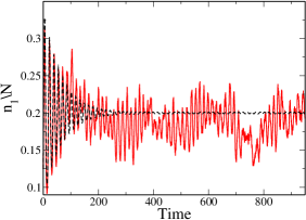
Figure 1: Temporal evolution of one of the species concentrations for a system composed by $4$ species and parameters set as $N=8190$, $r_{i}=10$ and $\alpha_{i}=\beta_{i}=1/64$ $\forall i$. The noisy (red online) line represents one stochastic realization thought the Gillespie algorithm gil76 ; gil77 , while the dashed black line shows the numerical solution of the deterministic system given by Eq. (4).

III.2 The $N^{-1}$ corrections

Finite size effects related to the $N^{-1}$ corrections result in the Fokker-Planck equation:

$$\frac{\partial\Pi}{\partial\tau}=-\sum_{i=1}^{k}\frac{\partial}{\partial\xi_{i}}\Big{[}A_{i}(\xi)\Pi\Big{]}+\frac{1}{2}\sum_{j=1}^{k}\sum_{i=1}^{k}\frac{\partial^{2}}{\partial\xi_{i}\partial\xi_{j}}\Big{[}b_{ij}\Pi\Big{]}$$ (6)

which governs the evolution of the distribution $\Pi(\cdot)$. Here $A_{i}(\boldsymbol{\xi})$ reads:

$$A_{i}(\boldsymbol{\xi})=(r_{i}\phi_{i-1}-r_{i+1}\phi_{i+1})\xi_{i}-r_{i+1}\phi_{i}\xi_{i+1}+r_{i}\phi_{i}\xi_{i-1}-\alpha_{i}\sum_{m=1}^{k}\xi_{m}-\beta_{i}\xi_{i},$$

while $b_{ij}$ stands for the element ${ij}$ of matrix $B$ defined as:

$$b_{ij}=\left\{\begin{array}[]{ll}r_{i+1}\phi_{i}\phi_{i+1}+r_{i}\phi_{i}\phi_{i-1}+\alpha_{i}(1-\sum_{m=1}^{k}\phi_{m})+\beta_{i}\phi_{i}&\quad\text{if}\quad i=j\\ -r_{i+1}\phi_{i}\phi_{i+1}&\quad\text{if}\quad j=i+1\\ -r_{i}\phi_{i-1}\phi_{i}&\quad\text{if}\quad j=i-1\\ 0&\quad\text{if}\quad|i-j|>1.\end{array}\right.$$

For the sake of clarity we shall introduce the matrix $M$ of elements $m_{ij}$ defined as:

$$m_{ij}=\left\{\begin{array}[]{ll}r_{i}\phi_{i-1}-r_{i+1}\phi_{i+1}-\alpha_{i}-\beta_{i}&\quad\text{if}\quad i=j\\ -r_{i+1}\phi_{i}-\alpha_{i}&\quad\text{if}\quad j=i+1\\ r_{i}\phi_{i}-\beta_{i}&\quad\text{if}\quad j=i-1\\ -\alpha_{i}&\quad\text{if}\quad|i-j|>1\end{array}\right.$$

and so rewrite $A_{i}$ as:

$$A_{i}=\sum_{j=1}^{k}m_{ij}\xi_{j}.$$

The Fokker-Planck equation (6) has been previously obtained in dauxois and shown to explain the regular oscillations displayed in direct stochastic simulations. The oscillations, in fact, materialize in a peak in the power spectrum of fluctuations which can be analytically calculated working in the equivalent context of the Langevin equation. Here, we take a different route and reconstruct the distribution of fluctuations through the calculation of the associated moments. To allow for analytical progress, we will assume again identical chemical reactions rates for all species, namely $r_{i}=r$, $\beta_{i}=\beta$ and $\alpha_{i}=\alpha$ $\forall i$. Moreover, we will focus on the fluctuations around the equilibrium and so require $\phi_{i}=\phi^{*}$ $\forall i$. Under these conditions the matrix $M$ is circulating and can be cast in the form:

$$M=\left[\begin{array}[]{rrrrrr}m_{0}&m_{1}&m_{2}&m_{2}&\ldots&m_{3}\\ m_{3}&m_{0}&m_{1}&m_{2}&\ldots&m_{2}\\ m_{2}&m_{3}&m_{0}&m_{1}&\ldots&m_{2}\\ \ldots&\ldots&\ldots&\ldots&\ldots&\ldots\\ m_{1}&m_{2}&m_{2}&m_{2}&\ldots&m_{0}\\ \end{array}\right].$$

with $m_{0}=-\alpha-\beta$, $m_{1}=-r\phi^{*}-\alpha$, $m_{2}=-\alpha$, and $m_{3}=r\phi^{*}-\alpha$. The $k\times k$ matrix reads instead:

$$B=\left[\begin{array}[]{rrrrrrr}b_{0}&b_{1}&0&\ldots&0&b_{1}\\ b_{1}&b_{0}&b_{1}&\ldots&0&0\\ 0&b_{1}&b_{0}&\ldots&0&0\\ \ldots&\ldots&\ldots&\ldots&\ldots&\ldots\\ b_{1}&0&0&\ldots&b_{1}&b_{0}\\ \end{array}\right]$$

where $b_{0}=2r\phi^{*}\phi^{*}+\alpha(1-k\phi^{*})+\beta\phi^{*}$, and $b_{1}=-r\phi^{*}\phi^{*}$.

We recall that the solution of the Fokker–Planck equation (6) is a multivariate Gaussian which is univocally characterized by the associated families of first and second moments. Working within this setting, it is hence sufficient to derive the analytical equations that control the time evolution of the first two moments of the distribution. We will in particular provide closed analytical expressions for the asymptotic moments and draw a direct comparison with the numerical experiments.

IV Analytical estimates of the fluctuations distribution moments

Define the moment of order $p$ for $\xi_{i}$ the quantity

$$\langle\xi_{i}^{p}\rangle=\int\Pi(\boldsymbol{\xi})\xi_{i}^{p}d\boldsymbol{\xi}$$

Let us illustrate the analytical procedure that is here adopted, with reference to $\langle\xi_{i}^{2}\rangle$. To this end we start from Eq. (6) and multiply it on both sides by the factor $\xi_{i}^{2}$. Integrating over $\mathbb{R}^{k}$ in $d\boldsymbol{\xi}=(d\xi_{1},d\xi_{2},...,d\xi_{k})$, yields:

$$\int\xi_{i}^{2}\frac{\partial}{\partial\tau}\Pi(\boldsymbol{\xi},\tau)d\boldsymbol{\xi}=\int\xi_{i}^{2}\sum_{i}\frac{\partial}{\partial\xi_{i}}A_{i}(\boldsymbol{\xi})\Pi(\boldsymbol{\xi},\tau)d\boldsymbol{\xi}+\int\xi_{i}^{2}\frac{1}{2!}\sum_{i,j}\frac{\partial^{2}}{\partial\xi_{i}\partial\xi_{j}}b_{i,j}(\boldsymbol{\xi})\Pi(\boldsymbol{\xi},\tau)d\boldsymbol{\xi}.$$ (7)

Consider the right hand side of Eq. (7) and operate two successive integrations by parts. Just two terms survive, as it can be trivially argued for. Hence, bringing out the time derivative from the integral at the left hand side of Eq. (7), the sought equation for the second moments reads:

$$\dot{\langle\xi_{i}^{2}\rangle}=2m_{i,i}\langle\xi_{i}^{2}\rangle+2m_{i,i-1}\langle\xi_{i}\xi_{i-1}\rangle+2m_{i,i+1}\langle\xi_{i}\xi_{i+1}\rangle+2m_{i,i+2}\langle\xi_{i}\xi_{i+2}\rangle+b_{i,i}$$ (8)

where $i=1,...,4$. Use has been made of the definitions of the coefficients $m_{ij}$. With analogous steps one immediately obtains the differential equation that governs the time evolution of quantity $\langle\xi_{i}\xi_{j}\rangle$:

$$\begin{split}\dot{\langle\xi_{i}\xi_{j}\rangle}=&m_{i,i}\langle\xi_{i}\xi_{i+1}\rangle+m_{i+1,i}\langle\xi_{i}^{2}\rangle+m_{i,i+1}\langle\xi_{i+1}^{2}\rangle+m_{i,i+2}\langle\xi_{i+1}\xi_{i+2}\rangle\\ &+m_{i+1,i+1}\langle\xi_{i}\xi_{i+1}\rangle+m_{i+1,i+2}\langle\xi_{i}\xi_{i+2}\rangle+m_{i+1,i}\langle\xi_{i}^{2}\rangle\\ &+m_{i,i+3}\langle\xi_{i+3}\xi_{i+1}\rangle+b_{i,i+1}.\end{split}$$ (9)

which, in practice, encodes the degree of temporal correlation between species $i$ and $j$. The picture is completed by providing the equations for the first moments which read:

$$\dot{\langle\xi_{i}\rangle}=m_{i,i}\langle\xi_{i}\rangle+m_{i,i-1}\langle\xi_{i-1}\rangle+\langle\xi_{i}\rangle m_{i,i+1}-m_{i,i+2}\langle\xi_{i+2}\rangle.$$

Taking into account all possible permutations of the involved indexes $i,j$, both ranging in the interval from $1$ to $4$, and recalling the Eq.s (8)–(9), one eventually obtains a closed system of ten coupled ordinary differential equations. For the simplified case $r_{i}=r$, $\alpha_{i}=\alpha$, $\beta_{i}=\beta$ $\forall i$, this latter can be cast in a compact form by introducing the matrix:

$$K=\left(\begin{array}[]{cccccccccc}2m_{0}&2m_{1}&2m_{2}&2m_{3}&0&0&0&0&0&0\\ m_{3}&2m_{0}&m_{1}&m_{2}&m_{1}&m_{1}&m_{2}&m_{3}&0&0\\ m_{2}&m_{3}&2m_{0}&m_{1}&0&m_{1}&0&m_{2}&m_{3}&0\\ m_{1}&m_{2}&m_{3}&2m_{0}&0&0&m_{1}&0&m_{2}&m_{3}\\ 0&2m_{3}&0&0&2m_{0}&2m_{1}&2m_{2}&0&0&0\\ 0&m_{2}&m_{3}&0&m_{3}&2m_{0}&m_{1}&m_{1}&m_{2}&0\\ 0&m_{1}&0&m_{3}&m_{2}&m_{3}&2m_{0}&0&m_{1}&m_{2}\\ 0&0&2m_{2}&0&0&2m_{3}&0&2m_{0}&2m_{1}&0\\ 0&0&m_{1}&m_{2}&0&m_{2}&m_{3}&m_{3}&2m_{0}&m_{1}\\ 0&0&0&2m_{1}&0&0&2m_{2}&0&2m_{3}&2m_{0}\\ \end{array}\right)$$

By further defining:

$$\boldsymbol{X}=\left[\langle\xi_{1}^{2}\rangle\quad\langle\xi_{1}\xi_{2}\rangle\quad\langle\xi_{1}\xi_{3}\rangle\quad\langle\xi_{1}\xi_{4}\rangle\quad\langle\xi_{2}^{2}\rangle\quad\langle\xi_{2}\xi_{3}\rangle\quad\langle\xi_{2}\xi_{4}\rangle\quad\langle\xi_{3}^{2}\rangle\quad\langle\xi_{3}\xi_{4}\rangle\quad\langle\xi_{4}^{2}\rangle\right]$$

and the vector

$$D=\left[b_{0}\quad b_{1}\quad 0\quad b_{1}\quad b_{0}\quad b_{1}\quad 0\quad b_{0}\quad b_{1}\quad b_{0}\right]$$

one gets

$$\dot{\boldsymbol{X}}=K\boldsymbol{X}+D\quad.$$

As anticipated, we focus in particular on the late time evolution of the system, i.e. when the fluctuations’ distribution has converged to its asymptotic form. This request translates into the mathematical condition $\dot{\boldsymbol{X}}=0$, which implies dealing with an algebraic system of equations. Given the peculiar structure of the problem, and by invoking a straightforward argument of symmetry , one can identify three families of independent unknowns, namely:

$$\begin{split}&\langle\xi_{1}^{2}\rangle=\langle\xi_{2}^{2}\rangle=\langle\xi_{3}^{2}\rangle=\langle\xi_{4}^{2}\rangle=:\Gamma_{1}\\ &\langle\xi_{1}\xi_{2}\rangle=\langle\xi_{1}\xi_{4}\rangle=\langle\xi_{2}\xi_{3}\rangle=\langle\xi_{3}\xi_{4}\rangle=:\Gamma_{2}\\ &\langle\xi_{1}\xi_{3}\rangle=\langle\xi_{2}\xi_{4}\rangle=:\Gamma_{3}.\end{split}$$ (10)

Closed analytical expressions for the unknowns $\Gamma_{1},\Gamma_{2}$ and $\Gamma_{3}$ as a function of the chemical parameters can be derived and take the form:

$$\Gamma_{1} = \frac{2b_{0}}{5\alpha}-\frac{b_{1}}{5\alpha}$$

$$\Gamma_{2} = -\frac{b_{0}}{10\alpha}+\frac{3b_{1}}{10\alpha}$$ (11)

$$\Gamma_{3} = -\frac{b_{0}}{10\alpha}-\frac{b_{1}}{5\alpha}$$

In deriving the above, we have assumed a further simplifying condition, namely $\alpha=\beta$. The adequacy of the predictions is tested in Fig. 2, where $\Gamma_{1}$ and $\Gamma_{2}$ are plotted versus the independent parameter $\alpha$. Recalling the explicit forms of $b_{0}$ and $b_{1}$ one can immediately appreciate that $\Gamma_{3}$ is indeed independent of $\alpha$. For this reason we here avoid to include $\Gamma_{3}$ in Fig. 2. One can moreover make use of the knowledge of the moments to reconstruct the profile of the distribution $\Pi(\boldsymbol{\xi})$. In particular, and due to the symmetry of the model, we solely focus on the marginal distribution $\Pi(\xi)=\Pi(\xi_{i})$ for $i=1,\ldots,4$. In practice, we project the distribution in a one-dimensional subspace by integrating over three out of four scalar independent variables $\xi_{i}$. In Fig. 3, a comparison between theory and stochastic simulations (relative to small $N$ values) is drawn. While the agreement is certainly satisfying, deviations from the predicted Gaussian profile manifest as the population size shrinks. As we shall demonstrate, these distortions, which materialize in a skewed distribution, can be successfully explained within an extended interpretative framework that moves from the van Kampen system size expansion. In the following section we will hence extend the calculation beyond the Gaussian approximation. In doing so we will operate in the general setting for $\alpha\neq\beta$, but then specialize on the choice $\alpha=\beta$ to drastically reduce the complexity of the inspected problem.

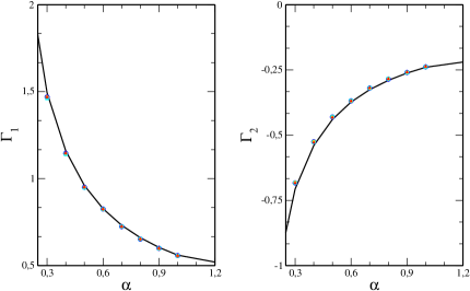
Figure 2: Plots of the moments $\Gamma_{1}$ and $\Gamma_{2}$ as functions of $\alpha$. The black lines show the theoretical predictions given by Eq. (11), while the (colored online) symbols represent the numerical simulations of the stochastic problem. Each symbol corresponds to a different component of the family according to (10). Parameters are set as $N=2000$, $\alpha=\beta$.

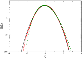
Figure 3: Comparison between the stationary marginal Gaussian distribution and the stochastic simulations (the y–axis has a logarithmic scale). The solid (red on line) line shows the theoretical prediction according to the van Kampen theory. The (green online) circles represent the numerical distribution for a system with $N=200$, while the (red online) triangles refer to a system with $N=2000$. For all the curves $r=10$, $\alpha=\beta=0.1$.

V Beyond the Gaussian approximation

We shall here go back to discussing the higher orders, $N^{-3/2}$ corrections to the Fokker-Planck equation. We will in particular consider the various terms that contribute to the generalized Fokker-Planck equation grouping them as a function of the order of the derivative involved.

The order $N^{-3/2}$ terms that involve the first derivatives can be expressed as:

$$\begin{split}\sum_{i=1}^{k}\Big{[}\frac{\partial}{\partial\xi_{i}}-\frac{\partial}{\partial\xi_{i+1}}\Big{]}r_{i+1}\xi_{i}\xi_{i+1}\Pi(\boldsymbol{\xi},\tau)&=\sum_{i=1}^{k}\frac{\partial}{\partial\xi_{i}}[r_{i+1}\xi_{i}\xi_{i+1}-r_{i}\xi_{i-1}\xi_{i}]\Pi(\boldsymbol{\xi},\tau)\\ &=-\sum_{i=1}^{k}\sum_{j=1}^{k}\frac{\partial}{\partial\xi_{i}}l_{ij}\xi_{i}\xi_{j}\Pi(\boldsymbol{\xi},\tau)\end{split}$$

where $l_{ij}$ are the elements of the $k\times k$ circulant matrix $L$ which, for $r_{i}=r\forall i$ reads:

$$L=\left(\begin{array}[]{cccccc}0&-r&0&\ldots&0&r\\ r&0&-r&\ldots&\ldots&0\\ 0&r&0&\ldots&\ldots&\ldots\\ [2.0]{6}\\ \ldots&\ldots&\ldots&\ldots&-r&0\\ 0&\ldots&\ldots&r&0&-r\\ -r&0&\ldots&0&r&0\\ \end{array}\right).$$

The order $N^{-3/2}$ contribution which depends on the second derivatives can be also expressed in a matricial form. In fact, we have:

$$\frac{1}{2}\Big{[}\frac{\partial^{2}}{\partial\xi_{i}^{2}}\beta_{i}\xi_{i}-\frac{\partial^{2}}{\partial\xi_{i}^{2}}\alpha_{i}\sum_{w}\xi_{w}+r_{i+1}\frac{\partial^{2}}{\partial\xi_{i}^{2}}(\xi_{i}\phi_{i+1}+\phi_{i}\xi_{i+1})+r_{i}\frac{\partial^{2}}{\partial\xi_{i}^{2}}(\xi_{i}\phi_{i-1}+\phi_{i}\xi_{i-1})\\ +2r_{i+1}\frac{\partial}{\partial\xi_{i}}\frac{\partial}{\partial\xi_{i+1}}(\xi_{i}\phi_{i+1}+\phi_{i}\xi_{i+1})\Big{]}\Pi(\boldsymbol{\xi},\tau)=\sum_{i=1}^{k}\sum_{j=1}^{k}\frac{\partial}{\partial\xi_{i}\partial\xi_{j}}d_{ij}$$

where the $k\times k$ matrix $D$ of elements $d_{ij}$, for $r_{i}=r$ $\forall i$, reads:

$$d_{ij}=\left\{\begin{array}[]{ll}\beta\xi_{i}-\alpha\sum_{w}\xi_{w}+r(\xi_{i}\phi^{*}+\xi_{i+1}\phi^{*})+r(\xi_{i}\phi^{*}+\xi_{i-1}\phi^{*})&\quad\text{if}\quad i=j\\ -r(\xi_{i}\phi^{*}+\xi_{i+1}\phi^{*})&\quad\text{if}\quad j=i+1\\ -r(\xi_{i}\phi^{*}+\xi_{i-1}\phi^{*})&\quad\text{if}\quad j=i-1\\ 0&\quad\text{otherwise}.\end{array}\right.$$

Finally, the third order derivatives contribute as:

$$\Big{[}-\frac{1}{3!}\frac{\partial^{3}}{\partial\xi_{i}^{3}}\alpha_{i}(1-\sum_{m}\phi_{m})+\frac{1}{3!}\Big{[}\frac{\partial}{\partial\xi_{i}}-\frac{\partial}{\partial\xi_{i+1}}\Big{]}^{3}r_{i+1}\phi_{i}\phi_{i+1}+\frac{1}{3!}\frac{\partial^{3}}{\partial\xi_{i}^{3}}\beta_{i}\phi_{i}\Big{]}\Pi(\boldsymbol{\xi},\tau)=-\sum_{i,j,w}\frac{\partial^{3}}{\partial\xi_{i}\partial\xi_{j}\partial\xi_{w}}e_{ijw}\Pi(\boldsymbol{\xi},\tau)$$

where, we introduced the matrix $E$ defined as:

$$e_{ijw}=\left\{\begin{array}[]{lll}r(\phi^{*})^{2}&\quad j=i&\quad w=i+1\\ r(\phi^{*})^{2}&\quad j=i-1&\quad w=i-1\\ r(\phi^{*})^{2}&\quad j=i+1&\quad w=i\\ -r(\phi^{*})^{2}&\quad j=i+1&\quad w=i+1\\ -r(\phi^{*})^{2}&\quad j=i&\quad w=i-1\\ -r(\phi^{*})^{2}&\quad j=i-1&\quad w=i\\ -[\beta\phi^{*}-\alpha(1-k\phi^{*})]&\quad i=j=w.&\phantom{i}\end{array}\right.$$

In conclusion, one gets the following equation for the distribution $\Pi(\boldsymbol{\xi},\tau)$ zamuner :

$$\frac{\partial\Pi(\boldsymbol{\xi},\tau)}{\partial\tau}=-\sum_{i=1}^{k}\frac{\partial}{\partial\xi_{i}}[A_{i}(\boldsymbol{\xi})\Pi(\boldsymbol{\xi},\tau)]+\frac{1}{2}\sum_{i,j=1}^{k}\frac{\partial^{2}}{\partial\xi_{i}\partial\xi_{j}}[b_{ij}\Pi(\boldsymbol{\xi},\tau)]-\frac{1}{N^{1/2}}\sum_{i=1}^{k}\frac{\partial}{\partial\xi_{i}}[C_{i}(\boldsymbol{\xi})\Pi(\boldsymbol{\xi},\tau)]\\ +\frac{1}{2N^{1/2}}\sum_{i,j=1}^{k}\frac{\partial^{2}}{\partial\xi_{i}\partial\xi_{j}}[d_{ij}(\boldsymbol{\xi})\Pi(\boldsymbol{\xi},\tau)]-\frac{1}{3!N^{1/2}}\sum_{i,j,w=1}^{k}\frac{\partial^{3}}{\partial\xi_{i}\partial\xi_{j}\partial\xi_{w}}[e_{ijw}\Pi(\boldsymbol{\xi},\tau)]$$ (12)

where:

$$C_{i}(\boldsymbol{\xi})=\sum_{j=1}^{k}l_{ij}\xi_{i}\xi_{j}.$$

We will refer to the latter as to the generalized Fokker–Planck equation. In the following section we will discuss the corrections to the Gaussian approximation as deduced by the above mathematical framework.

VI Non Gaussian corrections to the moments of the distribution

Starting from Eq. (12) we shall now assume $k=4$ and calculate the first three moments of the asymptotic distribution of the fluctuations around the mean field equilibrium. Clearly, the derivation can be in principle extended to evaluate the contribution of higher moments. The algebraic complexity of such an extension is however considerable and for this reason the third is the largest moment here characterized. The conclusions are nevertheless rather interesting as evaluating the third moment allows us to quantify the observed degree of skewness in the distribution of fluctuations.

When it comes to the first moment one gets:

$$\frac{d}{dt}\langle\xi_{i}\rangle=m_{i,i}\langle\xi_{i}\rangle+m_{i,i-1}\langle\xi_{i-1}\rangle+m_{i,i+1}\langle\xi_{i}\rangle+m_{i,i+2}\langle\xi_{i+2}\rangle+\frac{1}{N^{1/2}}[l_{i,i-1}\langle\xi_{i}\xi_{i-1}\rangle+l_{i,i+1}\langle\xi_{i}\xi_{i+1}\rangle]$$ (13)

This equation differs from the one obtained in section IV for the additional contribution

$$\frac{1}{N^{1/2}}[l_{i,i-1}\langle\xi_{i}\xi_{i-1}\rangle+l_{i,i+1}\langle\xi_{i}\xi_{i+1}\rangle]\quad.$$

Thanks to the symmetry of the system, which ultimately stems from having assumed $r_{i}=r$ $\forall i$, we can operate in a highly simplified framework. We notice in fact that the above term is function of the second moments, which have been estimated above and quantified as $\langle\xi_{i}\xi_{i+1}\rangle=\langle\xi_{i}\xi_{i-1}\rangle=\Gamma_{2}+o(1/\sqrt{N})$. Further we observe that $l_{i,i-1}=-l_{i,i+1}$. Hence the corrections to the Gaussian solution as exemplified in Eq. (13) contribute with an overall term of order $N^{-3/2}$, which can be legitimately neglected at this level of approximation. In conclusion the equation for the first moments is identical to that obtained in section IV.

Working in complete analogy, for the second moments we find:

$$\langle\dot{\xi_{i}^{2}}\rangle=2m_{i,i}\langle\xi_{i}^{2}\rangle+2m_{i,i+2}\langle\xi_{i}\xi_{i+2}\rangle+2m_{i,i+1}\langle\xi_{i}\xi_{i+1}\rangle+2m_{i,i-1}\langle\xi_{i}\xi_{i-1}\rangle+b_{i,i}+\frac{2}{N^{1/2}}[l_{i,i+1}\langle\xi_{i}^{2}\xi_{i+1}\rangle+l_{i,i-1}\langle\xi_{i}^{2}\xi_{i-1}\rangle]$$

for the variance of each involved species (recalling that the first moments are indeed null) and

$$\langle\dot{\xi_{i}\xi_{i+1}}\rangle = m_{i,i}\langle\xi_{i}\xi_{i+1}\rangle+m_{i,i+2}\langle\xi_{i+1}\xi_{i+2}\rangle+m_{i,i+1}\langle\xi_{i+1}^{2}\rangle+m_{i+1,i}\langle\xi_{i}^{2}\rangle+m_{i+1,i+1}\langle\xi_{i}\xi_{i+1}\rangle$$

$$+m_{i+1,i+2}\langle\xi_{i}\xi_{i+2}\rangle+m_{i,i+1}\langle\xi_{i}^{2}\rangle+m_{i,i+3}\langle\xi_{i+1}\xi_{i+3}\rangle+\frac{1}{2}b_{i,i+1}+\frac{1}{2}b_{i+1,i}$$

$$+\frac{1}{N^{1/2}}[l_{i,i+1}\langle\xi_{i}\xi_{i+1}^{2}\rangle+l_{i,i-1}\langle\xi_{i}\xi_{i-1}\xi_{i+1}\rangle+l_{i+1,i}\langle\xi_{i}^{2}\xi_{i+1}\rangle+l_{i+1,i+2}\langle\xi_{i}\xi_{i+2}\xi_{i+1}\rangle]$$

for the mutual correlation between distinct populations. The index $i$ ranges from $1$ to $4$. Again the extra contributions are limited to the terms stored in square brackets and prove to be negligible at this level of approximation. In fact the third order correlations therein involved should scale as $N^{-1/2}$ as requested by a simple consistency argument and as we shall prove a posteriori. Then, also in this case, thanks to the specific form of the matrix $L$, the additional contribution, stemming from third order moments, vanishes. We come hence to the conclusion that the second moments are identical to those calculated in the preceding section IV working within the Gaussian ansatz.

Let us now turn to calculating the third moments. After a lengthy derivation we end up with:

$$\langle\dot{\xi_{i}^{3}}\rangle=3m_{0}\langle\xi_{i}^{3}\rangle+3m_{3}\langle\xi_{i}^{2}\xi_{i-1}\rangle+3m_{2}\langle\xi_{i}^{2}\xi_{i+2}\rangle+3m_{1}\langle\xi_{i}^{2}\xi_{i+1}\rangle+3b_{0}\langle\xi_{i}\rangle+\frac{3}{N^{1/2}}[m_{4}\langle\xi_{i}^{2}\rangle\\ +m_{3}\langle\xi_{i}\xi_{i+1}\rangle+m_{3}\langle\xi_{i}\xi_{i-1}\rangle+3m_{2}\langle\xi_{i}\xi_{i+2}\rangle]+\frac{m_{5}}{N^{1/2}}+\frac{1}{N^{1/2}}[3r\langle\xi_{i}^{3}\xi_{i-1}\rangle-3r\langle\xi_{i}^{3}\xi_{i+1}\rangle]$$

where $m_{0}=-2\alpha$, $m_{1}=-\alpha-r/5$, $m_{2}=-\alpha$, $m_{3}=-\alpha+r/5$, $m_{4}=2r/5$, $m_{5}=m_{6}=0$, $m_{7}=-2r/5$, $m_{8}=r/25$ and $m_{9}=-r/5$. Here again, and as anticipated in the preceding discussion, we have chosen the simplifying setting with $\alpha=\beta$, which consequently implies $\phi^{*}=1/5$. Elaborating on the symmetry one can identify five families of independent moments, which obey to the above and the following differential equations:

$$\frac{d}{dt}\langle\xi_{i}^{2}\xi_{i-1}\rangle = 3m_{0}\langle\xi_{i}^{2}\xi_{i-1}\rangle+2m_{3}\langle\xi_{i}\xi_{i-1}^{2}\rangle+2m_{1}\langle\xi_{i}\xi_{i+1}\xi_{i-1}\rangle+2m_{2}\langle\xi_{i}\xi_{i-1}\xi_{i+2}\rangle+m_{3}\langle\xi_{i}^{2}\xi_{i+2}\rangle$$

$$+m_{1}\langle\xi_{i}^{3}\rangle+m_{2}\langle\xi_{i}^{2}\xi_{i+1}\rangle+b_{0}\langle\xi_{i-1}\rangle+2b_{1}\langle\xi_{i}\rangle$$

$$+\frac{1}{N^{1/2}}[m_{3}\langle\xi_{i-1}^{2}\rangle+m_{6}\langle\xi_{i}\xi_{i+1}\rangle+m_{3}\langle\xi_{i+1}\xi_{i-1}\rangle+m_{2}\langle\xi_{i-1}\xi_{i+2}\rangle+m_{7}\langle\xi_{i}^{2}\rangle]$$

$$-\frac{m_{8}}{N^{1/2}}+\frac{1}{N^{1/2}}[-2r\langle\xi_{i-1}\xi_{i}^{2}\xi_{i+1}\rangle+2r\langle\xi_{i-1}^{2}\xi_{i}^{2}\rangle+r\langle\xi_{i}^{2}\xi_{i-1}\xi_{i+2}\rangle-r\langle\xi_{i}^{3}\xi_{i-1}\rangle]$$

and

$$\frac{d}{dt}\langle\xi_{i}^{2}\xi_{i+1}\rangle = 3m_{0}\langle\xi_{i}^{2}\xi_{i+1}\rangle+2m_{3}\langle\xi_{i}\xi_{i-1}\xi_{i+1}\rangle+2m_{1}\langle\xi_{i}\xi_{i+1}^{2}\rangle+2m_{2}\langle\xi_{i}\xi_{i+1}\xi_{i+2}\rangle$$

$$+m_{3}\langle\xi_{i}^{3}\rangle+m_{1}\langle\xi_{i}^{2}\xi_{i+2}\rangle+m_{2}\langle\xi_{i}^{2}\xi_{i-1}\rangle+b_{0}\langle\xi_{i+1}\rangle+2b_{1}\langle\xi_{i}\rangle$$

$$+\frac{1}{N^{1/2}}[m_{3}\langle\xi_{i+1}^{2}\rangle+m_{6}\langle\xi_{i}\xi_{i+1}\rangle+m_{3}\langle\xi_{i+1}\xi_{i+3}\rangle+m_{2}\langle\xi_{i+1}\xi_{i+2}\rangle+m_{7}\langle\xi_{i}^{2}\rangle]$$

$$+\frac{m_{8}}{N^{1/2}}+\frac{1}{N^{1/2}}[-2r\langle\xi_{i+1}^{2}\xi_{i}^{2}\rangle+2r\langle\xi_{i-1}\xi_{i+1}\xi_{i}^{2}\rangle+r\langle\xi_{i}^{3}\xi_{i+1}\rangle-r\langle\xi_{i}^{2}\xi_{i+1}\xi_{i+2}\rangle]$$

for adjacent populations with respect to the assumed ordering. For next–to–neighbors correlation one gets:

$$\frac{d}{dt}\langle\xi_{i}^{2}\xi_{i+2}\rangle = 3m_{0}\langle\xi_{i}^{2}\xi_{i+2}\rangle+2m_{3}\langle\xi_{i}\xi_{i-1}\xi_{i+2}\rangle+2m_{1}\langle\xi_{i}\xi_{i+1}\xi_{i+2}\rangle+2m_{2}\langle\xi_{i}\xi_{i+2}^{2}\rangle+m_{3}\langle\xi_{i}^{2}\xi_{i+1}\rangle$$

$$+m_{1}\langle\xi_{i}^{2}\xi_{i-1}\rangle+m_{2}\langle\xi_{i}^{3}\rangle+b_{0}\langle\xi_{i+2}\rangle+\frac{1}{N^{1/2}}[-r\langle\xi_{i}^{2}\xi_{i+1}\xi_{i+2}\rangle+r\langle\xi_{i-1}\xi_{i+2}\xi_{i}^{2}\rangle]$$

$$+\frac{1}{N^{1/2}}[m_{2}\langle\xi_{i+2}^{2}\rangle+m_{4}\langle\xi_{i}\xi_{i+2}\rangle+m_{3}\langle\xi_{i-1}\xi_{i+2}\rangle+m_{3}\langle\xi_{i+1}\xi_{i+2}\rangle]\quad.$$

Finally, for correlations that involve three distinct species, we find:

$$\frac{d}{dt}\langle\xi_{i}\xi_{i+1}\xi_{i-1}\rangle = 3m_{0}\langle\xi_{i}\xi_{i+1}\xi_{i-1}\rangle+m_{3}\langle\xi_{i+1}\xi_{i-1}^{2}\rangle+m_{1}\langle\xi_{i+1}^{2}\xi_{i-1}\rangle+m_{2}\langle\xi_{i+2}\xi_{i+1}\xi_{i-1}\rangle$$

$$+m_{3}\langle\xi_{i}^{2}\xi_{i-1}\rangle+m_{1}\langle\xi_{i}\xi_{i+2}\xi_{i-1}\rangle+m_{3}\langle\xi_{i}\xi_{i+1}\xi_{i+2}\rangle+m_{2}\langle\xi_{i}\xi_{i-1}^{2}\rangle+m_{1}\langle\xi_{i}^{2}\xi_{i+1}\rangle$$

$$+m_{2}\langle\xi_{i}\xi_{i+1}^{2}\rangle+b_{1}\langle\xi_{i-1}\rangle+b_{1}\langle\xi_{i+1}\rangle+\frac{1}{N^{1/2}}[m_{9}\langle\xi_{i-1}\xi_{i}\rangle+m_{9}\langle\xi_{i+1}\xi_{i}\rangle$$

$$+m_{7}\langle\xi_{i-1}\xi_{i+1}\rangle]+\frac{1}{N^{1/2}}[-r\langle\xi_{i+1}^{2}\xi_{i}\xi_{i-1}\rangle+r\langle\xi_{i+1}\xi_{i}\xi_{i-1}^{2}\rangle].$$

Clearly, the fourth moments enter the equation for the third ones. To close the system and so enable for quantitative predictions, we can estimate the zero–th order contribution to the fourth moments by recalling the Gaussian solution as obtained in Section IV and neglecting the $1/\sqrt{N}$ terms. In formula:

$$\langle\xi_{i}^{4}\rangle = 3(\langle\xi_{i}^{2}\rangle)^{2}$$

$$\langle\xi_{i}^{3}\xi_{j}\rangle = 3\langle\xi_{i}^{2}\rangle\langle\xi_{i}\xi_{j}\rangle$$

$$\langle\xi_{i}^{2}\xi_{j}^{2}\rangle = \langle\xi_{i}^{2}\rangle\langle\xi_{j}^{2}\rangle+2(\langle\xi_{i}\xi_{j}\rangle)^{2}$$

$$\langle\xi_{i}^{2}\xi_{j}\xi_{k}\rangle = \langle\xi_{i}^{2}\rangle\langle\xi_{j}\xi_{k}\rangle+2\langle\xi_{i}\xi_{j}\rangle\langle\xi_{i}\xi_{k}\rangle.$$

The above quantities can be analytically estimated at equilibrium and expressed as a function of respectively $\Gamma_{1}$, $\Gamma_{2}$, $\Gamma_{3}$, as derived in section VI.

VI.1 The asymptotic evolution of the third moments

Let us now write down the system of differential equations that controls the dynamics of the five independent families of moments of order three . Such a system takes the form

$$\dot{\boldsymbol{X}}=V\boldsymbol{X}+S$$ (14)

where $\boldsymbol{X}$ is

$$\boldsymbol{X}=\left[\langle\xi_{i}^{3}\rangle\quad\langle\xi_{i}^{2}\xi_{i+1}\rangle\quad\langle\xi_{i}^{2}\xi_{i-1}\rangle\quad\langle\xi_{i}^{2}\xi_{i+2}\rangle\quad\langle\xi_{i}\xi_{i+1}\xi_{i-1}\rangle\right]$$ (15)

and the matrix of coefficients $V$ reads:

$$V=\left(\begin{array}[]{ccccc}3m_{0}&3m_{1}&3m_{3}&3m_{2}&0\\ m_{3}&3m_{0}&2m_{1}+m_{2}&m_{1}&2m_{3}+2m_{2}\\ m_{1}&2m_{3}+m_{2}&3m_{0}&m_{3}&2m_{1}+2m_{2}\\ m_{2}&m_{3}&m_{1}&3m_{0}+2m_{2}&2m_{3}+2m_{1}\\ 0&m_{2}+m_{1}&m_{3}+m_{2}&m_{3}+m_{1}&3m_{0}+m_{1}+m_{3}+m_{2}\\ \end{array}\right).$$

Finally the vector $S$ is:

$$S=1/\sqrt{N}\left[s_{1}\quad s_{2}\quad s_{3}\quad s_{4}\quad s_{5}\right]$$

where:

$$s_{1} = 3m_{4}\Gamma_{1}+6m_{3}\Gamma_{2}+3m_{2}\Gamma_{3}$$

$$s_{2} = m_{3}\Gamma_{1}+m_{7}\Gamma_{1}+m_{3}\Gamma_{3}+m_{2}\Gamma_{2}+m_{6}\Gamma_{2}+m_{8}+[-2r(\Gamma_{1})^{2}+2r\Gamma_{3}\Gamma_{1}-2r\Gamma_{3}\Gamma_{2}+2r\Gamma_{1}\Gamma_{2}]$$

$$s_{3} = m_{3}\Gamma_{1}+m_{7}\Gamma_{1}+m_{3}\Gamma_{3}+m_{2}\Gamma_{2}+m_{6}\Gamma_{2}-m_{8}+[2r(\Gamma_{1})^{2}-2r\Gamma_{1}\Gamma_{3}+2r\Gamma_{3}\Gamma_{2}-2r\Gamma_{1}\Gamma_{2}]$$

$$s_{4} = m_{4}\Gamma_{3}+2m_{3}\Gamma_{2}+m_{2}\Gamma_{1}$$

$$s_{5} = m_{7}\Gamma_{3}+2m_{9}\Gamma_{2}\quad.$$

We now turn to numerical simulations to validate the correctness of the theory. Stochastic simulations are performed for small systems ($N=200$) and the time evolution of the third moments is monitored for each of the considered species and by varying the parameter $\alpha$, while keeping $r$ unchanged. Results are displayed in Fig.s 4–8, where the simulations outcome (symbols) are compared to the theory predictions. The agreement has to be considered satisfactory, a conclusion which a posteriori validates the theory assumptions and in particular confirms the predictive ability of the van Kampen expansion beyond the Gaussian approximation Grima ; vk .

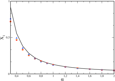
Figure 4: Plots of $X_{1}$ (see Eq. (15)) as functions of the parameter $\alpha$, for a system with $\beta=\alpha$, $N=200$ and $r=10$. The solid black lines represent the numerical solution of the system (14), while the symbols refer to the stochastic simulations (each of the four symbols is associated to a different species).

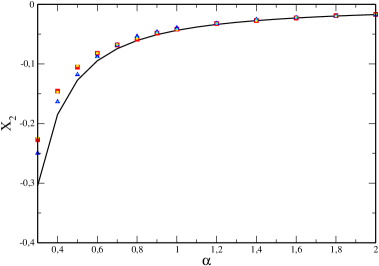
Figure 5: Plots of $X_{2}$ as functions of the parameter $\alpha$. For the parameters’ setting and the explanation of the symbols see caption of Fig. 4.

Figure 6: Plots of $X_{3}$ as functions of the parameter $\alpha$. For the parameters’ setting and the explanation of the symbols see caption of Fig. 4.

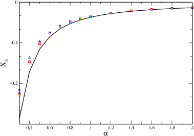
Figure 7: Plots of $X_{4}$ as functions of the parameter $\alpha$. For the parameters’ setting and the explanation of the symbols see caption of Fig. 4.

Figure 8: Plots of $X_{5}$ as functions of the parameter $\alpha$. For the parameters’ setting and the explanation of the symbols see caption of Fig. 4.

VII Conclusion

The study of an extended set of autocatalytic reactions proves interesting in many respects. The system self-organizes at the macroscopic level, both in space and time, as follows a non linear resonance mechanism that enhances the stochastic fluctuations stemming from the finite size. The spontaneous emergence of collective patterns, as well as regular time oscillations in such a system, was recently addressed dauxois ; deanna by analyzing in detail the underlying stochastic process via the celebrated van Kampen expansion, truncated at the Gaussian oder of approximation. In deanna , it was also speculated that the intrinsic ability of the autocatalytic systems to drive self-organized structures might have played a role in the evolutionary selection of efficient cells, starting from minimalistic protocells entities. It was in fact argued that oscillatory, spatially extended patterns, might have resonate with the innate ability of a vesicle container to divide in two. One could imagine that the oscillations trigger the splitting event and thus favor a natural synchronization between the fission of the vesicle and the rate of production of the genetic material stored inside, which needs to be passed to the next generation offspring.

Besides these highly speculative considerations, which deserve to be carefully checked within a self-consistent picture, we are here interested in extending the perturbative calculation beyond the second order approximation and challenge its adequacy in capturing the deviation from the idealized Gaussian behavior. Recent support on the validity of the van Kampen higher orders calculation have been provided by Grima and collaborators Grima . We here bring one more evidence on the accuracy of the procedure within a rather complex model, where different species are simultaneously made to interact. Numerical simulations performed in a stochastic setting with modest sizes of the population involved, so to magnify the role played by finite size corrections, confirm the correctness of the theory predictions. Due to the complexity of the proposed model, it is not possible to evaluate a large gallery of successive moments and so reconstruct the full distribution of fluctuations. The analysis is hence limited to the third moment, which however quantifies the degree of skewness of the recorded fluctuations. In a separate contribution cianci_voter , we will return on the issue of the validity of the van Kampen ansatz, working within a considerably simpler model that enables us to explicitly calculate all the moments of the distribution at any order of the expansion. We are hence able to recover a general and exact analytical solution that, we anticipate, agrees very well with the simulations, inline with the conclusion of this work.

References

(1)B. Alberts et al. Molecular Biology of the Cell,
(Garland Science, New York, 2007). Fifth edition.
(2)H. J. Morowitz, B. Heinz, and D. W. Deamer.
Orig. Life Evol. Biosph.18, 281 (1988).
(3)D. W. Deamer. Orig. Life Evol. Biosph.17, 3
(1986).
(4)P. L. Luisi. The Emergence of Life, (Cambridge
University Press, Cambridge, 2006).
(5)M. Eigen. Naturwissenschaften58, 465 (1971).
(6)Y. Togashi and K. Kaneko. Phys. Rev. Lett.86,
2459 (2001); Y. Togashi and K. Kaneko. J. Phys. Soc. Jpn.72,
62 (2003).
(7) T. Dauxois, F. Di Patti, D. Fanelli, and A. J. McKane.
Phys. Rev. E79, 036112 (2009).
(8) P. de Anna, F. Di Patti, D. Fanelli, A. McKane, T. Dauxois,
Phys. Rev. E81, 056110 (2009).
(9)N. G. van Kampen. Stochastic Processes in Physics and
Chemistry (Elsevier, Amsterdam, 2007). Third edition.
(10) C. W. Gardiner. Handbook of Stochastic Methods
(Springer-Verlag, Berlin, 2004). Third edition.
(11) R. Grima Phys. Rev. Lett.102, 218103 (2009);
R. Grima, BMC Systems Biology3 101, 2009; P. Thomas, A. V. Staube, R. Grima,
J. Chem. Phys.133, 195101 (2010); R. Grima,
J. Chem. Phys.133, 035101 (2010).
(12)H. Risken, H. D. Vollmer. Z. Physik B35, 313 (1979).
(13)D. T. Gillespie. J. Comput. Phys.22, 403 (1976).
(14)D. T. Gillespie. J. Phys. Chem.81, 2340 (1977).
(15) S. Zamuner, Tesi Di Laurea, University of Padua (2009).
(16) C. Cianci, F. Di Patti, D. Fanelli, submitted to Phys. Rev. Lett. (2011).