The NLO QCD Corrections to $B_{c}$ Meson Production in $Z^{0}$ Decays

Abstract

The decay width of $Z^{0}$ to $B_{c}$ meson is evaluated at the next-to-leading order(NLO) accuracy in strong interaction. Numerical calculation shows that the NLO correction to this process is remarkable. The quantum chromodynamics(QCD) renormalization scale dependence of the results is obviously depressed, and hence the uncertainties lying in the leading order calculation are reduced.

PACS number(s): 13.85.Ni, 14.40.Nd, 12.39.Jh, 12.38.Bx.

I Introduction

$B_{c}$ meson has been attracting lots of attention in recent years. As the sole heavy quark meson that contains two different heavy flavors, its unique property attracts more and wide interests. Ever since its first discovery at the TEVATRON CDF , till now, various investigations on its production and decays have been carried out in aspects of theory Had1 ; Had2 ; Had3 and experiment CDF ; Ex1 ; Ex2 . $B_{c}$ meson provides an excellent platform for testing the Standard Model(SM) and effective theories, e.g., to see whether non-relativistic QCD(NRQCD) NRQCD is suitable for such system or not. In foreseeable near future, the $B_{c}$ physics study at the Large Hadron Collider(LHC) will tell us more about the nature of this special heavy bound system.

Of the $B_{c}$ meson production, apart from the direct ones, the indirect yields, like in top Top and $Z^{0}$ Z1 ; Z2 ; Z3 decays, are also important sources. The process of $Z^{0}$ decays to $B_{c}$ has an advantage of low background, but also with the disadvantage of low production rate, which prompts the LEP-I experiment unable to observe the $B_{c}$ signature Z1 . In the future, if a high luminosity, $10^{34}cm^{-2}s^{-1}$ or higher, electron-position collider, e.g. Internal Linear Collider(ILC) ILC , can set up, it would then be possible to study the $B_{c}$ meson indirect production in $Z^{0}$ decays. As estimated by Ref.GigaZ , there would be $10^{9}\sim 10^{10}$ $Z^{0}$ events produced each year at the ILC. Such kind of high luminosity collider, the so-called “Z factory” Zfac , will provide new opportunities for both electroweak study and hadron physics.

The indirect production of $B_{c}$ meson in $Z^{0}$ decays was evaluated by several groups at the leading order(LO) in strong interaction Z1 ; Z2 ; Z3 . It is well-known that in charm- and bottom-quark energy regions, the higher order corrections of strong interaction are usually big, sometimes even huge. In order to make a more solid prediction on the $B_{c}$ production in $Z^{0}$ decays, and to depress the energy scale dependence lying at the LO calculation, an evaluation on the next-to-leading order(NLO) correction is necessary, which is the aim of this work.

The paper is organized as follows: after the Introduction, in section II we repeat the leading order calculation on the $Z^{0}$ to $B_{c}$ decay width. In section III, the NLO virtual and real QCD corrections to Born level result are performed. In section IV, the numerical calculation for the process at NLO accuracy is done. The last section is remained for summary and conclusions.

II Calculation of The Born Level Decay Width

At the leading order in $\alpha_{s}$, there are four Feynman Diagrams for $B_{c}$ production in $Z^{0}$ decays, the $Z^{0}(p_{1})\rightarrow{B}_{c}(p_{0})+\bar{c}(p_{5})+b(p_{6})$, as shown in Fig.1. The momentum of each particle is assigned as: $p_{1}=p_{Z}$, $p_{3}=p_{\bar{b}}$, $p_{4}=p_{c}$, $p_{5}=p_{\bar{c}}$, $p_{6}=p_{b}$, $p_{0}=p_{3}+p_{4}$, $p_{3}=\frac{m_{b}}{m_{c}}p_{4}$. For $b$ and $c$ quark hadronization to ${B}_{c}$ meson, we employ the following commonly used projection operator

$$v(p_{3})\,\overline{u}(p_{4}) \longrightarrow {1\over 2\sqrt{2}}i\gamma_{5}(\not\!p_{0}+m_{b}+m_{c})\,\times\left({1\over\sqrt{(m_{b}+m_{c})/2}}~{}\psi_{{B}_{c}}(0)\right)\otimes\left({{\bf 1}_{c}\over\sqrt{N_{c}}}\right)$$ (1)

Here, ${\bf 1}_{c}$ stands for the unit color matrix, and $N_{c}=3$ for QCD. The nonperturbative parameter $\psi_{{B}_{c}}(0)$ is the Schrödinger wave function at the origin of the $\bar{b}c$ bound states. In our calculation, the non-relativistic relation $m_{{B}_{c}}=m_{b}+m_{c}$ is also adopted.

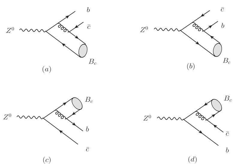
Figure 1: The leading order Feynman diagrams for ${B}_{c}$ production in $Z^{0}$ decays.

The LO amplitudes for ${B}_{c}$ production can then be readily obtained with above preparations. They are:

$${\cal M}_{a}=\frac{\pi\alpha_{s}g\psi_{{B}_{c}}(0)C_{F}\delta_{jk}}{6\sqrt{3m_{{B}_{c}}}\cos{\theta_{W}}}~{}\bar{u}(p_{6})\gamma_{\mu}\frac{\not\!\epsilon(p_{1})[(4\sin^{2}{\theta_{W}}-3)+3\gamma_{5}]}{(\not\!p_{1}-\not\!p_{3}-m_{b})({p_{4}+p_{5}})^{2}}~{}i\gamma_{5}(\not\!p_{0}+m_{{B}_{c}})\gamma^{\mu}v(p_{5})\;,$$ (2)

$${\cal M}_{b}=\frac{\pi\alpha_{s}g\psi_{{B}_{c}}(0)C_{F}\delta_{jk}}{6\sqrt{3m_{{B}_{c}}}\cos{\theta_{W}}}~{}\bar{u}(p_{6})\gamma^{\mu}~{}i\gamma_{5}(\not\!p_{0}+m_{{B}_{c}})\frac{\not\!\epsilon(p_{1})[(8\sin^{2}{\theta_{W}}-3)+3\gamma_{5}]}{({p_{3}+p_{6}})^{2}(\not\!p_{1}-\not\!p_{4}-m_{c})}\gamma_{\mu}v(p_{5})\;,$$ (3)

$${\cal M}_{c}=\frac{\pi\alpha_{s}g\psi_{{B}_{c}}(0)C_{F}\delta_{jk}}{6\sqrt{3m_{{B}_{c}}}\cos{\theta_{W}}}~{}\bar{u}(p_{6})\gamma^{\mu}~{}i\gamma_{5}(\not\!p_{0}+m_{{B}_{c}})\gamma_{\mu}\frac{\not\!\epsilon(p_{1})[(8\sin^{2}{\theta_{W}}-3)+3\gamma_{5}]}{(\not\!p_{1}-\not\!p_{5}-m_{c})({p_{3}+p_{6}})^{2}}v(p_{5})\;,$$ (4)

and

$${\cal M}_{d}=\frac{\pi\alpha_{s}g\psi_{{B}_{c}}(0)C_{F}\delta_{jk}}{6\sqrt{3m_{{B}_{c}}}\cos{\theta_{W}}}~{}\bar{u}(p_{6})\frac{\not\!\epsilon(p_{1})[(4\sin^{2}{\theta_{W}}-3)+3\gamma_{5}]}{({p_{4}+p_{5}})^{2}(\not\!p_{1}-\not\!p_{6}-m_{b})}\gamma^{\mu}~{}i\gamma_{5}(\not\!p_{0}+m_{{B}_{c}})\gamma_{\mu}v(p_{5})\;.$$ (5)

Here, $j$, $k$ are color indices, $C_{F}=4/3$ belongs to the $SU(3)$ color structure. $\theta_{W}$ is the Weinberg angle with the numerical value $\sin^{2}{\theta_{W}}=0.23$.

The Born amplitude of the processes shown in Fig.1 is then ${\cal M}_{Born}={\cal M}_{a}+{\cal M}_{b}+\mathcal{M}_{c}+\mathcal{M}_{d}$, and subsequently, the decay width at LO reads:

$$\mathrm{d}\Gamma_{Born}=\frac{1}{2m_{Z}}\frac{1}{3}\sum|{\cal M}_{Born}|^{2}\mathrm{d}\textmd{PS}_{3}\;.$$ (6)

Here, $\sum$ symbolizes the sum over polarizations and colors of the initial and final particles, $\frac{1}{3}$ comes from spin average of initial $Z^{0}$ meson, $\mathrm{d}\textmd{PS}_{3}$ stands for the integrals of three-body phase space, whose concrete form can be expressed as:

$$\mathrm{d}\textmd{PS}_{3}=\frac{1}{32\pi^{3}}\frac{1}{4m_{Z}^{2}}\mathrm{d}s_{2}\mathrm{d}s_{1}\;,$$ (7)

where $s_{1}=(p_{0}+p_{5})^{2}=(p_{1}-p_{6})^{2}$ and $s_{2}=(p_{5}+p_{6})^{2}=(p_{1}-p_{0})^{2}$ are Mandelstam variables. The upper and lower bounds of the above integration are

$$s_{1}^{max}= \frac{\sqrt{f[m_{Z}^{2},s_{2},m_{{B}_{c}}^{2}]\cdot f[s_{2},m_{c}^{2},m^{2}_{b}]}+[m_{Z}^{2}-s_{2}-(m_{b}+m_{c})^{2}](s_{2}+m_{c}^{2}-m^{2}_{b})}{2s_{2}}$$ (8)

$$+m_{{B}_{c}}^{2}+m_{c}^{2}\;,$$

$$s_{1}^{min}= -\frac{\sqrt{f[m_{Z}^{2},s_{2},m_{{B}_{c}}^{2}]\cdot f[s_{2},m_{c}^{2},m^{2}_{b}]}-[m_{Z}^{2}-s_{2}-(m_{b}+m_{c})^{2}](s_{2}+m_{c}^{2}-m^{2}_{b})}{2s_{2}}$$ (9)

$$+m_{{B}_{c}}^{2}+m_{c}^{2}$$

and

$$s_{2}^{max}=[m_{Z}-(m_{b}+m_{c})]^{2}\;,\;s_{2}^{min}=(m_{c}+m_{b})^{2}$$ (10)

with

$$f[x,y,z] = (x-y-z)^{2}-4yz\;.$$ (11)

III The Next-to-Leading Order Corrections

At the next-to-leading order, the $Z^{0}$ boson decay to ${B}_{c}$ includes the virtual and real QCD corrections to the leading order process. For the two kinds of vertices, $Z\rightarrow\bar{b}b$ and $Z\rightarrow\bar{c}c$, we need only to consider one of them, e.g. as shown in Figs.2-5, since they are similar. For the virtual corrections, the decay width at the NLO can be formulated as

$$\mathrm{d}\Gamma_{Virtual}=\frac{1}{2m_{Z}}\frac{1}{3}\sum 2\textmd{Re}({\cal M}_{Born}^{*}{\cal M}_{Virtual})\mathrm{d}\textmd{PS}_{3}\;.$$ (12)

In virtual corrections, the ultraviolet(UV) and infrared(IR) divergences exist universally. We use the dimensional regularization scheme to regularize both UV and IR divergences, similar as performed in Ref.DR , and use the relative velocity $v$ to regularize the Coulomb divergence vre . According to the power counting rule, the UV divergences exist merely in self-energy and triangle diagrams, which can be canceled by counter terms. The renormalization constants include $Z_{2}$, $Z_{3}$, $Z_{m}$, and $Z_{g}$, corresponding to quark field, gluon field, quark mass, and strong coupling constant $\alpha_{s}$, respectively. Here, in our calculation the $Z_{g}$ is defined in the modified-minimal-subtraction ($\mathrm{\overline{MS}}$) scheme, while for the other three the on-shell ($\mathrm{OS}$) scheme is adopted, which tells

$$\delta Z_{m}^{OS}=-3C_{F}\frac{\alpha_{s}}{4\pi}\left[\frac{1}{\epsilon_{UV}}-\gamma_{E}+\ln\frac{4\pi\mu^{2}}{m^{2}}+\frac{4}{3}+{\mathcal{O}}(\epsilon)\right]\;,$$

$$\delta Z_{2}^{OS}=-C_{F}\frac{\alpha_{s}}{4\pi}\left[\frac{1}{\epsilon_{UV}}+\frac{2}{\epsilon_{IR}}-3\gamma_{E}+3\ln\frac{4\pi\mu^{2}}{m^{2}}+4+{\mathcal{O}}(\epsilon)\right]\;,$$

$$\delta Z_{3}^{OS}=\frac{\alpha_{s}}{4\pi}\left[(\beta^{{}^{\prime}}_{0}-2C_{A})(\frac{1}{\epsilon_{UV}}-\frac{1}{\epsilon_{IR}})-\frac{4}{3}T_{f}(\frac{1}{\epsilon_{UV}}-\gamma_{E}+\ln\frac{4\pi\mu^{2}}{m_{c}^{2}})\right.$$

$$~{}~{}~{}~{}~{}~{}~{}~{}~{}~{}~{}~{}~{}~{}~{}~{}~{}~{}~{}~{}~{}~{}~{}~{}~{}~{}~{}~{}~{}~{}~{}~{}~{}~{}~{}\left.-\frac{4}{3}T_{f}(\frac{1}{\epsilon_{UV}}-\gamma_{E}+\ln\frac{4\pi\mu^{2}}{m_{b}^{2}})+{\mathcal{O}}(\epsilon)\right]\;,$$

$$\delta Z_{g}^{\overline{MS}}=-\frac{\beta_{0}}{2}\frac{\alpha_{s}}{4\pi}\left[\frac{1}{\epsilon_{UV}}-\gamma_{E}+\ln 4\pi+{\mathcal{O}}(\epsilon)\right]\;.$$ (13)

Here, the mass $m$ in $\delta Z_{m}^{OS}$ and $\delta Z_{2}^{OS}$ represents $m_{b}$ or $m_{c}$; $\beta_{0}=(11/3)C_{A}-(4/3)T_{f}n_{f}$ is the one-loop coefficient of the QCD beta function; $n_{f}=5$ is the number of active quarks in our calculation; and $\beta_{0}^{\prime}=(11/3)C_{A}-(4/3)T_{f}n_{lf}$ with $n_{lf}=3$ being the number of light-quark flavors; $C_{A}=3$ and $T_{F}=1/2$ attribute to the SU(3) group; $\mu$ is the renormalization scale. Note, since the terms related to $\delta\text{Z}_{3}^{OS}$ cancel with each other, the full NLO result is independent of the renormalization scheme of the gluon field.

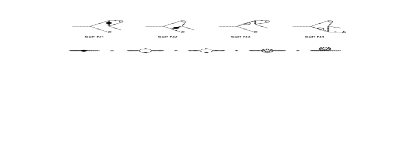
Figure 2: The self-energy diagrams in virtual corrections.

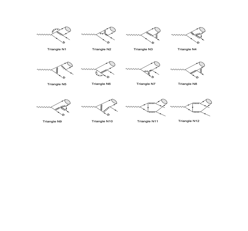
Figure 3: The triangle diagrams in virtual corrections.

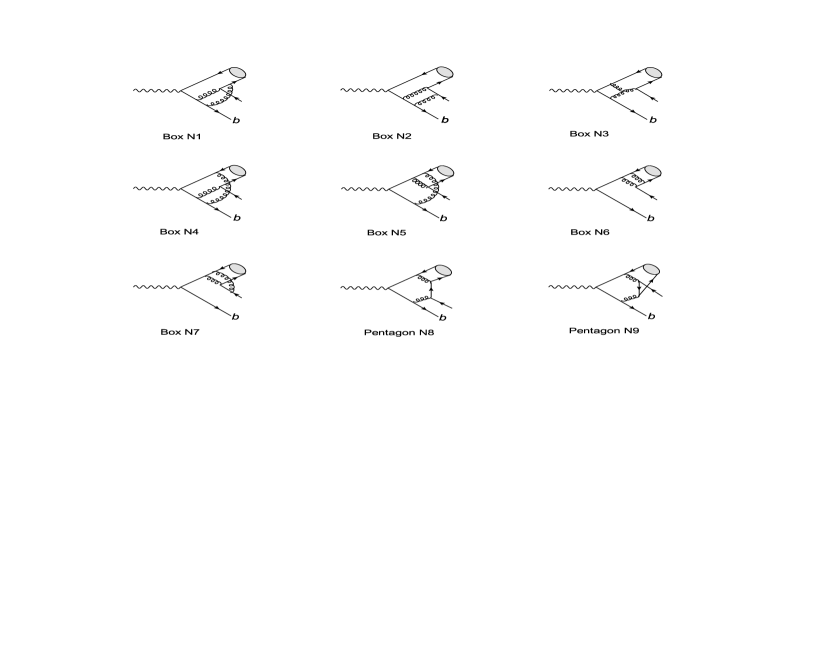
Figure 4: The box and pentagon diagrams in virtual corrections.

In dimensional regularization scheme, $\gamma_{5}$ is an object hard to handle; especially in the process that contains the vector-axial current, things become more complicated. In our work, we adopt the scheme provided in Ref.gamma5 , where the following rules must be obeyed:

I. the cyclicity is forbidden in traces involving odd number of $\gamma_{5}$.

II. For the certain diagrams that contribute to a process, we must write down the amplitudes starting at the same vertex, named the reading point.

III. As a special case of rule II, if the anomalous axial current exists, the reading point of the anomalous diagrams must be the axial vector vertex, in order to guarantee the conservation of the vector current.

By utilizing this rule in our process, the two anomalous diagrams denoted as $\mathrm{TriangleN11}$ and $\mathrm{TriangleN12}$ in Fig.3 are calculated, and the UV divergences in these two diagrams are canceled by each other. To deal with the $\gamma_{5}s$ except for what in anomalous diagrams, the cyclicity is employed to move the $\gamma_{5}s$ together and then are contracted by $\gamma_{5}^{2}=1$. Hence, if a trace contains even number of $\gamma_{5}$, there will be no $\gamma_{5}$ left. Otherwise, after the contraction of odd number of $\gamma_{5}$, one remains.

In the virtual correction, IR divergences remain in the triangle and box diagrams. Of all the triangle diagrams, only two have IR divergences, which are denoted by $\mathrm{TriangleN3}$ and $\mathrm{TriangleN8}$ in Fig.3. Of the diagrams in Fig.4, $\mathrm{BoxN3}$ has no IR divergence, $\mathrm{BoxN6}$ has merely the Coulomb singularity, $\mathrm{PentagonN8}$ has both a Coulomb singularity and ordinary IR divergence, and the remaining other diagrams have only the ordinary IR divergences. We find that the combinations of $\mathrm{BoxN1+BoxN4}$, $\mathrm{BoxN5+PentagonN9+TriangleN8}$, and $\mathrm{BoxN7+TriangleN3}$ are IR finite, while the remaining IR singularities in $\mathrm{BoxN2}$ and $\mathrm{BoxN8}$ are canceled by the corresponding parts in real corrections. The Coulomb singularities existing in $\mathrm{BoxN6}$ and $\mathrm{PentagonN8}$ can be regularized by the relative velocity $v$. The $\frac{1}{\epsilon}$ terms are renormalized by the counter terms of external quarks which form the ${B}_{c}$, while the $\frac{1}{v}$ term will be mapped onto the wave function of the concerned heavy meson. In the end, the IR and Coulomb divergences in virtual corrections can be expressed as

$$\mathrm{d}\Gamma_{virtual}^{IR,Coulomb}=\mathrm{d}\Gamma_{Born}\frac{8\alpha_{s}}{3\pi}\left[\frac{\pi^{2}}{v}-\frac{1}{\epsilon}+\frac{(m_{Z}^{2}+2m_{b}m_{c}-2p_{1}\cdot p_{0})x_{s}\ln x_{s}}{m_{b}m_{c}(1-x_{s}^{2})}\frac{1}{\epsilon}\right]$$ (14)

with $p_{1}=p_{Z}$, $p_{0}=p_{B_{c}}$ and $x_{s}=-\frac{1-\sqrt{1-4m_{b}m_{c}/(4m_{b}m_{c}+m_{Z}^{2}-2p_{1}\cdot p_{0})}}{1+\sqrt{1-4m_{b}m_{c}/(4m_{b}m_{c}+m_{Z}^{2}-2p_{1}\cdot p_{0})}}$. Here, in this work $\frac{1}{\epsilon}$ in fact represents $\frac{1}{\epsilon}-\gamma_{E}+\ln(4\pi\mu^{2})$.

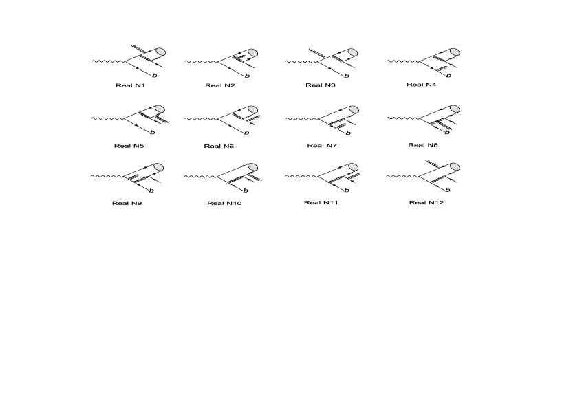
Figure 5: The real correction Feynman diagrams that contribute to the production of $B_{c}$.

Of the concerned process, there are $12$ different Feynman diagrams in real correction, as shown in Fig.5. Among them, $\mathrm{RealN2}$, $\mathrm{RealN3}$, $\mathrm{RealN8}$, and $\mathrm{RealN9}$ are IR-finite, meanwhile the combinations of $\mathrm{RealN1+RealN5}$ and $\mathrm{RealN10+RealN12}$ exhibit no IR singularities as well, due to the reason of gluon connecting to either $\bar{b}$ or $c$ quark of the final ${B}_{c}$ meson. The remaining diagrams, $\mathrm{RealN4}$, $\mathrm{RealN6}$, $\mathrm{RealN7}$, and $\mathrm{RealN11}$ are not IR singularity free. To regularize the IR divergence, we enforce a cut on the gluon momentum, the $p_{7}$. The gluon with energy $p_{7}^{0}<\delta$ is considered to be soft, while $p_{7}^{0}>\delta$ is thought to be hard. The $\delta$ is a small quantity with energy-momentum unit. In this way, the IR term of the decay width can then be written as:

$$\mathrm{d}\Gamma_{Real}^{IR}=\frac{1}{2m_{Z}}\frac{1}{3}\sum|{\cal M}_{Real}|^{2}\;\mathrm{d}\textmd{PS}_{4}\mid_{soft}\;,$$ (15)

where $\mathrm{d}\textmd{PS}_{4}$ is the four-body phase space integrants for real correction. Under the condition of $p_{7}^{0}<\delta$, in the Eikonal approximation we obtain

$$\mathrm{d}\textmd{PS}_{4}\mid_{soft}=\mathrm{d}\textmd{PS}_{3}\frac{d^{3}p_{7}}{(2\pi)^{3}2p_{7}^{0}}\mid_{p_{7}^{0}<\delta}\;.$$ (16)

In the small $\delta$ limit, the IR divergent terms in real correction can therefore be expressed as

$$\mathrm{d}\Gamma_{Real}^{IR}=\mathrm{d}\Gamma_{Born}\frac{8\alpha_{s}}{3\pi}\left\{\left(\frac{1}{\epsilon}-\ln(\delta^{2})\right)\left[1-\frac{(m_{Z}^{2}+2m_{b}m_{c}-2p_{1}\cdot p_{0})x_{s}\ln x_{s}}{m_{b}m_{c}(1-x_{s}^{2})}\right]+\rm{finite\;terms}\right\}.~{}~{}~{}$$ (17)

Here, the $\ln(\delta^{2})$ involved terms will be canceled by the $\delta$-dependent terms in the hard sector of real corrections. Comparing (17) with (14), it is obvious that the IR divergent terms in real and virtual corrections cancel with each other. In the case of hard gluons in real correction, the decay width reads

$$\mathrm{d}\Gamma_{Real}^{hard}=\frac{1}{2m_{Z}}\frac{1}{3}\sum|{\cal M}_{Real}|^{2}\;\mathrm{d}\textmd{PS}_{4}\mid_{hard}\;.$$ (18)

In this case, the phase space $\mathrm{d}\textmd{PS}_{4}\mid_{hard}$ can be expressed as

$$\int\mathrm{d}\textmd{PS}_{4}\mid_{hard}=\frac{2}{(4\pi)^{6}} \frac{\sqrt{(sy+m_{c}^{2}-m_{b}^{2})^{2}-4sym_{c}^{2}}}{y}\int_{{p_{0}}^{0}_{-}}^{{p_{0}}^{0}_{+}}\mathrm{d}{p_{0}}^{0}\int_{-1}^{1}\mathrm{d}\cos\theta_{c}\int_{0}^{2\pi}\mathrm{d}\phi_{c}$$ (19)

$$\times\left\{\int_{\delta}^{{p_{7}}^{0}_{-}}\mathrm{d}{p_{7}}^{0}\int_{y_{-}}^{y_{+}}\mathrm{d}y+\int_{{p_{7}}^{0}_{-}}^{{p_{7}}^{0}_{+}}\mathrm{d}{p_{7}}^{0}\int_{\frac{(m_{b}+m_{c})^{2}}{s}}^{y_{+}}\mathrm{d}y\right\}$$

with

$${p_{0}}^{0}_{-}=m_{b}+m_{c}\;,$$ (20)

$${p_{0}}^{0}_{+}=\frac{\sqrt{s}}{2}\;,$$ (21)

$${p_{7}}^{0}_{-}=\frac{s-2\sqrt{s}{p_{0}}^{0}}{2\sqrt{s}-2{p_{0}}^{0}+2\sqrt{|\overrightarrow{{p_{0}}}|}}\;,$$ (22)

$${p_{7}}^{0}_{+}=\frac{s-2\sqrt{s}{p_{0}}^{0}}{2\sqrt{s}-2{p_{0}}^{0}-2\sqrt{|\overrightarrow{{p_{0}}}|}}\;,$$ (23)

$$y_{-}=\frac{1}{s}[(\sqrt{s}-{p_{0}}^{0}-{p_{7}}^{0})^{2}-|\overrightarrow{{p_{0}}}|^{2}-({p_{7}}^{0})^{2}-2|\overrightarrow{p_{0}}|p_{7}^{0}]\;,$$ (24)

$$y_{+}=\frac{1}{s}[(\sqrt{s}-{p_{0}}^{0}-{p_{7}}^{0})^{2}-|\overrightarrow{{p_{0}}}|^{2}-({p_{7}}^{0})^{2}+2|\overrightarrow{p_{0}}|{p_{7}}^{0}]\;.$$ (25)

Here, $y$ is a dimensionless parameter defined as $y=(p_{1}-p_{0}-p_{7})^{2}/s$ with $\sqrt{s}=m_{Z}$, and $|\overrightarrow{p_{0}}|=\sqrt{({p_{0}}^{0})^{2}-m_{{B}_{c}}^{2}}\;.$ The sum of the soft and hard sectors gives the total contribution of real corrections, i.e., $\Gamma_{Real}=\Gamma_{Real}^{IR}+\Gamma_{Real}^{hard}$.

With the real and virtual corrections, we then obtain the total decay width of $Z$ boson to ${B}_{c}$ at the NLO accuracy of QCD

$$\Gamma_{total}=\Gamma_{Born}+\Gamma_{Virtual}+\Gamma_{Real}+{\mathcal{O}}(\alpha_{s}^{4})\;.$$ (26)

In above expression, the decay width is UV and IR finite. In our calculation the FeynArts feynarts was used to generate the Feynman diagrams, the amplitudes were generated by the FeynCalc feyncalc , and the LoopTools looptools was employed to calculate the Passarino-Veltman integrations. The numerical integrations of the phase space were performed by the MATHEMATICA.

IV Numerical results

To complete the numerical calculation, the following ordinarily accepted input parameters are taken into account:

$$m_{b}=4.9\;\textmd{GeV},\;m_{c}=1.5\;\textmd{GeV},\;m_{Z}=91\;\textmd{GeV},\;m_{W}=80\;\textmd{GeV},\;$$ (27)

$$G_{F}=1.1660\times 10^{-5}\;\mathrm{GeV}^{-2},\;g^{2}=\frac{8G_{F}m_{W}^{2}}{\sqrt{2}}=0.4221,$$ (28)

$$\psi_{{B}_{c}}(0)=\frac{R(0)}{\sqrt{4\pi}}=0.3616\;\textmd{GeV}^{\frac{3}{2}}.\;$$ (29)

Here, $R(0)$ is radial wave function at the origin of $B_{c}$ meson, which is estimated via potential model pot and $G_{F}$ is Fermi constant in weak interaction. The one loop result of strong coupling constant is taken into account in our calculation, i.e.

$$\alpha_{s}(\mu)=\frac{4\pi}{(11-\frac{2}{3}n_{f})\ln(\frac{\mu^{2}}{\Lambda_{QCD}^{2}})}\;.$$ (30)

With the above preparation, one can readily obtain the decay width of $Z^{0}$ to $B_{c}$ meson in NLO accuracy of pQCD. In practice, the renormalization scale $\mu$ may run from $2m_{b}$ to $m_{Z}/2$. At $\mu=2m_{b}$ and then $\alpha_{s}(2m_{b})=0.189$ with $\Lambda_{QCD}$ chosen to be $128~{}\mathrm{MeV}$, the LO and NLO decay widths of $Z^{0}\rightarrow B_{c}+\bar{c}b$ process are

$$\Gamma_{LO}(Z^{0}\rightarrow B_{c}+\bar{c}b)=72.31~{}\mathrm{keV}$$ (31)

and

$$\Gamma_{NLO}(Z^{0}\rightarrow B_{c}+\bar{c}b)=78.45~{}\mathrm{keV},$$ (32)

respectively. And, at the scale $\mu=m_{Z}/2$ and then $\alpha_{s}(m_{Z}/2)=0.140$, the corresponding results are

$$\Gamma_{LO}(Z^{0}\rightarrow B_{c}+\bar{c}b)=39.43~{}\mathrm{keV}$$ (33)

and

$$\Gamma_{NLO}(Z^{0}\rightarrow B_{c}+\bar{c}b)=62.53~{}\mathrm{keV}\;.$$ (34)

Our LO result agrees with that existing in the literature Ref.Z1 in case we take their inputs, i.e. $\alpha_{s}(m_{Z}/2)=0.150$ and $\psi_{{B}_{c}}(0)=0.369~{}\textmd{GeV}^{\frac{3}{2}}$. The above result indicates that at high energy scale, the NLO QCD correction to the decay width, or the $B_{c}$ production, is substantial. To see the scale dependence of the LO and NLO results, the decay width $\Gamma(\mu)$ and the ratio $\Gamma(\mu)/\Gamma(2m_{b})$ are shown in Fig.6 for $\mu$ varying from $2m_{b}$ to $m_{Z}/2$. Calculation results indicate that after including the NLO QCD corrections, as expected the energy scale dependence of the decay width $\Gamma(Z^{0}\rightarrow B_{c}+\bar{c}b)$ is reduced evidently.

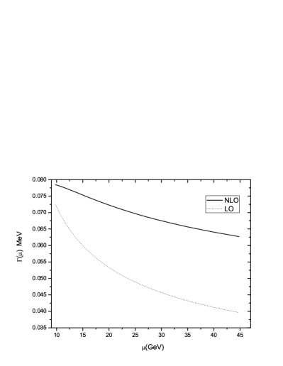
Figure 6: The decay width $\Gamma(\mu)$(left) and the ratio $\Gamma(\mu)/\Gamma(2m_{c})$(right) versus renormalization scale $\mu$ in $Z^{0}$ boson decays.

V Summary and Conclusions

In this work we have calculated the inclusive decay width of $Z^{0}$ boson to $B_{c}$ meson at the NLO accuracy of perturbative QCD. Supposing that there will be copious $Z^{0}$ data in the future at the “Z-factory”, our results are helpful to the precise study of $B_{c}$ physics, and may also tell how well non-relativistic model works for $B_{c}$ system.

Numerical results indicate that the NLO QCD correction slightly increases the LO result for the process $Z^{0}\rightarrow{B}_{c}+\bar{c}+b$ when $\mu$ is at the low energy scale of $2m_{b}$, while it becomes huge, even comparable to the LO result, when $\mu$ runs to the scale of $m_{Z}/2$. We find that the energy scale dependence of the decay width is depressed, as it should be, when the next-to-leading order correction is taken into account, which means the uncertainties in the theoretical estimation are reduced.

Acknowledgments

This work was supported in part by the National Natural Science Foundation of China(NSFC) and by the CAS Key Projects KJCX2-yw-N29 and H92A0200S2.

References

• (1) CDF Collaboraten, F. Abe, et al., Phys. Rev. Lett. 81, 2432 (1998); Phys. Rev. D58, 112004 (1998).
• (2) K. Cheung, Phys. Lett. B472, 408 (2000); Chao-Hsi Chang, Yu-Qi Chen and R. J. Oakes, Phys. Rev. D54, 4344 (1996); Chao-Hsi Chang, Cong-Feng Qiao, Jian-Xiong Wang and Xing-Gang Wu, Phys. Rev. D72, 114009 (2005).
• (3) Chao-Hsi Chang and Yu-Qi Chen, Phys. Rev. D48, 4086 (1993); Chao-Hsi Chang, Jian-Xong Wang and Xing-Gang Wu, Phys. Rev. D70, 114019 (2004); Chao-Hsi Chang, Yu-Qi Chen, Guo-Ping Han and Hung-Tao Jiang, Phys. Lett. B364, 78 (1995)
• (4) K. Kolodziej, A. Leike and R. RΓΌckl, Phys. Lett. B355, 337 (1995); Chao-Hsi Chang, Cong-Feng Qiao, Jian-Xiong Wang and Xing-Gang Wu, Phys. Rev. D71, 074012 (2005); Chao-Hsi Chang and Xing-Gang Wu, Eur. Phys. J. C38, 267 (2004).
• (5) CDF Collaboration, D. Acosta et al., Phys. Rev. Lett. 96, 082002 (2006).
• (6) CDF Collaboraten, F. Abe, et al., Phys. Rev. Lett. 77, 5176 (1996).
• (7) G. T. Bodwin, E. Braaten and G. P. Lepage, Phys. Rev. D51, 1125 (1995).
• (8) Xing-Gang Wu, Phys. Lett. B671, 318 (2009); Peng-Sun, Li-Ping Sun and Cong-Feng Qiao, Phys. Rev. D81, 114035 (2010); Chao-Hsi Chang, Jian-Xiong Wang and Xing-Gang Wu, Phys. Rev. D77, 014022 (2008); Cong-Feng Qiao, Chong-Sheng Li and Kuang-Ta Chao, Phys. Rev. D54, 5606 (1996).
• (9) Chao-Hsi Chang and Yu-Qi Chen, Phys. Rev. D46, 3845 (1992).
• (10) Zhi Yang, Xing-Gang Wu, Li-Cheng Deng, Jia-Wei Zhang and Gu Chen, Eur. Phys. J. C71, 1563 (2011); Li-Cheng Deng, Xing-Gang Wu, Zhi Yang, Zhen-Yun Fang and Qi-Li Liao, Eur. Phys. J. C70, 113 (2010).
• (11) V. V. Kiselev, A. K. Likhoded and M. V. Shevlyagin, Z. Phys. C63, 77 (1994); V. V. Kiselev, A. K. Likhoded and M. V. Shevlyagin, Phys. Atom. Nucl. 57, 689 (1994), Yad. Fiz. 57, 733 (1994).
• (12) G. Aarons et al., ILC collaboration, β€˜International Linear Collider Reference Design Report Volume 2: PHYSICS AT THE ILC’, arXiv:0709.1893[hep-ph].
• (13) J. Erler, et al., Phys. Lett. B486, 125 (2000).
• (14) Chao-Hsi Chang, Jian-Xiong Wang and Xing-Gang Wu, arXiv:1005.4723 [hep-ph].
• (15) Yu-Jie Zhang, Ying-Jia Gao and Kuang-Ta Chao, Phys. Rev. Lett. 96, 092001 (2006).
• (16) M. KrΓ€mer, Nucl. Phys. B459, 3 (1996).
• (17) J. G. Korner, D. Kreimer and K. Schilcher, Z. Phys. C54, 503 (1992).
• (18) T. Hahn, Comput. Phys. Commun. 140, 418 (2001).
• (19) R. Mertig, M. BΓΆhm and A. Denner, Comput. Phys. Commun. 4, 345 (1991).
• (20) T. Hahn and M. Perez-Victoria, Comput. Phys. Commun. 118, 153 (1999).
• (21) A. Martin, Phys. Lett. B93, 338 (1980).