CLARA’s view on the escape fraction of Lyman-$\alpha$ photons in high redshift galaxies

Abstract

Using CLARA (Code for Lyman Alpha Radiation Analysis) we constrain the escape fraction of Lyman-$\alpha$ radiation in galaxies in the redshift range $5\lesssim z\lesssim 7$, based on the MareNostrum High-z Universe, a SPH cosmological simulation with more than 2 billion particles. We approximate Lyman-$\alpha$ Emitters (LAEs) as dusty gaseous slabs with Lyman-$\alpha$ radiation sources homogeneously mixed in the gas. Escape fractions for such a configuration and for different gas and dust contents are calculated using our newly developed radiative transfer code CLARA. The results are applied to the MareNostrum High-z Universe numerical galaxies. The model shows a weak redshift evolution and good agreement with estimations of the escape fraction as a function of reddening from observations at $z\sim 2.2$ and $z\sim 3$. We extend the slab model by including additional dust in a clumpy component in order to reproduce the UV continuum luminosity function and UV colours at redshifts $z\gtrsim 5$. The LAE Luminosity Function (LF) based on the extended clumpy model reproduces broadly the bright end of the LF derived from observations at $z\sim 5$ and $z\sim 6$. At $z\sim 7$ our model over-predicts the LF by roughly a factor of four, presumably because the effects of the neutral intergalactic medium are not taken into account. The remaining tension between the observed and simulated faint end of the LF, both in the UV-continuum and Lyman-$\alpha$ at redshifts $z\sim 5$ and $z\sim 6$ points towards an overabundance of simulated LAEs hosted in haloes of masses $1.0\times 10^{10}{{h^{-1}{\rm{M_{\odot}}}}}\leq M_{h}\leq 4.0\times 10^{10}{{h^{-1}{\rm{M_{\odot}}}}}$. Given the difficulties in explaining the observed overabundance by dust absorption, a probable origin of the mismatch are the high star formation rates in the simulated haloes around the quoted mass range. A more efficient supernova feedback should be able to regulate the star formation process in the shallow potential wells of these haloes.

1 Introduction

The observational study of the early stages of galaxy formation is starting a golden age. Among of the best target populations are galaxies with strong emission in the Lyman-$\alpha$ line, known as Lyman Alpha Emitters (LAEs) (Partridge & Peebles, 1967). Large observational samples of these galaxies at redshifts $3<z<7$ are already available. This has allowed the estimation of luminosity functions (LF) and angular correlation functions (Hu & McMahon, 1996; Hu et al., 2002; Hu et al., 2005; Hu et al., 2004; Hu et al., 1998; Rhoads et al., 2003; Malhotra & Rhoads, 2004; Kashikawa et al., 2006; Shimasaku et al., 2006; Ouchi et al., 2009; Ouchi et al., 2008; Stark et al., 2007; Nilsson et al., 2007; Ota et al., 2008; Shioya et al., 2009; Cassata et al., 2011). Large samples of high-z LAEs are expected to be gathered in ongoing and future observations (Hill et al., 2008).

The importance of LAEs is not only limited to galaxy evolution. The detailed measurement of their clustering properties, in particular the Baryonic Acoustic Oscillations (BAO) feature (Eisenstein et al., 2005), is expected to be detected at high redshifts, potentially providing useful constraints on the evolution of dark energy. A key point in this analysis is understanding the bias of LAEs as tracers of the large scale structure (Wagner et al., 2008).

The study of the epoch of reionisation has also greatly benefited from the study of LAEs, not only because the features of the emission line make its observational detection unambiguous, but also because the Lyman-$\alpha$ photons are sensitive to the distribution of neutral hydrogen, and the changes in the line are able to constrain the ionisation state of the IGM. It is thus of crucial importance to properly model the propagation of Lyman-$\alpha$ photons through arbitrary gas distributions which might contain some dust causing the absorption of these photons (Zheng et al., 2010).

Because of the resonant nature of the line, Lyman-$\alpha$ photons perform a random walk in space and frequency before escaping the neutral ISM/IGM and reaching the observer (Harrington, 1973). As a result, the sensitivity of a Lyman-$\alpha$ photon to dust absorption is enhanced. Small quantities of dust, depending on the amount and dynamical state of the neutral gas, can significantly diminish the intensity of the Lyman-$\alpha$ line. The detailed shape of the line profile also depends on the dynamical state of the gas and its dust content (Neufeld, 1991).

The observational estimation of the fraction of Lyman-$\alpha$ photons escaping the ISM (hereafter escape fraction) is challenging. It usually requires another probe (UV continuum or a non-resonant recombination line such as H$\alpha$) and some estimation of the continuum dust extinction. Recent constraints at $z\sim 2.2$ are based on blind surveys of Lyman-$\alpha$ and H$\alpha$. As the line ratio between H$\alpha$ and Lyman-$\alpha$ is constant and given by atomic physics, the measurements of the H$\alpha$ line intensity corrected by extinction, allow for the estimation of the intrinsic Lyman-$\alpha$ emission (Hayes et al., 2010).

Concerning the emission process, there is general agreement that the bulk of Lyman-$\alpha$ luminosity in high redshift LAEs is triggered by star formation processes. The fraction of the emission coming from collisional excitation of the gas is small and there is evidence that AGN activities do not power the Lyman-$\alpha$ line emission (Wang et al., 2004).

Due to all the efforts to model LAEs in a cosmological context, it has been recognised that the predicted abundance of LAEs (when considering the intrinsic emission) overestimates by orders of magnitude the observed abundance as quantified by the luminosity function (Le Delliou et al., 2005; Kobayashi et al., 2007; Zheng et al., 2010). As the number density of host dark matter haloes is tightly constrained by the allowed range of cosmological parameters in the $\Lambda$CDM cosmology, the most reasonable assumption is that the difference between observed and predicted abundances is due to the absorption of Lyman-$\alpha$ photons in the ISM. These facts motivate the crucial importance of a theoretical determination of the escape fraction of Lyman-$\alpha$ emitting galaxies.

The theoretical models of LAEs populations based on numerical simulations fall into two families: (i) semi-analytic models and (ii) hydrodynamical models. On the semi-analytic side, Le Delliou et al. (2005) assume a constant escape fraction for all galaxies, with values close to $f_{esc}=0.02$. In a more refined model Kobayashi et al. (2007) allow a variable escape fraction motivated by a wind feedback model. In the realm of hydrodynamical models the recent work of Zheng et al. (2010) addresses the effect of the IGM with full radiative transfer of the Lyman-$\alpha$ line. They find that as a consequence of pure photon diffusion a LAE can show a low surface brightness, and might be missed in a survey. This effect introduces an effective escape fraction that is not the result of dust absorption.

Hydrodynamical simulations of single galaxies (Laursen et al., 2009) and simple gas/dust configurations have been explored as well (Verhamme et al., 2006). The problem with simulated individual galaxies is that the small sample available so far does not allow for the inference of useful scalings or valid statistics in a cosmological context. The limitations of studying simplified configurations is that, even though they allow for a wide range of models to be simulated, the parameters, such as dust abundance or star formation rates, are not constrained by any other assumption, making it impossible to infer possible scalings with galactic properties already constrained by observations.

Dayal et al. (2010) have used a low resolution cosmological SPH simulation to fix the mass contents and star formation rates of the galaxies. Unfortunately, they only consider the radiative transfer effects of the Lyman-$\alpha$ as a free parameter in their model, and do not attempt to bound the escape fraction from physical considerations consistent with the resonance nature of the Lyman-$\alpha$  line.

In this paper, we address the problem of deriving statistics on the escape fraction of high-z LAEs between redshifts $5\lesssim z\lesssim 7$ due to the effects of the dusty ISM and resonance scattering of the Lyman-$\alpha$ line within an explicit cosmological context. We base our physical analysis of the escape fraction for a given dust and gas abundance on the results of a new state-of-the-art Monte Carlo radiative transfer code called CLARA (Code for Lyman Alpha Radiation Analysis). The astrophysical application of these results relies on the analysis of a SPH galaxy formation simulation with 2 billion particles, the MareNostrum High-z Galaxy Formation Simulation.

We follow the approach of obtaining the escape fraction for a single family of models (homogeneous slab with different optical depths of gas and dust), and applying them to the galaxies in the simulation. The dust content has been calculated in the simulation by matching the behaviour of the UV continuum (luminosities and colours) with the observed estimates at these redshifts (Forero-Romero et al., 2010).

Our approach is dictated by two main technical constraints: 1) it is still not feasible to run the radiative transfer code on several thousands of individual galaxies in the simulation box. 2) the mass and spatial resolution in our simulation is not high enough for the radiative transfer calculation to converge on the escape fraction using the gas distribution directly from the SPH simulation, according to the convergence studies by Laursen et al. (2009).

Our theoretical approximation for the gas and source distributions is based on the premise of consistency with the model we used for dust extinction, but also with the objective of improving the description of simulated Lyman-$\alpha$ emitting galaxies by including two features of the absorption of the Lyman-$\alpha$ line in galaxies that are commonly neglected. Namely, we consider:

• the absorption enhancement by the gas content due to the resonant nature of the line

• a spatial distribution of the Lyman-alpha regions in the galaxy where the Lyman-$\alpha$ photons are not forced to have statistically the same probability of being absorbed, as it is the case for centrally emitted Lyman-$\alpha$  photons in a sphere, shell or slab configuration.

This paper is structured as follows. In Section 2 we describe the simulation and the galaxy finding technique. In Section 3 we describe our method to calculate the spectral energy distributions for the galaxies in the sample, as well as our simplified dust extinction model. We review the UV continuum properties of the sample as derived in Forero-Romero et al. (2010). Our model for LAEs is described in Section 4, together with its implications on the escape fraction and its implementation into the MareNostrum High-z Galaxy Formation Simulation. We discuss the implications of our model in Section 5. Finally, we summarise our conclusions in Section 6. All the details regarding the implementation of the Lyman-$\alpha$ Monte Carlo radiative transfer code CLARA can be found in the Appendix A.

2 Cosmological Simulation and Galaxy Finding

The MareNostrum High-z Universe simulation follows the non-linear evolution of structures in baryons (gas and stars) and dark matter, starting from $z=60$ within a cube of $50{{h^{-1}{\rm Mpc}}}$ comoving on a side.

The cosmological parameters used are consistent with WMAP1 data (Spergel et al., 2003) i.e. $\Omega_{\rm m}=0.3$, $\Omega_{\rm b}=0.045$, $\Omega_{\Lambda}=0.7$, $\sigma_{8}=0.9$, Hubble parameter $h=0.7$, and a spectral index $n=1$. The initial density field was sampled by $1024^{3}$ dark matter particles with a mass of $m_{\rm DM}=8.2\times 10^{6}{{h^{-1}{\rm{M_{\odot}}}}}$ and $1024^{3}$ SPH gas particles with a mass of $m_{\rm gas}=1.4\times 10^{6}{{h^{-1}{\rm{M_{\odot}}}}}$. The gravitational smoothing scale was set to 2 $h^{-1}$kpc in comoving coordinates. The simulation has been performed using the TREEPM+SPH code GADGET-2 (Springel, 2005). Further details on the physical setup of the code can be found in Forero-Romero et al. (2010)

We identify the objects in the simulations using the AMIGA Halo Finder (AHF) which is described in detail in Knollmann & Knebe (2009). AHF takes into account the thermal energy of gas particles during the calculation of the binding energy. The halo consists only of bound particles. All objects with more than $1000$ particles, dark matter, gas and stars combined, are used in our analyses. We assume a galaxy is resolved if the object contains $200$ or more stellar particles, which corresponds to objects with $\gtrsim 400$ particles of gas. This ensures a proper estimation of the average gas column densities and star formation rates in the numerical galaxies, in agreement with recent resolution studies (Trenti et al., 2010).

The favoured cosmological parameters estimated from the analysis of recent CMB data are different from the ones used in the simulation. We have included an additional correction in the galaxy abundance from the different number density of dark matter haloes in the cosmology used in the simulation (WMAP1, with $\sigma_{8}=0.90$ Spergel et al. 2003) and the values favored in more recent works (WMAP5, with $\sigma_{8}=0.796$ Dunkley et al. 2009).

3 Spectral Modeling and UV Continuum

In this work, we use the same spectral model and follow the same extinction model to calculate the Spectral Energy Distribution (SED) for each galaxy, as described in Section 3 of Forero-Romero et al. (2010). The photometric properties of galaxies are calculated employing the stellar population synthesis model STARDUST (Devriendt et al., 1999), using the methods described in Hatton et al. (2003). We adopt a Salpeter Initial Mass Function (IMF) with lower and upper mass cutoffs of $0.1$${\rm{M_{\odot}}}$ and $120$${\rm{M_{\odot}}}$.

The SEDs are built from the AHF catalogues already described. Each star particle in the simulation represents a burst of stars of a given initial mass and metallicity evolved at a given age. We have added all the individual spectra of each star particle to build UV magnitudes (Forero-Romero et al., 2010). This allowed us as well to implement a dust extinction model in two different stellar populations distinguished by age as we describe in the next paragraphs. However, we do not use these SEDs to estimate the production rate of ionizing photons, which is noisy for galaxies resolved with less than $100000$ particles for physical reasons detailed in Section 5.2.

The dust attenuation model parametrises both the extinction in a homogeneous interstellar medium (ISM) and in the molecular clouds around young stars, following the physical model of Charlot & Fall (2000). The attenuation from dust in the homogeneous ISM assumes a slab geometry, while the additional attenuation for young stars is modeled using spherical symmetry.

We first describe the optical depth for the homogeneous interstellar medium, denoted by $\tau_{d}^{ISM}(\lambda)$. We take the mean perpendicular optical depth of a galactic disc at wavelength $\lambda$ to be

$$\tau_{d}^{ISM}(\lambda)=\eta\left(\frac{A_{\lambda}}{A_{V}}\right)_{Z_{\odot}}\left(\frac{Z_{g}}{Z_{\odot}}\right)^{r}\left(\frac{\langle{N_{H}}\rangle}{2.1\times 10^{21}\mathrm{atoms\ cm}^{-2}}\right),$$ (1)

where $A_{\lambda}/A_{V}$ is the extinction curve from Mathis et al. (1983), $Z_{g}$ is the gas metallicity, $\langle{N_{H}}\rangle$ is the mean atomic hydrogen column density and $\eta=(1+z)^{-\alpha}$ is a factor that accounts for the evolution of the dust to gas ratio at different redshifts, with $\alpha>0$ from the available constraints based on simplified theoretical models (Inoue, 2003) and observations around $z\sim 3$ (Reddy et al., 2006). The extinction curve depends on the gas metallicity $Z_{g}$ and is based on an interpolation between the solar neighbourhood and the Large and Small Magellanic Clouds ($r=1.35$ for $\lambda<2000$Å and $r=1.6$ for $\lambda>2000$Å).

The mean Hydrogen column density is calculated as

$$\langle{N_{H}}\rangle=X_{H}\frac{M_{g}}{m_{p}\pi r_{g}^{2}}\mathrm{atoms\ cm}^{-2},$$ (2)

where $X_{H}=0.75$ is the universal mass fraction of Hydrogen, $M_{g}$ is the mass in gas, $r_{g}$ is the radius of the galaxy and $m_{p}$ is the proton mass. The radius, stellar and gas masses for each galaxy are taken from the AHF catalogues, where we have verified that computing $\langle N_{H}\rangle$ from the galaxy catalogues yields, on average, similar results than integrating the 3D gas distribution of the galaxies using the appropriate SPH kernel, provided that the galaxies are sampled with more than $\sim 200$ gas particles.

In addition to the foreground, homogeneous ISM extinction, we also model, in a simple manner, the attenuation of young stars that are embedded in their birth clouds (BC). Stars younger than a given age, $t_{c}$, are subject to an additional attenuation with mean perpendicular optical depth

$$\tau_{d}^{BC}(\lambda)=\left(\frac{1}{\mu}-1\right)\tau_{d}^{ISM}(\lambda),$$ (3)

where $\mu$ is the fraction of the total optical depth for these young stars with respect to that is found in the homogeneous ISM.

Without any correction, the simulated LFs have a higher normalisation than the observational ones, which seems to be a general feature for all $\Lambda$CDM hydrodynamical simulations at high redshift (Night et al., 2006). The excess can be caused by two different effects, both possibly acting at the same time: the physics included in the simulation giving rise to excessive star formation rates, or the intrinsic UV ought to be corrected by dust extinction. In this section we review the results from the explanation by a dust correction based on the physical model described above.

The simple approximation of a dust optical depth proportional to the gas column density leads to a reddening which scales with the galaxy luminosity. Massive and luminous galaxies are more extinguished than less massive ones. This is in agreement with similar numerical results (Night et al., 2006; Finlator et al., 2011) and observational constraints at redshift $z\sim 3$ (Shapley et al., 2001). Applying such a correction to the data at redshifts $5<z<7$ cannot explain the faint end of the LF, because there is still a large overabundance of simulated galaxies with respect to the observations. However, a constant reddening $E(B-V)\sim 0.2$ (assuming a Calzetti law) on all galaxies uniformly dims the LF, thus providing a good match at the faint end. A clumpy ISM (Inoue, 2005) would be a plausible physical model to explain this effect, which also has proven to be effective at high redshift in producing an almost constant reddening as a function of galaxy luminosity (Forero-Romero et al., 2010).

The results obtained from matching the observed UV LF between redshifts $5\leq z\leq 7$ to the LFs derived from the simulation hint that all stars younger than $25$ Myr must additionally be extinguished with parameters $\mu=0.01$ for redshifts $z\sim 5,6$ and $\mu=0.03$ for redshift $z\sim 7$, and $\alpha=1.5$ (Forero-Romero et al., 2010). This means that the young stars have an additional extinction $\mu^{-1}-1$, ie. $30-100$, times larger than the extinction associated to the homogeneous ISM. Observational constraints at $z=0$ locate $\mu$ around $1/3$ with a wide range of scatter between $0.1$ and $0.6$ (Kong et al., 2004). One possible interpretation for the evolution of the $\mu$ parameter is that high redshift galaxies have a less dust enriched homogeneous ISM than those at low redshift, making the relative contribution of extinction around their young stars higher. Within this interpretation, a factor of $\sim 30$ increase in the value of $\mu$ (with values of $\alpha=1.5$) would require that the dust to gas ratio in the homogeneous ISM increases between $z\sim 7$ and $z=0$ by at least a factor of $\sim 30\times(1+z)^{\alpha}\sim 400$, which is feasible under conservative theoretical considerations of what the dust to gas ratio evolution should be. For instance, Cazaux & Spaans (2004) can account for a change of two orders of magnitude. However, realistic theoretical estimations of the $\mu$ factor would require simulations of galaxy evolution with spatial resolution on the order of a few $\sim 100$ pc. (Ceverino et al., 2010).

Our approach to calculate the dust extinction is thus purely phenomenological. It does not assume any universal extinction law for all galaxies and is not based on a dust production model. The extinction curve for each galaxy is different depending on its metallicity and gas contents. We can use the scaling between reddening, $E(B-V)$, and extinction, $A_{V}$, to benchmark the impact of using a fixed universal extinction law. The Calzetti extinction curve has $R_{V}=A_{V}/E(B-V)=4.05$ (Calzetti et al., 2000), while for a Supernova (SN) extinction curve it can be $R_{V}=7.8$ or $R_{V}=5.8$ (Hirashita et al., 2005). Results at $z\sim 5$ (Forero-Romero et al., 2010) indicate that for the brightest best resolved galaxies ($M_{UV}<-21$) $R_{v}\sim 8.0\pm 0.5$ is a fair approximation for the median values. This means that for a given amount of extinction, the expected reddening will be higher for a Calzetti extinction curve. In other words, one could match the UV magnitudes using the Calzetti extinction law, as it was done for instance by Devriendt et al. (2010), but conflicting results for the UV colours can be expected in that case.

Our clumpy ISM model, as applied to the UV-continuum, fixes the optical depth of dust in the homogeneous and clumpy phases of the IGM. The hydrogen optical depth in the homogeneous ISM is fixed by the HI column densities already calculated, while HI column densities in the clumpy phase can be bounded by the conditions expected in the molecular clouds of young star forming regions. With these constraints we proceed in the next section to quantify the expected extinction of the Lyman-$\alpha$  line based on a physical model that includes the resonance nature of the line. In order to be consistent with the approximation used for the continuum extinction we also fix the geometry of the gas and dust distribution to be that of a dusty slab with the radiation sources distributed homogeneously. In the next sections we will estimate the escape fraction of Lyman-$\alpha$  radiation in such configuration, and illustrate how this results are consistent with observational constraints of the escape fraction as a function of reddening.

4 Slab Approximation for LAEs

We approximate LAEs as homogeneous slabs of gas with dust and Lyman-$\alpha$ radiation sources homogeneously mixed. The motivation to explore such a model is twofold. First, we want to be consistent with the extinction approximation already used for the UV continuum. Second, the homogeneous distribution keeps an important feature seen in many simulations, including the best resolved galaxies in the MareNostrum Simulation used here, namely that the stars are not clustered around a single point with respect to the gas.

Concerning the latter point, Laursen et al. (2009) studied the escape fraction in high resolution simulations of individual galaxies. The resolution study they performed indicates that converged values for the escape fraction require minimal smoothing lengths for the gas on the order of $160$ $h^{-1}$ pc comoving, which is one order of magnitude smaller than the resolution of our MareNostrum High-z Galaxy Formation Simulation.

Therefore, it is still unavoidable to make use of the kind of subgrid models we propose here, in order to derive statistical results on the escape fraction. However, it is possible to improve the modeled physics by considering explicitly the effects of resonant scattering in the line absorption.

In this Section we will employ CLARA to estimate the escape fraction in the slab configuration, assuming homogeneously mixed sources. The source distribution constitutes the major difference between our work and similar Lyman-$\alpha$  Monte-Carlo radiative transfer studies (Hansen & Oh, 2006; Verhamme et al., 2006). We will show that this assumption strongly affects the escape fraction results. We will then describe how we estimate the relevant physical quantities in the simulation to obtain an escape fraction for each simulated galaxy. We show how this model agrees with observational results on the escape fraction for galaxies at $z\sim 2.2$ and $z\sim 3$.

4.1 Radiative Transfer Results

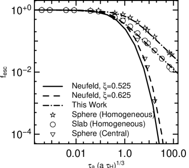
Figure 1: Escape fraction for Lyman-$\alpha$  photons emitted inside different dusty gas configurations as a function of the product $\tau_{a}(a\tau_{H})^{1/3}$. Symbols represent the results obtained with CLARA. The empty triangles show the solution for a dusty sphere when the photons are emitted at the centre of the sphere, whereas stars represent the case with Lyman-$\alpha$ sources homogeneously distributed in the sphere. Hexagons represent the results of the infinite dusty slab with sources homogeneously distributed. The solid line shows the analytical solution shown in Eq. (4) for the infinite dusty slab and sources located in the slab’s centre ($\xi=0.525$). The dashed and dotted line represent the same analytical expression with parameters $\xi=0.625$. A better fit for the homogeneous distributed sources (both for the sphere and the slab) is displayed by the dash-dotted line, see Eqs. (5) and (6).

The problem of an infinite homogeneous dusty gas slab has an analytic solution for the escape fraction provided that the sources are located in a thin plane. The dashed line in Figure 1 corresponds to the theoretical expectation (described in Appendix A, Eq.(34)) for the escape fraction out of a infinite slab as a function of the product $(a\tau_{0})^{1/3}\tau_{a}$,

$$f_{esc}=\frac{1}{\cosh\left(\xi^{\prime}\sqrt{(a\tau_{0})^{1/3}\tau_{a}}\right)},$$ (4)

where $\tau_{0}$ is the Hydrogen optical depth, $\tau_{a}$ is the optical depth of absorbing material (for albedo values of $A$, $\tau_{a}=(1-A)\tau_{d}$, where $\tau_{d}$ is the dust optical depth), and $a$ is a measure of the temperature in the gas defined as $a=\Delta\nu_{L}/(2\Delta\nu_{D})$, $\Delta\nu_{D}=(v_{p}/c)\nu_{0}$ is the Doppler frequency width, and $v_{p}=(2kT/m_{H})^{1/2}$ is $\sqrt{2}$ times the velocity dispersion of the Hydrogen atom, $T$ is the gas temperature, $m_{H}$ is the Hydrogen atom mass and $\Delta\nu_{L}$ is the natural line width. The constant $\xi^{\prime}=\xi\sqrt{3}/\pi^{5/12}$ and $\xi$ is a free parameter taking a value of $\xi=0.525$ in the case of centrally located sources.

For comparison, we show the results in the case of a homogeneous dusty gas sphere with centrally located sources of Lyman-$\alpha$ radiation. This configuration is fully parameterised by the optical depth of Hydrogen and dust as measured from the centre of the sphere to its boundary. We simulate with CLARA a series of spheres with different values for these optical depths (see Table 1). The empty triangles in Figure 1 represents the results for that configuration. The main point of this numerical experiment is to confirm that the same function that is used to describe the escape fraction of the infinite slab seems to be able to describe the escape fraction out of the sphere in the case of centrally located sources. The only difference is the value for the constant, in the spherical case $\xi=0.625$. Nevertheless, the differences between both geometries for the gas density and the dust abundance, at a given temperature, are never larger than a factor of 4, for the range of parameters studied.

We now turn to the case where the sources of Lyman-$\alpha$ radiation are homogeneously mixed inside the infinite slab. In this configuration we expect a higher escape fraction given the fact that the photons will be, on average, emitted closer to the escape surface. This will allow the photons to be affected by less collisions compared to the photons emitted at the centre of the slab. In Figure 1, the escape fraction for the homogeneous distribution of Lyman-$\alpha$ sources is shown by the hexagons. For small values of ${\mathcal{T}}\equiv\tau_{a}(a\tau_{0})^{1/3}$ the escape fraction seems to be well approximated by Eq.(4). For large values of $\mathcal{T}>1$ the escape fraction can be up to three orders of magnitude higher than in the central emission geometry in the range of explored values. The scaling of the escape fraction with the variable $\mathcal{T}$ does not follow Eq.(4). For large values of $\mathcal{T}>1$, the escape fraction shows a fall off almost proportional to $1/\mathcal{T}$. This can be understood in analogy to the classical case of continuum light emitted inside a dusty slab. As the optical depth reaches high values, only the photons emitted close to the surface within a distance $\propto 1/\tau$ have a high escape probability.

In analogy with the solution of continuum attenuation in a dusty slab, we find that for Lyman-$\alpha$ radiation, a solution with the functional form

$$f_{esc}=\frac{1-\exp(-P)}{P}$$ (5)

with

$$P=\epsilon((a\tau_{0})^{1/3}\tau_{a})^{3/4},$$ (6)

provides a reasonable description of the Monte-Carlo results as shown in Figure 1 (dot-dashed line) with $\epsilon=3.5$ in the slab geometry and $\epsilon=1.0$ in the spherical case.

We conclude that the source distribution, relative to the gas distribution, has a larger impact on the escape fraction than the geometrical distribution of the gas itself. The infinite slab exhibits very similar escape fraction compared to a spherical gas distribution, even the same scaling with respect to the gas properties holds. On the other hand, the homogeneous source distribution presents a radically different scaling with the optical depth in the gas, allowing for high escape fractions at large values of $(a\tau_{0})^{1/3}\tau_{a}>1$, both for the slab and spherical geometries. Additionally, the shape of the outgoing spectra, corrected for the escape fraction are different for the homogeneous vs. central source distribution (see Appendix A for the case of the dusty sphere).

4.2 Implementation in the MareNostrum Simulation

In the previous subsection, we obtained results on the escape fraction for the case of a homogeneous dusty gas slab with radiation sources distributed homogeneously. We provided a fitting formula (Eq. (5)) for the escape fraction as a function of the optical depths of gas and dust and the gas temperature. These results can be used by any galaxy evolution model that provides predictions for these quantities.

In our case, we use this formula to to derive the values of the escape fraction for each galaxy in the MareNostrum High-z Universe simulation. In what follows, we explain how we proceed to estimate the physical quantities we need: $\tau_{0}$, $\tau_{a}$ and $a$.

First, we recall from Section 3 that the dust model described above splits the extinction into two contributions:

1. the extinction by the homogeneous ISM on all stars in the galaxy,

2. the extinction by the birth clouds around young stars.

We now want to have estimates for the escape fraction associated with the homogeneous ISM, $f_{esc}^{ISM}$, and with the birth clouds, $f_{esc}^{BC}$.

In order to estimate the ISM escape fraction, $f_{esc}^{ISM}$ we describe the ISM as a slab of constant density and temperature of $10^{4}$K, which fixes the value of $a=4.7\times 10^{-4}$. The hydrogen column density of this slab is given by Eq.(2). The average optical depth of neutral hydrogen is calculated from this column density and the hydrogen cross section at the center of the Lyman alpha line at a temperature of $10^{4}$K. Based on the results of the previous subsection, we have thus determined all the parameters we need to calculate the escape fraction in the slab approximation: the optical depth of dust and Hydrogen ($\tau^{ISM}_{d}$, $\tau^{ISM}_{H}$) and the gas temperature $T$.

We now have to estimate the escape fraction associated with the birth clouds, $f_{esc}^{BC}$. As all the Lyman-$\alpha$ emission comes from these regions, the full intrinsic Lyman-$\alpha$ luminosity has to be corrected as well by this escape fraction. The dust optical depth associated with the clouds, $\tau_{d}^{BC}$, has already been calculated using Eq.(3). On the other hand, the optical depth of hydrogen in the birth clouds, $\tau^{BC}_{H}$, still has to be estimated. Based on observations of large molecular clouds, the neutral Hydrogen column density in the densest regions is of the order of $10^{19}$ cm^-2 (Wannier et al., 1983). This is already $\sim 3$ orders of magnitude lower than the optical depth in our simulated galaxies at high redshift. Moreover, the warm regions have densities two orders of magnitudes lower (Ferrière, 2001). A realistic estimate then puts the average neutral Hydrogen optical depth $\sim 10^{5}$ times lower than the one estimated for the full galaxy. Under these conditions, we find within the cloud $\tau^{BC}_{0}\sim\tau^{BC}_{d}$ with $a\tau^{BC}_{H}<1$ and $\tau^{BC}_{d}>1$, making the extinction enhancement by resonant scattering irrelevant. In this case, we can take the escape fraction as the continuum extinction at $\lambda=1260$Å for a spherical geometry.

4.3 Comparison against observational constraints

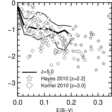
Figure 2: Escape fraction as a function of the UV color excess as estimated from the homogeneous ISM model. The lines show different distributions obtained from the simulation, the thick line marks the median, and the thin lines the first and third quartile. Stars represent observational estimates of the escape fraction at $z\sim 2.2$ by Hayes et al. (2010). Diamonds represent similar estimates at $z\sim 3.0$ by Kornei et al. (2010) In the left panel, the different lines show the evolution between $5<z<7$. We observe how to lower redshift values, higher values of the color excess are present. The very weak redshift evolution justifies the comparison of the results of this model against observations shown in the right panel. Only the simulated galaxies above the resolution threshold were taken into account in the calculation. The slab model with homogeneous source distribution matches closely the observed scaling of the escape fraction with colour excess.

Observational estimates of the escape fraction at redshifts $z\gtrsim 5$ (the lowest current redshift of the MareNostrum High-z Universe simulation) are not available. Nevertheless, at redshifts $z\sim 3$ the homogeneous ISM model is already consistent with the reddening scaling with galaxy luminosity (Shapley et al., 2001). It is then reasonable to think that at all redshifts $z<3$ the homogeneous ISM is still the appropriate model regarding the extinction. For this reason, we decide to compare the escape fraction predicted by the homogeneous ISM with the observational results at $z\sim 2.2$ and $z\sim 3$.

In the left panel of Figure 2 we present the redshift evolution of the escape fraction as a function of reddening at redshifts $z\sim 5$, $6$, $7$. We find that there is a weak redshift dependence. The biggest difference at each redshift is the presence of galaxies with larger values of colour excess. As the redshift evolution of the overall scaling is rather weak, we compare our theoretical results at $z\sim 5$, the last redshift available in the simulation to make this study, with the observations at $z\sim 2.2$ and $z\sim 3$, the highest redshifts so far with observations of this kind. The physical time between the observational results and the simulated ones is $\sim 1$Gyr.

In the right panel of Figure 2 we show the final result of the comparison between the escape fractions from observations at $z\sim 2.2$ and $z\sim 3$ and our model applied to the galaxies in the simulation at $z\sim 5$. The empty symbols represent the observational data, indeed showing a strong scaling: the escape fraction decreases with increasing colour excess. Our simple model of a dusty gas slab with homogeneously distributed sources reproduces well these observational trends determined by Hayes et al. (2010) and Kornei et al. (2010).

In order to facilitate the comparison of our results with those from other works (Kornei et al., 2010; Hayes et al., 2010), we also use the functional form $f_{esc}=C_{Ly\alpha}10^{-0.4\cdot E_{(B-V)}\cdot k_{Ly\alpha}}$ to fit the trend of the median values in the $f_{esc}$-$E(B-V)$ plane. This form takes into account that $C_{Ly\alpha}\neq 1$ for very low extinction values ($E(B-V)\approx 0$), as it is expected due to the resonance nature of the Lyman-$\alpha$  line. We obtain $C_{Ly\alpha}=0.21\pm 0.05$ and $k_{Ly\alpha}=8.6\pm 1.0$, which is somewhat flatter than the value of $k_{Ly\alpha}=12.0$ obtained by Calzetti et al. (2000) for Lyman-$\alpha$  wavelengths.

5 Analysis and Results

In this section we present our results on the escape fraction applying the slab model to the gas and dust contents calculated from the MareNostrum High-z Universe simulation. We first derive useful scalings of the escape fraction with the mass of the DM halo hosting the galaxy. We then apply the estimated escape fraction to obtain the luminosity function of LAEs at high redshift, $z\gtrsim 5$. Given that at these redshifts the extinction model includes a component associated to the birth clouds of the stars, we will add this component for the comparison with the luminosity functions at these redshifts.

5.1 Scaling with Halo Mass

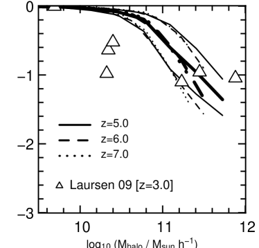
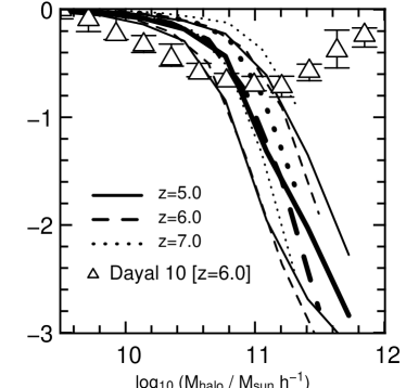
Figure 3: Escape fraction as a function of dark matter halo mass, for redshifts $z\sim 5$, $6$ and $7$. The thick lines mark the median, and the thin lines represent the first and third quartile. Triangles show different theoretical results. Left panel. The escape fraction includes the contribution from the homogeneous ISM ($f_{esc}^{ISM}$) only. The median values for $f_{esc}^{ISM}$ are reproduced by Eq. (7) The symbols correspond to the results for single halo simulations by Laursen et al. (2009). Right panel. Contribution from the birth clouds around the younger population stars to the escape fraction ($f_{esc}^{BC}$). The median values for $f_{esc}^{BC}$ are reproduced by Eq.(9). The symbols represent the results obtained by Dayal et al. (2010) from a cosmological simulation.

In the right panel of Figure 3 we show the total escape fraction $f_{esc}^{TOT}=f_{esc}^{ISM}\times f_{esc}^{BC}$ as a function of the host halo mass for the homogeneous slab model, where $f_{esc}^{ISM}$ and $f_{esc}^{BC}$ were defined in sub-section 4.2. The overall scaling of $f_{esc}^{ISM}$ and $f_{esc}^{BC}$ with halo mass follows the relation parameterized by Eq.(5) where the product $\tau_{a}(a\tau_{0})^{1/3}$ seems to be proportional to the halo mass.

Due to this shape, the escape fraction has a large scatter for galaxies in haloes more massive than $M_{c}=6\times 10^{10}{{h^{-1}{\rm{M_{\odot}}}}}$. The escape fraction for haloes less massive than this characteristic mass $M_{c}$ seems to be always larger than $10\%$.

We find that the median value of the escape fraction for the homogeneous $ISM$ component, $f_{esc}^{ISM}$, between redshifts $5\lesssim z\lesssim 7$ can be well approximated by the following expression:

$$f_{esc}^{ISM}=\frac{1-e^{-R}}{R},$$ (7)

where $R$ depends on the halo mass, $M_{h}$, as follows:

$$R=\left(\frac{M_{h}}{M_{c}}\right)^{5/3},$$ (8)

and the critical mass is equal to $M_{c}=6\times 10^{10}{{h^{-1}{\rm{M_{\odot}}}}}$.

Correspondingly, the median value of the escape fraction associated with the birth clouds of younger stellar populations, $f_{esc}^{BC}$, between redshifts $5\lesssim z\lesssim 7$ can be approximated by the following expression:

$$f_{esc}^{BC}=\frac{1-e^{-D}}{D},$$ (9)

where $D$ is equal to

$$D=\frac{1}{20}\left(\frac{1}{\mu}-1\right)\left(\frac{M_{h}}{M_{c}}\right)^{5/3}$$ (10)

and $M_{c}$ has the same value as in the case of the homogeneous ISM. The results in the last two equations are dependent on the dust abundances derived by matching the observed UV luminosity functions and the UV colours in the way presented in Forero-Romero et al. (2010).

The observed scatter in $f_{esc}^{TOT}$ can be reproduced in a Monte Carlo fashion if one calculates individual escape fractions $f_{esc}^{ISM}$ and $f_{esc}^{BC}$ from halo masses in the simulation, using Eqs. (7) and (9) with different values of $M_{c}$ and taking $\log_{10}M_{c}/{{h^{-1}{\rm{M_{\odot}}}}}$ as a Gaussian variable with mean $\log_{10}(6\times 10^{10})=10.77$ and variance of $0.3$.

In Figure 3 we compare our results against two other related theoretical works at high redshift. We start by pointing out that the observed scaling in our results follows closely the radiative transfer results shown in Figure 1. The correlation between halo mass and gaseous mass obtained in the simulation is translated here as a scaling between escape fraction and halo mass.

In the left panel of Figure 3 we compare our results of the escape fraction from the ISM component against the results of high resolution simulations of individual galaxies (Laursen et al., 2009). The two models show a good agreement for high and low halo masses. There is, however, a difference for haloes in the mass range $\sim 3\times 10^{10}$$h^{-1}{\rm{M_{\odot}}}$. The mean of our escape fractions is higher by a factor of $\sim 4$, although the small sample of Laursen et al. (2009) (seven galaxies) makes it difficult to estimate the statistical significance of this comparison between the two models.

In the right panel of Figure 3 we compare our results against a published model of the Lyman-$\alpha$ escape fraction in a cosmological context at $z\sim 6$ (Dayal et al., 2010). The model of Dayal et al. (2010) presents a radically different prediction for the escape fraction in haloes more massive than $M_{th}\sim 10^{11}$$h^{-1}{\rm{M_{\odot}}}$. While in our model the mean escape fraction drops steeply from $\sim 0.1$ down to $\sim 10^{-3}$, the results of Dayal et al. (2010) show an increase of the escape fraction to values close to $\sim 1$ for the same range of massive haloes. This disagreement is very likely due to the fact that Dayal et al. (2010) do not model explicitly the resonant nature of the line and approximate the ISM in such a way that the Lyman-$\alpha$  escape fraction is proportional to $(1-\exp-(\tau_{d}))/\tau_{d}$ where $\tau_{d}$ is the dust optical depth. This is a different approximation from the one that produces the results represented by Eq.5 and other similar radiative transfer studies (Hansen & Oh, 2006) where there is an explicit dependence with the optical depth of neutral gas, thought to be abundant in the most massive and vigorous star forming galaxies at these redshifts.

5.2 Intrinsic Emission and Luminosity Functions

We now study the LAE LF predicted from our simulations taking into account the different contributions to the escape fraction. We will focus on the intrinsic emission associated with star formation. The mechanism for star-triggered Lyman-$\alpha$  relates the amount of ionizing photons produced by young stars to the expected intrinsic Lyman-$\alpha$  luminosity. Here we assume that the number of Hydrogen ionizing photons per unit time is $1.8\times 10^{53}$ photons s^-1 for a star formation rate of $1$ ${\rm{M_{\odot}}}$/yr (Leitherer et al., 1999). This value assumes a Salpeter IMF, and that the star formation rate has been constant at least during the last $10$ Myr. Assuming that $2/3$ of these photons are converted to Lyman-$\alpha$ photons (case-B recombination, Osterbrock 1989), the intrinsic Lyman-$\alpha$ luminosity as a function of the star formation rate is

$$L_{Ly\alpha}=1.9\times 10^{42}\times({\mathrm{SFR}}/{\mathrm{M}}_{\odot}\ {\mathrm{yr}}^{-1}){\ \mathrm{erg\ s}}^{-1},$$ (11)

where the SFR is calculated from the total mass of stars produced in the last $200$ Myr. We use this analytic expression because the calculation of the total amount of ionizing photons directly from the information of the star particles in the simulation is not reliable given the short lifetime of the populations contributing to the ionizing flux and the limited resolution of our simulation. Only the star particles younger than $10$ Myr will provide the bulk of the ionizing flux, these particles roughly correspond to $1\%$ to $5\%$ of the star particles in a given galaxy. The least resolved galaxy in our study has $200$ star particles, which correspond to $2$ to $10$ particles to fully sample the star formation history of the galaxy during the last $10$ Myr. Only a handful of largest galaxies in the simulation ($\sim 100000$ star particles, $\sim 1000$ of them contributing to the ionizing flux) can give reliable results when the Lyman-$\alpha$ emission from the star particles is compared against Eq. (11).

We find a tight correlation between star formation rate and halo mass for $5\lesssim z\lesssim 7$. It can be approximated by

$${\mathrm{SFR}}=0.68\left(\frac{M_{h}}{10^{10}{{h^{-1}{\rm{M_{\odot}}}}}}\right)^{1.30}M_{\odot}\ {\mathrm{yr}}^{-1},$$ (12)

so that the final scaling between intrinsic Lyman-$\alpha$ emission and halo mass can be written as

$$L_{Ly\alpha}=1.29\times 10^{42}\left(\frac{M_{h}}{10^{10}{{h^{-1}{\rm{M_{\odot}}}}}}\right)^{1.30}{\mathrm{erg\ s}}^{-1}.$$ (13)

The observed Lyman-$\alpha$  luminosity can be calculated from our extinction model as:

$$L_{Ly\alpha}^{o}=(f^{ISM}_{esc}\times L_{Ly\alpha}^{old})+(f^{ISM}_{esc}\times f^{BC}_{esc}\times L_{Ly\alpha}^{young}),$$ (14)

where the label old refers to the Lyman-$\alpha$  emission coming from stellar populations older than $25$Myr and young labels the emission from stars younger than $25$ Myr. Given that the intrinsic ionizing flux is negligible for stellar populations older than $25$Myr, we can approximate the observed Lyman-$\alpha$  luminosity as:

$$L_{Ly\alpha}^{o}\approx f^{ISM}_{esc}\times f^{BC}_{esc}\times L_{Ly\alpha},$$ (15)

where the escape fractions $f^{ISM}_{esc}$ and $f^{BC}_{esc}$ are calculated as described in the previous subsections.

Previous Monte-Carlo calculations of Lyman-$\alpha$ radiative transfer in a multiphase medium (Hansen & Oh, 2006) show that the dominant effect of the clumpy distribution of birth clouds on a photon propagating through the homogeneous ISM is bouncing at the cloud’s surface, justifying the approximation of not including further absorption by these clouds except at the Lyman-$\alpha$ source in the way we have just implemented.

However, we note that the conditions for dust and gas abundance in our model are such that the calculations of Neufeld (1991) for the escape fraction are not applicable here. The main assumption of that model (negligible absorption and scattering in the homogeneous part of the ISM) are not met, meaning that the escape fraction in our model is not dominated by the effects of the clumpy component only.

We have not taken into account the effects of scattering of Lyman-$\alpha$ photons by the IGM, after they escaped from the galaxy. This effect is very important before reionisation ($z>6$ in our simulation). After reionisation, it is expected that the blue part of the double peak spectrum would be absorbed as photons are cosmologically redshifted to resonance with neutral Hydrogen along the line of sight. To first order, we have taken this effect into account by dividing the intensity of the observed line strength $L_{Ly\alpha}^{o}$ by $2$.

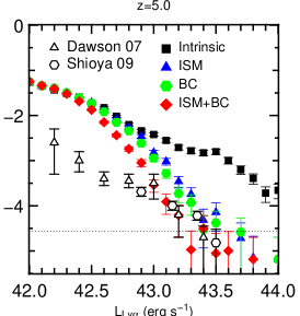
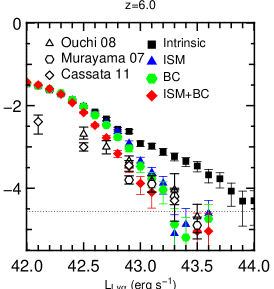
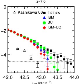
Figure 4: Luminosity Functions at $z\sim 5,6$ and $7$. The observational constraints (empty symbols) are compared to different results from the simulation (filled symbols): Intrinsic Lyman-$\alpha$ emission considering the total star formation rate in Eq.(11) (black squares), Lyman-$\alpha$ emission corrected only by the extinction of the homogeneous ISM based on the spherical model studied with the Monte Carlo simulations using Eq.(7) (blue triangles), Lyman-$\alpha$ emission corrected only by the extinction of the birth clouds using Eq.(9) (green hexagons). The final luminosity function corrected by the homogeneous ISM and the birth clouds is shown by the red diamonds.

In Figure 4 we show three different LAE LFs at three different redshifts $z\sim 5,6$ and $7$. The empty symbols represent the observed LFs. The observational results at $z\sim 4.5$ come from 50 spectroscopically confirmed LAEs from the Large Area Lyman-$\alpha$ survey (LALA) which covered a field of $\sim 0.7$ deg² corresponding to a comoving survey volume of $7.4\times 10^{5}$ Mpc³ (Dawson et al., 2007). At $z\sim 4.86$ the results from Shioya et al. (2009) are based on observations of the Cosmic Evolution Survey (COSMOS) field of $1.83$ deg² giving an effective volume of $1.1\times 10^{6}$ Mpc³. At $z\sim 6$ the data are taken from Ouchi et al. (2008), in this case the LF was estimated from LAEs from 1 deg² Subaru/XMM-Newton Deep Survey (SXDS), which probed a comoving volume of $\sim 10^{6}$ Mpc³. We include as well data at $z\sim 5.7$ in a field of $1.95$ deg² covered by the COSMOS survey Murayama et al. (2007) and recent estimations at $4.5<z<6.6$ from the Vimos-VLT Deep Survey (VVDS) (Cassata et al., 2011). The LF at $z\sim 7$ was constructed from a sample of 17 LAEs confirmed spectroscopically and 58 photometric LAEs probing a comoving volume of $\sim 2.17\times 10^{5}$ Mpc³ (Kashikawa et al., 2006). In our simulation we probe a comoving volume that is of the same order of magnitude of these surveys.

In Figure 4 we represent with black squares the LF estimated from the intrinsic luminosities calculated from the star formation rates. The spatial abundance is already corrected from the different halo abundance between the WMAP5 and the WMAP1 cosmologies. Compared with the observational estimates at all redshifts, the normalisation is at least one order of magnitude higher.

We can now apply the expected correction by the estimated escape fraction of each galaxy. In our model there is a strong correlation between the mass of the halo hosting the galaxy and its associated escape fraction. In a simplified manner, galaxies in haloes with masses smaller than $6.0\times 10^{10}$ $h^{-1}{\rm{M_{\odot}}}$remain practically unaffected. This is seen in the LFs in Figure 4 where the hexagons represent the luminosity function corrected by the escape fraction. The bright end of the LF is modified but the overall normalisation is kept one order of magnitude higher than observations.

This result is completely analogous to the situation found in the continuum UV using the same simulation (Forero-Romero et al., 2010). The strong scaling of the reddening with galaxy mass causes only the bright end of the UV LF to be effectively modified when extinction is taken into account. In the context of our model, applying a constant reddening value to all galaxies can only be physically justified if there is an additional extinction term from the youngest stars, as described in Section 3.

If we add now the expected correction of the birth clouds around stellar populations younger than $25$ Myr, we find that the faint end of the LAE LF can be further modified. However, at $z\sim 5$ and $z\sim 6$ there remains an excess at the faint end of the LF, corresponding to haloes with masses $1.0\times 10^{10}{{h^{-1}{\rm{M_{\odot}}}}}<M_{h}<4.0\times 10^{10}{{h^{-1}{\rm{M_{\odot}}}}}$. This result suggests that either the escape fraction for these galaxies or their star formation rate is too high. Nevertheless, the bright end of the simulated LFs, both at $z\sim 5$ and $z\sim 6$, shows a very close agreement with the observed one. The results are within Poissonian uncertainty. We have also checked that if we apply the scalings for the intrinsic emission and escape fractions with halo mass, Eqs. (7, 9, 13), to a pure DM only simulation with a cubic volume of $250$ $h^{-1}$Mpc on a side and $2048^{3}$ particles (the Bolshoi Simulation presented by Klypin et al. (2010)) split into smaller sub-boxes, we can reproduce the results we have just discussed. Specifically, the scatter at the bright end due to cosmic variance is consistent with the observations. Nevertheless, the same scatter does not help to explain the lower abundance of our numerical LAEs at the faint end.

The normalization of our LF functions at redshift $z\sim 7$ is still higher than observed. In principle, it could be possible to account for this difference by properly modeling the IGM absorption, which at this epoch, it is not completely ionized and will add a dimming effect to the LAEs. Considering a dimming factor that depends on luminosity only (without any scatter), we would require that 25% (40%) of Lya photons be transmitted through the IGM in order to match the bright (faint) end of the observed luminosity function. Using again the DM only simulation, together with the scalings we obtain for the star formation and the escape fraction, we find that cosmic variance can account for a 0.5 dex (0.3 dex) variations at the bright (faint) end of the luminosity function at $z\sim 7$. In conclusion, applying a constant IGM transmission of $T=0.3-0.4$ we can still reproduce the luminosity function for the brightest three bins in Figure 4. A more realistic treatment of the effects of IGM (in the spirit of Zheng et al. (2010)) actually yields a large scatter for the transmission at a given Lyman-$\alpha$  luminosity. Nevertheless, a detailed modeling of the IGM effect is far beyond the scope of this paper.

6 Conclusions

In this paper we model the escape fraction of Lyman-$\alpha$  photons in the approximation of a dusty gas slab with Lyman-$\alpha$  sources homogeneously mixed. The escape fractions for this configuration and different dust and gas contents have been calculated using CLARA, our new Monte-Carlo code described in detail in Appendix A. These results can be applied in any model that predicts the optical depth of gas and dust in galaxies.

We selected the slab geometrical configuration in order to be consistent with the assumptions that led us to fix the dust abundances from the MareNostrum High-z Universe simulation, as constrained by high redshift UV at $z\gtrsim 5$ observations (Forero-Romero et al., 2010). Our proposed dust model describes the contributions from an homogeneous ISM (slab geometry) and a clumpy phase (spherical geometry) associated to stellar populations younger than $25$Myr.

We estimate the scaling of the Lyman-$\alpha$  escape fraction with the expected reddening for the slab component and dust abundances in the MareNostrum High-z Universe. The scaling shows a weak redshift dependence between $5\lesssim z\lesssim 7$, furthermore there is a very good agreement with the observational estimation of the escape fraction and reddening for galaxies at $z\sim 2.2$ and $z\sim 3$ assuming that only the homogeneous ISM component is dominant at these redshifts. Including both contributions from the homogeneous ISM and the clumpy phase, we have calibrated the escape fraction as a function of the host dark matter halo based on the results of the MaraNostrum High-z Universe.

As an application of these results, we construct the intrinsic LAEs LF as estimated from the star formation rates. We find that the normalisation is one order of magnitude higher than observational estimates. Correcting the intrinsic LAE luminosities by the estimated escape fraction (homogeneous ISM and clumpy phase included) brings the simulation into agreement with the observations at $z\sim 5$ and $z\sim 6$. The match at the bright end is acceptable within the Poissonian and cosmic variance errors. The mismatch at $z\sim 7$ can be explained because a proper modeling of these epochs has to account for the yet incomplete reionisation process and the influence of the neutral parts of the IGM.

Nevertheless, our results are in conflict with the observational estimates at the faint end. There seems to be an excessive production of LAEs with intrinsic luminosities $L_{L\alpha}^{o}\sim 6.0\times 10^{42}$ erg s^-1 at $z\sim 5$ and $z\sim 6$. This excess was spotted, although weakly, in the results of the UV LFs of (Forero-Romero et al., 2010). Furthermore, a fine tuning of the extinction model for galaxies in this mass range could provide a better match to the observations. In that case, the galaxies at the faint end should be more dusty, which would make them redder, and thus breaking the broad agreement for the UV colours that we have already obtained. This is not a satisfactory approach to explain for these differences. Based on these considerations, we think that a probable origin of this discrepancy is the high rate of star formation in galaxies situated in these haloes. A possible physical explanation is that supernova feedback modulates more effectively the star formation in haloes of masses $<10^{11}$$h^{-1}{\rm{M_{\odot}}}$, providing a mechanism to shape the faint end of the luminosity function. However, it is also possible that the star formation rate is overestimated in all haloes at these redshifts. This would be translated into a trade-off with less dust extinction to explain the UV luminosity function. Regardless of what is the correct explanation of this enigma, all possible solutions seem to challenge our current understanding of the rate at which gas is converted into stars at high redshift.

It is encouraging that the results for the brightest galaxies, the best resolved ones, both in observations and simulations, are consistent with observations in the UV (magnitudes and colours) as well with the Lyman-$\alpha$ line. A full picture of these massive high redshift galaxies will be completed by observations of the rest frame IR to be performed by ALMA. We will address in a upcoming work the predictions of our model in terms of ALMA observations, focusing on the most massive galaxies, constructing a complete panchromatic perspective of high redshift galaxies in the MareNostrum High-z Universe.

Appendix A Lyman-$\alpha$ Radiative Transfer

The basic principle of CLARA is to follow the individual scatterings of a Lyman-$\alpha$ photon as it travels through a distribution of gaseous hydrogen. Each scattering, which is in fact an absorption and re-emission, does not modify the frequency of the photon in the rest-frame of the hydrogen atom. But due to the peculiar velocities of the atom in the new direction of propagation of the photon, the new frequency in a laboratory rest-frame is different from the incoming frequency. Thus the photon performs a random walk not only in space but also in frequency.

The relevant properties of the gaseous hydrogen can be fully described by its density, temperature and bulk velocity. This is sufficient to describe the emergent spectra of a source of Lyman-$\alpha$ photons embedded in gaseous hydrogen. It is important to observe that none of the emitted photons is completely lost by absorption as it is immediately re-emitted. The original spectrum morphology of the Lyman-$\alpha$ source is modified, but the only way to lose the energy input by a Lyman-$\alpha$ source is through dust absorption. A simple description of the dust abundance in the gas must then be included to calculate its effect on the outgoing properties of the traveling Lyman-$\alpha$ photons.

In the next subsections we give a detailed account on the basic underlying physics of the qualitative description we have just given. Once the physical fundamentals are described, we describe how these are implemented in the code. The last subsection is devoted to show the results available analytical test cases we applied the code to.

A.1 Physical Principles

A.1.1 Scattering

The scattering cross section of a Lyman-$\alpha$ photon is a function of the photon frequency. In the rest-frame of the atom it is equal to

$$\sigma(\nu)=f_{12}\frac{\pi e^{2}}{m_{e}c}\frac{\Delta\nu_{L}/2\pi}{(\nu-\nu_{0})^{2}+(\Delta\nu_{L}/2)^{2}},$$ (16)

where $f_{12}=0.4162$ is the Lyman-$\alpha$ oscillator strength, $\nu_{0}=2.466\times 10^{15}$Hz is the line centre frequency, $\Delta\nu_{L}=4.03\times 10^{-8}\nu_{0}=9.936\times 10^{7}$ Hz is the natural line width, and the others symbols conserve their usual meaning.

In the case of a Maxwellian distribution of atom velocities, after convolving the individual cross section with the atom velocity distribution, we can write down the average cross section as

$$\sigma(x)=\sigma_{x}=f_{12}\frac{\sqrt{\pi}e^{2}}{m_{e}c\Delta\nu_{D}}H(a,x),$$ (17)

where $H(a,x)$ is the Voigt function,

$$H(a,x)=\frac{a}{\pi}\int_{-\infty}^{\infty}\frac{e^{-y^{2}}}{(x-y)^{2}+a^{2}}dy,$$ (18)

$\Delta\nu_{D}=(v_{p}/c)\nu_{0}$ is the Doppler frequency width, $v_{p}=(2kT/m_{H})^{1/2}$ is $\sqrt{2}$ times the velocity dispersion of the Hydrogen atom, $T$ is the gas temperature, $m_{H}$ is the Hydrogen atom mass, $a=\Delta\nu_{L}/(2\Delta\nu_{D})$ is the relative line width and $x=(\nu_{i}-\nu_{0})/\Delta\nu_{D}$ is a re-parameterisation of the photon frequency respect to the line centre normalised by the temperature dependent Doppler frequency width of the gas.

The scattering is coherent in the rest-frame of the photon, but to an external observer, any motion of the atom will add a Doppler shift to the photon. Measuring the velocity of the atom, ${\bf v}_{a}$, in units of thermal velocity ${\bf u}={\bf v}_{a}/v_{p}$, the frequency in the reference frame of the atom is

$$x^{\prime}=x-{\bf u}\cdot{\bf n}_{i},$$ (19)

where ${\bf n}_{i}$ is a unit vector in the incoming direction of the photon.

In the general case, the scattering of the Lyman-$\alpha$ atom is not isotropic. For symmetry reasons the scattering is isotropic in the azimuthal direction, respect to the outgoing scattering direction. The distribution of the scatter directions depends only on the angle, $\theta$, between the incoming and outgoing direction of the photons, ${\bf n}_{i}$ and ${\bf n}_{o}$, respectively.

The information on the outgoing angle $\theta$ is encoded in the phase function, $W(\theta)$. In general the angular momenta of the initial, intermediate and final states are involved in the calculation of $W(\theta)$. In the case of resonant scatter the initial and final state are the same. The intermediate state corresponds to the excited state. Following the notation $nl_{J}$There are two possible excited states, $2P_{1/2}$ and $2P_{3/2}$.

Specifically, in the dipole approximation the phase function can be written as:

$$W(\theta)\propto 1+\frac{R}{Q}\cos^{2}\theta$$ (20)

where $R/Q=0$ for the $2P_{1/2}\to 1S_{1/2}$ transition and $R/Q=3/7$ for the $2P_{3/2}\to 1S_{1/2}$ case.

The spin multiplicity of each sate is $2J+1$, meaning that the probability of being excited to the $2P_{2/3}$ state is twice that of the $2P_{1/2}$ state. These results are valid only in the core of the line profile. Stenflo (1976) found that in the wings quantum mechanical interference between the two lines act in such a way as to give a scattering resembling a classical oscillator. In that case the phase function takes the form

$$W(\theta)\propto 1+\cos^{2}\theta$$ (21)

The travelling distance, $l$, of a Lyman-$\alpha$ photon of frequency $x$ can be expressed as

$$\tau_{x}=\sigma_{s}n_{H}l,$$ (22)

where $n_{H}$ is the neutral hydrogen number density, and it has been assumed that along the path $l$ the temperature and bulk velocity field of the gas are constant, to ensure that the photon frequency can be represented by the same value of $x$ along its trajectory.

In what follows, we will always characterise an homogeneous and static medium using the optical depth $\tau_{0}$ at the line center.

A.1.2 Dust Absorption

In the case of dust interaction the photon can either be scattered or absorbed. The optical depth of dust, $\sigma_{d}$, can be generally expressed as the sum of an absorption cross section $\sigma_{a}$, and a scattering cross section $\sigma_{s}$.

$$\sigma_{d}=\sigma_{a}+\sigma_{s}.$$ (23)

The determination of these two cross sections can be achieved using two different approaches. We name the first approach the ab initio approach. The ab initio approach seeks to determine the values of the dust cross sections from individual studies of dust grain properties and its interaction with photons. This is the approach used in the studies by Verhamme et al. (2006). The second approach is a phenomenological one and it defines the dust properties in relation to the gas properties in the galaxy. The dust cross section properties are then derived from observations. In the interest of keeping our model simple to operate and with a good match to the level of detail required for the approximation, we proceed with an ab initio approach.

We express then the absorption and scattering cross sections as

$$\sigma_{a,s}=\pi d^{2}Q_{a,s},$$ (24)

where $d$ is represents an average dust radius and $Q_{a,s}$ is an absorption/scattering efficiency. The dust albedo can be then expressed as

$$A=\frac{Q_{s}}{Q_{a}+Q_{s}}.$$ (25)

At UV wavelengths the emission and absorption processes are equally likely, with $Q_{a}\sim Q_{s}\sim 1$, making the dust albedo around $\sim 1/2$. We now express the dust of optical depth, $\tau_{d}$ in an analogous way to the neutral hydrogen optical depth Eq.(22) for a parcel of dust of linear dimensions $l$

$$\tau_{d}=\sigma_{d}n_{d}l,$$ (26)

where $n_{d}$ represents the number density of dust particles and it has been assumed again that the dust cross section and dust number density are constant on the scale of $l$.

A.2 The Radiative Transfer Code

The code implements a Monte Carlo approach to the radiative transfer. CLARA follows the successive scattering of individual photons as they travel through the gas distribution, changing at each scatter the direction of propagation and frequency of the photon. We describe now in detail the technical implementation.

A.2.1 Initial Conditions

The problem to solve defines the physical characteristics of the gas distribution and the initial conditions of the Lyman-$\alpha$ emitted photons. The gas is described by the following characteristics:

• The geometry of the gas distribution. In this section we will present results for the following configurations: infinite slab and sphere

• The size of the gas distribution. This is parameterised by the hydrogen optical depth, $\tau_{0}$ at line centre $x=0$. In all the geometries we measure the optical depth from the centre of the configuration to its nearest border.

• The temperature of the gas distribution, $T$. This is set to a constant for all the gas distributions explored in this paper.

• The gas bulk velocity field, ${\bf v_{b}}({\bf r})$. This is in general dependent on the position. The only bulk velocity field explored in this work corresponds to a Hubble like flow in the spherical geometries.

• The dust optical depth, $\tau_{d}$.

• The dust albedo, $A$.

The photons are described by the following properties:

• The spatial distribution with respect to the gas distribution. There are two possibilities. All the photons are emitted from the centre of the gas distribution or they are homogeneously distributed throughout the gas volume.

• The initial direction of propagation. We assume that the emission is isotropic (in the local comoving frame).

• The initial frequency, $x_{i}$. We consider that all photons are injected in the centre of the line $x_{i}=0$.

The number of photons used in order to reach convergence are $N_{ph}\sim 5\times 10^{4}$. In some cases convergence is reached with $N_{ph}\sim 1\times 10^{4}$ photons.

A.2.2 Photon Displacement and Interaction

For each photon of frequency $x$ and direction of propagation ${\bf n}_{i}$, we determine the distance freely travelled until the next interaction. This optical depth is determined by sampling the probability distribution $P(\tau)=\exp(-\tau)$ by setting $\tau_{s}=-\ln({{{\mathcal{R}}}})$, where ${\mathcal{R}}$ is a represents a random number between $0\leq{{{\mathcal{R}}}}<1$ following an uniform distribution.

This optical depth interaction fixes the travel distance $l_{s}$ by:

$$l_{s}=\frac{\tau_{s}}{\sigma_{x}n_{H}+\sigma_{d}n_{d}}$$ (27)

The photon travels a distance $l_{s}$ in the direction ${\bf b}_{i}$, at this point we decide if the photon interacts either with an hydrogen atom or with a dust grain. The probability of being scattered by a Hydrogen atom is

$$P_{H}=\frac{\sigma_{x}n_{H}}{\sigma_{x}n_{H}+\sigma_{d}n_{d}}.$$ (28)

Another random number ${{{\mathcal{R}}}}$ is generated and compared to $P_{H}$. If ${{{\mathcal{R}}}}<P_{H}$ the photon interacts with Hydrogen, otherwise it interacts with the dust grain. In the case of interaction with dust a new random number is generated and compared with the albedo $A$. If the random number is less than the albedo, the photon is scattered coherently in a random direction, otherwise the photon is absorbed and not considered for further scatterings during the rest of the simulation.

In the case of photon interaction, the situation is more involved. As already described by Eq. (19), the new photon frequency in the observer frame depends on the specific velocity of the atom, ${\bf u}$. It is therefore necessary to draw a velocity for the hydrogen atom. The preferred velocity for the atom cannot be drawn from a isotropic Gaussian distribution, there is an implicit spatial anisotropy in this case. The opacity of the gas is frequency dependent: the preferred atom velocity in the parallel direction to the photon propagation is different from the velocity in the perpendicular direction.

The atom velocity is thus determined in two steps. In the first step the two perpendicular velocities are selected from a Gaussian distribution. In the second step the parallel component of the atom velocity is calculated. The parallel component is calculated from a distribution calculated as the convolution of a Gaussian (representing the intrinsic velocity) convolved with the Lorentzian probability of the atom being able to scatter the photon:

$$f(u_{||})\propto{\mathcal{G}}(u_{||})\times{\mathcal{L}}(x-u_{||})\propto{e^{-u_{||}^{2}}}\times\frac{a}{\pi}\frac{1}{(x-u_{||})^{2}+a^{2}}.$$

The resulting normalised probability is:

$$f(u_{||})=\frac{a}{\pi H(a,x)}\frac{e^{u_{||}^{2}}}{(x-u_{||})^{2}+a^{2}}.$$ (29)

The distribution represented by Eq. (29) is not analytically integrable, therefore we generate the parallel velocities $u_{||}$ by means of the rejection method.

We stress that we do not use any of the commonly used speeding mechanisms. These speeding techniques are motivated by the physical fact that scattering of atoms in the core frequencies are irrelevant from the point of view of the change in frequency and position that they represent. Given the uncertainty of applying these techniques (despite of careful code calibration) in the presence of dust, we decide to use the simplest rejection method.

The new emission direction of propagation (in the atom rest-frame), ${\bf n}_{f}$ is determined as already described in detail in subsection A.1. In the observers frame, the final frequency is:

$$x_{f}=x_{i}-{\bf n}_{i}\cdot{\bf u}+{\bf n}_{f}\cdot{\bf u}+g(1-{\bf n}_{i}\cdot{\bf n}_{f}),$$ (30)

where the factor $g$ accounts for the recoil effect.

Figure 5: Analytical tests related to the infinite homogeneous gas slab. The left panel show the outgoing spectra for different hydrogen optical depths, compared to the expected analytical solutions. The middle panel compares the positions of the maxima in the outgoing spectra to the expected analytical estimates for a series of 5 different runs. The panel on the right compares the average number of scatterings the Lyman-$\alpha$ photons go through before escaping the slab. CLARA passes successfully these three tests.

A.3 Analytical Tests

$T(K)$	$\tau_{0}$	$V_{max}$	$\tau_{a}=(1-A)\tau_{d}$	$f_{esc,slab}^{C}$	$f_{esc,slab}^{H}$	$f_{esc,sph}^{C}$	$f_{esc,sph}^{H}$
$10^{4}$	$10^{6}$	0	$5.0\times 10^{-5}$	0.998	0.999	0.999	0.999
$10^{4}$	$10^{6}$	0	$5.0\times 10^{-4}$	0.991	0.993	0.995	0.997
$10^{4}$	$10^{6}$	0	$5.0\times 10{-3}$	0.917	0.937	0.957	0.976
$10^{4}$	$10^{6}$	0	$5.0\times 10^{-2}$	0.471	0.590	0.664	0.803
$10^{4}$	$10^{7}$	0	$5.0\times 10^{-5}$	0.998	0.998	0.999	0.999
$10^{4}$	$10^{7}$	0	$5.0\times 10^{-4}$	0.982	0.987	0.991	0.995
$10^{4}$	$10^{7}$	0	$5.0\times 10^{-3}$	0.853	0.894	0.925	0.962
$10^{4}$	$10^{7}$	0	$5.0\times 10^{-2}$	0.291	0.453	0.493	0.720
$10^{4}$	$10^{7}$	0	0.5	0.0029	0.084	0.014	0.224
$10^{4}$	$10^{7}$	0	0.1	0.127	0.295	0.280	0.568
$10^{4}$	$10^{7}$	0	0.2	0.036	0.179	0.111	0.407
$10^{4}$	$10^{7}$	0	0.4	0.0069	0.103	0.027	0.265
$10^{4}$	$10^{7}$	0	1.0	0.00023	0.049	0.0011	0.136
$10^{4}$	$10^{7}$	0	4.0	$<$ 0.0001	0.014	$<$0.0001	0.042
$10^{4}$	$10^{7}$	0	5.0	$<$ 0.0001	0.012	$<$0.0001	0.036
$10^{4}$	$1.2\times 10^{7}$	0	0.5	-	-	0.012	-
$10^{4}$	$1.2\times 10^{7}$	20	0.5	-	-	0.017	-
$10^{4}$	$1.2\times 10^{7}$	200	0.5	-	-	0.140	-
$10^{4}$	$1.2\times 10^{7}$	2000	0.5	-	-	0.283	-

Table 1: Summary of the physical characteristics for all runs, both with infinite slab and spherical geometry of a dusty gas distribution. $V_{max}$ refers to the parameterisation of the radial velocity profile imposed on the sphere following a Hubble-like law. The escape fraction in the case of centrally distributed sources in a sphere is denoted by $f_{esc,sph}^{C}$, while $f_{esc,sph}^{H}$ corresponds to the escape fraction when the Lyman-$\alpha$ sources are homogeneously distributed. The escape fractions for the infinite slab are denoted by $f_{esc,slab}^{C}$ and $f_{esc,slab}^{H}$.

The basic tests on CLARA are based on the available analytical solutions for a thick, plane-parallel, isothermal infinite gas slab of uniform density. The solution of the infinite slab provides the analytical expressions for: the distribution of outgoing frequencies, the average number of scatterings and the position of the peaks of the outgoing spectrum. In the case of a dusty infinite slab one we also have an analytical expression for the escape fraction (Harrington, 1973; Neufeld, 1991).

The expression for the analytic emergent spectrum as a function of frequency shift for a mid-plane source reads:

$$J(x)=\frac{\sqrt{6}}{24}\frac{1}{a\tau_{0}}\frac{x^{2}}{\cosh(\sqrt{\pi^{4}/54}|x^{3}-x_{i}^{3}|/a\tau_{0})},$$ (31)

where $\tau_{0}$ is the optical depth measured from the mid-plane to the slice boundary and $x_{i}$ is the frequency of the photons injected in the slice. For $x_{i}=0$ the emergent spectrum has a symmetric two-peaked shape.

Setting $\partial J/\partial x=0$ (Harrington, 1973), it can be shown that the position of the maxima is:

$$x_{m}=\pm 1.066(a\tau_{0})^{1/3},$$ (32)

while the average number of scatterings is:

$$\langle{N_{s}}\rangle=1.612\tau_{0}.$$ (33)

If dust is added to the gas distribution, it is then possible from analytical considerations to estimate the scalings of the escape fraction from the slab physical properties. The expression for the escape fraction reads

$$f_{esc}=\frac{1}{\cosh\left(\xi^{\prime}\sqrt{(a\tau_{0})^{1/3}\tau_{a}}\right)},$$ (34)

where $\xi^{\prime}=\xi\sqrt{3}/\pi^{5/12}$ and $\xi=0.565$ is a parameter found from a fit.

In the following we compare the analytical results described by Eqs.(31) to (34) with the results from CLARA . In Figure 5 we show the outgoing spectra for the infinite slab with four different optical depths $\tau_{0}=10^{5}$, $10^{6}$, $10^{7}$ and $10^{8}$, and a constant temperature of $T=10$K. The broad shape of the double peak is reproduced. The agreement with the expected analytical solution becomes better as the hydrogen optical depth increases, as expected. The simulation and the analytical result are expected to hold for optical depths and temperatures such as $a\tau_{0}>10^{3}$.

In the middle panel of Figure 5, we have the positions of the positive and negative peaks in the outgoing spectra, as a function of the product $a\tau_{0}$. These results were obtained from 7 different runs with their characteristics listed in Table 1. In the right panel we compare the number of scatterings with the theoretical prediction, which is only dependent on the hydrogen optical depth $\tau_{0}$. In both cases we find optimal agreement with the theoretical expectations. We stress again that even though we reproduce the right number of scatterings, we have not implemented any acceleration scheme based on the skip scattering scheme.

In Figure 6 we show the results concerning the escape fraction for the dusty infinite slab. We compare our results to the expected result from Eq. (34). In Table 1 we list the parameters for the dusty slab run, as well as the values of the escape fraction we find. The theoretical expectations for the escape fraction take the interaction with dust as an absorption. In the case of our runs, as we consider an albedo of $A=0.5$, the optical depth of dust grains has to be replaced by an effective value of an absorbing material $\tau_{a}=(1-A)\tau_{d}=0.5\tau_{d}$, where $\tau_{d}$ is defined by Eq. (26). Once again, we find a reasonable agreement with the theoretical expectations.

At this point we are confident that CLARA provides the expected outgoing spectra and number of scatterings. The dust implementation has been tested against the available theoretical constraints, yielding satisfactory results.

The case of spherical symmetry offers analytical solutions in specific cases (Dijkstra et al., 2006). Besides, the case of a expanding (contracting) sphere has been extensively studied in the literature with different Monte Carlo codes. The spherical symmetry situations gives us the possibility to perform further tests on CLARA. We will deal with the case of a static, isothermal and homogeneous sphere of gas first. Subsequently we will add a Hubble-like flow to the sphere.

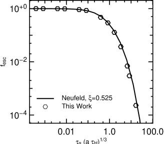
Figure 6: Escape fraction for Lyman-$\alpha$  photons emitted from the centre of a infinite slab of gas. The hexagons represent the results of CLARA, the continuous line, the analytical solution of Eq.(34).

Figure 7: Emergent line profile for the static and dustless sphere test. The photons are emitted at the centre of a sphere with different hydrogen optical depths. The analytical solution follows Dijkstra et al. (2006).

Figure 8: Emergent line profile in the collapsing/outflowing sphere tests. The collapsing/outflowing solutions are symmetric under parity transformations $x\leftrightarrow-x$.

Dijkstra et al. (2006) computed the analytic solution for the emergent spectrum of a point-like Lyman-$\alpha$ source surrounded by an homogeneous, static gas distribution at a constant temperature. The solution can be expressed with the same functional form as the Harrington-Neufeld solution (Harrington, 1973; Neufeld, 1991).

We setup different configurations in CLARA for a series of optical depth and temperatures. Figure 7 shows CLARA outputs compared with the corresponding analytical solutions. Once more, in the limit of large values for $a\tau_{0}>10^{3}$ we recover the behaviour expected by the analytical solution provided by Dijkstra et al. (2006).

We add to the homogeneous sphere a radial Hubble like flow as a function to the distance to the centre of the sphere

$$V_{r}(r)=V_{max}\frac{r}{R},$$ (35)

where $V_{max}$ is a constant which can be selected to be positive or negative.

The outgoing spectra of this type of configuration has not been worked out from an analytical point of view. However, it is part of the most studied physical setups by Monte Carlo codes similar to ours. The quantitative behaviour of our results follows the behaviour of previously published results. In the expanding case, there is suppression of the blue peak accompanied by an enhancement in the red wing of the emergent spectrum. The case of the collapsing sphere displays the enhancement in the blue peak and suppression in the red peak.

A.4 The Homogeneous Source Distribution

Figure 9: Emergent line profile in the case of a static dusty sphere. The parameters for the run where $T=10^{4}$K, $\tau_{0}=10^{7}$ and $\tau_{d}=0.4$. The profiles are corrected for the escape fraction. The different line profiles correspond to the case of centrally distributed sources versus homogeneously distributed. The case of centrally distributed sources is compatible with the analytic solution of Dijkstra et al. (2006). The case of homogeneously distributed sources presents a different line profile. The maxima are closer to the line center, and each peak is asymmetric respect to the maximum.

The model of the LAEs suggested in the paper is based on the approximation of an homogeneous dusty gas sphere, with the photon sources distributed homogeneously inside the sphere. In the body of the paper we explored in detail the consequences of this model on the escape fraction. At the same time we have studied the effect on the outgoing spectra.

Figure 9 presents the outgoing spectra already corrected by the escape fraction. The dashed line shows the result for the sphere with sources located at the center, the solid line is the expected result for the case of the dustless sphere. The match between the two curves shows that effectively the shape of the outgoing spectra is preserved in the presence of dust. This result is expected because all the photons are emitted at the same location and experience the same optical depth.

In case of homogeneously distributed sources, the spectral shape is different. The peaks are located closer to the line centre due to the fact that now, on average, the photons experience a smaller optical depth. At the same time, each wing presents now an asymmetrical shape with respect to these maxima. Furthermore, there is now some amount of photons very close to the center of the line, i.e. emitted close to the surface, that escaped without any scatter.

We have presented CLARA, a radiative transfer code for Lyman-$\alpha$ radiation. The code propagates Lyman-$\alpha$ photons through arbitrary distributions of hydrogen density, temperature, velocity structures and dust distributions. The code has successfully passed all the available tests for codes of its kind, and has allowed us to study simplified geometries in the present paper.

References

- Calzetti et al. (2000) Calzetti D., Armus L., Bohlin R. C., Kinney A. L., Koornneef J., Storchi-Bergmann T., 2000, ApJ, 533, 682
- Cassata et al. (2011) Cassata P., Le Fèvre O., Garilli B., Maccagni D., Le Brun V., Scodeggio M., Tresse L., Ilbert O. et al ., 2011, A&A, 525, A143+
- Cazaux & Spaans (2004) Cazaux S., Spaans M., 2004, ApJ, 611, 40
- Ceverino et al. (2010) Ceverino D., Dekel A., Bournaud F., 2010, MNRAS, 404, 2151
- Charlot & Fall (2000) Charlot S., Fall S. M., 2000, ApJ, 539, 718
- Dawson et al. (2007) Dawson S., Rhoads J. E., Malhotra S., Stern D., Wang J., Dey A., Spinrad H., Jannuzi B. T., 2007, ApJ, 671, 1227
- Dayal et al. (2010) Dayal P., Ferrara A., Saro A., 2010, MNRAS, 402, 1449
- Devriendt et al. (2010) Devriendt J., Rimes C., Pichon C., Teyssier R., Le Borgne D., Aubert D., Audit E., Colombi S., Courty S., Dubois Y., Prunet S., Rasera Y., Slyz A., Tweed D., 2010, MNRAS, 403, L84
- Devriendt et al. (1999) Devriendt J. E. G., Guiderdoni B., Sadat R., 1999, A&A, 350, 381
- Dijkstra et al. (2006) Dijkstra M., Haiman Z., Spaans M., 2006, ApJ, 649, 14
- Dunkley et al. (2009) Dunkley J., Komatsu E., Nolta M. R., Spergel D. N., Larson D., Hinshaw G., Page L., Bennett C. L., Gold B., Jarosik N., Weiland J. L., Halpern M., Hill R. S., Kogut A., Limon M., Meyer S. S., Tucker G. S., Wollack E., Wright E. L., 2009, ApJS, 180, 306
- Eisenstein et al. (2005) Eisenstein et al. 2005, ApJ, 633, 560
- Ferrière (2001) Ferrière K. M., 2001, Reviews of Modern Physics, 73, 1031
- Finlator et al. (2011) Finlator K., Oppenheimer B. D., Davé R., 2011, MNRAS, 410, 1703
- Forero-Romero et al. (2010) Forero-Romero J. E., Yepes G., Gottlöber S., Knollmann S. R., Khalatyan A., Cuesta A. J., Prada F., 2010, MNRAS, 403, L31
- Hansen & Oh (2006) Hansen M., Oh S. P., 2006, MNRAS, 367, 979
- Harrington (1973) Harrington J. P., 1973, MNRAS, 162, 43
- Hatton et al. (2003) Hatton S., Devriendt J. E. G., Ninin S., Bouchet F. R., Guiderdoni B., Vibert D., 2003, MNRAS, 343, 75
- Hayes et al. (2010) Hayes M., Östlin G., Schaerer D., Mas-Hesse J. M., Leitherer C., Atek H., Kunth D., Verhamme A., de Barros S., Melinder J., 2010, Nature, 464, 562
- Hill et al. (2008) Hill G. J., Gebhardt K., Komatsu E., Drory N., MacQueen P. J., Adams J., Blanc G. A., Koehler R., Rafal M., Roth M. M., Kelz A., Gronwall C., Ciardullo R., Schneider D. P., 2008, in T. Kodama, T. Yamada, & K. Aoki ed., Astronomical Society of the Pacific Conference Series Vol. 399 of Astronomical Society of the Pacific Conference Series, The Hobby-Eberly Telescope Dark Energy Experiment (HETDEX): Description and Early Pilot Survey Results. pp 115–+
- Hirashita et al. (2005) Hirashita H., Nozawa T., Kozasa T., Ishii T. T., Takeuchi T. T., 2005, MNRAS, 357, 1077
- Hu & McMahon (1996) Hu E., McMahon R. G., 1996, Nature, 382, 281
- Hu et al. (2005) Hu E. M., Cowie L. L., Capak P., Kakazu Y., 2005, in P. Williams, C.-G. Shu, & B. Menard ed., IAU Colloq. 199: Probing Galaxies through Quasar Absorption Lines Spectroscopic studies of and galaxies: implications for reionisation. pp 363–368
- Hu et al. (2004) Hu E. M., Cowie L. L., Capak P., McMahon R. G., Hayashino T., Komiyama Y., 2004, AJ, 127, 563
- Hu et al. (1998) Hu E. M., Cowie L. L., McMahon R. G., 1998, ApJL, 502, L99+
- Hu et al. (2002) Hu E. M., Cowie L. L., McMahon R. G., Capak P., Iwamuro F., Kneib J., Maihara T., Motohara K., 2002, ApJL, 568, L75
- Inoue (2003) Inoue A. K., 2003, PASJ, 55, 901
- Inoue (2005) Inoue A. K., 2005, MNRAS, 359, 171
- Kashikawa et al. (2006) Kashikawa N., Shimasaku K., Malkan M. A., Doi M., Matsuda Y., Ouchi M., Taniguchi Y., Ly C., Nagao T., Iye M., Motohara K., Murayama T., Murozono K., Nariai K., Ohta K., Okamura S., Sasaki T., Shioya Y., Umemura M., 2006, ApJ, 648, 7
- Klypin et al. (2010) Klypin A., Trujillo-Gomez S., Primack J., 2010, ArXiv e-prints
- Knollmann & Knebe (2009) Knollmann S. R., Knebe A., 2009, ApJS, 182, 608
- Kobayashi et al. (2007) Kobayashi M. A. R., Totani T., Nagashima M., 2007, ApJ, 670, 919
- Kong et al. (2004) Kong X., Charlot S., Brinchmann J., Fall S. M., 2004, MNRAS, 349, 769
- Kornei et al. (2010) Kornei K. A., Shapley A. E., Erb D. K., Steidel C. C., Reddy N. A., Pettini M., Bogosavljević M., 2010, ApJ, 711, 693
- Laursen et al. (2009) Laursen P., Sommer-Larsen J., Andersen A. C., 2009, ApJ, 704, 1640
- Le Delliou et al. (2005) Le Delliou M., Lacey C., Baugh C. M., Guiderdoni B., Bacon R., Courtois H., Sousbie T., Morris S. L., 2005, MNRAS, 357, L11
- Leitherer et al. (1999) Leitherer C., Schaerer D., Goldader J. D., González Delgado R. M., Robert C., Kune D. F., de Mello D. F., Devost D., Heckman T. M., 1999, ApJS, 123, 3
- Malhotra & Rhoads (2004) Malhotra S., Rhoads J. E., 2004, ApJL, 617, L5
- Mathis et al. (1983) Mathis J. S., Mezger P. G., Panagia N., 1983, A&A, 128, 212
- Murayama et al. (2007) Murayama T., Taniguchi Y., Scoville N. Z., Ajiki M., Sanders D. B., Mobasher B., Aussel H., Capak P., Koekemoer A., Shioya Y., Nagao T., Carilli C., Ellis R. S., Garilli B., Giavalisco M., 2007, ApJS, 172, 523
- Neufeld (1991) Neufeld D. A., 1991, ApJL, 370, L85
- Night et al. (2006) Night C., Nagamine K., Springel V., Hernquist L., 2006, MNRAS, 366, 705
- Nilsson et al. (2007) Nilsson K. K., Orsi A., Lacey C. G., Baugh C. M., Thommes E., 2007, A&A, 474, 385
- Osterbrock (1989) Osterbrock D. E., 1989, Astrophysics of gaseous nebulae and active galactic nuclei
- Ota et al. (2008) Ota K., Iye M., Kashikawa N., Shimasaku K., Kobayashi M., Totani T., Nagashima M., Morokuma T., Furusawa H., Hattori T., Matsuda Y., Hashimoto T., Ouchi M., 2008, ApJ, 677, 12
- Ouchi et al. (2009) Ouchi M., Mobasher B., Shimasaku K., Ferguson H. C., Fall S. M., Ono Y., Kashikawa N., Morokuma T., Nakajima K., Okamura S., Dickinson M., Giavalisco M., Ohta K., 2009, ApJ, 706, 1136
- Ouchi et al. (2008) Ouchi M., Shimasaku K., Akiyama M., Simpson C., Saito T., Ueda Y., Furusawa H., Sekiguchi K., Yamada T., Kodama T., Kashikawa N., Okamura S., Iye M., Takata T., Yoshida M., Yoshida M., 2008, ApJS, 176, 301
- Partridge & Peebles (1967) Partridge R. B., Peebles P. J. E., 1967, ApJ, 147, 868
- Reddy et al. (2006) Reddy N. A., Steidel C. C., Fadda D., Yan L., Pettini M., Shapley A. E., Erb D. K., Adelberger K. L., 2006, ApJ, 644, 792
- Rhoads et al. (2003) Rhoads J. E., Dey A., Malhotra S., Stern D., Spinrad H., Jannuzi B. T., Dawson S., Brown M. J. I., Landes E., 2003, AJ, 125, 1006
- Shapley et al. (2001) Shapley A. E., Steidel C. C., Adelberger K. L., Dickinson M., Giavalisco M., Pettini M., 2001, ApJ, 562, 95
- Shimasaku et al. (2006) Shimasaku K., Kashikawa N., Doi M., Ly C., Malkan M. A., Matsuda Y., Ouchi M., Hayashino T., Iye M., Motohara K., Murayama T., Nagao T., Ohta K., Okamura S., Sasaki T., Shioya Y., Taniguchi Y., 2006, PASJ, 58, 313
- Shioya et al. (2009) Shioya Y., Taniguchi Y., Sasaki S. S., Nagao T., Murayama T., Saito T., Ideue Y., Nakajima A., Matsuoka K., Trump J., Scoville N. Z., Sanders D. B., 2009, ApJ, 696, 546
- Spergel et al. (2003) Spergel D. N., Verde L., Peiris H. V., Komatsu E., Nolta M. R., Bennett C. L., Halpern M., Hinshaw G., Jarosik N., Kogut A., Limon M., Meyer S. S., Page L., Tucker G. S., Weiland J. L., Wollack E., Wright E. L., 2003, ApJS, 148, 175
- Springel (2005) Springel V., 2005, MNRAS, 364, 1105
- Stark et al. (2007) Stark D. P., Ellis R. S., Richard J., Kneib J., Smith G. P., Santos M. R., 2007, ApJ, 663, 10
- Stenflo (1976) Stenflo J. O., 1976, A&A, 46, 61
- Trenti et al. (2010) Trenti M., Smith B. D., Hallman E. J., Skillman S. W., Shull J. M., 2010, ApJ, 711, 1198
- Verhamme et al. (2006) Verhamme A., Schaerer D., Maselli A., 2006, A&A, 460, 397
- Wagner et al. (2008) Wagner C., Müller V., Steinmetz M., 2008, A&A, 487, 63
- Wang et al. (2004) Wang J. X., Rhoads J. E., Malhotra S., Dawson S., Stern D., Dey A., Heckman T. M., Norman C. A., Spinrad H., 2004, ApJL, 608, L21
- Wannier et al. (1983) Wannier P. G., Lichten S. M., Morris M., 1983, ApJ, 268, 727
- Zheng et al. (2010) Zheng Z., Cen R., Trac H., Miralda-Escudé J., 2010, ApJ, 716, 574