QoS Provisioning for Multimedia Transmission in Cognitive Radio Networks

Abstract - In cognitive radio (CR) networks, the perceived reduction of application layer quality of service (QoS), such as multimedia distortion, by secondary users may impede the success of CR technologies. Most previous work in CR networks ignores application layer QoS. In this paper we take an integrated design approach to jointly optimize multimedia intra refreshing rate, an application layer parameter, together with access strategy, and spectrum sensing for multimedia transmission in a CR system with time varying wireless channels. Primary network usage and channel gain are modeled as a finite state Markov process. With channel sensing and channel state information errors, the system state cannot be directly observed. We formulate the QoS optimization problem as a partially observable Markov decision process (POMDP). A low complexity dynamic programming framework is presented to obtain the optimal policy. Simulation results show the effectiveness of the proposed scheme.

Keywords - Cognitive radio networks, multimedia, wireless networks.

1 Introduction

Recent widespread acceptance of wireless applications has triggered a huge demand for radio spectrum. For many years radio spectrum has been assigned to licensed (primary) users. Most of the time, some frequency bands in the radio spectrum remain largely unoccupied by primary users. Spectrum usage measurements by the Federal Communications Commission (FCC) show that at any given time and location, most of the spectrum is actually idle. That is, the spectrum shortage results from the spectrum management policy instead of the actual physical scarcity of usable spectrum. Cognitive radio (CR), which has been introduced in [1], is considered as an enabling technology that allows unlicensed (secondary) users to operate in the licensed spectrum bands. This can help overcome the lack of available spectrum in wireless communications. CR is capable of sensing its surrounding environment and adapting its internal states by making corresponding changes in certain operating parameters [2, 3, 4, 5]. The FCC in the United States began to consider more flexible use of available spectrum. The NeXt Generation program of the Defense Advanced Research Project Agency also aims to redistribute allocated spectrum dynamically.

One important application of CR is spectrum overlay dynamic spectrum access (DSA), where secondary users operate in the licensed band while limiting interference with primary users. Spectrum opportunities are detected and used by secondary users in the time and frequency domain [6, 7, 8]. An optimal spectrum sensing strategy is proposed in [9] to maximize throughput. A separation principle is established in [10] to decouple the design of the sensing strategy from that of the spectrum sensor and the access strategy. The benefits of cooperation in CR are illustrated in [11] and [12] for two- and multi-user networks, respectively. A dynamic frequency hopping scheme is presented in [13] for IEEE 802.22 wireless regional area networks, which is an emerging standard based on CR technologies. In [14], the authors present a game theoretical dynamic spectrum sharing framework for analysis of network users’ behaviors, efficient dynamic distributed design, and optimality analysis. Other game theoretic DSA methods are presented in [15, 16]. The authors in [17] exploit channel availability in the time domain and demonstrate the throughput performance for a Bluetooth/WLAN system. Spectrum opportunity is also exploited in the time domain in [18] where the authors present an ad hoc secondary MAC protocol to facilitate DSA.

Although much work has been done in CR networks, most previous work considers maximizing the throughput of secondary users as one of the most important design criteria. As a consequence, other QoS measures for secondary users, such as distortion for multimedia applications, are mostly ignored in the literature. However, recent work in cross-layer design shows that maximizing throughput does not necessarily benefit QoS at the application layer for some multimedia applications, such as video [19, 20]. From a user’s point of view, QoS at the application layer is more important than that at other layers. Moreover, CR-based services for secondary users would have a strictly lower QoS than radio services that enjoy guaranteed spectrum access [21, 22]. Therefore, if the application layer QoS is not carefully considered in CR networks, the perceived reduction in QoS associated with CR may impede the success of CR technologies.

Multimedia applications such as video telephony, conferencing, and video surveillance are being targeted for wireless networks, including CR networks. Lossy video compression standards, such as MPEG-4 and H.264, exploit the spatial and temporal redundancy in video streams to reduce the required bandwidth to transmit video. Compressed video comprises of intra- and inter-coded frames. The intra refreshing rate is an important application layer parameter [23]. Adaptively adjusting the intra refreshing rate for online video encoding applications can improve error resilience to the time varying wireless channels available to secondary users in CR networks.

Cross-layer wireless multimedia transmission, where parameter optimization is considered jointly across OSI layers, has been well studied in the literature [24, 25, 26, 27, 28]. Recent work shows promising improvement to video QoS by considering resource management, adaptation, and protection strategies available at the physical, medium access control, and network/transport layers in conjunction with multimedia compression and streaming algorithms [29, 30, 31, 32, 33, 34, 35]. Various channel adaptive distortion driven cross-layer transmission strategies have been explored. The authors in [36] investigate a classification based system where the optimal cross-layer strategy for various video and channel conditions are computed offline thereby reducing the transmission-time complexity of the compression and transmission strategy. Within a rate-distortion framework, source coding, retransmission, and adaptive modulation parameters are jointly considered for video summary in [37]. The authors in [38] take a cross-layer approach to allocate power level, source coding rate, and channel coding rate delivering basic and enhanced QoS levels for distant and near receivers in a CDMA network.

Although there are some cross-layer design techniques for wireless multimedia transmission in the literature, little work investigates channel adaptive multimedia transmission over a cognitive radio network. In this paper, we take an integrated design approach to jointly optimize application layer QoS for multimedia transmission over cognitive radio networks. Based on the sensed channel condition, secondary users can adapt the intra refreshing rate at the application layer, in addition to the parameters at other layers. Some distinct features of the proposed scheme are as follows.

• For secondary users in CR networks, channel selection for spectrum sensing, access decision, and intra refreshing rate are determined concurrently to maximize the QoS at the application layer (i.e., minimize distortion for video applications).

• Physical layer channel state information (CSI) (channel gain) is used by secondary users to help make the optimal decision to maximize the application layer QoS.

• Primary network usage and channel gain are modeled as a finite state Markov process. With channel sensing and CSI errors, the state cannot be directly observed. Following the work in [10], we formulate the whole system as a partially observable Markov decision process (POMDP) [39]. We extend the scheme to jointly optimizing application layer QoS for multimedia transmission over cognitive radio networks.

• Using simulation examples, we show that application layer parameters have significant impact on the QoS perceived by secondary users in CR networks. We also show that application layer QoS can be improved significantly if the intra refreshing rate is adapted together with parameters at low layers, such as spectrum sensing. This study reveals a number of interesting observations and provides insights into the design and optimization of CR networks from a cross-layer perspective.

The rest of the paper is organized as follows. Section II describes the multimedia transmission over CR networks problem. Section III presents the proposed scheme. Some simulation results are given in Section IV. Finally, we conclude this study in Section V.

2 Multimedia Transmission over Cognitive Radio Networks

In this section, we describe the multimedia rate-distortion model used in this paper. We then present the system model for multimedia transmission over cognitive radio networks.

2.1 Rate-Distortion (R-D) Model for Multimedia Applications

Wireless channels have limited bandwidth and are error-prone. Highly efficient coding algorithms such as H.264 and MPEG-4 can compress video to reduce the required bandwidth for the video stream. Rate control is used in video coding to control the video encoder output bit rate based on various conditions to improve video quality [40]. For example, the main tasks of MPEG-4 object-based video coding are (1) to determine how many bits are assigned to each video object in the scene and (2) to adjust the quantization parameter to accurately achieve the target coding bit rate [41].

Highly compressed video data is vulnerable to packet losses where a single bit error may cause severe distortion [42, 43]. This vulnerability makes error resilience at the video encoder essential. Intra update, also called intra refreshing, of macroblocks (MBs) is one approach for video error resilience and protection [44]. An intra coded MB does not need information from previous frames which may have already been corrupted by channel errors. This makes intra coded MBs an effective way to mitigate error propagation. Alternatively, with inter-coded MBs, channel errors from previous frames may still propagate to the current frame along the motion compensation path [45].

Given a source-coding bit rate $R_{s}$ and intra refreshing rate, we need a model to estimate the corresponding source distortion $D_{s}$. The authors in [23] provide a closed form distortion model taking into account varying characteristics of the input video, the sophisticated data representation scheme of the coding algorithm, and the intra refreshing rate. Based on the statistical analysis of the error propagation, error concealment, and channel decoding, a theoretical framework is developed to estimate the channel distortion, $D_{c}$. Coupled with the R-D model for source coding and time varying wireless channels an adaptive mode selection is proposed for wireless video coding and transmission.

We will use the rate-distortion model described in [23] in our study. The R-D model facilitates adaptive intra-mode selection and joint source-channel rate control

The total end-to-end distortion comprises of $D_{s}$, the quantization distortion introduced by the lossy video encoder to meet a target bit rate, and $D_{c}$, the distortion resulting from channel errors. For DCT-based video coding, intra coding of a MB or a frame usually requires more bits than inter coding since inter coding removes the temporal redundancy between two neighboring frames. Let $\beta$ be the intra refreshing rate, the percentage of MBs coded with intra mode. Inter coding of MBs has much better R-D performance than intra mode. Decreasing the intra refreshing rate decreases the source distortion for a target bit rate. However inter coding relies on information in previous frames. Packet losses due to channel errors result in error propagation along the motion-compensation path until the next intra coded MB is received. Increasing the intra refreshing rate decreases the channel distortion. Thus we have a tradeoff between source and channel distortion when selecting the intra refreshing rate. We aim to find the optimal $\beta$ to minimize the total end-to-end distortion given the channel bandwidth and packet loss ratio.

The source distortion is given by

$$D_{s}(R_{s},\beta)=D_{s}(R_{s},0)+\beta(1-\eta+\eta\beta)[D_{s}(R_{s},1)-D_{s}(R_{s},0)],$$ (1)

where $R_{s}$ denotes the source coding rate, $\beta$ is the intra refreshing rate, and $\eta$ is a constant based on the video sequence. $D_{s}(R_{s},0)$ and $D_{s}(R_{s},1)$ denotes the time average all inter- and intra-mode selection for all frames over $K$ time slots.

$$D_{s}(R_{s},0)=\frac{1}{K}\sum_{k=1}^{K}\frac{1}{M_{k}}\sum_{m=1}^{M_{k}}D_{s}(Rs,0,m),$$ (2)

$$D_{s}(R_{s},1)=\frac{1}{K}\sum_{k=1}^{K}\frac{1}{M_{k}}\sum_{m=1}^{M_{k}}D_{s}(Rs,1,m),$$ (3)

where $M_{k}$ is the number of inter/intra frames in time slot $k$. The average channel distortion for each time slot is given by

$$D_{c}(p,\beta)=\left(\frac{a}{1-b+b\beta}\right)\left(\frac{p}{1-p}\right)E[F_{d}(m,m-1)],$$ (4)

where $p$ is the packet loss rate, $b$ is a constant describing motion randomness of the video scene, $a$ is the energy loss ratio of the encoder filter, and $E[F_{d}(m,m-1)]$ is the average value of the frame difference $F_{d}(m,m-1)$ over $K$ slots. We will use the same error concealment strategy and packet loss ratio derivation as described in [23].

The total average distortion is given by

$$D(R_{s},p,\beta)=D_{s}(R_{s},\beta)+D_{c}(p,\beta).$$ (5)

The optimum $\beta^{*}$ is then selected to minimize the total distortion.

$$\beta^{*}=\hbox{arg}\min_{\beta}D(R_{s},p,\beta).$$ (6)

2.2 System Model

Consider a spectrum that consists of $N$ channels, each with bandwidth $W(n)$, $1\leq n\leq N$. These $N$ channels are licensed to primary users. Time is divided into slots of equal length $T$. Slot $k$ refers to the discrete time period $[kT,(k+1)T]$.

When the slot is not in use by primary users, it will be comprised of AWGN noise and fading. The fading process and primary usage for a channel can be represented by a stationary and ergodic $S$-state Markov chain. Let $i$ and $\gamma$ denote the instantaneous channel state and fading gain, respectively. When the channel is in state $i$, the quantized fading gain is $\gamma_{i}$, where $\gamma_{i}\leq\gamma\leq\gamma_{i+1}$, $1\leq i\leq S-1$. When the channel is in state $i=S$, the channel is in use by the primary network. We assume that the phase of the channel attenuation can be perfectly estimated and removed at the receiver. The $S$-state Markov channel model is completely described by its stationary distribution of each channel state $i$, denoted by $p(i)$, and the probability of transitioning from state $i$ into state $j$ after each time slot, denoted by $\{P_{i,j}\}$, $1\leq i,j\leq S$.

In general, a finite state Markov channel (FSMC) model is constructed for a particular fading distribution by first partitioning the range of the fading gain into a finite number of sections. Then each section of the gain value corresponds to a state in the Markov chain. The application of FSMC to model Rayleigh channels has been well studied in [46, 47]. Given knowledge of the fading process and primary network usage, the stationary distribution $p(i)$ as well as channel state transition probabilities $\{P_{i,j}\}$ can be derived. Once a channel gain has been determined for states 1,2,…, $S$-1, the packet loss ratio is determined for each state based on the modulation and channel coding schemes. The intra refreshing rate that minimizes the total distortion for each state can then be calculated using the Rate-Distortion model.

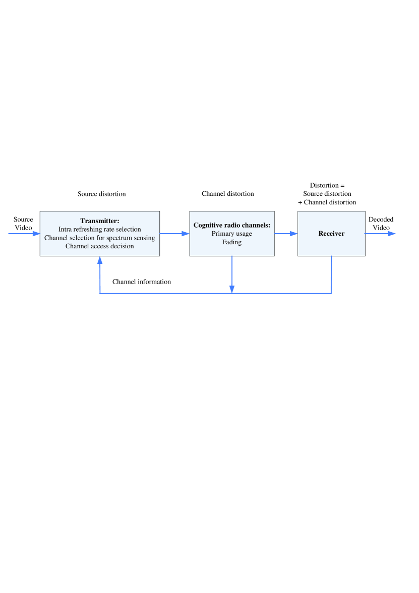
Figure 1: The Block diagram of multimedia transmission over cognitive radio networks.

At the beginning of a slot, the transmitter of secondary users will select a set of channels to sense. Based on the sensing outcome, the transmitter will decide whether or not to access a channel. If the transmitter decides to access a channel, some application layer parameters will be selected and the video content will be transmitted. At the end of the slot, the receiver will acknowledge the transfer by sending the perceived channel gain back to the transmitter. We will assume a system for real-time multimedia applications where packets are discarded if a primary user is using the slot or if the channel is not accessed. The system block diagram showing video transmission between two secondary users is shown in Fig. 1.

3 Solving the Multimedia Transmission over Cognitive Radio Networks Problem

In CR networks with multimedia applications, we need to determine the optimal policy for channel sensing selection, sensor operating point, access decision, and intra refreshing rate to minimize application layer distortion subject to the system probability of collision. With channel sensing and CSI errors, the system state cannot be directly observed. Following the work in [10], we formulate the whole system as a partially observable Markov decision process (POMDP). Deriving a single POMDP formulation for all policies under the probability of collision constraint would result in a constrained POMDP. However, constrained POMDPs require randomized policies to achieve optimality, which is often intractable. Therefore, we use the separation principle in [10] for the sensor operating point and the access decision. The spectrum sensor operating point is set such that $\delta=\zeta$, where $\delta$ is the probability of miss detection of the busy channel used by primary users and $\zeta$ is the required probability of collision.

At the beginning of the slot, the system transitions to a new state. Using a POMDP derived policy, a channel is selected for spectrum sensing. An access decision is then made based on the sensing observation. Using the belief of the channel state, an intra refreshing rate is selected. The receiver acknowledges the transfer by sending the quantized perceived channel gain back to the secondary transmitter. The immediate cost for the time slot is derived based on the previous operations in the slot.

The system can be formulated as a POMDP with states, actions, transition probabilities, observations, and cost structures as follows.

3.1 State Space, Transition Probabilities and Observation Space

The system state is given by the network usage of primary users and channel state information. Let $\{X(n)\}$ denote an $S$-state Markov chain for channel $n$, $X(n)\in\mathbb{X}=\{e_{1},e_{2},...,e_{S-1},e_{S}\}$, where $e_{i}$ denotes the $S$-dimensional unit vector with 1 in the $i$th position and zeros elsewhere. The system with $N$ channels is modeled as a discrete-time homogeneous Markov process with $S^{N}$ states. The system state in time slot $k$ is given by $V_{k}=[X_{k}(1),...,X_{k}(N)]$.

To simplify the presentation, we consider a system with a single channel in the formulation. It is straightforward to extend the formulation to include multiple channels which is considered in our simulations. For the system with a single channel, $V_{k}=X_{k}$. The transition probabilities of the system state are given by the $S\times S$ matrix $A$. We assume the transition probabilities are known based on network usage and channel fading characteristics.

The observation available to the secondary transmitter and receiver is the sensed channel and channel gain acknowledgment, $Y_{k}\in\mathbb{Y}$, where $\mathbb{Y}=\{{\gamma}_{1},...,{\gamma}_{S-1},{\gamma}_{S}\mbox{ (The channel is used by primary users)}\}$ and ${\gamma}_{i}<{\gamma}_{j},\forall i<j$.

The spectrum sensor observation may be different at the transmitter and receiver. If the transmitter and receiver use the same observations to derive the information state (described in the following Subsection), then the information state can be used to maintain frequency hopping synchronization. Thus the information state will be updated with $Y_{k}$ and will not include the spectrum sensor observation.

Let $B(y,x,a)=\mbox{Pr}\{y|x,a\}$ denote the conditional probability of observing $y$ given that the system state is in state $x$ and composite action $a$ was taken.

$$B(y,x,a)=\left\{\begin{array}[]{ll}P_{ce}(x,v(y))(1-\epsilon),&\mbox{if }y\neq{\gamma}_{S},x\neq e_{S},\\ \epsilon,&\mbox{if }y={\gamma}_{S},x\neq e_{S}\\ 0,&\mbox{if }y\neq{\gamma}_{S},x=e_{S}\\ 1,&\mbox{if }y={\gamma}_{S},x=e_{S}\end{array},\right.$$ (7)

where $\epsilon$ is the probability of miss detection of the idle channel and $v(y)=i$, $1<i<S$ given $y={\gamma}_{i}$. When the channel is available and accessed, the probability of channel estimate by the receiver is given by $P_{ce}(x,v(y))$ .

Using the work from Hoang and Motani [48], we assume the channel estimation error has a Gaussian distribution with zero mean and $\sigma^{2}$ variance. At a particular time and channel, the estimated channel gain is

$$\hat{\gamma}=\gamma_{i}+w,$$ (8)

where $\gamma_{i}$ is the actual channel gain and $w$ is a Gaussian random variable with zero mean and $\sigma^{2}$ variance. The receiver then quantizes the channel gain to the nearest possible value. The probability that $\hat{\gamma}$ is closest to $\gamma_{j}$ is given by

$$P_{ce}(i,j)=\left\{\begin{array}[]{ll}\frac{1}{2}\left[\mbox{erf}\left(\frac{\gamma_{j}+\gamma_{j+1}-2\gamma_{i}}{2\sqrt{2}\sigma}\right)-\mbox{erf}\left(\frac{\gamma_{j}+\gamma_{j-1}-2\gamma_{i}}{2\sqrt{2}\sigma}\right)\right],&\mbox{if }j\neq e_{1},e_{S-1},e_{S}\\ \frac{1}{2}\left[1+\mbox{erf}\left(\frac{\gamma_{1}+\gamma_{2}-2\gamma_{i}}{2\sqrt{2}\sigma}\right)\right],&\mbox{if }j=e_{1}\\ \frac{1}{2}\left[1-\mbox{erf}\left(\frac{\gamma_{S-2}+\gamma_{S-1}-2\gamma_{i}}{2\sqrt{2}\sigma}\right)\right],&\mbox{if }j=e_{S-1}\\ 0,&\mbox{if }j=e_{S}\end{array},\right.$$ (9)

where $\mbox{erf}()$ denotes the error function.

3.2 Information State

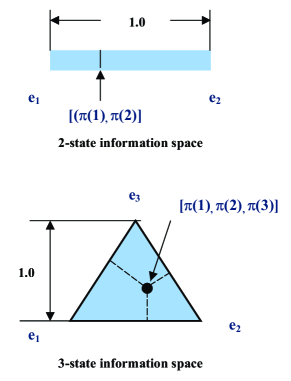
Figure 2: Information state in POMDP.

Information state is an important concept in POMDP. We will refer to a probability distribution over states as the information state and the entire probability space (the set of all possible probability distributions) as the information space. The information spaces for 2-state and 3-state systems are shown in Fig. 2. For a system with two states, its information space is a one-dimension line. The distance from the right end is the first component $\pi(1)$ and the distance from the left end is the second component $\pi(2)$. For the system with 3 states, its information space is a two-dimension triangle. The value of a point in the information space can be obtained from the perpendicular distance from the sides of the triangle. An information state is a sufficient statistic for the decision and observation history.

3.3 Action Space

Due to hardware limitations, we will assume that a secondary user is equipped with a single Neyman-Pearson energy detector and can only sense $L=1$ channel at each time instant. In each slot $k$, the secondary user needs to decide whether or not to sense, determine which sensor operating point on the Receiver Operating Curve (ROC) curve to use, whether to access the channel, and which quantized intra refreshing rate to use. Thus the action space consists of four parts: a channel selection decision $a_{s}(k)\in\{0(\mbox{no sense}),1(\mbox{sense})\}$, a spectrum sensor design $(\epsilon(k),\delta(k))\in\mathbb{A}_{\epsilon\delta}$ where $\mathbb{A}_{\epsilon\delta}$ are valid points on the ROC curve, an access decision $a_{a}(k)\in\{0(\mbox{no access}),1(\mbox{access})\}$, and an intra refreshing rate $\beta(k)\in\mathbb{A}_{\beta}$. The composite action in slot $k$ is denoted by $a_{k}=\{a_{s}(k),(\epsilon(k),\delta(k)),a_{a}(k),\beta(k)\}\in(\{0,1\},\mathbb{A}_{\epsilon\delta},\{0,1\},\mathbb{A}_{\beta})$.

Due to sensing and channel estimation errors, a secondary user cannot directly observe the true system state. It can infer the system state from its decision and observation history encapsulated by the information state. Information state $\pi_{k}=\{\lambda_{x}(k)\}_{x\in\mathbb{X}}\in\Pi(\mathbb{X})$ where $\lambda_{x}(k)\in[0,1]$ denotes the conditional probability (given decision and observation history) that the system state is in $x\in\mathbb{X}$ at the beginning of slot $k$ prior to state transition. $\Pi(\mathbb{X})=\{\lambda_{x}(k)\in[0,1],\sum_{x\in\mathbb{X}}\lambda_{x}=1\}$ denotes the information space that includes all possible probability mass functions on the state space $\mathbb{X}$.

At the end of the time slot, the transmitter receives observation $Y_{k}$. The information state is then updated using Bayes’ rule before state transition

$$\lambda_{k+1}=\frac{\sum_{x^{\prime}\in\mathbb{X}}\lambda_{x^{\prime}}(k)A_{x^{\prime},x}B(y_{k},x_{k},a_{k})}{\sum_{x\in\mathbb{X}}\sum_{x^{\prime}\in\mathbb{X}}\lambda_{x^{\prime}}(k)A_{x^{\prime},x}B(y_{k},x_{k},a_{k})}.$$ (10)

Given information vector $\pi_{k}$ the distribution of the system state $X_{k}$ in slot $k$ after state transition is then given by

$$\mbox{Pr}\{X_{k}=x\}=\sum_{x^{\prime}\in\mathbb{X}}\lambda_{x^{\prime}}(k)A_{x^{\prime},x}\;\forall x\in\mathbb{X}.$$ (11)

3.4 Cost and Policy

From a user’s point of view, QoS at application layer is more important than at other layers. Therefore, we model multimedia distortion as the immediate cost in our scheme. The immediate cost in time slot $k$ is defined as

$$C_{k}=D(R,p(x_{k},a_{k}),\beta(k)),$$ (12)

where $R$ is the target bit rate and $p(x_{k},a_{k})$ denotes the packet loss ratio when the system is in state $x_{k}$ and composite action $a_{k}$ is taken in time slot $k$. We assume $a_{a}(k)=0(\hbox{no access})$ is the equivalent to 100% packet loss.

The expected total cost of the POMDP represents the overall distortion for a video sequence transmitted over $K$ slots and can be expressed as

$$J_{\mu}=\mathbb{E}_{\{\mu_{s},\mu_{\epsilon\delta},\mu_{a},\mu_{\beta}\}}\left[\sum_{k=1}^{K}D(R,p(x_{k},a_{k}),\beta(k))\right],$$ (13)

where $\mathbb{E}_{\{\mu_{s},\mu_{\epsilon\delta},\mu_{a},\mu_{\beta}\}}$ indicates the expectation given that policies $\mu_{s},\mu_{\epsilon\delta},\mu_{a},\mu_{\beta}$ are employed.

A channel sensing policy $\mu_{s}$ specifies a channel to sense, $a_{s}$. A sensor operating policy $\mu_{\epsilon\delta}$ specifies a spectrum sensor design $(\epsilon,\delta)\in\mathbb{A}_{\epsilon\delta}$ based on the system tolerable probability of collision, $\zeta$. An access policy $\mu_{a}$ specifies the access decision $a_{a}\in\{0,1\}$. An intra refreshing policy $\mu_{\beta}$ specifies the intra refreshing decision ${\beta}\in\mathbb{A}_{\beta}$ based on the current information state $\pi_{k}$.

3.5 Objective and Constraint

We aim to develop the joint design of an optimal policy for multimedia transmission over CR networks, $\{\mu_{s}^{*},\mu_{\epsilon\delta}^{*},\mu_{a}^{*},\mu_{\beta}^{*}\}$, that minimizes the expected total distortion in $K$ slots under the collision constraint $P_{c}$.

$$\{\mu_{s}^{*},\mu_{\epsilon\delta}^{*},\mu_{a}^{*},\mu_{\beta}^{*}\} = \hbox{arg}\min_{\mu_{s},\mu_{\epsilon\delta},\mu_{a},\mu_{\beta}}\mathbb{E}_{\{\mu_{s},\mu_{\epsilon\delta},\mu_{a},\mu_{\beta}\}}\left[\sum_{k=1}^{K}D(R,p(x_{k},a_{k}),\beta(k))\right]$$ (14)

subject to

$$P_{c}(k) = \hbox{Pr}\{a_{a}(k)=1|X_{k}=e_{S}\}<\zeta\;,\forall k\in K.$$ (15)

3.6 Value Function

Let $J_{k}(\pi)$ be the value function that represents the minimum expected cost that can be obtained starting from slot $k$ $(1\leq k\leq K)$ given information state $\pi_{k}$ at the beginning of slot $k$. Given that the secondary user takes action $a_{k}$ and observes acknowledgment $Y_{k}=y_{k}$, the cost that can be accumulated starting from slot $k$ consists of the immediate cost $C_{k}=D(R,p(x_{k},a_{k}),\beta(k))$ and the minimum expected future cost $J_{k+1}(\pi+1)$. $\pi_{k+1}=\{\lambda_{x}(k+1)\}_{x\in\mathbb{X}}=U(\pi_{k}|a_{k},y_{k})$, which represents the updated knowledge of system state after incorporating the action $a_{k}$ and the acknowledgment $y_{k}$ in slot $k$. The sensing policy is then given by

$$J_{k}(\pi_{k}) = \min_{a\in\mathbb{A}}\sum_{x\in\mathbb{X}}\sum_{x^{\prime}\in\mathbb{X}}\lambda_{x^{\prime}}(k)A_{x^{\prime},x}\sum_{j=e_{1}}^{e_{S}}B(y_{k},j,a_{k})[D(R,p(x_{k},a_{k}),\beta(k))$$ (16)

$$+J_{k+1}(U(\pi_{k}|a_{k},y_{k}))],1\leq k\leq K-1$$

$$J_{K}(\pi_{K}) = \min_{a\in\mathbb{A}}\sum_{x\in\mathbb{X}}\sum_{x^{\prime}\in\mathbb{X}}\lambda_{x^{\prime}}(K)A_{x^{\prime},x}\left[\sum_{j=e_{1}}^{e_{S}}B(y_{K},j,a_{K})D(R,p(x_{K},a_{K}),\beta(K))\right].$$ (17)

The value function of an unconstrained POMDP with finite action space is piecewise-linear convex and can be solved using linear programming techniques [49]. An excellent overview of computationally efficient algorithms are given in [39] and can be used to solve for the optimum sensing policy. In general, the number of linear segments that characterize the value function can grow exponentially. In 1991, Lovejoy proposed an ingenious suboptimal algorithm for POMDPs [50]. Based on Lovejoy’s algorithm, the value function can be upper and lower bounded and efficient suboptimal solutions can be developed as in Subsection V-D of [51]. By considering only a subset of the piecewise linear segments that characterize the value function and discarding the other segments, one can reduce the computational complexity. Due to the space limitation, please refer to Subsection V-D of [51] for details. Moreover, solving the POMDP can be done off-line during system initialization. During the real-time multimedia transmission, a node just needs to find the value for specific information state according to (16) and update the information state according to (10), which introduces little computational complexity. Finally, by imposing structural assumptions on the transition probabilities, cost and observation probabilities, one can prove in some cases that the optimal policy is a threshold policy [52].

3.7 Intra Refreshing Strategy

For a selected channel, the optimum $\beta$ selected corresponds to the most likely available state based on $\pi_{k}$. Due to the asymptotic nature of the channel distortion, a busy or unaccessed channel has infinite distortion. In this case, $\beta$ has no influence on the total distortion. If the most likely state based on $\pi_{k}$ corresponds to a busy state then the optimum $\beta$ is to select a $\beta$ corresponding to the most likely available state. That way if the information state suggests the channel is busy but in reality it is available then a $\beta$ has been selected that will minimize the effect of this error.

4 Simulation Results and Discussions

In order to evaluate the performance of our proposed scheme, we have carried out a set of simulation experiments using the ns-2 simulator. All simulations were run on a computer equipped with Window 7, Intel Core 2 Duo P8400 CPU (2.26 Ghz) and 4GB memory. The choice for the total time slot number $K$ in the dynamic programming depends on the convergence rate of the POMDP program. State transition probabilities, observation probabilities and value functions have effects on the convergence rate [39], [49]. In our simulations, the POMDP program was run over a horizon of $K=200$. It is reasonable to use $K=200$ to approximate the problem with infinite horizon. We first consider a system with one channel in Subsections 4.1 - 4.3. Then, we consider a system with two channels in Subsections 4.4 - 4.5. In all figures the curves represent the average values, while the error bars represent the confidence intervals for 95 percent confidence for 50 different instances (seeds).

We consider the system performance in the following four cases: (1) using perfect knowledge of the system thus making optimal decisions, which is the best case possible, (2) making decisions based on the most likely state indicated by the information state, which is our proposed scheme, (3) making decisions solely based on the channel gain provided in the last acknowledgment, and (4) using a constant $\beta$, which represents existing schemes that do not consider application layer QoS. Our goal is to compare the distortion of different schemes as opposed to determining the absolute distortion. We use an average distortion metric that refers to the average distortion over the time slots when the channel is available and accessed. Video rate-distortion parameters remain constant for the duration of the simulation. The same distortion parameters are used for all simulations. $D_{s}(R_{s},0)=74$. $D_{s}(R_{s},1)=124$. $\eta=1.4$. $a=0.01$. $b=1.0$. $E[F_{d}(m,m-1)]=100$.

4.1 Performance Improvement

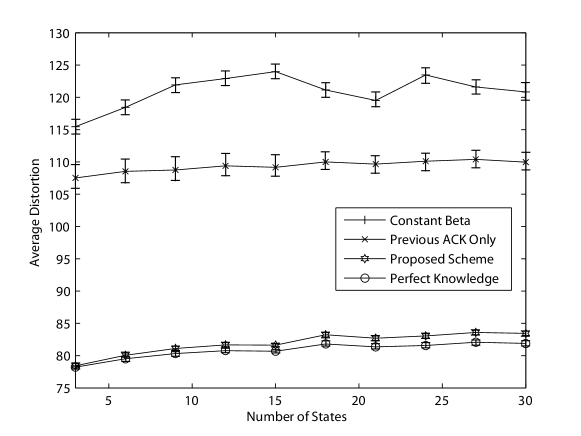
Figure 3: Average distortion vs. the number of states in different schemes.

Fig. 3 shows the distortion of different schemes. The number of states refers to $S-1$ quantized channel gains and one busy channel state. For simplicity we derive a transition matrix based on the probability that any available state stays in the same state, $\mbox{Pr}\{X_{k+1}=v|X_{k}=v\}$, the probability of transitioning from an available state to a busy state, $\mbox{Pr}\{X_{k+1}=z|X_{k}=v\}$, and the probability of a busy state staying busy, $\mbox{Pr}\{X_{k+1}=z|X_{k}=z\}$, $\forall v\in\{e_{1},e_{2},...,e_{S-1}\},z=e_{S}$, where $v$ and $z$ indicate available and busy states, respectively. The following parameter values are used in this example. $\mbox{Pr}\{X_{k+1}=v|X_{k}=v\}=0.85$, $\mbox{Pr}\{X_{k+1}=z|X_{k}=v\}=0.05$, $\mbox{Pr}\{X_{k+1}=z|X_{k}=z\}=0.1$, $\epsilon=0.6$, $\sigma=0.1$. From Fig. 3, we can see that when perfect knowledge of the channel state is available, perfect decisions can be made for each time slot thus method (1) has the lowest average distortion. The more realistic cases occur in the presence of sensing and CSI errors. Our proposed method (i.e., method 2) uses the information state to select the most likely optimal decisions. This method tracks the ideal case fairly closely. Both method 3 and method 4 have worse performance compared to the proposed scheme. This illustrates the performance improvement of the proposed scheme over existing schemes. In addition, we also notice that using a constant $\beta$ (i.e., method 4) can be worse than making decisions based solely on the previous acknowledgment (i.e., method 3), which shows the need to consider application layer parameters and application QoS. Moreover, increasing the number of channel states changes the characteristics of the channel. Consequently, the likelihood that the underlying system is in a state where the constant $\beta$ is optimal decreases. Therefore, the performance of using the constant $\beta$ is not stable with the increasing of the number of states. The application layer parameter, $\beta$, should be adapted together with parameters at low layers.

4.2 Effects of the Parameters in the State Transition Matrix

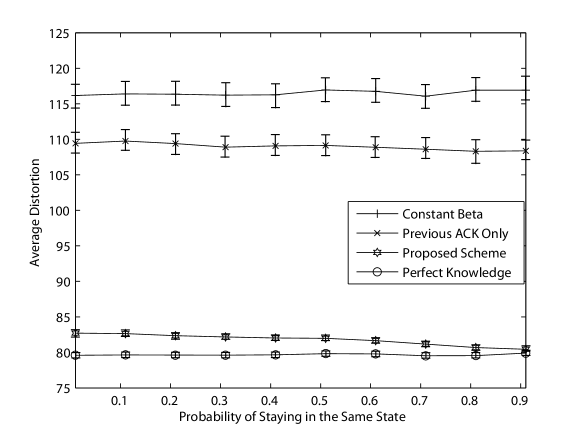
Figure 4: Average distortion vs. the probability of staying in the same state.

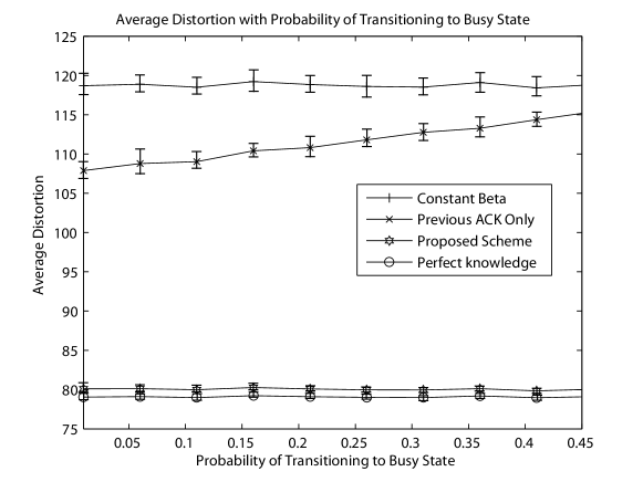
Figure 5: Average distortion vs. the probability of transitioning to the busy state.

We evaluate how the parameters in the transition matrix affect the average distortion. The transition matrix can be selected based on channel fading and primary usage. We ignore quantization errors caused by the limited number of states and assume the actual channel gain matches the state channel gain. Fig. 4 and Fig. 5 show the simulation results across $\mbox{Pr}\{X_{k+1}=v|X_{k}=v\}$ and $\mbox{Pr}\{X_{k+1}=z|X_{k}=v\}$, respectively. In Fig. 4, there are 5 states. $\epsilon=0.6$. $\mbox{Pr}\{X_{k+1}=z|X_{k}=v\}=0.05$. This example demonstrates the cognitive nature of the system. Our proposed method (i.e., method 2) approaches the method of using perfect knowledge of the channel state as $\mbox{Pr}\{X_{k+1}=v|X_{k}=v\}$ approaches 1. That is, the performance improves as the system dynamics slows down since it is easier to predict the actual system state. 5 states are used in Fig. 5. $\epsilon=0.6$. $\mbox{Pr}\{X_{k+1}=v|X_{k}=v\}=0.50$. From this figure, we can see that $\mbox{Pr}\{X_{k+1}=z|X_{k}=v\}$ has little impact to the performance of the proposed method. The reason for this observation is that increasing $\mbox{Pr}\{X_{k+1}=z|X_{k}=v\}$ will increase the likelihood the system transitions to the busy state, which has little affect on the average distortion when the channel is available and accessed.

4.3 Effects of the Parameters in the Observation Matrix

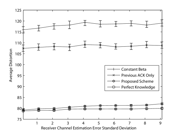
Figure 6: Average distortion vs. the receiver channel estimation standard deviation, $\sigma$.

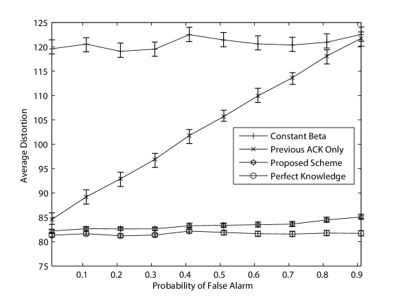
Figure 7: Average distortion vs. the sensor operating point, $\epsilon$.

The observation matrix is derived from the sensor operating point, $\epsilon$, and the standard deviation of the receiver channel estimation error, $\sigma$. Fig. 6 and Fig. 7 show how $\sigma$ and $\epsilon$ affect the average distortion. The following parameters are used in Fig. 6. There are 5 states, $\epsilon=0.6$, $\mbox{Pr}\{X_{k+1}=v|X_{k}=v\}=0.85$, and $\mbox{Pr}\{X_{k+1}=z|X_{k}=v\}=0.05$. We can see from Fig. 6, as the receiver estimation degrades, the acknowledgment provides less information on the actual channel gain and the average distortion of our method increases. $\epsilon$ and $\delta$ are related based on the sensor ROC, and adjusting $\epsilon$ implies a change to the system probability of collision requirement. In Fig. 7, $\mbox{Pr}\{X_{k+1}=v|X_{k}=v\}=0.85$, $\mbox{Pr}\{X_{k+1}=z|X_{k}=v\}=0.05$, and $\sigma=0.1$. This figure shows that the average distortion increases as the probability of false alarm increases.

4.4 Effects of the Transition Matrix on Channel Selection Policy

We consider a system with $N=2$ channels and $S=3$ states to evaluate the performance of the channel selection policy. We will use a spectrum utilization (SU) metric to evaluate the sensor policy performance. SU represents the percentage of time slots where an available channel was selected for sensing. SU is an important parameter when evaluating video QoS. The channel distortion is infinite when a channel is busy or not accessed. Improving the SU will reduce the percentage of time slots where a busy channel was selected for sensing thus improving the application layer QoS. The application layer QoS is improved using a two step process. First we select a channel to maximize SU thus reducing the large distortion introduced when the channel is unavailable. Second for an available and accessed channel, we select the intra refreshing rate to minimize distortion for a particular channel gain.

The two channels, channel $1$ and channel $2$, are simulated having the same number of states (i.e. quantized channel gains) and observation probabilities but asymmetric transition probabilities. Channel $2$ will have a higher primary usage than channel $1$. Based on previous observations, actions, and the POMDP derived policy the secondary transmitter/receiver pair dynamically selects the channel that will most likely maximize application layer QoS.

We evaluate SU and average distortion performance for three cases (1) POMDP channel selection, which is our proposed scheme, (2) randomly selecting channel $1$ or $2$ and using a constant $\beta=0.1$, which represents a non-adaptive scheme, and (3) using perfect knowledge of the system state, which represents the ideal case.

SU performance with varying transition matrix parameters is shown in Fig. 8 and Fig. 9. In both plots we only vary the transition matrix parameters of channel $1$. Both channels have equal observation matrix parameters $\epsilon^{1}=\epsilon^{2}=0.62$ and $\sigma^{1}=\sigma^{2}=0.1$.

In Fig. 8 we vary the probability channel $1$ stays busy, $\mbox{Pr}\{X_{k+1}^{1}=z|X_{k}^{1}=z\}$. $\mbox{Pr}\{X_{k+1}^{1}=z|X_{k}^{1}=v\}=0.2$. $\mbox{Pr}\{X_{k+1}^{2}=z|X_{k}^{2}=z\}=0.8$. $\mbox{Pr}\{X_{k+1}^{2}=z|X_{k}^{2}=v\}=0.6$. In Fig. 9 we vary the probability channel $1$ transitions to the busy state, $\mbox{Pr}\{X_{k+1}^{1}=z|X_{k}^{1}=v\}$. $\mbox{Pr}\{X_{k+1}^{1}=z|X_{k}^{1}=z\}=0.4$. $\mbox{Pr}\{X_{k+1}^{2}=z|X_{k}^{2}=z\}=0.8$. $\mbox{Pr}\{X_{k+1}^{2}=z|X_{k}^{2}=v\}=0.6$.

In both cases, the SU utilization of our scheme is greater than the non-adaptive scheme. Our proposed scheme senses the surrounding environment to learn and adapt channel selection. However it takes several time slots for the policy to learn the system state thus the performance of our scheme improves with slower transition dynamics. That is, our scheme approaches the perfect case as $\mbox{Pr}\{X_{k+1}^{1}=z|X_{k}^{1}=v\}$ approaches $0$ as is shown in Fig. 9. Our scheme provides closer to optimal performance when there is a large difference in channel availability between the two channels as it becomes easier to distinguish the better channel. This is demonstrated in Fig. 8 where the performance of our scheme is more optimal at low $\mbox{Pr}\{X_{k+1}^{1}=z|X_{k}^{1}=z\}$ relative to $\mbox{Pr}\{X_{k+1}^{2}=z|X_{k}^{2}=z\}$. In Fig. 10, we show the average distortion for the probability channel $1$ stays busy. The average distortion of our scheme is better than the non-adaptive scheme. Transition matrix parameters have little affect to the average distortion. Our scheme outperforms the non-adaptive scheme because our scheme will select the channel with the better channel gain and adapt the intra refreshing rate for the selected channel.

4.5 Effects of the Observation Matrix on Channel Selection Policy

SU with varying sensor operating point is shown in Fig. 11. $\mbox{Pr}\{X_{k+1}^{1}=z|X_{k}^{1}=z\}=0.4$. $\mbox{Pr}\{X_{k+1}^{1}=z|X_{k}^{1}=v\}=0.15$. $\mbox{Pr}\{X_{k+1}^{2}=z|X_{k}^{2}=z\}=0.6$. $\mbox{Pr}\{X_{k+1}^{2}=z|X_{k}^{2}=v\}=0.2$. Observation parameters are derived by operating characteristics of the secondary users and are not likely to be different for each channel. Thus both channels are simulated with symmetrical observation parameters, $\epsilon^{1}=\epsilon^{2}=\epsilon$ and $\sigma^{1}=\sigma^{2}=\sigma$. In Fig. 11 we vary the spectrum operating point $\epsilon$. In Fig. 12 we show the average distortion with varying $\epsilon$. The observation parameters are shown to have little affect on the SU and average distortion performance of our proposed scheme.

These simulation results demonstrate some interesting trends in the design and optimization of CR networks from a cross-layer design perspective. Adaptively adjusting the intra refreshing rate to accommodate time varying wireless channels is an effective way to reduce distortion. By using all previous actions and observations we can build an information state that becomes more accurate over time. Performance of using the information state to select the intra refreshing rate improves as the system dynamics slows down. In a CR environment the MAC access strategy is derived from the accuracy of the spectrum sensor. The total distortion is limited to the availability of the channel. Distortion performance will degrade if primary usage increases or a very low system tolerable probability of collision is required.

5 Conclusions and Future Work

In this paper, we have presented an integrated approach for multimedia transmission over cognitive radio networks. An important application layer parameter, intra refreshing rate, can be adjusted together with other parameters at other layers based on the sensed channel condition by the secondary users. A low complexity dynamic programming framework was presented to obtain the optimal intra refreshing policy. By modeling the system as a Markov process, we have derived a POMDP for optimal channel selection to minimize distortion while improving spectrum efficiency. Simulation results demonstrated the performance gain by using the adaptive transmission scheme. Future work is in progress to consider other QoS at the application layer.

Acknowledgment

We thank the reviewers for their detailed reviews and constructive comments, which have helped to improve the quality of this paper.

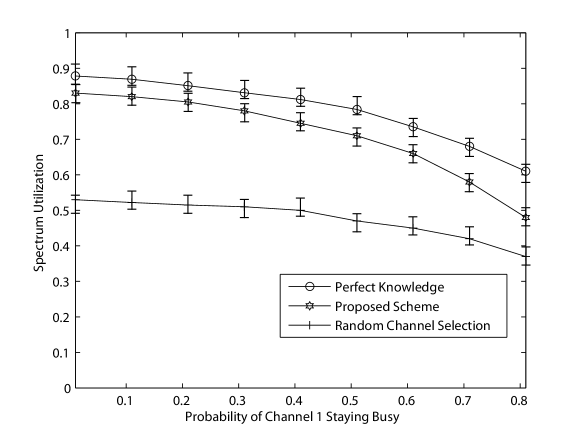
Figure 8: Two Channel Scenario: Spectrum utilization vs. the probability of staying in the busy state of channel 1.

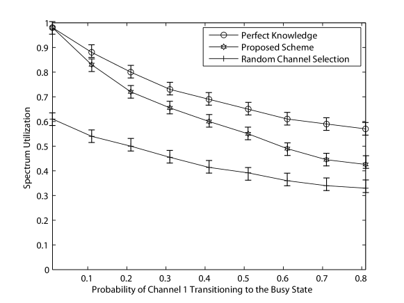
Figure 9: Two Channel Scenario: Spectrum utilization vs. the probability of transitioning to the busy state of channel 1.

Figure 10: Two Channel Scenario: Average distortion vs. the probability of staying in the busy state of channel 1.

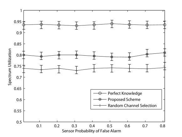
Figure 11: Two Channel Scenario: Spectrum utilization vs. the receiver channel estimation standard deviation, $\sigma$.

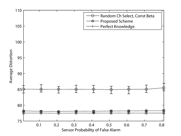
Figure 12: Two Channel Scenario: Average distortion vs. the receiver channel estimation standard deviation, $\sigma$.

References

- [1] J. Mitola, An Integrated Agent Architecture for Software Defined Radio. PhD thesis, 2000.
- [2] S. Haykin, “Cognitive radio: Brain-empowered wireless communications,” IEEE J. Sel. Areas Commun., vol. 23, pp. 201–220, Feb. 2005.
- [3] H. Su and X. Zhang, “Cross-layer based opportunistic mac protocols for qos provisionings over cognitive radio wireless networks,” IEEE J. Sel. Areas Commun., vol. 26, pp. 118–129, Jan. 2008.
- [4] H. Su and X. Zhang, “Opportunistic mac protocols for cognitive radio based wireless networks,” in Proc. IEEE the 41st Conference on Information Sciences and Systems (CISS 2007), (John Hopkings University, Baltimore, MD, USA), Mar. 2007.
- [5] H. Su and X. Zhang, “Cream-mac: An efficient cognitive radio-enabled multi-channel mac protocol for wireless networks,” in Proc. IEEE International Symposium on a World of Wireless, Mobile, and Multimedia Networks (WoWMoM 2008), (Newport Beach, California, USA), June 2008.
- [6] Q. Zhao and B. M. Sadler, “A survey of dynamic spectrum access,” IEEE Signal Proc. Mag., vol. 24, pp. 79–89, May 2007.
- [7] Z. Li, F. R. Yu, and M. Huang, “A distributed consensus-based cooperative spectrum sensing in cognitive radios,” IEEE Trans. Veh. Tech., 2010.
- [8] F. R. Yu, M. Huang, and H. Tang, “Biologically inspired consensus-based spectrum sensing in mobile ad hoc networks with cognitive radios,” IEEE Networks, 2010.
- [9] Q. Zhao, L. Tong, A. Swami, and Y. Chen, “Decentralized cognitive MAC for opportunistic spectrum access in ad hoc networks: A POMDP framework,” IEEE J. Sel. Areas Commun., vol. 25, pp. 589–600, Apr. 2007.
- [10] Y. Chen, Q. Zhao, and A. Swami, “Joint design and separation principle for opportunistic spectrum access in the presence of sensing errors,” IEEE Trans. Inform. Theory, vol. 54, May 2008.
- [11] G. Ganesan and Y. Li, “Cooperative spectrum sensing in cognitive radio, part I: two user networks,” IEEE Trans. Wireless Commun., vol. 6, pp. 2204–2213, June 2007.
- [12] G. Ganesan and Y. Li, “Cooperative spectrum sensing in cognitive radio - part II: multiuser networks,” IEEE Trans. Wireless Commun., vol. 6, pp. 2214–2222, June 2007.
- [13] W. Hu, D. Willkomm, G. Vlantis, M. Gerla, and A. Wolisz, “Dynamic frequency hopping communities for efficient IEEE 802.22 operation,” IEEE Comm. Magazine, vol. 45, pp. 80–87, May 2007.
- [14] Z. Ji and K. J. R. Liu, “Dynamic spectrum sharing: a game theoretical overview,” IEEE Comm. Mag., vol. 45, pp. 88–94, May 2007.
- [15] D. Zhang and Z. Tian, “Adaptive games for agile spectrum access based on extended kalman filtering,” IEEE J. Sel. Topics Signal Proc., vol. 1, pp. 79–90, Jun. 2007.
- [16] R. Etkin, A. Parekh, and D. Tse, “Spectrum sharing for unlicensed bands,” IEEE J. Sel. Areas Commun., vol. 25, pp. 517–528, Apr. 2007.
- [17] S. Geirhofer, L. Tong, and B. M. Sadler, “Cognitive radios for dynamic spectrum access - dynamic spectrum access in the time domain: Modeling and exploiting white space,” in IEEE Comm. Mag., vol. 45, pp. 66–72, May 2007.
- [18] P. Papadimitratos, S. Sankaranarayanan, and A. Mishra, “A bandwidth sharing approach to improve licensed spectrum utilization,” IEEE Comm. Mag., vol. 43, Dec. 2005.
- [19] M. van Der Schaar and S. S. N, “Cross-layer wireless multimedia transmission: challenges, principles, and new paradigms,” IEEE Wireless Comm., vol. 12, pp. 50–58, Aug. 2005.
- [20] S. Khan, Y. Peng, E. Steinbach, M. Sgroi, and W. Kellerer, “Application-driven cross-layer optimization for video streaming over wireless networks,” IEEE Comm. Mag., vol. 44, pp. 122–130, Jan. 2006.
- [21] J. M. Chapin and W. H. Lehr, “The path to market success for dynamic spectrum access technology,” IEEE Comm. Magazine, vol. 45, pp. 96–103, May 2007.
- [22] J. Tang and X. Zhang, “Quality-of-service driven power and rate adaptation over wireless links,” IEEE Trans. Wireless Commun., vol. 6, pp. 3058–3068, Aug. 2007.
- [23] Z. He, J. Cai, and C. Chen, “Joint source channel rate-distortion analysis for adaptive mode selection and rate control in wireless video coding,” IEEE Trans. Circ. Sys. Video Tech., vol. 12, pp. 511–523, June 2002.
- [24] A. Boukerche, Handbook of Algorithms for Wireless Networking and Mobile Computing (Chapman & Hall/Crc Computer & Information Science). Chapman & Hall/CRC, 2005.
- [25] F. Yu and V. Krishnamurthy, “Optimal joint session admission control in integrated wlan and cdma cellular networks with vertical handoff,” IEEE Trans. Mobile Comput., vol. 6, pp. 126–139, Jan. 2007.
- [26] J. Tang and X. Zhang, “Transmit selection diversity with maximal-ratio combining for multicarrier ds-cdma wireless networks over nakagami-m fading channels,” IEEE J. Sel. Areas Commun., vol. 24, pp. 104–112, Jan. 2006.
- [27] J. Tang and X. Zhang, “Cross-layer design of dynamic resource allocation of diverse qos guarantees for mimo-ofdm wireless networks,” in Proc. IEEE International Symposium on a World of Wireless, Mobile, and Multimedia Networks (WoWMoM 2005), (Taormina, Italy), June 2005.
- [28] J. Tang and X. Zhang, “Cross-layer resource allocation over wireless relay networks for quality of service provisioning,” IEEE J. Sel. Areas Commun., vol. 25, pp. 645–657, May 2007.
- [29] A. Boukerche, S. Hong, and T. Jacob, “An efficient synchronization scheme of multimedia streams in wireless and mobile systems,” IEEE Trans. Parallel Distrib. Syst., vol. 13, no. 9, pp. 911–923, 2002.
- [30] J. Tang and X. Zhang, “Clustering-based multi-channel mac protocols for qos-provisionings over vehicular ad hoc networks,” IEEE Trans. Veh. Tech., vol. 56, pp. 3309–3323, Nov. 2007.
- [31] F. Yu and V. Leung, “Mobility-based predictive call admission control and bandwidth reservation in wireless cellular networks,” Computer Networks, vol. 38, pp. 577–589, April 2002.
- [32] J. Tang and X. Zhang, “Cross-layer modeling for quality of service guarantees over wireless links,” IEEE Trans. Wireless Commun., vol. 6, pp. 4504–4512, Dec. 2007.
- [33] L. Ma, F. Yu, V. C. M. Leung, and T. Randhawa, “A new method to support UMTS/WLAN vertical handover using SCTP,” IEEE Wireless Commun., vol. 11, pp. 44–51, Aug. 2004.
- [34] X. Zhang and K. G. Shin, “Statistical analysis of feedback-synchronization signaling delay for multicast flow control,” in Proc. IEEE INFOCOM’2001, (Anchorage, Alaska, USA), Apr. 2001.
- [35] X. Zhang and K. G. Shin, “Markov-chain modeling for multicast signaling delay analysis,” IEEE/ACM Trans. Netw., vol. 12, pp. 667–680, Aug. 2004.
- [36] M. Van Der Schaar, D. S. Turaga, and R. Wong, “Classification-based system for cross-layer optimized wireless video transmission,” IEEE Trans. Multimedia, vol. 8, pp. 1082–1095, Oct. 2006.
- [37] D. Wu, S. Ci, and H. Wang, “Cross-layer optimization for video summary transmission over wireless networks,” IEEE J. Sel. Areas Commun., vol. 25, pp. 841–850, May 2007.
- [38] Y. S. Chan, J. W. Modestino, Q. Qu, and X. Fan, “An end-to-end embedded approach for multicast/broadcast of scalable video over multiuser CDMA wireless networks,” IEEE Trans. Multimedia, vol. 9, pp. 655–667, Apr. 2007.
- [39] A. R. Cassandra, Exact and Approximate Algorithms for Partially Observed Markov Decision Process. PhD thesis, Brown University, 1998.
- [40] H.-J. Lee, T. Chiang, and Y.-Q. Zhang, “Scalable rate control for MPEG-4 video,” IEEE Trans. Circ. Sys. Video Tech., vol. 10, pp. 878–894, Sep. 2000.
- [41] Z. He, Y. K. Kim, and S. K. Mitra, “Object-level bit allocation and scalable rate control for MPEG-4 video coding,” in Proc. of Workshop and Exhibition on MPEG-4, pp. 63–66, Jun. 2001.
- [42] K. Stuhlmuller, N. Farber, M. Link, and B. Girod, “Analysis of video transmission over lossy channels,” IEEE J. Sel. Areas Commun., vol. 18, pp. 1012–1032, Jun. 2000.
- [43] D. S. X. Zhang, K. G. Shin and D. Kandlur, “Scalable flow control for multicast abr services in atm networks,” IEEE/ACM Trans. Netw., vol. 10, pp. 67–85, Feb. 2002.
- [44] J. Y. Liao and J. Villasenor, “Adaptive intra block update for robust transmission of H.263,” IEEE Trans. Circ. Sys. Video Tech., vol. 10, pp. 30–35, Feb. 2000.
- [45] G. Cote, S. Shirani, and F. Kossentini, “Optimal mode selection and synchronization for robust video communications over error-prone networks,” IEEE J. Sel. Areas Commun., vol. 18, pp. 952–965, June 2000.
- [46] H. Tong and T. Brown, “Adaptive call admission control under quality of service constraints: a reinforcement learning solution,” IEEE J. Sel. Areas Commun., vol. 18, no. 2, pp. 209–221, 2000.
- [47] P. Bergamo, D. Maniezzo, A. Giovanardi, G. Mazini, and M. Zorzi, “Improved markov model for rayleigh fading envelope,” Electronics Letters, vol. 38, pp. 477–478, May 2002.
- [48] A. T. Hoang and M. Motani, “Buffer and channel adaptive transmission over fading channels with imperfect channel state information,” in Proc. IEEE WCNC’04, vol. 3, Mar. 2004.
- [49] W. Lovejoy, “A survey of algorithmic methods for partially observed Markov decision processes,” Ann. of Oper. Res., vol. 28, pp. 47–66, 1991.
- [50] W. Lovejoy, “Computationally feasible bounds for partially observed Markov decision processes,” Operations Research, vol. 39, pp. 162–175, Jan.–Feb. 1991.
- [51] V. Krishnamurthy, “Emission management for low probability intercept sensors in network centric warfare,” IEEE Trans. Aeros. Eelect. Systems, vol. 41, no. 1, pp. 133–152, 2005.
- [52] V. Krishnamurthy and D. Djonin, “Structured threshold policies for dynamic sensor scheduling - a partially observed Markov decision process approach,” IEEE Trans. Signal Proc., vol. 55, pp. 5069–5083, Oct. 2007.