Abstract

In our work on the development of model–independent data analysis methods for determining ratios between different couplings/cross sections of Weakly Interacting Massive Particles (WIMPs) by using measured recoil energies from direct Dark Matter detection experiments directly, it was assumed that the analyzed data sets are background–free, i.e., all events are WIMP signals. In this article, as a more realistic study, we take into account a fraction of possible residue background events, which pass all discrimination criteria and then mix with other real WIMP–induced events in our data sets.

Our simulations show that, assuming that the spin–dependent (SD) WIMP–nucleus interaction dominates over the spin–independent (SI) one, the maximal acceptable fraction of residue background events in the analyzed data sets for determining the ratio of the SD WIMP coupling on neutrons to that on protons is $\sim$ 20% – 40%; whereas considering a general combination of the SI and SD WIMP interactions, the maximal acceptable background ratio for determining the ratio between two SD WIMP couplings as well as the ratios of the SD cross section on protons (neutrons) to the SI one is $\sim$ 10% – 20%. Moreover, by considering different forms of background spectrum, we find that only background events in the lowest energy ranges could affect the reconstructions (significantly); those in high energy ranges would almost not change the reconstructed ratios or only very slightly.

1 Introduction

Currently, direct Dark Matter detection experiments searching for Weakly Interacting Massive Particles (WIMPs) are one of the promising methods for understanding the nature of Dark Matter (DM) and identifying them among new particles produced at colliders as well as reconstructing the (sub)structure of our Galactic halo [1, 2, 3, 4]. To this aim, model–independent methods for determining the WIMP mass [5, 6], the spin–independent (SI) WIMP coupling on nucleons [7, 8] as well as ratios between different WIMP couplings/cross sections [9, 10] from direct detection experiments have been developed.

These methods built basically on the work on the reconstruction of the (moments of the) one–dimensional velocity distribution function of halo WIMPs by using experimental data (measured recoil energies) directly [11]. The spectrum of recoil energy is proportional to an integral over the one–dimensional WIMP velocity distribution, $f_{1}(v)$, where $v$ is the absolute value of the WIMP velocity in the laboratory frame. Since this integral is in fact just the minus–first moment of the velocity distribution function, which can be estimated from experimental data directly [11, 6], by assuming that the spin–dependent (SD) WIMP–nucleus interaction dominates over the spin–independent one, an expression for determining the ratio between the SD WIMP coupling on neutrons and that on protons has been derived [9, 10]. Meanwhile, for a general combination of the SI and SD WIMP–nucleus interactions, by using detector materials with and without spin sensitivities on protons and/or on neutrons, a second expression for determining the ratio between two SD WIMP–nucleon couplings as well as two expressions for determining ratios of the SD WIMP–proton(neutron) cross section to the SI one have also been derived [9, 10]. It was found that, by combining experimental data sets with different target nuclei, the ratios between different WIMP couplings/cross sections can be determined without making any assumption about the velocity distribution of halo WIMPs nor prior knowledge about their mass [9, 10].

In the work on the development of these model–independent data analysis procedures for extracting information on WIMP couplings/cross sections from direct detection experiments, it was assumed that the analyzed data sets are background–free, i.e., all events are WIMP signals. Active background discrimination techniques should make this condition possible. For example, the ratio of the ionization to recoil energy, the so–called “ionization yield”, used in the CDMS-II experiment provides an event–by–event rejection of electron recoil events to be better than $10^{-4}$ misidentification [12]. By combining the “phonon pulse timing parameter”, the rejection ability of the misidentified electron recoils (most of them are “surface events” with sufficiently reduced ionization energies) can be improved to be $<10^{-6}$ [12]. Moreover, as demonstrated by the CRESST collaboration [13], by means of inserting a scintillating foil, which causes some additional scintillation light for events induced by $\alpha$-decay of ${}^{210}{\rm Po}$ and thus shifts the pulse shapes of these events faster than pulses induced by WIMP interactions in the crystal, the pulse shape discrimination (PSD) technique can then easily distinguish WIMP–induced nuclear recoils from those induced by backgrounds.

However, as the most important issue in all underground experiments, the signal identification ability and possible residue background events which pass all discrimination criteria and then mix with other real WIMP–induced events in analyzed data sets should also be considered. Therefore, in this article, as a more realistic study, we follow our works on the effects of residue background events in direct Dark Matter detection experiments [17, 18, 19] and want to study how well we could determine the ratios of WIMP–nucleon couplings/cross sections model–independently by using “impure” data sets and how “dirty” these data sets could be to be still useful.

The remainder of this article is organized as follows. In Sec. 2 I review briefly the model–independent methods for determining ratios between different WIMP–nucleon couplings/cross sections by using experimental data sets directly. In Sec. 3 the effects of residue background events in the analyzed data sets on the measured energy spectrum will be discussed. In Secs. 4 and 5 I show numerical results of the reconstruction of ratios of WIMP–nucleon couplings/cross sections by using mixed data sets with different fractions of residue background events based on Monte Carlo simulations. I conclude in Sec. 6. Some technical details will be given in an appendix.

2 Methods for determining ratios of WIMP–nucleon couplings/cross sections

In this section I review briefly the model–independent methods for determining the ratio of the SD WIMP coupling on neutrons to that on protons as well as the ratio between the SD and SI WIMP–proton cross sections. For more detailed illustrations and discussions about these precedures see [10].

2.1 Event rate for elastic WIMP–nucleus scattering

Considering the SI and SD WIMP–nucleus interactions together, the basic expression for the differential event rate for elastic WIMP–nucleus scattering can be given as [3, 10]:

$$\frac{dR}{dQ}=\frac{\rho_{0}}{2m_{\chi}m_{\rm r,N}^{2}}\bigg{[}\sigma_{0}^{\rm SI}F_{\rm SI}^{2}(Q)+\sigma_{0}^{\rm SD}F_{\rm SD}^{2}(Q)\bigg{]}\int_{v_{\rm min}}^{v_{\rm max}}\left[\frac{f_{1}(v)}{v}\right]dv~{}\!.$$ (1)

Here $R$ is the direct detection event rate, i.e., the number of events per unit time and unit mass of detector material, $Q$ is the energy deposited in the detector, $\rho_{0}$ is the WIMP density near the Earth, $\sigma_{0}^{\rm(SI,SD)}$ are the SI/SD total cross sections ignoring the form factor suppression and $F_{\rm(SI,SD)}(Q)$ are the elastic nuclear form factors for the SI/SD WIMP interactions, respectively, $f_{1}(v)$ is the one–dimensional velocity distribution function of the WIMPs impinging on the detector, $v$ is the absolute value of the WIMP velocity in the laboratory frame. The reduced mass $m_{\rm r,N}$ is defined by

$$m_{\rm r,N}\equiv\frac{m_{\chi}m_{\rm N}}{m_{\chi}+m_{\rm N}}~{}\!,$$ (2)

where $m_{\chi}$ is the WIMP mass and $m_{\rm N}$ that of the target nucleus. Finally, $v_{\rm min}$ is the minimal incoming velocity of incident WIMPs that can deposit the energy $Q$ in the detector:

$$v_{\rm min}=\alpha\sqrt{Q}~{}\!,$$ (3)

with the transformation constant

$$\alpha\equiv\sqrt{\frac{m_{\rm N}}{2m_{\rm r,N}^{2}}}~{}\!,$$ (4)

and $v_{\rm max}$ is the maximal WIMP velocity in the Earth’s reference frame, which is related to the escape velocity from our Galaxy at the position of the Solar system, $v_{\rm esc}~{}\>\raisebox{-3.01385pt}{$\stackrel{{\scriptstyle\textstyle>}}{{\sim}}$}\>~{}600$ km/s.

Through e.g., squark and Higgs exchanges with quarks, WIMPs could have a “scalar” interaction with nuclei. The SI scalar WIMP–nucleus cross section can be expressed as [3, 4]

$$\sigma_{0}^{\rm SI} = \left(\frac{4}{\pi}\right)m_{\rm r,N}^{2}\Big{[}Zf_{\rm p}+(A-Z)f_{\rm n}\Big{]}^{2}$$ (5)

$$\simeq \left(\frac{4}{\pi}\right)m_{\rm r,N}^{2}A^{2}|f_{\rm p}|^{2}$$

$$= A^{2}\left(\frac{m_{\rm r,N}}{m_{\rm r,p}}\right)^{2}\sigma_{\chi{\rm p}}^{\rm SI}~{}\!.$$

Here

$$\sigma_{\chi{\rm p}}^{\rm SI}=\left(\frac{4}{\pi}\right)m_{\rm r,p}^{2}|f_{\rm p}|^{2}$$ (6)

is the SI WIMP cross section on protons, $f_{\rm p(n)}$ are the effective $\chi\chi{\rm pp(nn)}$ four–point couplings, $A$ is the atomic mass number of the target nucleus, and $m_{\rm r,p}$ is the reduced mass of the WIMP mass $m_{\chi}$ and the proton mass $m_{\rm p}$. Note that I have used here the theoretical prediction for the lightest supersymmetric neutralino (and for all WIMPs which interact primarily through Higgs exchange) that the scalar couplings are approximately the same on protons and on neutrons: $f_{\rm n}\simeq f_{\rm p}$; the tiny mass difference between a proton and a neutron has also been neglected.

Isotope	$Z$	$J$	$\langle{\textstyle{S_{\rm p}}}\rangle$	$\langle{\textstyle{S_{\rm n}}}\rangle$	$-\langle{\textstyle{S_{\rm p}}}\rangle/\langle{\textstyle{S_{\rm n}}}\rangle$	$\langle{\textstyle{S_{\rm n}}}\rangle/\langle{\textstyle{S_{\rm p}}}\rangle$	Natural abundance (%)
${}^{19}{\rm F}$	9	1/2	0.441	$-$0.109	4.05	$-$0.25	100
${}^{23}{\rm Na}$	11	3/2	0.248	0.020	$-$12.40	0.08	100
${}^{35}{\rm Cl}$	17	3/2	$-$0.059	$-$0.011	$-$5.36	0.19	76
${}^{37}{\rm Cl}$	17	3/2	$-$0.058	0.050	1.16	$-$0.86	24
${}^{73}{\rm Ge}$	32	9/2	0.030	0.378	$-$0.08	12.6	7.8 / 86 (HDMS) [23]
${}^{127}{\rm I}$	53	5/2	0.309	0.075	$-$4.12	0.24	100
${}^{129}{\rm Xe}$	54	1/2	0.028	0.359	$-$0.08	12.8	26
${}^{131}{\rm Xe}$	54	3/2	$-$0.009	$-$0.227	$-$0.04	25.2	21

Table 1: List of the relevant spin values of the nuclei used for simulations presented in this paper. More details can be found in e.g., Refs. [3, 20, 21, 22].

On the other hand, through e.g., squark and Z boson exchanges with quarks, WIMPs could also couple to the spin of target nuclei, an “axial–vector” (spin–spin) interaction. The SD WIMP–nucleus cross section can be expressed as [3, 4]:

$$\sigma_{0}^{\rm SD}=\left(\frac{32}{\pi}\right)G_{F}^{2}~{}\!m_{\rm r,N}^{2}\left(\frac{J+1}{J}\right)\Big{[}\langle{\textstyle{S_{\rm p}}}\rangle a_{\rm p}+\langle{\textstyle{S_{\rm n}}}\rangle a_{\rm n}\Big{]}^{2}~{}\!.$$ (7)

Here $G_{F}$ is the Fermi constant, $J$ is the total spin of the target nucleus, $\langle{\textstyle{S_{\rm(p,n)}}}\rangle$ are the expectation values of the proton and neutron group spins, and $a_{\rm(p,n)}$ are the effective SD WIMP couplings on protons and on neutrons. Since for a proton or a neutron $J=\frac{1}{2}$ and $\langle{\textstyle{S_{\rm p}}}\rangle$ or $\langle{\textstyle{S_{\rm n}}}\rangle=\frac{1}{2}$, the SD WIMP cross section on protons or on neutrons can be given as

$$\sigma_{\chi{\rm(p,n)}}^{\rm SD}=\left(\frac{24}{\pi}\right)G_{F}^{2}~{}\!m_{\rm r,(p,n)}^{2}|a_{\rm(p,n)}|^{2}~{}\!.$$ (8)

As shown in Eq. (5), due to the coherence effect with the entire nucleus, the cross section for SI scalar WIMP–nucleus interaction scales approximately as the square of the atomic mass of the target nucleus. Hence, in most supersymmetric models, the SI cross section for nuclei with $A~{}\>\raisebox{-3.01385pt}{$\stackrel{{\scriptstyle\textstyle>}}{{\sim}}$}\>~{}30$ dominates over the SD one [3, 4]. However, as discussed in Refs. [24, 25, 26], in Universal Extra Dimension (UED) models, the SD WIMP interaction with nucleus is less suppressed and could be compatible or even larger than the SI one.

2.2 Only a dominant SD WIMP–nucleus cross section

Consider at first the case that the SD WIMP–nucleus interaction strongly dominates over the SI one and thus neglect the first SI term, $\sigma_{0}^{\rm SI}F_{\rm SI}^{2}(Q)$, in the bracket on the right–hand side of Eq. (1). By using a time–averaged recoil spectrum, and assuming that no directional information exists, the normalized one–dimensional velocity distribution function of halo WIMPs, $f_{1}(v)$, has been solved analytically [11] and, consequently, its generalized moments can be estimated by [11, 6]

$$\langle{\textstyle{v^{n}}}\rangle(v(Q_{\rm min}),v(Q_{\rm max})) = \int_{v(Q_{\rm min})}^{v(Q_{\rm max})}v^{n}f_{1}(v)~{}\!dv$$ (9)

$$= \alpha^{n}\left[\frac{2Q_{\rm min}^{(n+1)/2}r(Q_{\rm min})/F^{2}(Q_{\rm min})+(n+1)I_{n}(Q_{\rm min},Q_{\rm max})}{2Q_{\rm min}^{1/2}r(Q_{\rm min})/F^{2}(Q_{\rm min})+I_{0}(Q_{\rm min},Q_{\rm max})}\right]~{}\!.$$

Here $v(Q)=\alpha\sqrt{Q}$, $Q_{\rm(min,max)}$ are the experimental minimal and maximal cut–off energies of the data set, respectively,

$$r(Q_{\rm min})\equiv\left(\frac{dR}{dQ}\right)_{{\rm expt},~{}\!Q=Q_{\rm min}}$$ (10)

is an estimated value of the measured recoil spectrum $(dR/dQ)_{\rm expt}$ (before normalized by an experimental exposure, $\cal E$) at $Q=Q_{\rm min}$, and $I_{n}(Q_{\rm min},Q_{\rm max})$ can be estimated through the sum:

$$I_{n}(Q_{\rm min},Q_{\rm max})=\sum_{a=1}^{N_{\rm tot}}\frac{Q_{a}^{(n-1)/2}}{F^{2}(Q_{a})}~{}\!,$$ (11)

where the sum runs over all events in the data set that satisfy $Q_{a}\in[Q_{\rm min},Q_{\rm max}]$ and $N_{\rm tot}$ is the number of such events. Then, since the integral on the right–hand side of Eq. (1) is just the minus–first generalized moment of the velocity distribution function, $\langle{\textstyle{v^{-1}}}\rangle$, which can be estimated by Eq. (9), by setting $Q=Q_{\rm min}$ and using the definition (4) of $\alpha$, one can obtain straightforwardly that

$$\rho_{0}\sigma_{0}^{\rm SD}=\left(\frac{1}{{\cal E}}\right)m_{\chi}m_{\rm r,N}\sqrt{\frac{m_{\rm N}}{2}}\left[\frac{2Q_{\rm min}^{1/2}r(Q_{\rm min})}{F_{\rm SD}^{2}(Q_{\rm min})}+I_{0}\right]~{}\!.$$ (12)

Now, in order to eliminate $\rho_{0}$ here, we combine two experimental data sets with different target nuclei, $X$ and $Y$. By substituting the expression (7) for $\sigma_{0}^{\rm SD}$ into Eq. (12) and using again the definition (4) of $\alpha$ for both target nuclei, the ratio between two SD WIMP–nucleon couplings has been solved analytically as [9, 10]

$$\left(\frac{a_{\rm n}}{a_{\rm p}}\right)_{\pm,n}^{\rm SD}=-\frac{\langle{\textstyle{S_{\rm p}}}\rangle_{X}\pm\langle{\textstyle{S_{\rm p}}}\rangle_{Y}\left({\cal R}_{J,n,X}/{\cal R}_{J,n,Y}\right)}{\langle{\textstyle{S_{\rm n}}}\rangle_{X}\pm\langle{\textstyle{S_{\rm n}}}\rangle_{Y}\left({\cal R}_{J,n,X}/{\cal R}_{J,n,Y}\right)}~{}\!,~{}~{}~{}~{}~{}~{}~{}~{}~{}~{}~{}~{}~{}~{}~{}~{}n\neq 0.$$ (13)

Here I have used the following relation [6]:

$$\frac{\alpha_{X}}{\alpha_{Y}}=\frac{{\cal R}_{n,Y}}{{\cal R}_{n,X}}~{}\!,$$ (14)

and defined

$${\cal R}_{J,n,X}\equiv\left[\Bigg{(}\frac{J_{X}}{J_{X}+1}\Bigg{)}\frac{{\cal R}_{\sigma,X}}{{\cal R}_{n,X}}\right]^{1/2}~{}\!,$$ (15)

with

$${\cal R}_{\sigma,X}\equiv\frac{1}{{\cal E}_{X}}\left[\frac{2Q_{{\rm min},X}^{1/2}r_{X}(Q_{{\rm min},X})}{F_{X}^{2}(Q_{{\rm min},X})}+I_{0,X}\right]~{}\!,$$ (16)

and

$${\cal R}_{n,X}\equiv\left[\frac{2Q_{{\rm min},X}^{(n+1)/2}r_{X}(Q_{{\rm min},X})/F_{X}^{2}(Q_{{\rm min},X})+(n+1)I_{n,X}}{2Q_{{\rm min},X}^{1/2}r_{X}(Q_{{\rm min},X})/F_{X}^{2}(Q_{{\rm min},X})+I_{0,X}}\right]^{1/n}~{}\!;$$ (17)

${\cal R}_{J,n,Y}$, ${\cal R}_{\sigma,Y}$, and ${\cal R}_{n,Y}$ can be defined analogously; $F_{(X,Y)}(Q)$ are the form factors of the nucleus $X$ and $Y$, $r_{(X,Y)}(Q_{{\rm min},(X,Y)})$ refer to the counting rates for the target $X$ and $Y$ at the respective lowest recoil energies included in the analysis, and ${\cal E}_{(X,Y)}$ are the experimental exposures with the target $X$ and $Y$. Note that, firstly, Eq. (13) can be used once positive signals are observed in two (or more) experiments; information on the local WIMP density $\rho_{0}$, on the velocity distribution function of incident WIMPs, $f_{1}(v)$, as well as on the WIMP mass $m_{\chi}$ are not necessary. Secondly, because the couplings in Eq. (7) are squared, we have two solutions for $a_{\rm n}/a_{\rm p}$ here; if exact “theory” values for ${\cal R}_{J,n,(X,Y)}$ are taken, these solutions coincide for

$$\left(\frac{a_{\rm n}}{a_{\rm p}}\right)_{+,n}^{\rm SD}=\left(\frac{a_{\rm n}}{a_{\rm p}}\right)_{-,n}^{\rm SD}=\left\{\begin{array}[]{l l l}\displaystyle-\frac{\langle{\textstyle{S_{\rm p}}}\rangle_{X}}{\langle{\textstyle{S_{\rm n}}}\rangle_{X}}~{}\!,&{}{}{}{}{}{}{}{}&{\rm for}~{}{\cal R}_{J,n,X}=0~{}\!,\\ \\ \displaystyle-\frac{\langle{\textstyle{S_{\rm p}}}\rangle_{Y}}{\langle{\textstyle{S_{\rm n}}}\rangle_{Y}}~{}\!,&&{\rm for}~{}{\cal R}_{J,n,Y}=0~{}\!,\end{array}\right.$$ (18)

which depends only on properties of two used target nuclei (see Table 1). Moreover, it can be found from Eq. (13) that one of these two solutions has a pole at the middle of two intersections, which depends simply on the signs of $\langle{\textstyle{S_{\rm n}}}\rangle_{X}$ and $\langle{\textstyle{S_{\rm n}}}\rangle_{Y}$: since ${\cal R}_{J,n,X}$ and ${\cal R}_{J,n,Y}$ are always positive, if both $\langle{\textstyle{S_{\rm n}}}\rangle_{X}$ and $\langle{\textstyle{S_{\rm n}}}\rangle_{Y}$ are positive or negative, the “$-$ (minus)” solution $(a_{\rm n}/a_{\rm p})^{\rm SD}_{-,n}$ will diverge and the “$+$ (plus)” solution $(a_{\rm n}/a_{\rm p})^{\rm SD}_{+,n}$ will be the “inner” solution; in contrast, if the signs of $\langle{\textstyle{S_{\rm n}}}\rangle_{X}$ and $\langle{\textstyle{S_{\rm n}}}\rangle_{Y}$ are opposite, the “$-$ (minus)” solution will be the “inner” solution.

On the other hand, it has been found [10] that, in order to reduce the statistical uncertainty on $(a_{\rm n}/a_{\rm p})^{\rm SD}_{\pm,n}$ estimated by Eq. (13),. one can practically use the estimate of the counting rate, instead of at the experimental minimal cut–off energy, at the shifted point $Q_{s,1}$ (from the central point of the first bin, $Q_{1}$) defined by

$$Q_{s,1}=Q_{1}+\frac{1}{k_{1}}\ln\left[\frac{\sinh(k_{1}b_{1}/2)}{k_{1}b_{1}/2}\right]~{}\!,$$ (19)

where $k_{1}$ is the logarithmic slope of the reconstructed recoil spectrum in the first $Q-$bin and $b_{1}$ is the bin width. Then, according to Eq. (A9), the measured recoil spectrum at $Q=Q_{s,1}$ can be estimated by

$$r(Q_{s,1})=\left(\frac{dR}{dQ}\right)_{{\rm expt},~{}\!1,~{}\!Q=Q_{s,1}}=r_{1}=\frac{N_{1}}{b_{1}}~{}\!,$$ (20)

where $N_{1}$ is the event number in the first bin.

As shown in Ref. [10], the statistical uncertainties on $(a_{\rm n}/a_{\rm p})^{\rm SD}_{\pm,n}$ estimated with different $n$ (namely with different moments of the WIMP velocity distribution function) with $r_{(X,Y)}(Q_{s,1,(X,Y)})$ are clearly reduced and, interestingly, almost equal. Therefore, since

$${\cal R}_{J,-1,X}=\left[\left(\frac{J_{X}}{J_{X}+1}\right)\frac{2~{}\!r_{X}(Q_{s,1,X})}{{\cal E}_{X}F_{X}^{2}(Q_{s,1,X})}\right]^{1/2}~{}\!,$$ (21)

one would need practically only events in the lowest energy ranges for estimating $a_{\rm n}/a_{\rm p}$. And, consequently, one has to estimate the values of form factors only at $Q=Q_{s,1}$, and the zero momentum transfer approximation $F^{2}(Q\simeq 0))\simeq 1$ can then be used.

2.3 Combination of the SI and SD cross sections

Now I consider the case with a non–negligible SI WIMP–nucleus cross section. At first, by combining Eqs. (5), (7), and (8), we can find

$$\frac{\sigma_{0}^{\rm SD}}{\sigma_{0}^{\rm SI}}=\left(\frac{32}{\pi}\right)G_{F}^{2}~{}\!m_{\rm r,p}^{2}\Bigg{(}\frac{J+1}{J}\Bigg{)}\left[\frac{\langle{\textstyle{S_{\rm p}}}\rangle+\langle{\textstyle{S_{\rm n}}}\rangle(a_{\rm n}/a_{\rm p})}{A}\right]^{2}\frac{|a_{\rm p}|^{2}}{\sigma_{\chi{\rm p}}^{\rm SI}}={\cal C}_{\rm p}\left(\frac{\sigma_{\chi{\rm p}}^{\rm SD}}{\sigma_{\chi{\rm p}}^{\rm SI}}\right)~{}\!,$$ (22)

where I have defined

$${\cal C}_{\rm p}\equiv\frac{4}{3}\left(\frac{J+1}{J}\right)\left[\frac{\langle{\textstyle{S_{\rm p}}}\rangle+\langle{\textstyle{S_{\rm n}}}\rangle(a_{\rm n}/a_{\rm p})}{A}\right]^{2}~{}\!.$$ (23)

Then the expression (1) for the differential event rate can be rewritten as

$$\left(\frac{dR}{dQ}\right)_{\rm expt}={\cal E}A^{2}\!\left(\frac{\rho_{0}\sigma_{\chi{\rm p}}^{\rm SI}}{2m_{\chi}m_{\rm r,p}^{2}}\right)\!\!\left[F_{\rm SI}^{2}(Q)+\left(\frac{\sigma_{\chi{\rm p}}^{\rm SD}}{\sigma_{\chi{\rm p}}^{\rm SI}}\right){\cal C}_{\rm p}F_{\rm SD}^{2}(Q)\right]\int_{v_{\rm min}}^{v_{\rm max}}\left[\frac{f_{1}(v)}{v}\right]dv~{}\!.$$ (24)

Set $Q=Q_{\rm min}$. One can find straightforwardly that, for this general case, Eq. (12) becomes to

$$\rho_{0}\left[A^{2}\left(\frac{m_{\rm r,N}}{m_{\rm r,p}}\right)^{2}\sigma_{\chi{\rm p}}^{\rm SI}\right]=\left(\frac{1}{{\cal E}}\right)m_{\chi}m_{\rm r,N}\sqrt{\frac{m_{\rm N}}{2}}\left[\frac{2Q_{\rm min}^{1/2}r(Q_{\rm min})}{F^{\prime 2}(Q_{\rm min})}+I_{0}\right]~{}\!,$$ (25)

where $I_{n}$ should be estimated by Eq. (11) with the replacement of $F^{2}(Q)$ by $F^{\prime 2}(Q)\equiv F_{\rm SI}^{2}(Q)+\left(\sigma_{\chi{\rm p}}^{\rm SD}/\sigma_{\chi{\rm p}}^{\rm SI}\right){\cal C}_{\rm p}F_{\rm SD}^{2}(Q)$.

By combining two targets $X$ and $Y$ and using the relation (14) for $\alpha_{X}/\alpha_{Y}$ with $n=-1$, the ratio of the SD WIMP–proton cross section to the SI one has been solved analytically as [10]

$$\frac{\sigma_{\chi{\rm p}}^{\rm SD}}{\sigma_{\chi{\rm p}}^{\rm SI}}=\frac{F_{{\rm SI},Y}^{2}(Q_{{\rm min},Y})({\cal R}_{m,X}/{\cal R}_{m,Y})-F_{{\rm SI},X}^{2}(Q_{{\rm min},X})}{{\cal C}_{{\rm p},X}F_{{\rm SD},X}^{2}(Q_{{\rm min},X})-{\cal C}_{{\rm p},Y}F_{{\rm SD},Y}^{2}(Q_{{\rm min},Y})({\cal R}_{m,X}/{\cal R}_{m,Y})}~{}\!,$$ (26)

where $m_{(X,Y)}\propto A_{(X,Y)}$ has been assumed, ${\cal C}_{{\rm p},(X,Y)}$ have been defined in Eq. (23), and

$${\cal R}_{m,X}\equiv\frac{r_{X}(Q_{{\rm min},X})}{{\cal E}_{X}m_{X}^{2}}~{}\!.$$ (27)

As the estimator (13) for $a_{\rm n}/a_{\rm p}$, one can use Eq. (26) to estimate $\sigma_{\chi{\rm p}}^{\rm SD}/\sigma_{\chi{\rm p}}^{\rm SI}$ without a prior knowledge of the WIMP mass $m_{\chi}$. Moreover, since ${\cal C}_{{\rm p},(X,Y)}$ depend only on the nature of the detector materials, $\sigma_{\chi{\rm p}}^{\rm SD}/\sigma_{\chi{\rm p}}^{\rm SI}$ is practically only a function of ${\cal R}_{m,(X,Y)}$, i.e., the counting rate at the experimental minimal cut–off energies, which can be estimated by using events in the lowest available energy ranges.

Meanwhile, for the general combination of the SI and SD WIMP–nucleus cross sections, the $a_{\rm n}/a_{\rm p}$ ratio appearing in Eq. (23) has been solved analytically by introducing a third nucleus with only an SI sensitivity: $\langle{\textstyle{S_{\rm p}}}\rangle_{Z}=\langle{\textstyle{S_{\rm n}}}\rangle_{Z}=0$, i.e., ${\cal C}_{{\rm p},Z}=0$ as [10]

$$\left(\frac{a_{\rm n}}{a_{\rm p}}\right)_{\pm}^{\rm SI+SD} = \frac{-\left(c_{{\rm p},X}s_{{\rm n/p},X}-c_{{\rm p},Y}s_{{\rm n/p},Y}\right)\pm\sqrt{c_{{\rm p},X}c_{{\rm p},Y}}\left|s_{{\rm n/p},X}-s_{{\rm n/p},Y}\right|}{c_{{\rm p},X}s_{{\rm n/p},X}^{2}-c_{{\rm p},Y}s_{{\rm n/p},Y}^{2}}$$ (34)

$$= \left\{\begin{array}[]{l l l}\\ \displaystyle-\frac{\sqrt{c_{{\rm p},X}}\mp\sqrt{c_{{\rm p},Y}}}{\sqrt{c_{{\rm p},X}}s_{{\rm n/p},X}\mp\sqrt{c_{{\rm p},Y}}s_{{\rm n/p},Y}}~{}\!,&{}{}{}{}{}{}{}{}&({\rm for}~{}s_{{\rm n/p},X}>s_{{\rm n/p},Y}),\\ {}\\ {}\\ \displaystyle-\frac{\sqrt{c_{{\rm p},X}}\pm\sqrt{c_{{\rm p},Y}}}{\sqrt{c_{{\rm p},X}}s_{{\rm n/p},X}\pm\sqrt{c_{{\rm p},Y}}s_{{\rm n/p},Y}}~{}\!,&&({\rm for}~{}s_{{\rm n/p},X}<s_{{\rm n/p},Y}).\\ {}\\ \end{array}\right.$$

Here I have defined

$$c_{{\rm p},X}\equiv\frac{4}{3}\Bigg{(}\frac{J_{X}+1}{J_{X}}\Bigg{)}\left[\frac{\langle{\textstyle{S_{\rm p}}}\rangle_{X}}{A_{X}}\right]^{2}\left[F_{{\rm SI},Z}^{2}(Q_{{\rm min},Z})\left(\frac{{\cal R}_{m,Y}}{{\cal R}_{m,Z}}\right)\!-F_{{\rm SI},Y}^{2}(Q_{{\rm min},Y})\right]\!F_{{\rm SD},X}^{2}(Q_{{\rm min},X})~{}\!,$$ (35a)

$$c_{{\rm p},Y}\equiv\frac{4}{3}\Bigg{(}\frac{J_{Y}+1}{J_{Y}}\Bigg{)}\left[\frac{\langle{\textstyle{S_{\rm p}}}\rangle_{Y}}{A_{Y}}\right]^{2}\left[F_{{\rm SI},Z}^{2}(Q_{{\rm min},Z})\left(\frac{{\cal R}_{m,X}}{{\cal R}_{m,Z}}\right)\!-F_{{\rm SI},X}^{2}(Q_{{\rm min},X})\right]\!F_{{\rm SD},Y}^{2}(Q_{{\rm min},Y})~{}\!,$$ (35b)

and

$$s_{{\rm n/p},X}\equiv\frac{\langle{\textstyle{S_{\rm n}}}\rangle_{X}}{\langle{\textstyle{S_{\rm p}}}\rangle_{X}}~{}\!.$$ (36)

Note that, firstly, $(a_{\rm n}/a_{\rm p})_{\pm}^{\rm SI+SD}$ and $c_{{\rm p},(X,Y)}$ given in Eqs. (34), (35a), and (35b) are functions of only $r_{(X,Y,Z)}(Q_{{\rm min},(X,Y,Z)})$ (or $r_{(X,Y,Z)}(Q_{s,1,(X,Y,Z)})$), which can be estimated with events in the lowest energy ranges. Secondly, while the decision of the inner solution of $(a_{\rm n}/a_{\rm p})_{\pm,n}^{\rm SD}$ depends on the signs of $\langle{\textstyle{S_{\rm n}}}\rangle_{X}$ and $\langle{\textstyle{S_{\rm n}}}\rangle_{Y}$, the decision with $(a_{\rm n}/a_{\rm p})_{\pm}^{\rm SI+SD}$ depends not only on the signs of $s_{{\rm n/p},X}=\langle{\textstyle{S_{\rm n}}}\rangle_{X}/\langle{\textstyle{S_{\rm p}}}\rangle_{X}$ and $s_{{\rm n/p},Y}=\langle{\textstyle{S_{\rm n}}}\rangle_{Y}/\langle{\textstyle{S_{\rm p}}}\rangle_{Y}$, but also on the order of the two targets. For e.g., a Ge + Cl combination, since $s_{{\rm n/p},^{73}{\rm Ge}}=12.6>s_{{\rm n/p},^{37}{\rm Cl}}=-0.86$, one should use the upper expression in the second line of Eq. (34), and since $s_{{\rm n/p},^{73}{\rm Ge}}$ and $s_{{\rm n/p},^{37}{\rm Cl}}$ have the opposite signs, the “$-$ (minus)” solution of this expression (or the “$+$ (plus)” solution of the expression in the first line) is the inner solution. In contrast, for the F + I combination used in our simulations, since $s_{{\rm n/p},^{19}{\rm F}}=-0.247<s_{{\rm n/p},^{127}{\rm I}}=0.243$ and since $s_{{\rm n/p},^{19}{\rm F}}$ and $s_{{\rm n/p},^{127}{\rm I}}$ have the opposite signs, the “$-$ (minus)” solution of the lower expression in the second line of Eq. (34) (or the “$-$ (minus)” solution of the expression in the first line) is then the inner solution.

Furthermore, in order to reduce the statistical uncertainty, one can choose at first a nucleus with only an SI sensitivity as the second target: $\langle{\textstyle{S_{\rm p}}}\rangle_{Y}=\langle{\textstyle{S_{\rm n}}}\rangle_{Y}=0$, i.e., ${\cal C}_{{\rm p},Y}=0$. The expression in Eq. (26) can thus be reduced to

$$\frac{\sigma_{\chi{\rm p}}^{\rm SD}}{\sigma_{\chi{\rm p}}^{\rm SI}}=\frac{F_{{\rm SI},Y}^{2}(Q_{{\rm min},Y})({\cal R}_{m,X}/{\cal R}_{m,Y})-F_{{\rm SI},X}^{2}(Q_{{\rm min},X})}{{\cal C}_{{\rm p},X}F_{{\rm SD},X}^{2}(Q_{{\rm min},X})}~{}\!.$$ (37)

Then we choose a nucleus with (much) larger proton (or neutron) group spin as the first target: $\langle{\textstyle{S_{\rm p}}}\rangle_{X}\gg\langle{\textstyle{S_{\rm n}}}\rangle_{X}\simeq 0$, in order to eliminate the $a_{\rm n}/a_{\rm p}$ dependence of ${\cal C}_{{\rm p},X}$ given in Eq. (23):

$${\cal C}_{{\rm p},X}\simeq\frac{4}{3}\Bigg{(}\frac{J_{X}+1}{J_{X}}\Bigg{)}\left[\frac{\langle{\textstyle{S_{\rm p}}}\rangle_{X}}{A_{X}}\right]^{2}~{}\!.$$ (39)

3 Effects of residue background events

In this section I first show some numerical results of the energy spectrum of WIMP recoil signals mixed with a few background events. For generating WIMP–induced signals, we use the shifted Maxwellian velocity distribution [2, 3, 11]:

$$f_{1,{\rm sh}}(v)=\frac{1}{\sqrt{\pi}}\left(\frac{v}{v_{\rm e}v_{0}}\right)\bigg{[}e^{-(v-v_{\rm e})^{2}/v_{0}^{2}}-e^{-(v+v_{\rm e})^{2}/v_{0}^{2}}\bigg{]}~{}\!,$$ (40)

with $v_{0}\simeq 220~{}{\rm km/s}$ and $v_{\rm e}=1.05~{}\!v_{0}$, which are the Sun’s orbital velocity and the Earth’s velocity in the Galactic frame, respectively; the maximal cut–off of the velocity distribution function has been set as $v_{\rm max}=700$ km/s. The commonly used elastic nuclear form factor for the SI WIMP–nucleus cross section [27, 3, 4]:

$$F_{\rm SI}^{2}(Q)=\left[\frac{3j_{1}(qR_{1})}{qR_{1}}\right]^{2}e^{-(qs)^{2}}$$ (41)

as well as the thin–shell form factor for the SD WIMP cross section [2, 28, 10]:

$$F_{\rm SD}^{2}(Q) = \left\{\begin{array}[]{l l l}j_{0}^{2}(qR_{1})~{}\!,&{}{}{}{}{}{}{}{}&{\rm for}~{}qR_{1}\leq 2.55~{}{\rm or}~{}qR_{1}\geq 4.5~{}\!,\\ {\rm const.}\simeq 0.047~{}\!,&&{\rm for}~{}2.55\leq qR_{1}\leq 4.5\end{array}\right.$$ (44)

will also be used. Meanwhile, in order to check the need of a prior knowledge about an (exact) form of the residue background spectrum, two forms for the background spectrum have been considered. The simplest choice is a constant spectrum:

$$\left(\frac{dR}{dQ}\right)_{\rm bg,const}=1~{}\!.$$ (45)

More realistically, we use the target–dependent exponential form introduced in Ref. [17] for the residue background spectrum:

$$\left(\frac{dR}{dQ}\right)_{\rm bg,ex}=\exp\left(-\frac{Q/{\rm keV}}{A^{0.6}}\right)~{}\!.$$ (46)

Here $Q$ is the recoil energy, $A$ is the atomic mass number of the target nucleus. The power index of $A$, 0.6, is an empirical constant, which has been chosen so that the exponential background spectrum is somehow similar to, but still different from the expected recoil spectrum of the target nucleus; otherwise, there is in practice no difference between the WIMP scattering and background spectra. Note that, among different possible choices, we use in our simulations the atomic mass number $A$ as the simplest, unique characteristic parameter in the general analytic form (46) for defining the residue background spectrum for different target nuclei. However, it does not mean that the (superposition of the real) background spectra would depend simply/primarily on $A$ or on the mass of the target nucleus, $m_{\rm N}$. In other words, it is practically equivalent to use expression (46) or $(dR/dQ)_{\rm bg,ex}=e^{-Q/13.5~{}{\rm keV}}$ directly for a ${}^{76}{\rm Ge}$ target.

Note also that, firstly, as argued in Ref. [17], two forms of background spectrum given above are rather naive; however, since we consider here only a few residue background events induced by perhaps two or more different sources, which pass all discrimination criteria, and then mix with other WIMP–induced events in our data sets of ${\cal O}(50)$ total events, exact forms of different background spectra are actually not very important and these two spectra, in particular, the exponential one, should practically not be unrealistic. Secondly, as demonstrated in Ref. [10] and reviewed in the previous section, the model–independent data analysis procedures for determining ratios between different WIMP–nucleon couplings/cross sections require only measured recoil energies (induced mostly by WIMPs and occasionally by background sources) from direct detection experiments. Therefore, for applying these methods to future real data, a prior knowledge about (different) background source(s) is not required at all.

Moreover, for our numerical simulations presented here as well as in the next two sections, the actual numbers of signal and background events in each simulated experiment are Poisson–distributed around their expectation values independently; and the total event number recorded in one experiment is then the sum of these two numbers. Additionally, we assumed that all experimental systematic uncertainties as well as the uncertainty on the measurement of the recoil energy could be ignored. The energy resolution of most existing detectors is so good that its error can be neglected compared to the statistical uncertainty for the foreseeable future with pretty few events.

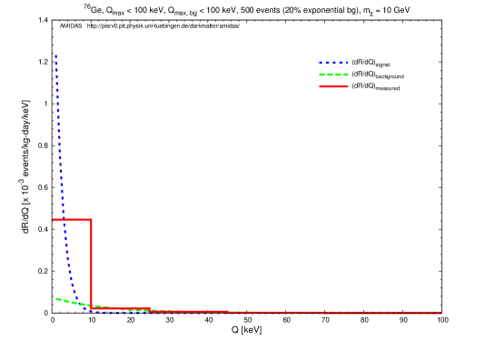
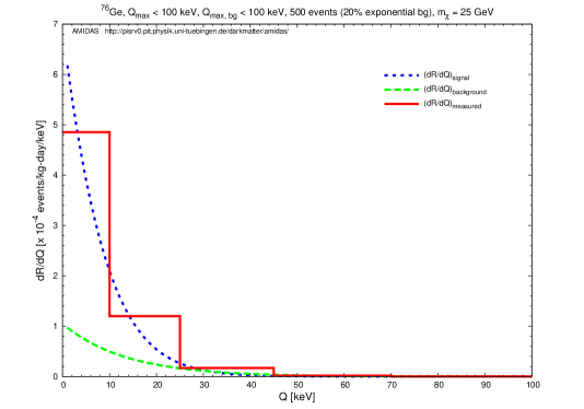
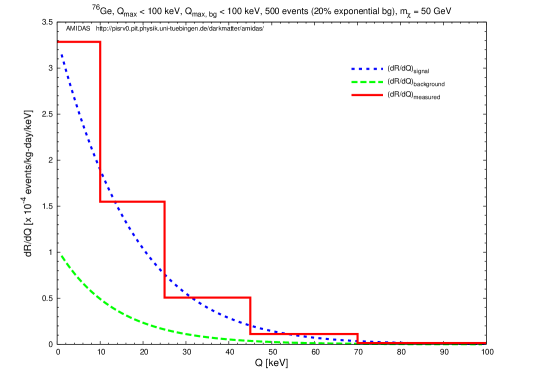
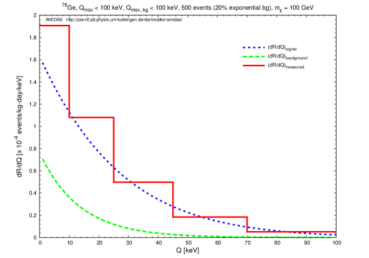
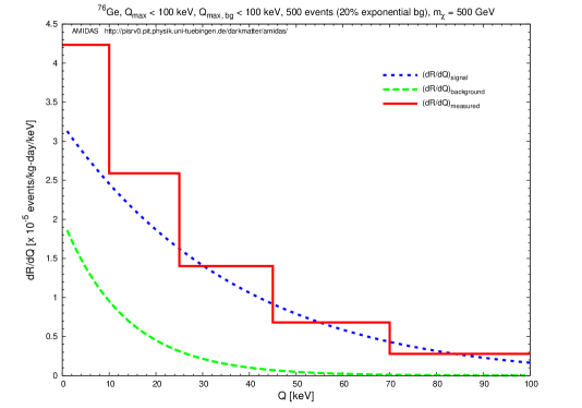
Figure 1: Measured energy spectra (solid red histograms) for a ${}^{76}{\rm Ge}$ target with six different WIMP masses: 10, 25, 50, 100, 250, and 500 GeV. The dotted blue curves are the elastic WIMP–nucleus scattering spectra, whereas the dashed green curves are the exponential background spectra normalized to fit to the chosen background ratio, which has been set as 20% here. The experimental threshold energies have been assumed to be negligible and the maximal cut–off energies are set as 100 keV. The background windows have been assumed to be the same as the experimental possible energy ranges. 5,000 experiments with 500 total events on average in each experiment have been simulated. See the text for further details (plots from Ref. [17]).

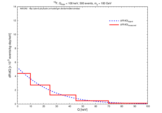
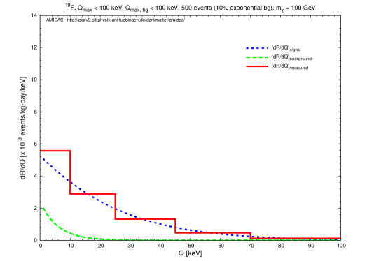
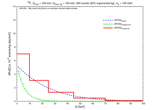
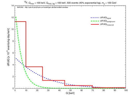
Figure 2: As in Figs. 1, except that a ${}^{19}{\rm F}$ target has been used, the input WIMP mass has been fixed as 100 GeV, and four different background ratios: no background (top left), 10% (top right), 20% (bottom left), and 40% (bottom right) are shown here.

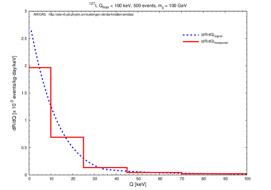
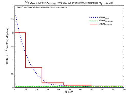
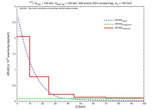
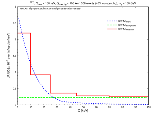
Figure 3: As in Figs. 2, except that an ${}^{127}{\rm I}$ target and the constant background spectrum have been used here.

In Figs. 1 I show measured energy spectra (solid red histograms) for a ${}^{76}{\rm Ge}$ target with six different WIMP masses: 10, 25, 50, 100, 250, and 500 GeV based on Monte Carlo simulations. The dotted blue curves are the elastic WIMP–nucleus scattering spectra, whereas the dashed green curves are the exponential background spectra given in Eq. (46), which have been normalized so that the ratios of the areas under these background spectra to those under the (dotted blue) WIMP scattering spectra are equal to the background–signal ratio in the whole data sets (e.g., 20% backgrounds to 80% signals shown in Figs. 1). The experimental threshold energies have been assumed to be negligible and the maximal cut–off energies are set as 100 keV. The background windows (the possible energy ranges in which residue background events exist) have been assumed to be the same as the experimental possible energy ranges. 5,000 experiments with 500 total events on average in each experiment have been simulated.

Remind that the measured energy spectra shown here are averaged over the simulated experiments. Five bins with linear increased bin widths have been used for binning generated signal and background events. As argued in Ref. [11], for reconstructing the one–dimensional WIMP velocity distribution function, this unusual, particular binning has been chosen in order to accumulate more events in high energy ranges and thus to reduce the statistical uncertainties in high velocity ranges. However, as shown in Sec. 2, for the determinations of ratios between different WIMP couplings/cross sections, one needs either events in the first energy bins or all events in the whole data sets. Hence, there is in practice no difference between using an equal bin width for all bins or a (linear) increased bin widths.

It can be found in Figs. 1 that the shape of the WIMP scattering spectrum depends highly on the WIMP mass: for light WIMPs ($m_{\chi}~{}\>\raisebox{-3.01385pt}{$\stackrel{{\scriptstyle\textstyle<}}{{\sim}}$}\>~{}50$ GeV), the recoil spectra drop sharply with increasing recoil energies, while for heavy WIMPs ($m_{\chi}~{}\>\raisebox{-3.01385pt}{$\stackrel{{\scriptstyle\textstyle>}}{{\sim}}$}\>~{}100$ GeV), the spectra become flatter. In contrast, the exponential background spectra shown here depend only on the target mass and are rather flatter (sharper) for light (heavy) WIMP masses compared to the WIMP scattering spectra. This means that, once input WIMPs are light (heavy), background events would contribute relatively more to high (low) energy ranges, and, consequently, the measured energy spectra would mimic scattering spectra induced by heavier (lighter) WIMPs. Moreover, for heavy WIMP masses, since background events would contribute relatively more to low energy ranges, the estimated value of the measured recoil spectrum at the lowest experimental cut–off energy, $r(Q_{\rm min})$, could thus be (strongly) overestimated.

Furthermore, in Figs. 2 we use a ${}^{19}{\rm F}$ nucleus as detector material and fix the input WIMP mass as 100 GeV. Four different background ratios have been considered: no background (top left), 10% (top right), 20% (bottom left), and 40% (bottom right) background events in the analyzed data sets. It can be seen clearly that, for lighter nuclei e.g., F or Si, the WIMP scattering spectra are flatter than that of a Ge target, and more importantly, the exponential background spectra contribute (almost) only to low energy ranges (mostly into the first $Q-$bin and a bit into the second one) and does not affect the measured spectra (solid red histograms) in high energy ranges. In contrast, Figs. 3 show that, for heavier nuclei e.g., I or Xe, the WIMP scattering spectra are shaper than that of a Ge target and, since the constant background spectra contribute relatively mainly to high energy ranges (mostly into the last two $Q-$bin and a bit into that in the middle), the measured spectra in low energy ranges changes only very slightly. Consequently, the estimated value of $r(Q_{\rm min})$ would only be (very) slightly overestimated.

More detailed illustrations and discussions about the effects of residue background events with different spectrum forms on the measured energy spectrum and on the determination of the WIMP mass can be found in Ref. [17].

4 Results of the reconstructed ratios of WIMP–nucleon couplings/cross sections I: with exponential background spectra

In this and the next sections I present simulation results of the reconstructed ratios between different WIMP–nucleon couplings/cross sections with mixed data sets from WIMP–induced and background events by means of the model–independent procedures described in Sec. 2. Considering the natural abundances of spin–sensitive detector materials (see Table 1), a ${}^{19}{\rm F}$ and an ${}^{127}{\rm I}$ nuclei have been chosen as our targets. The threshold energies of all experiments have been assumed to be negligible and the maximal cut–off energies are set the same as 100 keV. The exponential and constant background spectra given in Eqs. (46) and (45) have been used for generating background events in windows of the entire experimental possible ranges in this and the next sections, respectively. 2 (3) $\times$ 5,000 experiments have been simulated. Each experiment contains 50 total events on average. Note that all events recorded in our data sets are treated as WIMP signals in the analyses, although statistically we know that a fraction of these events could be backgrounds.

4.1 Reconstructed $(a_{\rm n}/a_{\rm p})_{\pm,n}^{\rm SD}$

Consider at first the case of a dominant SD WIMP–nucleus interaction. Figs. 4 show the reconstructed $a_{\rm n}/a_{\rm p}$ ratios and the lower and upper bounds of their 1$\sigma$ statistical uncertainties estimated by Eqs. (13) and (A18) with $n=-1$ (dashed blue), 1 (solid red), and 2 (dash–dotted cyan) as functions of the input $a_{\rm n}/a_{\rm p}$ ratio. The background ratios shown here are no background (top left), 10% (top right), 20% (bottom left), and 40% (bottom right) background events in the analyzed data sets. Here the “$-$ (minus)” solution has been used (as the “inner” solution) [10]. The mass of incident WIMPs has been set as 100 GeV.

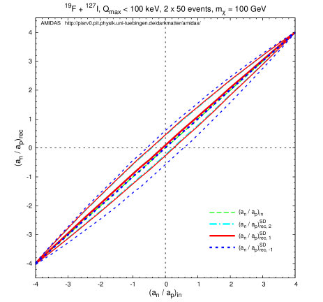
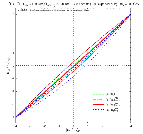
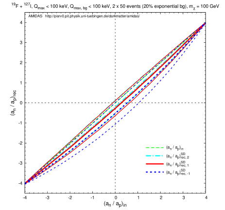
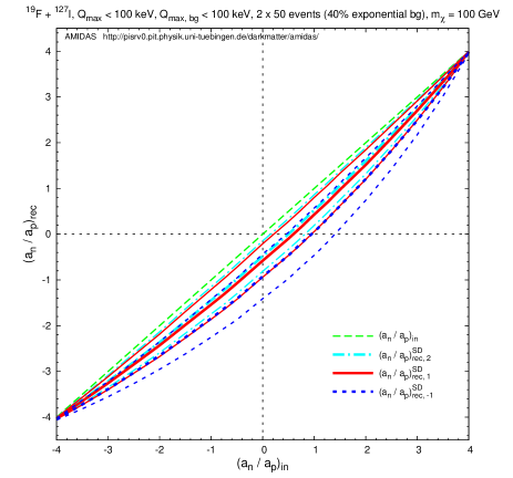
Figure 4: The reconstructed $a_{\rm n}/a_{\rm p}$ ratios estimated by Eq. (13) and the lower and upper bounds of their 1$\sigma$ statistical uncertainties estimated by Eq. (A18) with $n=-1$ (dashed blue), 1 (solid red), and 2 (dash–dotted cyan) as functions of the input $a_{\rm n}/a_{\rm p}$ ratio. Here the “$-$ (minus)” solution has been used (as the “inner” solution) [10]. The mass of incident WIMPs has been set as 100 GeV and each experiment contains 50 total events on average. The other parameters are as in Figs. 2. and 3.

It can be found here that, firstly, the statistical uncertainty on the reconstructed $a_{\rm n}/a_{\rm p}$ ratio with $n=2$ is a little bit smaller than the uncertainty on the ratio reconstructed with $n=1$, and both of them are much smaller than that reconstructed with $n=-1$. Secondly, due to the non–negligible background ratio in the analyzed data sets, the reconstructed $a_{\rm n}/a_{\rm p}$ ratios become underestimated; the larger the background ratio the larger this systematic deviation of the reconstructed $a_{\rm n}/a_{\rm p}$. However, for the same data sets, the larger the $n$ value (or, equivalently, the larger the moment of $f_{1}(v)$ used), the smaller this systematic deviation. This implies that the larger the background ratio, the more incompatibile between the $a_{\rm n}/a_{\rm p}$ ratios reconstructed with different $n$. This (in)compatibility could thus offer us a simple check for the purity/availability of our data sets.

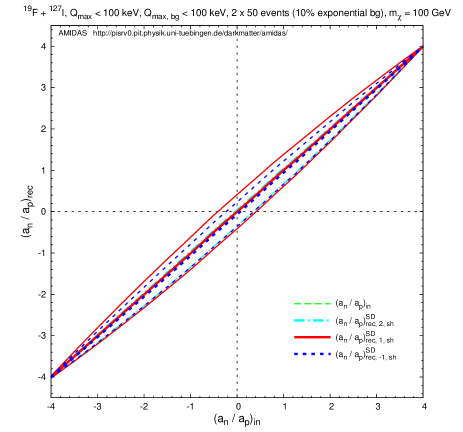
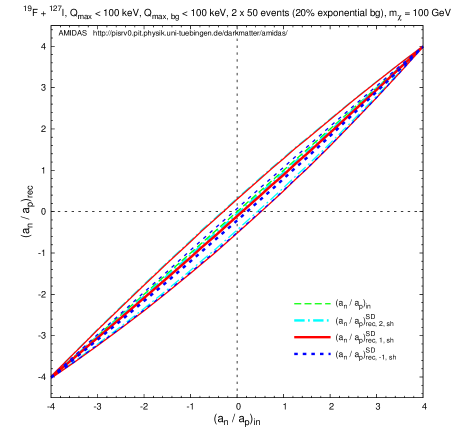
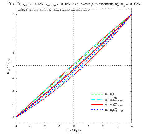
Figure 5: As in Figs. 4, except that we estimate $(a_{\rm n}/a_{\rm p})_{\pm,n}^{\rm SD}$ by Eq. (13) with the counting rates at the shifted points of the first $Q-$bin, $r_{(X,Y)}(Q_{s,1,(X,Y)})=r_{(X,Y),1}$.

In Figs. 5 I show the reconstructed $a_{\rm n}/a_{\rm p}$ ratios and the lower and upper bounds of their 1$\sigma$ statistical uncertainties estimated by Eqs. (13) and (A18) with the counting rates at the shifted points of the first $Q-$bin, $r_{(X,Y)}(Q_{s,1,(X,Y)})=r_{(X,Y),1}$, as functions of the input $a_{\rm n}/a_{\rm p}$ ratio. Different from the results shown in Figs. 4, the statistical uncertainty on the reconstructed $a_{\rm n}/a_{\rm p}$ ratio with $n=-1$ is a little bit smaller than those reconstructed with $n=2$ and $n=1$. But, the same as shown in Figs. 4, the larger the background ratio in the analyzed data sets, the more strongly the reconstructed $a_{\rm n}/a_{\rm p}$ ratios would be systematically underestimated, and the larger the $n$ value, the smaller this systematic deviation. However, the incompatibility between the $a_{\rm n}/a_{\rm p}$ ratios reconstructed with different $n$ is not so significant as shown in Figs. 4.

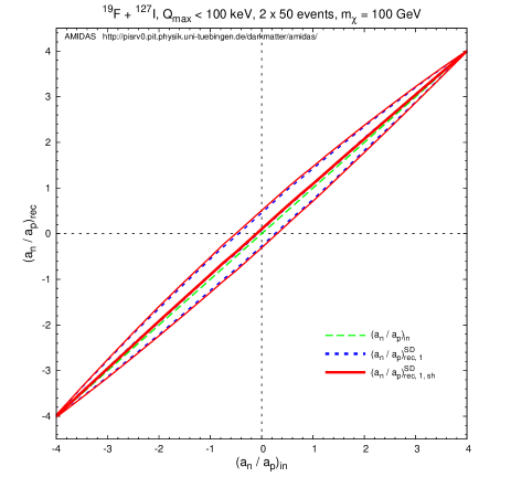
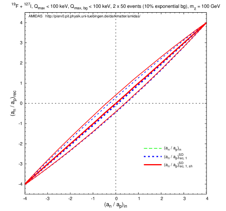
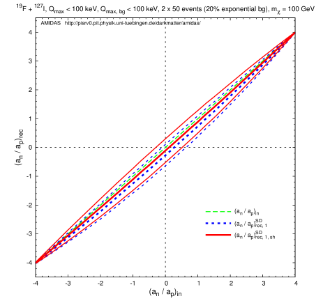
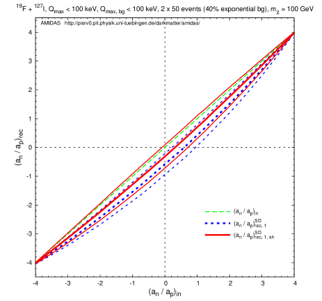
Figure 6: A comparison of the results shown in Figs. 4 estimated with $r_{(X,Y)}(Q_{{\rm min},(X,Y)}=0)$ (dashed blue) and those shown in Figs. 5 with $r_{(X,Y)}(Q_{s,1,(X,Y)})$ (solid red). Only the results estimated with $n=1$ are shown here.

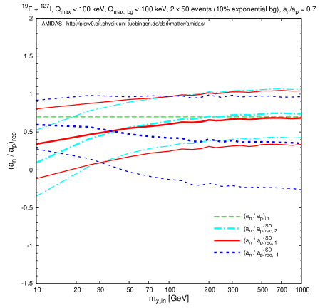
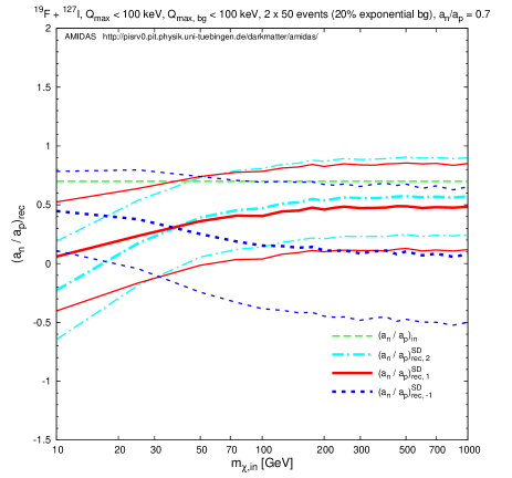
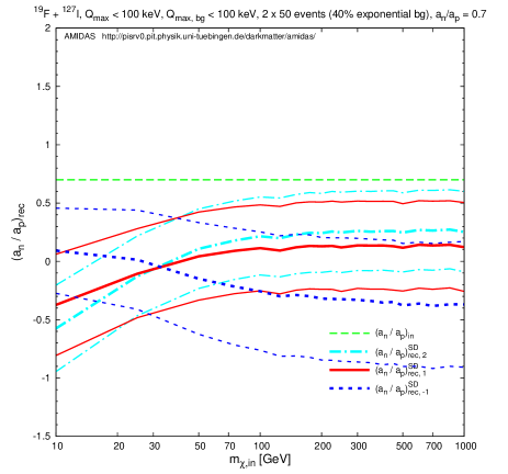
Figure 7: The reconstructed $a_{\rm n}/a_{\rm p}$ ratios estimated by Eq. (13) and the lower and upper bounds of their 1$\sigma$ statistical uncertainties estimated by Eq. (A18) with $n=-1$ (dashed blue), 1 (solid red), and 2 (dash–dotted cyan) as functions of the input WIMP mass $m_{\chi}$. The input $a_{\rm n}/a_{\rm p}$ ratio has been set as 0.7. The other parameters are as in Figs. 4.

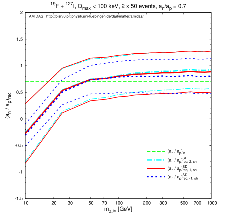
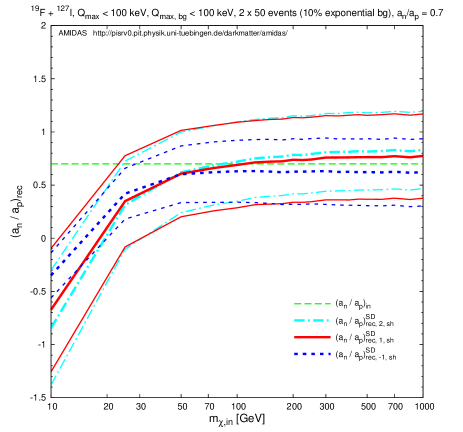
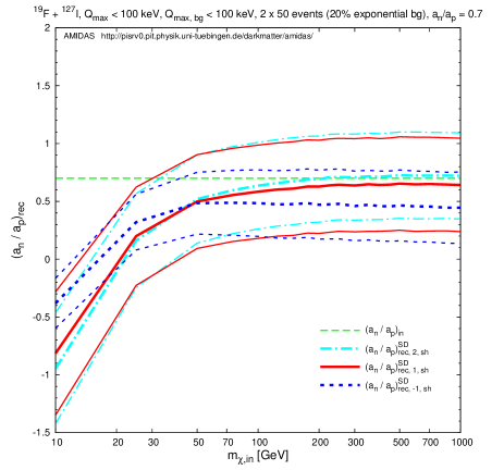
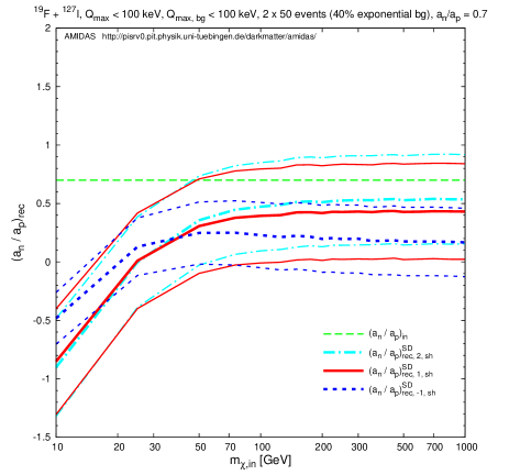
Figure 8: As in Figs. 7, except that we estimate $(a_{\rm n}/a_{\rm p})_{\pm,n}^{\rm SD}$ by Eq. (13) with the counting rates at the shifted points of the first $Q-$bin, $r_{(X,Y)}(Q_{s,1,(X,Y)})=r_{(X,Y),1}$.

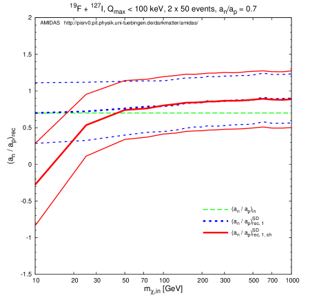
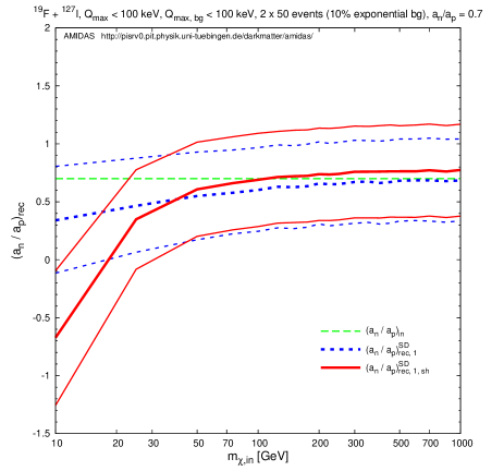
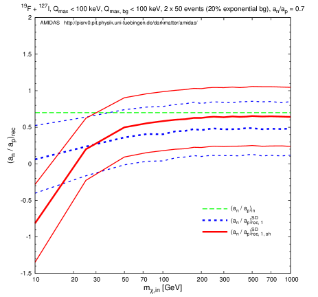
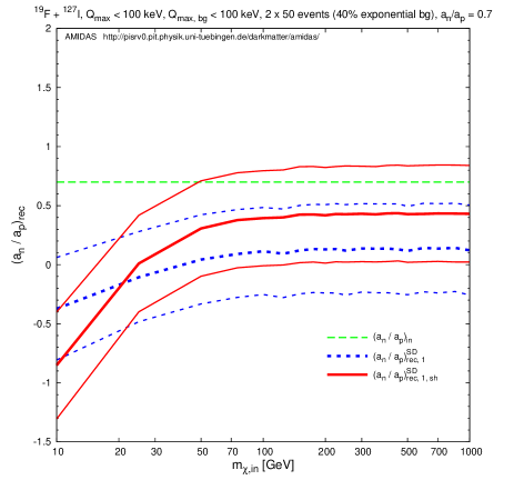
Figure 9: A comparison of the results shown in Figs. 7 estimated with $r_{(X,Y)}(Q_{{\rm min},(X,Y)}=0)$ (dashed blue) and those shown in Figs. 8 with $r_{(X,Y)}(Q_{s,1,(X,Y)})$ (solid red). Only the results estimated with $n=1$ are shown here.

As a comparison, I show the results shown in Figs. 4 estimated with $r_{(X,Y)}(Q_{{\rm min},(X,Y)}=0)$ (dashed blue) and those shown in Figs. 5 with $r_{(X,Y)}(Q_{s,1,(X,Y)})$ (solid red) together (only cases with $n=1$) in Figs. 6. It can be seen here clearly as well as from Figs. 4 and 5 that, because we set simply the experimental threshold energies to be negligible in our simulations, the statistical uncertainties on $a_{\rm n}/a_{\rm p}$ estimated with $r_{(X,Y)}(Q_{s,1,(X,Y)})$ are a little bit larger. However, as shown in Ref. [10], once threshold energies of analyzed data sets are non–negligible, the statistical uncertainties on $a_{\rm n}/a_{\rm p}$ estimated with $r_{(X,Y)}(Q_{s,1,(X,Y)})$ could be $\sim$ 16% smaller than those estimated with $r_{(X,Y)}(Q_{{\rm min},(X,Y)}=5~{}{\rm keV})$. Moreover, as shown here as well as in Figs. 4 and 5, for the cases with $r_{(X,Y)}(Q_{s,1,(X,Y)})$ the systematic deviations caused by residue background events are much smaller.

Quantitatively, Figs. 4 to 6 show that, with even $\sim$ 20% – 40% residue background events in the analyzed data sets, one could in principle still reconstruct the ratio between the SD WIMP couplings on neutrons and that on protons pretty well; for a WIMP mass $m_{\chi}=100$ GeV and $a_{\rm n}/a_{\rm p}=0.75$, by using Eq. (13) with $r_{(X,Y)}(Q_{{\rm min},(X,Y)}=0)$ (with $r_{(X,Y)}(Q_{s,1,(X,Y)})$) and $n=1$ to analyze data sets of a 10% (20%) background ratio, the systematic deviation could be $\>\raisebox{-3.01385pt}{$\stackrel{{\scriptstyle\textstyle<}}{{\sim}}$}\>-12\%$ ($\>\raisebox{-3.01385pt}{$\stackrel{{\scriptstyle\textstyle<}}{{\sim}}$}\>-14\%$) with an $\sim 55\%$ ($\sim 60\%$) statistical uncertainty.

The expression (13) for estimating the ratio between two SD WIMP–nucleon couplings is independent of the WIMP mass. However, as discussed in Sec. 3 and in Ref. [17] in more detail, an exponential–like residue background spectrum could cause an over–/underestimate of the reconstructed WIMP mass for light/heavy WIMPs. Hence, in order to check the WIMP–mass independence of the reconstructed $a_{\rm n}/a_{\rm p}$ ratio with non–negligible background events, in Figs. 7 and 8 I show the reconstructed results with $n=-1$ (dashed blue), 1 (solid red), and 2 (dash–dotted cyan) as functions of the input WIMP mass $m_{\chi}$. The input $a_{\rm n}/a_{\rm p}$ ratio has been set as 0.7.

It can be seen here that, for WIMP masses $m_{\chi}~{}\>\raisebox{-3.01385pt}{$\stackrel{{\scriptstyle\textstyle>}}{{\sim}}$}\>$ 50 GeV, except the statistical uncertainty estimated with $r_{(X,Y)}(Q_{{\rm min},(X,Y)})$ and $n=-1$ (dashed blue curves labeled as $(a_{\rm n}/a_{\rm p})_{\rm rec,~{}-1}^{\rm SD}$ in Figs. 7), the reconstructed $a_{\rm n}/a_{\rm p}$ ratios as well as their statistical uncertainties are indeed (almost) independent of the WIMP mass. However, as discussed above, the larger the background ratios in our data sets, the more strongly underestimated the reconstructed $a_{\rm n}/a_{\rm p}$ ratios for all input WIMP masses. And, as shown in Figs. 9, the $a_{\rm n}/a_{\rm p}$ ratios reconstructed with $r_{(X,Y)}(Q_{{\rm min},(X,Y)})$ (dashed blue) would be more strongly underestimated as those reconstructed with $r_{(X,Y)}(Q_{s,1,(X,Y)})$ (solid red). Nevertheless, with data sets of $\>\raisebox{-3.01385pt}{$\stackrel{{\scriptstyle\textstyle<}}{{\sim}}$}\>~{}20\%$ residue background events, the reconstructed 1$\sigma$ statistical uncertainty intervals could in principle always cover the input (true) $a_{\rm n}/a_{\rm p}$ ratios pretty well.

On the other hand, for WIMP masses $\>\raisebox{-3.01385pt}{$\stackrel{{\scriptstyle\textstyle<}}{{\sim}}$}\>~{}50$ GeV, interestingly, Figs. 7 show that the $a_{\rm n}/a_{\rm p}$ ratio reconstructed with $r_{(X,Y)}(Q_{{\rm min},(X,Y)})$ and $n=-1$ becomes the best result: with an $\>\raisebox{-3.01385pt}{$\stackrel{{\scriptstyle\textstyle<}}{{\sim}}$}\>~{}20\%$ background ratio the 1$\sigma$ statistical uncertainty interval could still cover the input (true) $a_{\rm n}/a_{\rm p}$ ratios well. In contrast, all other five reconstructed $a_{\rm n}/a_{\rm p}$ ratios shown in Figs. 7 and 8 are (strongly) underestimated.

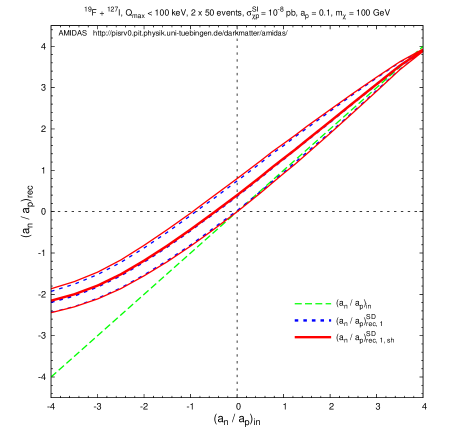
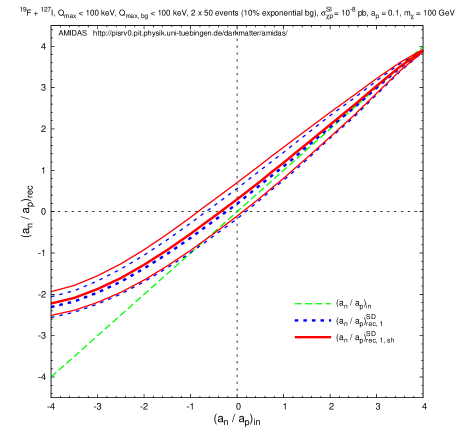
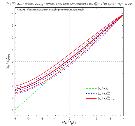
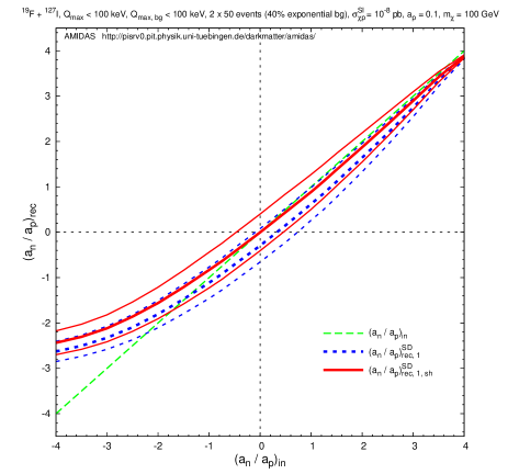
Figure 10: As in Figs. 6, except that the SI WIMP–nucleon cross section and the SD WIMP–proton coupling have been set as $\sigma_{\chi{\rm p}}^{\rm SI}=10^{-8}$ pb and $a_{\rm p}=0.1$, respectively.

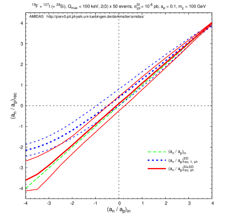
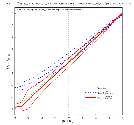
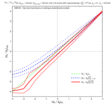
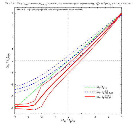
Figure 11: The reconstructed $a_{\rm n}/a_{\rm p}$ ratios estimated by Eqs. (13) (dashed blue, $n=1$) and (34) (solid red) and the lower and upper bounds of their 1$\sigma$ statistical uncertainties estimated by Eqs. (A18) and (A22) with $r_{(X,Y,Z)}(Q_{s,1,(X,Y,Z)})$ as functions of the input $a_{\rm n}/a_{\rm p}$ ratio. Besides ${}^{19}{\rm F}$ and ${}^{127}{\rm I}$, ${}^{28}{\rm Si}$ has been chosen as the third target for estimating $c_{{\rm p},(X,Y)}$ by Eqs. (35a) and (35b). The other parameters are as in Figs. 10.

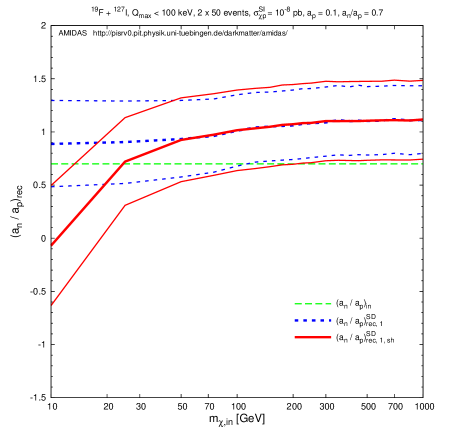
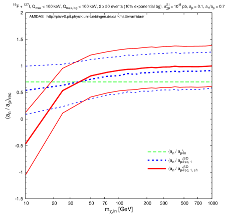
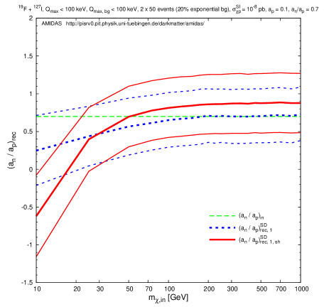
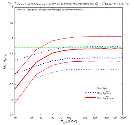
Figure 12: As in Figs. 9, except that the SI WIMP–nucleon cross section and the SD WIMP–proton coupling have been set as $\sigma_{\chi{\rm p}}^{\rm SI}=10^{-8}$ pb and $a_{\rm p}=0.1$, respectively.

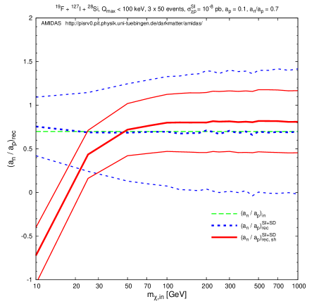
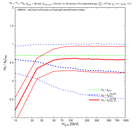
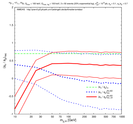
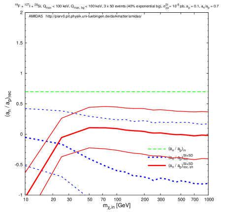
Figure 13: The reconstructed $a_{\rm n}/a_{\rm p}$ ratios estimated by Eq. (34) and the lower and upper bounds of their 1$\sigma$ statistical uncertainties estimated by Eq. (A22) with $r_{(X,Y,Z)}(Q_{{\rm min},(X,Y,Z)})$ (dashed blue) and with $r_{(X,Y,Z)}(Q_{s,1,(X,Y,Z)})$ (solid red) as functions of the input WIMP mass $m_{\chi}$. Besides ${}^{19}{\rm F}$ and ${}^{127}{\rm I}$, ${}^{28}{\rm Si}$ has been chosen as the third target for estimating $c_{{\rm p},(X,Y)}$ by Eqs. (35a) and (35b). The other parameters are as in Figs. 12.

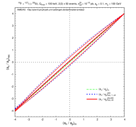
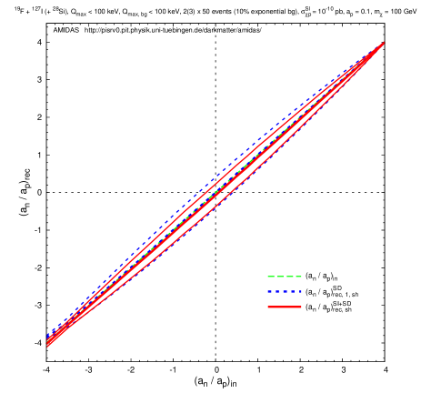
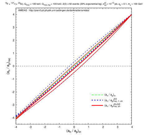
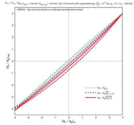
Figure 14: As in Figs. 11, except that the SI WIMP–nucleon cross section has been set as $\sigma_{\chi{\rm p}}^{\rm SI}=10^{-10}$ pb.

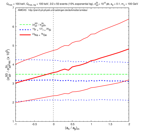
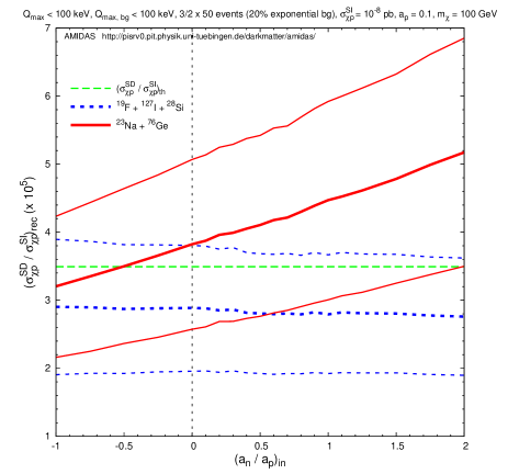
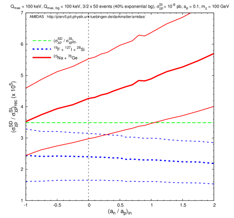
Figure 15: The reconstructed $\sigma_{\chi{\rm p}}^{\rm SD}/\sigma_{\chi{\rm p}}^{\rm SI}$ ratios and the lower and upper bounds of their 1$\sigma$ statistical uncertainties as functions of the input $a_{\rm n}/a_{\rm p}$ ratio. The dashed blue curves indicate the ratios estimated by Eq. (26) with $a_{\rm n}/a_{\rm p}$ estimated by Eq. (34) (not by Eq. (13)), whereas the solid red curves indicate the ratios estimated by Eq. (37). ${}^{76}{\rm Ge}$ has been chosen as the second target having only the SI interaction with WIMPs and combined with ${}^{23}{\rm Na}$ for using Eq. (37). Parameters are as in Figs. 11. Note that the input $a_{\rm n}/a_{\rm p}$ ratio ranges only between $-1$ and 2.

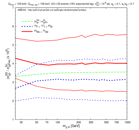
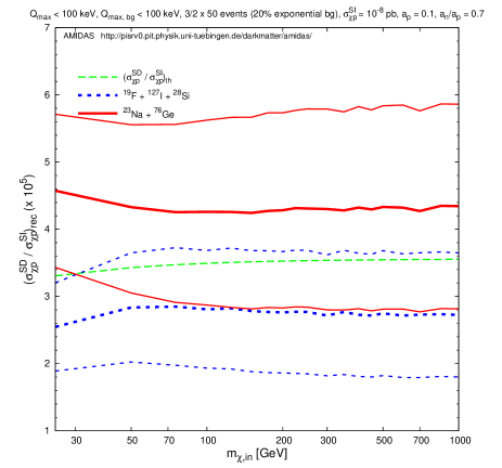
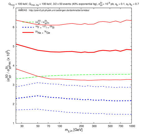
Figure 16: The reconstructed $\sigma_{\chi{\rm p}}^{\rm SD}/\sigma_{\chi{\rm p}}^{\rm SI}$ ratios and the lower and upper bounds of their 1$\sigma$ statistical uncertainties as functions of the input WIMP mass $m_{\chi}$. The input $a_{\rm n}/a_{\rm p}=0.7$, the other parameters and notations are as in Figs. 15. Note that the input WIMP mass starts from 25 GeV.

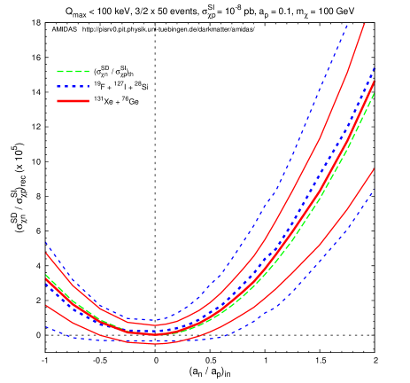
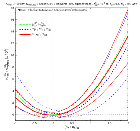
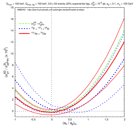
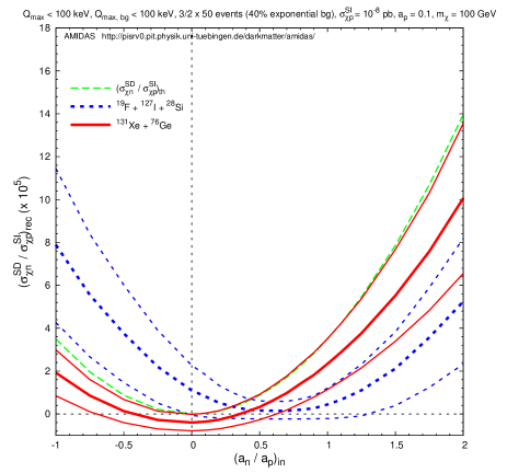
Figure 17: The reconstructed $\sigma_{\chi{\rm n}}^{\rm SD}/\sigma_{\chi{\rm p}}^{\rm SI}$ ratios and the lower and upper bounds of their 1$\sigma$ statistical uncertainties as functions of the input $a_{\rm n}/a_{\rm p}$ ratio. The dashed blue curves indicate the ratios estimated by Eq. (26) with $a_{\rm n}/a_{\rm p}$ estimated by Eq. (34), whereas the solid red curves indicate the ratios estimated by Eq. (37). ${}^{76}{\rm Ge}$ has been chosen as the second target having only the SI interaction with WIMPs and combined with ${}^{131}{\rm Xe}$ for using Eq. (37). Parameters are as in Figs. 15. Note that the input $a_{\rm n}/a_{\rm p}$ ratio ranges only between $-1$ and 2.

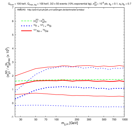
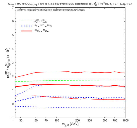
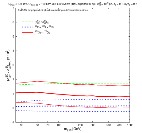
Figure 18: The reconstructed $\sigma_{\chi{\rm n}}^{\rm SD}/\sigma_{\chi{\rm p}}^{\rm SI}$ ratios and the lower and upper bounds of their 1$\sigma$ statistical uncertainties as functions of the input WIMP mass $m_{\chi}$. The input $a_{\rm n}/a_{\rm p}=0.7$, the other parameters and notations are as in Figs. 17. Note that the input WIMP mass starts from 25 GeV.

4.2 Reconstructed $(a_{\rm n}/a_{\rm p})_{\pm}^{\rm SI+SD}$

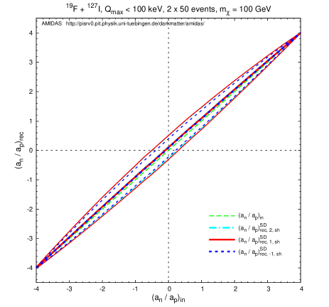
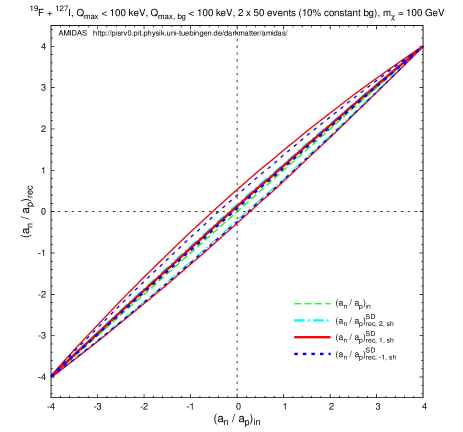
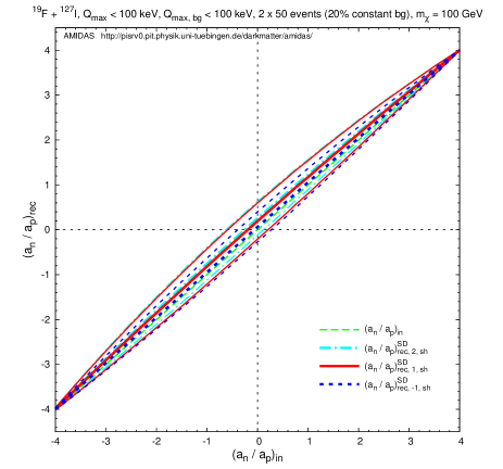
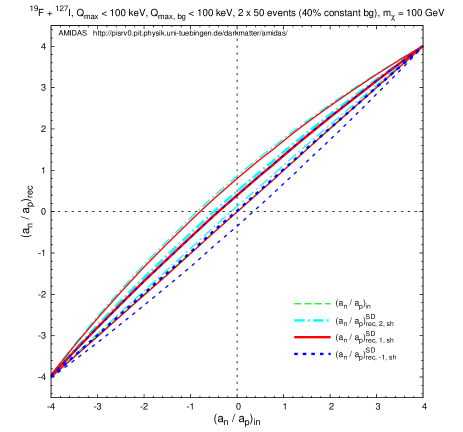
Figure 19: As in Figs. 5, except that the constant background spectrum has been used here.

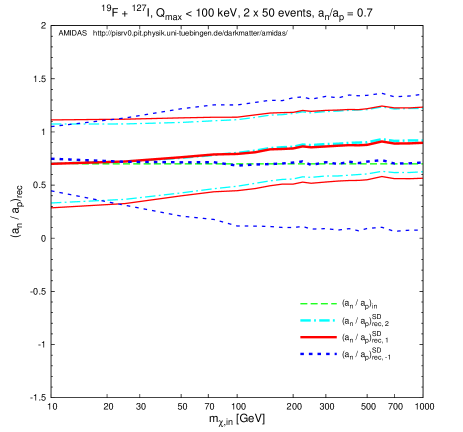
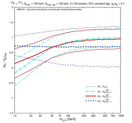
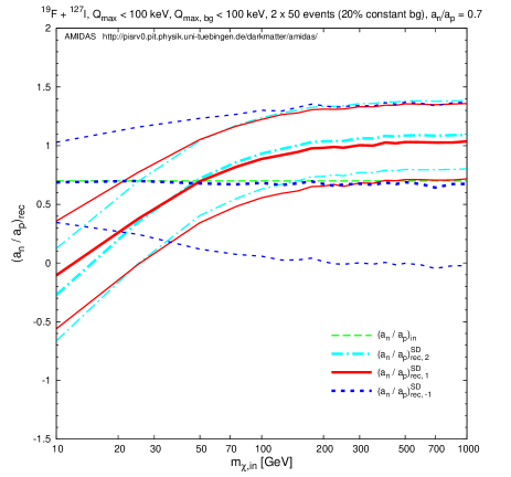
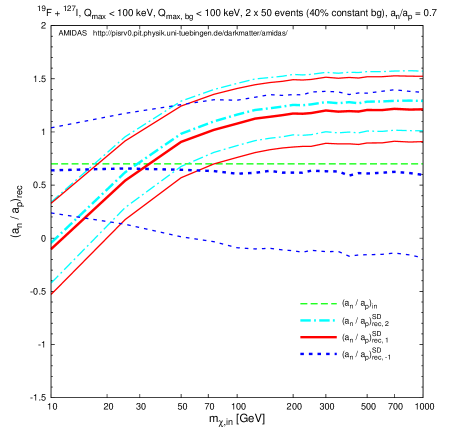
Figure 20: As in Figs. 7, except that the constant background spectrum has been used here.

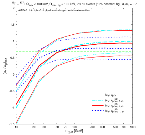
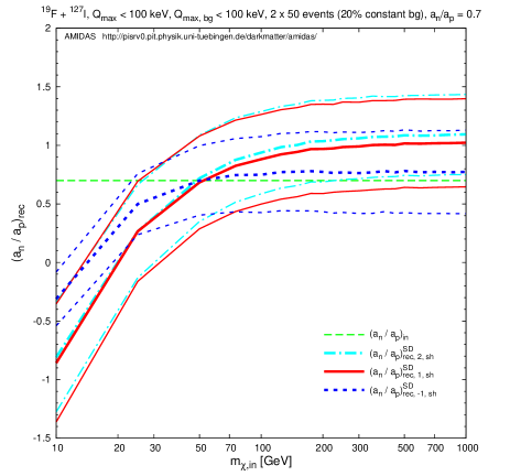
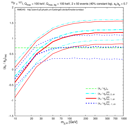
Figure 21: As in Figs. 8, except that the constant background spectrum has been used here.

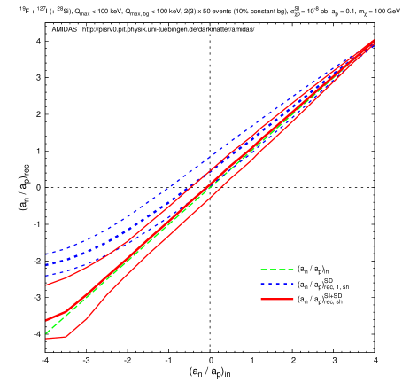
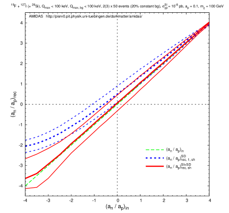
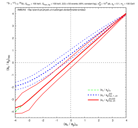
Figure 22: As in Figs. 11, except that the constant background spectrum has been used here.

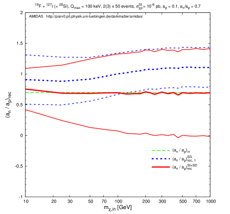
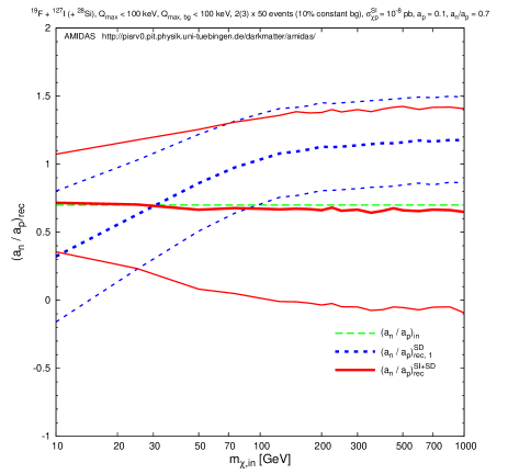
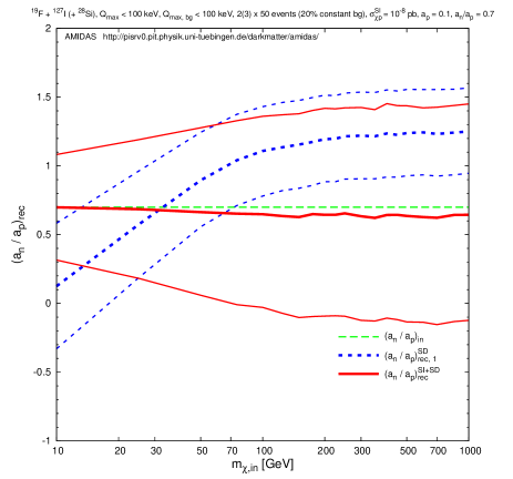
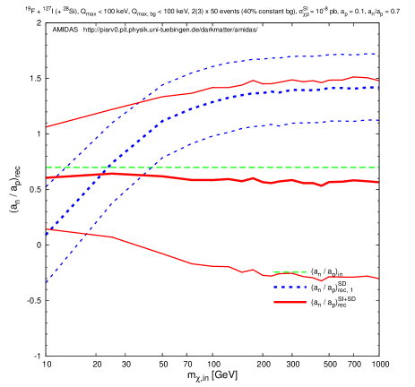
Figure 23: As in Figs. 12 and 13, except that the constant background spectrum has been used here. The dashed blue (solid red) curves indicate the reconstructed $a_{\rm n}/a_{\rm p}$ ratios estimated by Eq. (13) with $n=1$ (Eq. (34)) with $r_{(X,Y)}(Q_{{\rm min},(X,Y)})$ as functions of the input $a_{\rm n}/a_{\rm p}$ ratio.

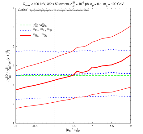
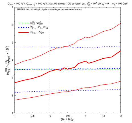
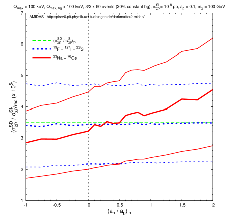
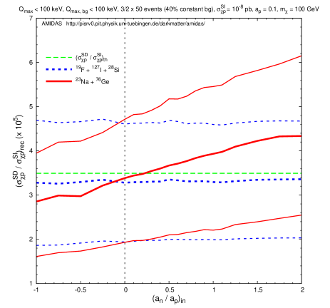
Figure 24: As in Figs. 15, except that the constant background spectrum has been used here.

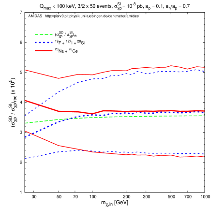
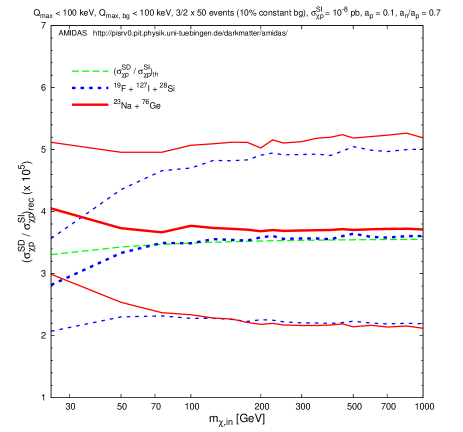
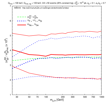
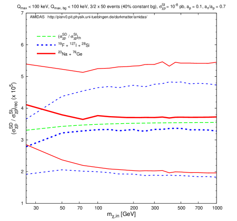
Figure 25: As in Figs. 16, except that the constant background spectrum has been used here.

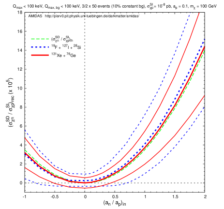
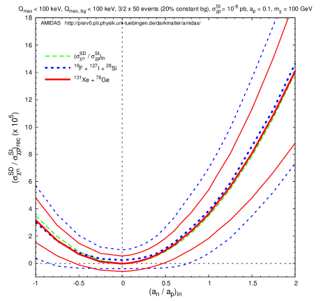
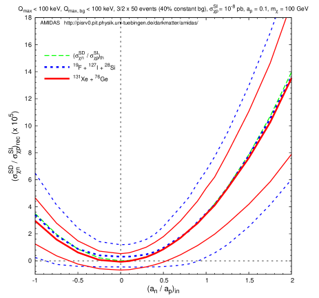
Figure 26: As in Figs. 17, except that the constant background spectrum has been used here.

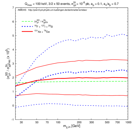
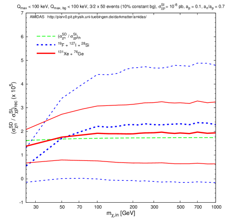
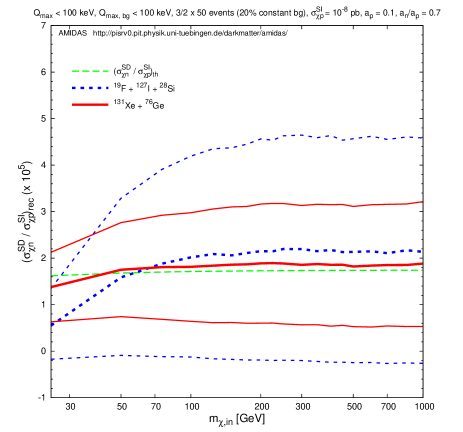
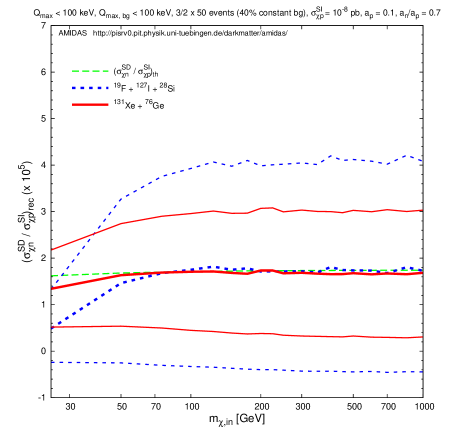
Figure 27: As in Figs. 18, except that the constant background spectrum has been used here.

In this and the next subsections I consider the case with a non–negligible SI WIMP–nucleus interaction. The input SI WIMP–nucleon cross section and the input SD WIMP–proton coupling have been set as $\sigma_{\chi{\rm p}}^{\rm SI}=10^{-8}$ pb and $a_{\rm p}=0.1$, respectively.

At first I show in Figs. 10 the reconstructed $a_{\rm n}/a_{\rm p}$ ratios estimated by Eq. (13) and the lower and upper bounds of their 1$\sigma$ statistical uncertainties estimated by Eq. (A18) with $r_{(X,Y)}(Q_{{\rm min},(X,Y)})$ (dashed blue) and with $r_{(X,Y)}(Q_{s,1,(X,Y)})$ (solid red) as functions of the input $a_{\rm n}/a_{\rm p}$ ratio together (only cases with $n=1$). Since for this simulation setup the SD WIMP–nucleus cross section doesn’t really dominate over the SI one, by using data sets with pure WIMP signals (no background events, top left frame), the reconstructed $a_{\rm n}/a_{\rm p}$ ratios are (strongly) overestimated, especially for the input $a_{\rm n}/a_{\rm p}\leq 0$. However, once some background events mix into our data sets, the reconstructed $a_{\rm n}/a_{\rm p}$ ratios become smaller (and even closer to the input (true) values, cf. Figs. 4 to 6). This seems to indicate that, with data sets of $\>\raisebox{-3.01385pt}{$\stackrel{{\scriptstyle\textstyle<}}{{\sim}}$}\>~{}40\%$ residue background events in the analyzed data sets, one could in principle reconstruct the ratio between two SD WIMP–nucleon couplings by simply assuming a dominant SD WIMP–nucleus interaction (even though this assumption is not correct) and using Eq. (13).

Nevertheless, once we consider both SI and SD WIMP interactions and thus use Eqs. (34) and (A22) to analyze the same data sets, as shown in Figs. 11, the $a_{\rm n}/a_{\rm p}$ ratios could be reconstructed (much) better with data sets of $\>\raisebox{-3.01385pt}{$\stackrel{{\scriptstyle\textstyle<}}{{\sim}}$}\>~{}20\%$ residue background events, even though the statistical uncertainties are pretty large for input $a_{\rm n}/a_{\rm p}\leq 0$. For a WIMP mass $m_{\chi}=100$ GeV and $a_{\rm n}/a_{\rm p}=0.75$, by using Eq. (34) with $r_{(X,Y,Z)}(Q_{s,1,(X,Y,Z)})$ to analyze data sets with a 10% background ratio, the systematic deviation could be $\sim-12\%$ with an $\sim 50\%$ statistical uncertainty. Moreover, with an increased background ratio, the (in)compatibility between the reconstructed $a_{\rm n}/a_{\rm p}$ ratios estimated by Eqs. (13) (dashed blue, $n=1$) and (34) (solid red) becomes larger. Hence, as mentioned in the previous subsection, one could/should compare results reconstructed under different assumptions, with both $r_{(X,Y,Z)}(Q_{{\rm min},(X,Y,Z)})$ and $r_{(X,Y,Z)}(Q_{s,1,(X,Y,Z)})$ and with different $n$ values, in order to check the purity of the analyzed data sets (as well as the dominance of the SI or the SD WIMP interaction [10]).

On the other hand, as done in the previous subsection, in order to check the WIMP–mass independence of the reconstructed results with non–negligible background events, I show the $a_{\rm n}/a_{\rm p}$ ratios estimated by Eq. (13) with $r_{(X,Y)}(Q_{{\rm min},(X,Y)})$ (dashed blue) and with $r_{(X,Y)}(Q_{s,1,(X,Y)})$ (solid red) as functions of the input WIMP mass $m_{\chi}$ together (only cases with $n=1$) in Figs. 12 as well as those estimated by Eq. (34) with $r_{(X,Y,Z)}(Q_{{\rm min},(X,Y,Z)})$ (dashed blue) and with $r_{(X,Y,Z)}(Q_{s,1,(X,Y,Z)})$ (solid red) as functions of the input WIMP mass $m_{\chi}$ in Figs. 13.

As shown earlier, for WIMP masses $m_{\chi}~{}\>\raisebox{-3.01385pt}{$\stackrel{{\scriptstyle\textstyle>}}{{\sim}}$}\>~{}50$ GeV, the reconstructed $a_{\rm n}/a_{\rm p}$ ratios are indeed (almost) independent of $m_{\chi}$. And, with data sets of $\>\raisebox{-3.01385pt}{$\stackrel{{\scriptstyle\textstyle<}}{{\sim}}$}\>~{}20\%$ background ratios, using Eq. (34) (solid red in Figs. 13) and estimating with $r_{(X,Y,Z)}(Q_{s,1,(X,Y,Z)})$ could offer the best reconstructed $a_{\rm n}/a_{\rm p}$ ratios. Meanwhile, for WIMP masses $m_{\chi}~{}\>\raisebox{-3.01385pt}{$\stackrel{{\scriptstyle\textstyle<}}{{\sim}}$}\>~{}50$ GeV, Figs. 13 show also that the $a_{\rm n}/a_{\rm p}$ ratios reconstructed by Eq. (34) with $r_{(X,Y,Z)}(Q_{{\rm min},(X,Y,Z)})$ could be the best results (with however a pretty large statistical uncertainty): for a WIMP mass $m_{\chi}=25$ GeV and an input $a_{\rm n}/a_{\rm p}=0.7$, by using Eq. (34) with $r_{(X,Y,Z)}(Q_{{\rm min},(X,Y,Z)})$ to analyze data sets of a 10% background ratio, the systematic deviation could be $\sim-25\%$ with an $\sim 88\%$ statistical uncertainty.

Furthermore, in Figs. 14 we reduce the SI WIMP–nucleon cross section two orders of magnitude smaller: $\sigma_{\chi{\rm p}}^{\rm SI}=10^{-10}$ pb. It can be found here that, although the $a_{\rm n}/a_{\rm p}$ ratios reconstructed by Eqs. (13) (dashed blue, $n=1$) and (34) (solid red) with $r_{(X,Y,Z)}(Q_{s,1,(X,Y,Z)})$ match much better than those shown in Figs. 11, with an increased background ratio the $a_{\rm n}/a_{\rm p}$ ratios could be a bit more strongly underestimated by using Eq. (34). Nevertheless, Figs. 11, Figs. 13, and Figs. 14 show that, it doesn’t matter whether the SD WIMP–nucleus interaction really dominates over the SI one or not, by using Eq. (34) one could in principle always reconstruct the ratio of the SD WIMP coupling on neutrons to that on protons with data sets of $\>\raisebox{-3.01385pt}{$\stackrel{{\scriptstyle\textstyle<}}{{\sim}}$}\>~{}20\%$ residue background events pretty well. But, the larger the relative strength between the SD WIMP–nucleus interaction to the SI one, the smaller the systematic deviations as well as the statistical uncertainties. For $\sigma_{\chi{\rm p}}^{\rm SI}=10^{-10}$ pb with a WIMP mass $m_{\chi}=100$ GeV and $a_{\rm n}/a_{\rm p}=0.75$, by using data sets of a 10% background ratio, the systematic deviation could be $\sim-10\%$ with an $\sim 43\%$ statistical uncertainty.

4.3 Reconstructed $\sigma_{\chi({\rm p,n})}^{\rm SD}/\sigma_{\chi{\rm p}}^{\rm SI}$

In Figs. 15 and 16 I show the reconstructed $\sigma_{\chi{\rm p}}^{\rm SD}/\sigma_{\chi{\rm p}}^{\rm SI}$ ratios and the lower and upper bounds of their 1$\sigma$ statistical uncertainties as functions of the input $a_{\rm n}/a_{\rm p}$ ratio as well as of the input WIMP mass $m_{\chi}$, respectively. The dashed blue curves indicate the ratios estimated by Eq. (26) with $a_{\rm n}/a_{\rm p}$ estimated by Eq. (34) (not by Eq. (13)), whereas the solid red curves indicate the ratios estimated by Eq. (37). ${}^{76}{\rm Ge}$ has been chosen as the second target having only the SI interaction with WIMPs and combined with ${}^{23}{\rm Na}$ for using Eq. (37).

It can be seen here that, interestingly, while the $\sigma_{\chi{\rm p}}^{\rm SD}/\sigma_{\chi{\rm p}}^{\rm SI}$ ratios reconstructed with $\rm F+I+Si$ targets become as usual more and more strongly underestimated with an increased background ratio, those reconstructed with $\rm Na+Ge$ targets become in contrast more and more strongly overestimated. Nevertheless, for WIMP masses $m_{\chi}~{}\>\raisebox{-3.01385pt}{$\stackrel{{\scriptstyle\textstyle>}}{{\sim}}$}\>~{}25$ GeV, with $\>\raisebox{-3.01385pt}{$\stackrel{{\scriptstyle\textstyle<}}{{\sim}}$}\>~{}20\%$ residue background events, the overlap of the 1$\sigma$ statistical uncertainty intervals estimated by two target combinations could cover the input (true) $\sigma_{\chi{\rm p}}^{\rm SD}/\sigma_{\chi{\rm p}}^{\rm SI}$ ratio well. For a WIMP mass $m_{\chi}=100$ GeV and $a_{\rm n}/a_{\rm p}=0.7$ (the theoretical value of $\sigma_{\chi{\rm p}}^{\rm SD}/\sigma_{\chi{\rm p}}^{\rm SI}=3.49\times 10^{5}$), by using $\rm F+I+Si$ ($\rm Na+Ge$) targets with data sets of a 20% background ratio, one could in principle reconstruct the $\sigma_{\chi{\rm p}}^{\rm SD}/\sigma_{\chi{\rm p}}^{\rm SI}$ ratio with an $\sim-20\%$ ($\sim+21\%$) systematic deviation and an $\sim 31\%$ ($\sim 32\%$) statistical uncertainty.

On the other hand, in Figs. 17 and 18 I show the reconstructed $\sigma_{\chi{\rm n}}^{\rm SD}/\sigma_{\chi{\rm p}}^{\rm SI}$ ratios and the lower and upper bounds of their 1$\sigma$ statistical uncertainties as functions of the input $a_{\rm n}/a_{\rm p}$ ratio as well as of the input WIMP mass $m_{\chi}$, respectively. The dashed blue curves indicate the ratios estimated by Eq. (26) with $a_{\rm n}/a_{\rm p}$ estimated by Eq. (34), whereas the solid red curves indicate the ratios estimated by Eq. (37). ${}^{76}{\rm Ge}$ has been chosen as the second target having only the SI interaction with WIMPs and combined with ${}^{131}{\rm Xe}$ for using Eq. (37).

It can be found here that, more interestingly, while the $\sigma_{\chi{\rm n}}^{\rm SD}/\sigma_{\chi{\rm p}}^{\rm SI}$ ratios reconstructed with $\rm F+I+Si$ targets become more and more strongly underestimated with an increased background ratio for all input $a_{\rm n}/a_{\rm p}$ values, those reconstructed with $\rm Xe+Ge$ targets become more and more strongly underestimated for $a_{\rm n}/a_{\rm p}~{}\>\raisebox{-3.01385pt}{$\stackrel{{\scriptstyle\textstyle>}}{{\sim}}$}\>~{}0$ and more and more strongly overestimated for $a_{\rm n}/a_{\rm p}~{}\>\raisebox{-3.01385pt}{$\stackrel{{\scriptstyle\textstyle<}}{{\sim}}$}\>~{}0$. Nevertheless, for WIMP masses $m_{\chi}~{}\>\raisebox{-3.01385pt}{$\stackrel{{\scriptstyle\textstyle>}}{{\sim}}$}\>~{}25$ GeV, with $\>\raisebox{-3.01385pt}{$\stackrel{{\scriptstyle\textstyle<}}{{\sim}}$}\>~{}20\%$ residue background events, the (overlap of the) 1$\sigma$ statistical uncertainty intervals estimated by two target combinations could cover the input (true) $\sigma_{\chi{\rm n}}^{\rm SD}/\sigma_{\chi{\rm p}}^{\rm SI}$ ratio well. For a WIMP mass $m_{\chi}=100$ GeV and $a_{\rm n}/a_{\rm p}=0.7$ (the theoretical value of $\sigma_{\chi{\rm n}}^{\rm SD}/\sigma_{\chi{\rm p}}^{\rm SI}=1.71\times 10^{5}$), by using $\rm F+I+Si$ ($\rm Xe+Ge$) targets with data sets of a 10% background ratio, one could in principle reconstruct the $\sigma_{\chi{\rm p}}^{\rm SD}/\sigma_{\chi{\rm p}}^{\rm SI}$ ratio with an $\sim-32\%$ ($\sim-3.2\%$) systematic deviation and an $\sim 120\%$ ($\sim 62\%$) statistical uncertainty.

5 Results of the reconstructed ratios of WIMP–nucleon couplings/cross sections II: with constant background spectra

In this section I show simulation results with residue background events generated by the constant spectrum given in Eq. (45) and compare them with those shown in the previous section. Some general rules about the effects of different background sources will also be discussed.

5.1 Reconstructed $(a_{\rm n}/a_{\rm p})_{\pm,n}^{\rm SD}$

As in the previous section, I consider at first the case of a dominant SD WIMP–nucleus interaction.

In Figs. 19 I show the reconstructed $a_{\rm n}/a_{\rm p}$ ratios and the lower and upper bounds of their 1$\sigma$ statistical uncertainties estimated by Eqs. (13) and (A18) with $n=-1$ (dashed blue), 1 (solid red), and 2 (dash–dotted cyan) as functions of the input $a_{\rm n}/a_{\rm p}$ ratio. Note that only results with the counting rates at the shifted points of the first $Q-$bin, $r_{(X,Y)}(Q_{s,1,(X,Y)})$, are shown here, because their systematic deviations due to the non–negligible background events as well as their statistical uncertainties (for non–zero experimental threshold energies) are (much) smaller.

It can be found here that, firstly, in contrast to the results shown in Figs. 4 to 6, the $a_{\rm n}/a_{\rm p}$ ratios reconstructed with $n=1$ (solid red) and 2 (dash–dotted cyan) are now overestimated. This should be caused by the background contribution to high energy ranges. Remind that, as shown in Figs. 2 and 3, while an exponential(–like) background spectrum contributes (almost) only/mainly to low energy ranges, a constant/(approximately) flat one contributes mainly to high energy ranges. This indicates in turn that, while the reconstructed $a_{\rm n}/a_{\rm p}$ ratio would be underestimated by using data sets with residue background events existing mostly in low energy ranges, e.g., electronic noise or incompletely charged surface events, the $a_{\rm n}/a_{\rm p}$ ratio would be overestimated by using data sets with backgrounds relatively mainly in high energy ranges, e.g., cosmic rays and cosmic–ray induced $\gamma$-rays with energies of $\cal O$(100) keV.

However, interestingly and importantly, the $a_{\rm n}/a_{\rm p}$ ratio reconstructed with $n=-1$ (dashed blue) in Figs. 19 is almost not affected by the constant background spectrum! The reason can be understood as follows. The $(a_{\rm n}/a_{\rm p})_{-,-1,{\rm sh}}^{\rm SD}$ ratio has been estimated with ${\cal R}_{J,-1,(X,Y)}$ given in Eq. (21) and is in fact a function of only $r_{(X,Y)}(Q_{s,1,(X,Y)})$. Since the constant background spectra contribute only (very) small amounts to the lowest energy ranges (see Figs. 3), $r_{(X,Y)}(Q_{s,1,(X,Y)})$ estimated by using events recorded in the first $Q-$bins would not change or only very slightly, and in turn also the reconstructed $a_{\rm n}/a_{\rm p}$ ratio.

In Figs. 20 and 21, I show the reconstructed $a_{\rm n}/a_{\rm p}$ ratios as functions of the input WIMP mass. Both of them show that, while the $a_{\rm n}/a_{\rm p}$ ratios reconstructed with $n=1$ (solid red) and 2 (dash–dotted cyan) are more and more strongly overestimated with an increased background ratio, the ratios reconstructed with $n=-1$ (dashed blue) just become a little bit smaller ($\sim$ 15% smaller for a background ratio of 40% and an input WIMP mass of 1 TeV, compared to the results with no background events) and the statistical uncertainties also grow only slightly ($\>\raisebox{-3.01385pt}{$\stackrel{{\scriptstyle\textstyle<}}{{\sim}}$}\>~{}45\%$ larger).

5.2 Reconstructed $(a_{\rm n}/a_{\rm p})_{\pm}^{\rm SI+SD}$

In this subsection I consider the reconstruction of the $a_{\rm n}/a_{\rm p}$ ratio with a non–zero SI WIMP–nucleus cross section.

As shown in the previous subsection, Figs. 22 and 23 show that, while with an increased background ratio the $a_{\rm n}/a_{\rm p}$ ratios reconstructed by Eq. (13) (dashed blue, with $n=1$ and $r_{(X,Y)}(Q_{{\rm min},(X,Y)}=0)$ or $r_{(X,Y)}(Q_{s,1,(X,Y)})$) are more and more strongly overestimated caused by contributions of the constant background spectrum to high energy ranges, those reconstructed by Eq. (34) (solid red) just become a little bit smaller ($\sim$ 9% smaller for a background ratio of 40% and an input WIMP mass of 100 GeV, compared to the results with no background events) and the statistical uncertainties also grow only slightly ($\sim$ 34% larger).

This is simply because that $(a_{\rm n}/a_{\rm p})_{-}^{\rm SI+SD}$ given in Eq. (34) depends only on $c_{{\rm p},(X,Y)}$, which are in turn just the functions of $r_{(X,Y,Z)}(Q_{{\rm min},(X,Y,Z)})$ or $r_{(X,Y,Z)}(Q_{s,1,(X,Y,Z)})$ and can be estimated by using events in the lowest energy ranges. Hence, once residue background events exist regularly between the experimental minimal and maximal cut–off energies or (even better) (mostly) in high energy ranges, one can in principle estimate $r_{(X,Y,Z)}(Q_{{\rm min},(X,Y,Z)})$ and $r_{(X,Y,Z)}(Q_{s,1,(X,Y,Z)})$ as well as the ratio between two SD WIMP–nucleon couplings (pretty) precisely by using Eq. (34) without worrying about the non–negligible backgrounds.

5.3 Reconstructed $\sigma_{\chi({\rm p,n})}^{\rm SD}/\sigma_{\chi{\rm p}}^{\rm SI}$

Finally, we check the reconstruction of the ratios between the SD and SI WIMP–proton(neutron) cross sections by using Eqs. (26) and (37) with the constant background spectrum.

In Figs. 24 and 25 we can find that, as observed in Sec. 4.3, while the $\sigma_{\chi{\rm p}}^{\rm SD}/\sigma_{\chi{\rm p}}^{\rm SI}$ ratios reconstructed with $\rm F+I+Si$ targets by Eq. (26) with $a_{\rm n}/a_{\rm p}$ reconstructed by Eq. (34) (dashed blue) become more and more strongly underestimated with an increased background ratio, those reconstructed with $\rm Na+Ge$ targets by Eq. (37) (solid red) become more and more strongly overestimated. Meanwhile, Figs. 26 and 27 show that, while the $\sigma_{\chi{\rm n}}^{\rm SD}/\sigma_{\chi{\rm p}}^{\rm SI}$ ratios reconstructed with $\rm F+I+Si$ targets (dashed blue) become more and more strongly underestimated with an increased background ratio for all $a_{\rm n}/a_{\rm p}$ values, those reconstructed with $\rm Xe+Ge$ targets (solid red) become more and more strongly underestimated for $a_{\rm n}/a_{\rm p}~{}\>\raisebox{-3.01385pt}{$\stackrel{{\scriptstyle\textstyle>}}{{\sim}}$}\>~{}0$ and more and more strongly overestimated for $a_{\rm n}/a_{\rm p}~{}\>\raisebox{-3.01385pt}{$\stackrel{{\scriptstyle\textstyle<}}{{\sim}}$}\>~{}0$.

However, the shifts caused by events with the constant background spectrum are much smaller than those caused with the exponential one. Quantitatively, for an input WIMP mass of 100 GeV, an input SI WIMP–nucleon cross section of $10^{-8}$ pb, an input SD WIMP–proton coupling $a_{\rm p}=0.1$, and an input $a_{\rm n}/a_{\rm p}=0.7$, by using 2 (3) data sets of a 40% background ratio, the $\sigma_{\chi{\rm p}}^{\rm SD}/\sigma_{\chi{\rm p}}^{\rm SI}$ ratios would be reconstructed 4% larger (7% smaller) with $<$ 20% larger statistical uncertainties, whereas the $\sigma_{\chi{\rm n}}^{\rm SD}/\sigma_{\chi{\rm p}}^{\rm SI}$ ratios would be reconstructed 14% (30%) smaller with $\sim$ 30% larger statistical uncertainties, compared to the results with no background events.

These results indicate that, once residue background events exist regularly between the experimental minimal and maximal cut–off energies or (mostly) in high energy ranges and one can therefore in principle estimate $r_{(X,Y,Z)}(Q_{{\rm min},(X,Y,Z)})$ and $r_{(X,Y,Z)}(Q_{s,1,(X,Y,Z)})$ (pretty) well, the ratios between the SD and SI WIMP–nucleon cross sections could then be estimated (pretty) precisely without worrying about the non–negligible backgrounds.

6 Summary and conclusions

In this paper I reexamine the model–independent data analysis methods introduced in Refs. [9, 10] for the determinations of ratios between different WIMP–nucleon couplings/cross sections from data (measured recoil energies) of direct Dark Matter detection experiments directly by taking into account a fraction of residue background events, which pass all discrimination criteria and then mix with other real WIMP–induced events in the analyzed data sets. These methods require neither prior knowledge about the WIMP scattering and different possible background spectra nor about the WIMP mass; the unique needed information is the recoil energies recorded in two (or more) direct detection experiments.

I considered at first the case of a dominant SD WIMP–nucleus interaction. Our simulations show that, due to the contribution of non–negligible residue background events in the analyzed data sets to low/high energy ranges, the reconstructed $a_{\rm n}/a_{\rm p}$ ratios would be under-/overestimated; the larger the background ratio the larger these systematic deviations of the reconstructed $a_{\rm n}/a_{\rm p}$. But, by estimating the counting rates at the shifted points, instead of at the experimental minimal cut–off energies, one could (strongly) alleviate these systematic deviations as well as reduce the statistical uncertainties (with non–negligible experimental threshold energies). By using data sets of $\sim$ 20% – 40% residue background events, the ratio between the SD WIMP couplings on neutrons and on protons could in principle still be reconstructed pretty well: for a WIMP mass $m_{\chi}=100$ GeV and $a_{\rm n}/a_{\rm p}=0.75$, with data sets of a 10% (20%) background ratio, the systematic deviation could be $\>\raisebox{-3.01385pt}{$\stackrel{{\scriptstyle\textstyle<}}{{\sim}}$}\>-12\%$ ($\>\raisebox{-3.01385pt}{$\stackrel{{\scriptstyle\textstyle<}}{{\sim}}$}\>-14\%$) with an $\sim 55\%$ ($\sim 60\%$) statistical uncertainty.

Then I turned to consider the general combination of the SD WIMP–nucleus interaction with a non–negligible SI one. Our simulations show that, by combining three (two spin–sensitive) target nuclei, our method can be used to reconstruct the ratio of the SD WIMP coupling on neutrons to that on protons with data sets of $\>\raisebox{-3.01385pt}{$\stackrel{{\scriptstyle\textstyle<}}{{\sim}}$}\>~{}20\%$ residue background events. And, more importantly, it doesn’t matter whether the SD WIMP–nucleus cross section really dominates over the SI one or not. But, the larger the relative strength between the SD WIMP–nucleus interaction to the SI one, the smaller the systematic deviations as well as the statistical uncertainties.

I considered also the reconstruction of the ratios between the SD and SI WIMP–nucleon cross sections. For WIMP masses $m_{\chi}~{}\>\raisebox{-3.01385pt}{$\stackrel{{\scriptstyle\textstyle>}}{{\sim}}$}\>~{}25$ GeV, by using either the reconstructed $a_{\rm n}/a_{\rm p}$ ratio or a combination of a spin–sensitive nucleus with an only SI–sensitive one with data sets of $\>\raisebox{-3.01385pt}{$\stackrel{{\scriptstyle\textstyle<}}{{\sim}}$}\>~{}20\%$ background ratios, while the $\sigma_{\chi{\rm p}}^{\rm SD}/\sigma_{\chi{\rm p}}^{\rm SI}$ ratio could be reconstructed with a $\sim$ 30% statistical uncertainty, one could (only) estimate the order of magnitude of the $\sigma_{\chi{\rm n}}^{\rm SD}/\sigma_{\chi{\rm p}}^{\rm SI}$ ratio (because of an $\sim$ 120% statistical uncertainty).

Moreover, our simulations show also the WIMP–mass independence of the reconstructed $a_{\rm n}/a_{\rm p}$ ratios with non–negligible background events, especially for WIMP masses $m_{\chi}~{}\>\raisebox{-3.01385pt}{$\stackrel{{\scriptstyle\textstyle>}}{{\sim}}$}\>$ 50 GeV. For WIMP masses $\>\raisebox{-3.01385pt}{$\stackrel{{\scriptstyle\textstyle<}}{{\sim}}$}\>~{}50$ GeV, the $a_{\rm n}/a_{\rm p}$ ratios could be (strongly) underestimated, even with zero background events. However, this underestimate could be alleviated/corrected by decrease the experimental minimal cut–off energies of the analyzed date sets (to be negligible). Then, with data sets of $\>\raisebox{-3.01385pt}{$\stackrel{{\scriptstyle\textstyle<}}{{\sim}}$}\>~{}20\%$ residue background events, one could still reconstruct the $a_{\rm n}/a_{\rm p}$ ratios pretty well, by either assuming a dominant SD WIMP interaction or using the general combination of the SI and SD cross sections. But, the statistical uncertainty could be pretty large, once the SD WIMP–nucleus interaction doesn’t dominate over the SI one.

Furthermore, it has also been found that, firstly, by taking different assumptions about the relative strength between the SI and SD WIMP–nucleus interactions, and/or using different moments of the one–dimensional WIMP velocity distribution function, at either the experimental minimal cut–off energies or the shifted energy points, there would be an (in)compatibility between different reconstructed $a_{\rm n}/a_{\rm p}$ ratios; with an increased background ratio, the incompatibility between the reconstructed results would become larger. Hence, this (in)compatibility could allow us to check the purity/availability of the analyzed data sets (as well as the dominance of the SI or SD WIMP interaction).

Secondly and more importantly, our simulations with a constant background spectrum indicate that, once residue background events exist regularly between the experimental minimal and maximal cut–off energies or (even better) (mostly) in high energy ranges, one could in principle estimate the counting rates of the recoil spectrum of only WIMP–induced events at the experimental threshold energies (pretty) precisely. Then the ratio between two SD WIMP–nucleon couplings as well as the ratios between the SD and SI WIMP–nucleon cross sections could be estimated (pretty) precisely without worrying about the non–negligible backgrounds.

In summary, as the forth part of the study of the effects of residue background events in direct Dark Matter detection experiments, we considered the determinations of ratios between different WIMP–nucleon couplings/cross sections. Our results show that, with currently running and projected experiments using detectors with $10^{-9}$ to $10^{-11}$ pb sensitivities [32, 14, 33, 34] and $<10^{-6}$ background rejection ability [13, 15, 16, 12], once two or more experiments with different spin–sensitive target nuclei could accumulate a few tens events (in one experiment), we could in principle already estimate the relative strengths of couplings/cross sections of Dark Matter particles on ordinary matter with a reasonable precession, even though there could be some background events mixed in our data sets for analyses. Moreover, although two forms for background spectrum considered in this work is rather naive, the nuclear form factors for the SD WIMP interaction with different target nuclei are also more complicated as the simple thin–shell form used in our simulations, and the relative signs of the (ratios of the) expected/measured proton/neutron group spins of the used target nuclei could also change the reconstructed results (to be larger or smaller, underestimated or overestimated), one should be able to extend our observations/discussions to predict the effects of possible background events in their own experiments. Hopefully, this will not only encourage our experimental colleagues to present their (future) results in the parameter space of Dark Matter particles, but also help them to check the purity of their data sets, to understand (residue) background events in their experiments, as well as to improve their background discrimination techniques.

Acknowledgments

The author would like to thank the Physikalisches Institut der Universität Tübingen for the technical support of the computational work demonstrated in this article. This work was partially supported by the National Science Council of R.O.C. under contract no. NSC-99-2811-M-006-031 as well as by the LHC Physics Focus Group, National Center of Theoretical Sciences, R.O.C..

Appendix A Formulae needed in Sec. 2

Here I list all formulae needed for the model–independent data analysis procedures used in Sec. 2. Detailed derivations and discussions can be found in Refs. [11, 10].

A.1 Estimating $r(Q_{\rm min})$ and $I_{n}(Q_{\rm min},Q_{\rm max})$

First, consider experimental data described by

$${\textstyle Q_{n}-\frac{b_{n}}{2}}\leq Q_{n,i}\leq{\textstyle Q_{n}+\frac{b_{n}}{2}}~{}\!,~{}~{}~{}~{}~{}~{}~{}~{}~{}~{}~{}~{}i=1,~{}2,~{}\cdots,~{}N_{n},~{}n=1,~{}2,~{}\cdots,~{}B.$$ (A1)

Here the total energy range between $Q_{\rm min}$ and $Q_{\rm max}$ has been divided into $B$ bins with central points $Q_{n}$ and widths $b_{n}$. In each bin, $N_{n}$ events will be recorded. Since the recoil spectrum $dR/dQ$ is expected to be approximately exponential, the following ansatz for the measured recoil spectrum (before normalized by the experimental exposure ${\cal E}$) in the $n$th bin has been introduced [11]:

$$\left(\frac{dR}{dQ}\right)_{{\rm expt},~{}\!n}\equiv\left(\frac{dR}{dQ}\right)_{{\rm expt},~{}\!Q\simeq Q_{n}}\equiv r_{n}~{}\!e^{k_{n}(Q-Q_{s,n})}~{}\!.$$ (A2)

Here $r_{n}$ is the standard estimator for $(dR/dQ)_{\rm expt}$ at $Q=Q_{n}$:

$$r_{n}=\frac{N_{n}}{b_{n}}~{}\!,$$ (A3)

$k_{n}$ is the logarithmic slope of the recoil spectrum in the $n$th $Q-$bin, which can be computed numerically from the average value of the measured recoil energies in this bin:

$$\overline{Q-Q_{n}}|_{n}=\left(\frac{b_{n}}{2}\right)\coth\left(\frac{k_{n}b_{n}}{2}\right)-\frac{1}{k_{n}}~{}\!,$$ (A4)

where

$$\overline{(Q-Q_{n})^{\lambda}}|_{n}\equiv\frac{1}{N_{n}}\sum_{i=1}^{N_{n}}\left(Q_{n,i}-Q_{n}\right)^{\lambda}~{}\!.$$ (A5)

The error on the logarithmic slope $k_{n}$ can be estimated from Eq. (A4) directly as

$$\sigma^{2}(k_{n})=k_{n}^{4}\left\{1-\left[\frac{k_{n}b_{n}/2}{\sinh(k_{n}b_{n}/2)}\right]^{2}\right\}^{-2}\sigma^{2}\left(\overline{Q-Q_{n}}|_{n}\right)~{}\!,$$ (A6)

with

$$\sigma^{2}\left(\overline{Q-Q_{n}}|_{n}\right)=\frac{1}{N_{n}-1}\bigg{[}\overline{(Q-Q_{n})^{2}}|_{n}-\overline{Q-Q_{n}}|_{n}^{2}\bigg{]}~{}\!.$$ (A7)

$Q_{s,n}$ in the ansatz (A2) is the shifted point at which the leading systematic error due to the ansatz is minimal [11],

$$Q_{s,n}=Q_{n}+\frac{1}{k_{n}}\ln\left[\frac{\sinh(k_{n}b_{n}/2)}{k_{n}b_{n}/2}\right]~{}\!.$$ (A8)

Note that $Q_{s,n}$ differs from the central point of the $n$th bin, $Q_{n}$. From the ansatz (A2), the counting rate at $Q=Q_{\rm min}$ can be calculated by

$$r(Q_{\rm min})=r_{1}e^{k_{1}(Q_{\rm min}-Q_{s,1})}~{}\!,$$ (A9)

and its statistical error can be expressed as

$$\sigma^{2}(r(Q_{\rm min}))=r^{2}(Q_{\rm min})\left\{\frac{1}{N_{1}}+\left[\frac{1}{k_{1}}-\left(\frac{b_{1}}{2}\right)\left(1+\coth\left(\frac{b_{1}k_{1}}{2}\right)\right)\right]^{2}\sigma^{2}(k_{1})\right\}~{}\!,$$ (A10)

since

$$\sigma^{2}(r_{n})=\frac{N_{n}}{b_{n}^{2}}~{}\!.$$ (A11)

Finally, since all $I_{n}$ are determined from the same data, they are correlated with

$${\rm cov}(I_{n},I_{m})=\sum_{a=1}^{N_{\rm tot}}\frac{Q_{a}^{(n+m-2)/2}}{F^{4}(Q_{a})}~{}\!,$$ (A12)

where the sum runs over all events with recoil energy between $Q_{\rm min}$ and $Q_{\rm max}$. And the correlation between the errors on $r(Q_{\rm min})$, which is calculated entirely from the events in the first bin, and on $I_{n}$ is given by

$${\rm cov}(r(Q_{\rm min}),I_{n})$$ (A13)

$$= r(Q_{\rm min})~{}\!I_{n}(Q_{\rm min},Q_{\rm min}+b_{1})$$

$$~{}~{}~{}~{}\times\left\{\frac{1}{N_{1}}+\left[\frac{1}{k_{1}}-\left(\frac{b_{1}}{2}\right)\left(1+\coth\left(\frac{b_{1}k_{1}}{2}\right)\right)\right]\right.$$

$$~{}~{}~{}~{}~{}~{}~{}~{}~{}~{}~{}~{}~{}~{}\times\left.\left[\frac{I_{n+2}(Q_{\rm min},Q_{\rm min}+b_{1})}{I_{n}(Q_{\rm min},Q_{\rm min}+b_{1})}-Q_{1}+\frac{1}{k_{1}}-\left(\frac{b_{1}}{2}\right)\coth\left(\frac{b_{1}k_{1}}{2}\right)\right]\sigma^{2}(k_{1})\right\}~{}\!;$$

note that the sums $I_{i}$ here only count in the first bin, which ends at $Q=Q_{\rm min}+b_{1}$.

On the other hand, with a functional form of the recoil spectrum (e.g., fitted to experimental data), $(dR/dQ)_{\rm expt}$, one can use the following integral forms to replace the summations given above. Firstly, the average $Q-$value in the $n$th bin defined in Eq. (A5) can be calculated by

$$\overline{(Q-Q_{n})^{\lambda}}|_{n}=\frac{1}{N_{n}}\int_{Q_{n}-b_{n}/2}^{Q_{n}+b_{n}/2}\left(Q-Q_{n}\right)^{\lambda}\left(\frac{dR}{dQ}\right)_{\rm expt}dQ~{}\!.$$ (A14)

For $I_{n}(Q_{\rm min},Q_{\rm max})$ given in Eq. (11), we have

$$I_{n}(Q_{\rm min},Q_{\rm max})=\int_{Q_{\rm min}}^{Q_{\rm max}}\frac{Q^{(n-1)/2}}{F^{2}(Q)}\left(\frac{dR}{dQ}\right)_{\rm expt}dQ~{}\!,$$ (A15)

and similarly for the covariance matrix for $I_{n}$ in Eq. (A12),

$${\rm cov}(I_{n},I_{m})=\int_{Q_{\rm min}}^{Q_{\rm max}}\frac{Q^{(n+m-2)/2}}{F^{4}(Q)}\left(\frac{dR}{dQ}\right)_{\rm expt}dQ~{}\!.$$ (A16)

Remind that $(dR/dQ)_{\rm expt}$ is the measured recoil spectrum before normalized by the exposure. Finally, $I_{i}(Q_{\rm min},Q_{\rm min}+b_{1})$ needed in Eq. (A13) can be calculated by

$$I_{n}(Q_{\rm min},Q_{\rm min}+b_{1})=\int_{Q_{\rm min}}^{Q_{\rm min}+b_{1}}\frac{Q^{(n-1)/2}}{F^{2}(Q)}\bigg{[}r_{1}~{}\!e^{k_{1}(Q-Q_{s,1})}\bigg{]}dQ~{}\!.$$ (A17)

Note that, firstly, $r(Q_{\rm min})$ and $I_{n}(Q_{\rm min},Q_{\rm min}+b_{1})$ should be estimated by Eqs. (A9) and (A17) with $r_{1}$, $k_{1}$ and $Q_{s,1}$ estimated by Eqs. (A3), (A4), and (A8) in order to use the other formulae for estimating the (correlations between the) statistical errors without any modification. Secondly, $r(Q_{\rm min})$ and $I_{n}(Q_{\rm min},Q_{\rm max})$ estimated from a scattering spectrum fitted to experimental data are usually not model–independent any more. Moreover, for the use of Eqs. (11), (A12), (A15), (A16), and (A17) the elastic nuclear form factor $F^{2}(Q)$ should be understood to be chosen for the SI and SD WIMP–nucleon cross section correspondingly.

A.2 Statistical uncertainty on $\left(a_{\rm n}/a_{\rm p}\right)_{\pm,n}^{\rm SD}$

By using the standard Gaussian error propagation, the statistical uncertainty on $\left(a_{\rm n}/a_{\rm p}\right)_{\pm,n}^{\rm SD}$ estimated by Eq. (13) can be expressed as

$$\sigma\left(\left(\frac{a_{\rm n}}{a_{\rm p}}\right)_{\pm,n}^{\rm SD}\right) = \frac{\Big{|}\langle{\textstyle{S_{\rm p}}}\rangle_{Y}\langle{\textstyle{S_{\rm n}}}\rangle_{X}-\langle{\textstyle{S_{\rm p}}}\rangle_{X}\langle{\textstyle{S_{\rm n}}}\rangle_{Y}\Big{|}}{\Big{[}\langle{\textstyle{S_{\rm n}}}\rangle_{X}\pm\langle{\textstyle{S_{\rm n}}}\rangle_{Y}({\cal R}_{J,n,X}/{\cal R}_{J,n,Y})\Big{]}^{2}}\left(\frac{1}{2}\cdot\frac{{\cal R}_{J,n,X}}{{\cal R}_{J,n,Y}}\right)$$ (A18)

$$~{}~{}\times\Bigg{\{}\sum_{i,j=1}^{3}\left[\frac{1}{{\cal R}_{n,X}}\left(\frac{\partial{\cal R}_{n,X}}{\partial c_{i,X}}\right)-\frac{1}{{\cal R}_{\sigma,X}}\left(\frac{\partial{\cal R}_{\sigma,X}}{\partial c_{i,X}}\right)\right]\Bigg{.}$$

$$~{}~{}~{}~{}~{}~{}~{}~{}~{}~{}~{}~{}~{}~{}~{}~{}\times\left[\frac{1}{{\cal R}_{n,X}}\left(\frac{\partial{\cal R}_{n,X}}{\partial c_{j,X}}\right)-\frac{1}{{\cal R}_{\sigma,X}}\left(\frac{\partial{\cal R}_{\sigma,X}}{\partial c_{j,X}}\right)\right]{\rm cov}(c_{i,X},c_{j,X})$$

$$~{}~{}~{}~{}~{}~{}~{}~{}~{}~{}~{}~{}\Bigg{.}+(X\longrightarrow Y)\Bigg{\}}^{1/2}~{}\!.$$

Here a short–hand notation for the six quantities on which the estimate of $(a_{\rm n}/a_{\rm p})_{\pm,n}^{\rm SD}$ depends has been introduced:

$$c_{1,X}=I_{n,X}~{}\!,~{}~{}~{}~{}~{}~{}~{}~{}~{}~{}~{}~{}c_{2,X}=I_{0,X}~{}\!,~{}~{}~{}~{}~{}~{}~{}~{}~{}~{}~{}~{}c_{3,X}=r_{X}(Q_{{\rm min},X})~{}\!;$$ (A19)

and similarly for the $c_{i,Y}$. Estimators for ${\rm cov}(c_{i},c_{j})$ have been given in Eqs. (A12) and (A13). Explicit expressions for the derivatives of ${\cal R}_{n,X}$ given in Eq. (17) with respect to $c_{i,X}$ are:

$$\frac{\partial{\cal R}_{n,X}}{\partial I_{n,X}}=\frac{n+1}{n}\left[\frac{F_{X}^{2}(Q_{{\rm min},X})}{2Q_{{\rm min},X}^{(n+1)/2}r_{X}(Q_{{\rm min},X})+(n+1)I_{n,X}F_{X}^{2}(Q_{{\rm min},X})}\right]{\cal R}_{n,X}~{}\!,$$ (A20a)

$$\frac{\partial{\cal R}_{n,X}}{\partial I_{0,X}}=-\frac{1}{n}\left[\frac{F_{X}^{2}(Q_{{\rm min},X})}{2Q_{{\rm min},X}^{1/2}r_{X}(Q_{{\rm min},X})+I_{0,X}F_{X}^{2}(Q_{{\rm min},X})}\right]{\cal R}_{n,X}~{}\!,$$ (A20b)

and

$$\frac{\partial{\cal R}_{n,X}}{\partial r_{X}(Q_{{\rm min},X})} = \frac{2}{n}\left[\frac{Q_{{\rm min},X}^{(n+1)/2}I_{0,X}-(n+1)Q_{{\rm min},X}^{1/2}I_{n,X}}{2Q_{{\rm min},X}^{(n+1)/2}r_{X}(Q_{{\rm min},X})+(n+1)I_{n,X}F_{X}^{2}(Q_{{\rm min},X})}\right]$$ (A20c)

$$~{}~{}~{}~{}~{}~{}~{}~{}~{}~{}~{}~{}~{}~{}~{}~{}\times\left[\frac{F_{X}^{2}(Q_{{\rm min},X})}{2Q_{{\rm min},X}^{1/2}r_{X}(Q_{{\rm min},X})+I_{0,X}F_{X}^{2}(Q_{{\rm min},X})}\right]{\cal R}_{n,X}~{}\!;$$

explicit expressions for the derivatives of ${\cal R}_{n,Y}$ with respect to $c_{i,Y}$ can be given analogously. Note that, firstly, factors ${\cal R}_{n,(X,Y)}$ appear in all these expressions, which can practically be cancelled by the prefactors in the bracket in Eq. (A18). Secondly, all the $I_{0,(X,Y)}$ and $I_{n,(X,Y)}$ should be understood to be computed according to Eq. (11) or (A15) with integration limits $Q_{\rm min}$ and $Q_{\rm max}$ specific for that target.

Similarly, expressions for the derivatives of ${\cal R}_{\sigma,X}$ can be computed from Eq. (16) as

$$\frac{\partial{\cal R}_{\sigma,X}}{\partial I_{0,X}}=\left[\frac{F_{X}^{2}(Q_{{\rm min},X})}{2Q_{{\rm min},X}^{1/2}r_{X}(Q_{{\rm min},X})+I_{0,X}F_{X}^{2}(Q_{{\rm min},X})}\right]{\cal R}_{\sigma,X}~{}\!,$$ (A21a)

$$\frac{\partial{\cal R}_{\sigma,X}}{\partial r_{X}(Q_{{\rm min},X})}=\left[\frac{2Q_{{\rm min},X}^{1/2}}{2Q_{{\rm min},X}^{1/2}r_{X}(Q_{{\rm min},X})+I_{0,X}F_{X}^{2}(Q_{{\rm min},X})}\right]{\cal R}_{\sigma,X}~{}\!;$$ (A21b)

and similarly for the derivatives of ${\cal R}_{\sigma,Y}$. Remind that factors ${\cal R}_{\sigma,(X,Y)}$ appearing here can also be cancelled by the prefactors in the bracket in Eq. (A18).

A.3 Statistical uncertainty on $(a_{\rm n}/a_{\rm p})_{\pm}^{\rm SI+SD}$

From the expression (34), the statistical uncertainty on $(a_{\rm n}/a_{\rm p})_{\pm}^{\rm SI+SD}$ can be given by

$$\sigma\left(\frac{a_{\rm n}}{a_{\rm p}}\right)_{\pm}^{\rm SI+SD} = \left\{\sum_{i=X,Y,Z}\left[\frac{\partial}{\partial c_{{\rm p},X}}\left(\frac{a_{\rm n}}{a_{\rm p}}\right)_{\pm}^{\rm SI+SD}\cdot\frac{\partial c_{{\rm p},X}}{\partial r_{i}(Q_{{\rm min},i})}\right.\right.$$ (A22)

$$~{}~{}~{}~{}~{}~{}~{}~{}~{}~{}~{}~{}~{}~{}~{}~{}~{}~{}\left.\left.+\frac{\partial}{\partial c_{{\rm p},Y}}\left(\frac{a_{\rm n}}{a_{\rm p}}\right)_{\pm}^{\rm SI+SD}\cdot\frac{\partial c_{{\rm p},Y}}{\partial r_{i}(Q_{{\rm min},i})}\right]^{2}\sigma^{2}(r_{i}(Q_{{\rm min},i}))\right\}^{1/2}\!\!.$$

Here, from the first and second lines of the expression (34), we have,

$$\frac{\partial}{\partial c_{{\rm p},X}}\left(\frac{a_{\rm n}}{a_{\rm p}}\right)_{\pm}^{\rm SI+SD} = -\frac{1}{\left(c_{{\rm p},X}s_{{\rm n/p},X}^{2}-c_{{\rm p},Y}s_{{\rm n/p},Y}^{2}\right)^{2}}$$ (A29a)

$$~{}~{}~{}~{}~{}~{}\times\Bigg{[}c_{{\rm p},Y}s_{{\rm n/p},X}s_{{\rm n/p},Y}\left(s_{{\rm n/p},X}-s_{{\rm n/p},Y}\right)\Bigg{.}$$

$$~{}~{}~{}~{}~{}~{}~{}~{}~{}~{}~{}~{}~{}~{}~{}~{}\Bigg{.}\pm\frac{1}{2}\sqrt{\frac{c_{{\rm p},Y}}{c_{{\rm p},X}}}\left(c_{{\rm p},X}s_{{\rm n/p},X}^{2}+c_{{\rm p},Y}s_{{\rm n/p},Y}^{2}\right)\left|s_{{\rm n/p},X}-s_{{\rm n/p},Y}\right|\Bigg{]}$$

$$= \left\{\begin{array}[]{l l l}\\ \displaystyle\mp\frac{\sqrt{c_{{\rm p},X}c_{{\rm p},Y}}\left(s_{{\rm n/p},X}-s_{{\rm n/p},Y}\right)}{2c_{{\rm p},X}\left(\sqrt{c_{{\rm p},X}}s_{{\rm n/p},X}\mp\sqrt{c_{{\rm p},Y}}s_{{\rm n/p},Y}\right)^{2}}~{}\!,&{}{}&({\rm for}~{}s_{{\rm n/p},X}>s_{{\rm n/p},Y}),\\ {}\\ {}\\ \displaystyle\pm\frac{\sqrt{c_{{\rm p},X}c_{{\rm p},Y}}\left(s_{{\rm n/p},X}-s_{{\rm n/p},Y}\right)}{2c_{{\rm p},X}\left(\sqrt{c_{{\rm p},X}}s_{{\rm n/p},X}\pm\sqrt{c_{{\rm p},Y}}s_{{\rm n/p},Y}\right)^{2}}~{}\!,&&({\rm for}~{}s_{{\rm n/p},X}<s_{{\rm n/p},Y}),\\ {}\\ \end{array}\right.$$

and

$$\frac{\partial}{\partial c_{{\rm p},Y}}\left(\frac{a_{\rm n}}{a_{\rm p}}\right)_{\pm}^{\rm SI+SD} = \frac{1}{\left(c_{{\rm p},X}s_{{\rm n/p},X}^{2}-c_{{\rm p},Y}s_{{\rm n/p},Y}^{2}\right)^{2}}$$ (A35b)

$$~{}~{}~{}~{}~{}~{}\times\Bigg{[}c_{{\rm p},X}s_{{\rm n/p},X}s_{{\rm n/p},Y}\left(s_{{\rm n/p},X}-s_{{\rm n/p},Y}\right)\Bigg{.}$$

$$~{}~{}~{}~{}~{}~{}~{}~{}~{}~{}~{}~{}~{}~{}~{}~{}\Bigg{.}\pm\frac{1}{2}\sqrt{\frac{c_{{\rm p},X}}{c_{{\rm p},Y}}}\left(c_{{\rm p},X}s_{{\rm n/p},X}^{2}+c_{{\rm p},Y}s_{{\rm n/p},Y}^{2}\right)\left|s_{{\rm n/p},X}-s_{{\rm n/p},Y}\right|\Bigg{]}$$

$$= \left\{\begin{array}[]{l l l}\\ \displaystyle\pm\frac{\sqrt{c_{{\rm p},X}c_{{\rm p},Y}}\left(s_{{\rm n/p},X}-s_{{\rm n/p},Y}\right)}{2c_{{\rm p},Y}\left(\sqrt{c_{{\rm p},X}}s_{{\rm n/p},X}\mp\sqrt{c_{{\rm p},Y}}s_{{\rm n/p},Y}\right)^{2}}~{}\!,&{}{}&({\rm for}~{}s_{{\rm n/p},X}>s_{{\rm n/p},Y}),\\ {}\\ {}\\ \displaystyle\mp\frac{\sqrt{c_{{\rm p},X}c_{{\rm p},Y}}\left(s_{{\rm n/p},X}-s_{{\rm n/p},Y}\right)}{2c_{{\rm p},Y}\left(\sqrt{c_{{\rm p},X}}s_{{\rm n/p},X}\pm\sqrt{c_{{\rm p},Y}}s_{{\rm n/p},Y}\right)^{2}}~{}\!,&&({\rm for}~{}s_{{\rm n/p},X}<s_{{\rm n/p},Y}).\\ {}\\ \end{array}\right.$$

Then, from the definition (35a) of $c_{{\rm p},X}$, one can get directly

$$\frac{\partial c_{{\rm p},X}}{\partial r_{X}(Q_{{\rm min},X})}=0~{}\!,$$ (A36a)

$$\frac{\partial c_{{\rm p},X}}{\partial r_{Y}(Q_{{\rm min},Y})}=F_{{\rm SI},Z}^{2}(Q_{{\rm min},Z})F_{{\rm SD},X}^{2}(Q_{{\rm min},X})\cdot\frac{4}{3}\Bigg{(}\frac{J_{X}+1}{J_{X}}\Bigg{)}\left[\frac{\langle{\textstyle{S_{\rm p}}}\rangle_{X}}{A_{X}}\right]^{2}\cdot\frac{{\cal R}_{m,YZ}}{r_{Y}(Q_{{\rm min},Y})}~{}\!,$$ (A36b)

and

$$\frac{\partial c_{{\rm p},X}}{\partial r_{Z}(Q_{{\rm min},Z})}=-F_{{\rm SI},Z}^{2}(Q_{{\rm min},Z})F_{{\rm SD},X}^{2}(Q_{{\rm min},X})\cdot\frac{4}{3}\Bigg{(}\frac{J_{X}+1}{J_{X}}\Bigg{)}\left[\frac{\langle{\textstyle{S_{\rm p}}}\rangle_{X}}{A_{X}}\right]^{2}\cdot\frac{{\cal R}_{m,YZ}}{r_{Z}(Q_{{\rm min},Z})}~{}\!.$$ (A36c)

Similarly, from the definition (35b) of $c_{{\rm p},Y}$, we have

$$\frac{\partial c_{{\rm p},Y}}{\partial r_{X}(Q_{{\rm min},X})}=F_{{\rm SI},Z}^{2}(Q_{{\rm min},Z})F_{{\rm SD},Y}^{2}(Q_{{\rm min},Y})\cdot\frac{4}{3}\Bigg{(}\frac{J_{Y}+1}{J_{Y}}\Bigg{)}\left[\frac{\langle{\textstyle{S_{\rm p}}}\rangle_{Y}}{A_{Y}}\right]^{2}\cdot\frac{{\cal R}_{m,XZ}}{r_{X}(Q_{{\rm min},X})}~{}\!,$$ (A37a)

$$\frac{\partial c_{{\rm p},Y}}{\partial r_{Y}(Q_{{\rm min},Y})}=0~{}\!,$$ (A37b)

and

$$\frac{\partial c_{{\rm p},Y}}{\partial r_{Z}(Q_{{\rm min},Z})}=-F_{{\rm SI},Z}^{2}(Q_{{\rm min},Z})F_{{\rm SD},Y}^{2}(Q_{{\rm min},Y})\cdot\frac{4}{3}\Bigg{(}\frac{J_{Y}+1}{J_{Y}}\Bigg{)}\left[\frac{\langle{\textstyle{S_{\rm p}}}\rangle_{Y}}{A_{Y}}\right]^{2}\cdot\frac{{\cal R}_{m,XZ}}{r_{Z}(Q_{{\rm min},Z})}~{}\!.$$ (A37c)

A.4 Statistical uncertainty on $\sigma_{\chi{\rm p}}^{\rm SD}/\sigma_{\chi{\rm p}}^{\rm SI}$

Since ${\cal C}_{\rm p}$ and ${\cal C}_{\rm n}$ defined in Eqs. (23) and (38) are functions of $a_{\rm n}/a_{\rm p}$, once the $a_{\rm n}/a_{\rm p}$ ratio has been estimated (from e.g., some other direct detection experiments by Eq. (13) by assuming a dominant SD WIMP–nucleus interaction), $\sigma_{\chi{\rm p}}^{\rm SD}/\sigma_{\chi{\rm p}}^{\rm SI}$ can then be estimated by Eq. (26) with the following statistical uncertainty:

$$\sigma\left(\frac{\sigma_{\chi{\rm p}}^{\rm SD}}{\sigma_{\chi{\rm p}}^{\rm SI}}\right) = \left\{\left[\frac{\partial}{\partial(a_{\rm n}/a_{\rm p})}\left(\frac{\sigma_{\chi{\rm p}}^{\rm SD}}{\sigma_{\chi{\rm p}}^{\rm SI}}\right)\right]^{2}\sigma^{2}\left(\left(\frac{a_{\rm n}}{a_{\rm p}}\right)_{\pm,n}^{\rm SD}\right)\right.$$ (A38)

$$~{}~{}~{}~{}~{}~{}~{}~{}~{}~{}~{}~{}\left.+\sum_{i=X,Y}\left[\frac{1}{{\cal E}_{i}m_{i}^{2}}~{}\frac{\partial}{\partial{\cal R}_{m,i}}\left(\frac{\sigma_{\chi{\rm p}}^{\rm SD}}{\sigma_{\chi{\rm p}}^{\rm SI}}\right)\right]^{2}\sigma^{2}(r_{i}(Q_{{\rm min},i}))\right\}^{1/2}~{}\!,$$

where

$$\frac{\partial}{\partial(a_{\rm n}/a_{\rm p})}\left(\frac{\sigma_{\chi{\rm p}}^{\rm SD}}{\sigma_{\chi{\rm p}}^{\rm SI}}\right)=\frac{\partial}{\partial{\cal C}_{{\rm p},X}}\left(\frac{\sigma_{\chi{\rm p}}^{\rm SD}}{\sigma_{\chi{\rm p}}^{\rm SI}}\right)\cdot\frac{\partial{\cal C}_{{\rm p},X}}{\partial(a_{\rm n}/a_{\rm p})}+\frac{\partial}{\partial{\cal C}_{{\rm p},Y}}\left(\frac{\sigma_{\chi{\rm p}}^{\rm SD}}{\sigma_{\chi{\rm p}}^{\rm SI}}\right)\cdot\frac{\partial{\cal C}_{{\rm p},Y}}{\partial(a_{\rm n}/a_{\rm p})}~{}\!.$$ (A39)

Here, from the expression (26) for estimating $\sigma_{\chi{\rm p}}^{\rm SD}/\sigma_{\chi{\rm p}}^{\rm SI}$, its derivatives with respect to ${\cal C}_{{\rm p},(X,Y)}$ can be given as

$$\frac{\partial}{\partial{\cal C}_{{\rm p},X}}\left(\frac{\sigma_{\chi{\rm p}}^{\rm SD}}{\sigma_{\chi{\rm p}}^{\rm SI}}\right)=-\frac{F_{{\rm SD},X}^{2}(Q_{{\rm min},X}){\cal R}_{m,Y}}{{\cal C}_{{\rm p},X}F_{{\rm SD},X}^{2}(Q_{{\rm min},X}){\cal R}_{m,Y}-{\cal C}_{{\rm p},Y}F_{{\rm SD},Y}^{2}(Q_{{\rm min},Y}){\cal R}_{m,X}}\left(\frac{\sigma_{\chi{\rm p}}^{\rm SD}}{\sigma_{\chi{\rm p}}^{\rm SI}}\right)~{}\!,$$ (A40a)

and

$$\frac{\partial}{\partial{\cal C}_{{\rm p},Y}}\left(\frac{\sigma_{\chi{\rm p}}^{\rm SD}}{\sigma_{\chi{\rm p}}^{\rm SI}}\right)=\frac{F_{{\rm SD},Y}^{2}(Q_{{\rm min},Y}){\cal R}_{m,X}}{{\cal C}_{{\rm p},X}F_{{\rm SD},X}^{2}(Q_{{\rm min},X}){\cal R}_{m,Y}-{\cal C}_{{\rm p},Y}F_{{\rm SD},Y}^{2}(Q_{{\rm min},Y}){\cal R}_{m,X}}\left(\frac{\sigma_{\chi{\rm p}}^{\rm SD}}{\sigma_{\chi{\rm p}}^{\rm SI}}\right)~{}\!.$$ (A40b)

And the derivatives of $\sigma_{\chi{\rm p}}^{\rm SD}/\sigma_{\chi{\rm p}}^{\rm SI}$ with respect to ${\cal R}_{m,(X,Y)}$ are

$$\frac{\partial}{\partial{\cal R}_{m,X}}\left(\frac{\sigma_{\chi{\rm p}}^{\rm SD}}{\sigma_{\chi{\rm p}}^{\rm SI}}\right)$$ (A41a)

$$= -\frac{\Big{[}{\cal C}_{{\rm p},X}F_{{\rm SD},X}^{2}(Q_{{\rm min},X})F_{{\rm SI},Y}^{2}(Q_{{\rm min},Y})-{\cal C}_{{\rm p},Y}F_{{\rm SD},Y}^{2}(Q_{{\rm min},Y})F_{{\rm SI},X}^{2}(Q_{{\rm min},X})\Big{]}{\cal R}_{m,Y}}{\Big{[}{\cal C}_{{\rm p},X}F_{{\rm SD},X}^{2}(Q_{{\rm min},X}){\cal R}_{m,Y}-{\cal C}_{{\rm p},Y}F_{{\rm SD},Y}^{2}(Q_{{\rm min},Y}){\cal R}_{m,X}\Big{]}^{2}}~{}\!,$$

and

$$\frac{\partial}{\partial{\cal R}_{m,Y}}\left(\frac{\sigma_{\chi{\rm p}}^{\rm SD}}{\sigma_{\chi{\rm p}}^{\rm SI}}\right)$$ (A41b)

$$= \frac{\Big{[}{\cal C}_{{\rm p},Y}F_{{\rm SD},Y}^{2}(Q_{{\rm min},Y})F_{{\rm SI},X}^{2}(Q_{{\rm min},X})-{\cal C}_{{\rm p},X}F_{{\rm SD},X}^{2}(Q_{{\rm min},X})F_{{\rm SI},Y}^{2}(Q_{{\rm min},Y})\Big{]}{\cal R}_{m,X}}{\Big{[}{\cal C}_{{\rm p},X}F_{{\rm SD},X}^{2}(Q_{{\rm min},X}){\cal R}_{m,Y}-{\cal C}_{{\rm p},Y}F_{{\rm SD},Y}^{2}(Q_{{\rm min},Y}){\cal R}_{m,X}\Big{]}^{2}}~{}\!.$$

Meanwhile, from expression (23) for ${\cal C}_{\rm p}$ one can find that

$$\frac{\partial{\cal C}_{\rm p}}{\partial(a_{\rm n}/a_{\rm p})}=\frac{2{\cal C}_{\rm p}}{\langle{\textstyle{S_{\rm p}}}\rangle/\langle{\textstyle{S_{\rm n}}}\rangle+a_{\rm n}/a_{\rm p}}~{}\!,$$ (A42)

and, since we estimate in fact always $a_{\rm n}/a_{\rm p}$, one needs practically

$$\frac{\partial{\cal C}_{\rm n}}{\partial(a_{\rm n}/a_{\rm p})}=-\frac{2{\cal C}_{\rm n}}{a_{\rm n}/a_{\rm p}+(\langle{\textstyle{S_{\rm n}}}\rangle/\langle{\textstyle{S_{\rm p}}}\rangle)(a_{\rm n}/a_{\rm p})^{2}}~{}\!.$$ (A43)

On the other hand, for estimating $a_{\rm n}/a_{\rm p}$ by Eq. (34), the statistical uncertainty on $\sigma_{\chi{\rm p}}^{\rm SD}/\sigma_{\chi{\rm p}}^{\rm SI}$ can be expressed as

$$\sigma\left(\frac{\sigma_{\chi{\rm p}}^{\rm SD}}{\sigma_{\chi{\rm p}}^{\rm SI}}\right) = \Bigg{\{}\sum_{i=X,Y,Z}\left\{\left[\frac{\partial}{\partial(a_{\rm n}/a_{\rm p})}\left(\frac{\sigma_{\chi{\rm p}}^{\rm SD}}{\sigma_{\chi{\rm p}}^{\rm SI}}\right)\right]\right.\Bigg{.}\left[\frac{\partial}{\partial r_{i}(Q_{{\rm min},i})}\left(\frac{a_{\rm n}}{a_{\rm p}}\right)_{\pm}^{\rm SI+SD}\right]$$ (A44)

$$~{}~{}~{}~{}~{}~{}~{}~{}~{}~{}~{}~{}~{}~{}~{}~{}~{}~{}~{}~{}~{}~{}~{}~{}\Bigg{.}\left.+\frac{1}{{\cal E}_{i}m_{i}^{2}}\left[\frac{\partial}{\partial{\cal R}_{m,i}}\left(\frac{\sigma_{\chi{\rm p}}^{\rm SD}}{\sigma_{\chi{\rm p}}^{\rm SI}}\right)\right]\right\}^{2}\sigma^{2}(r_{i}(Q_{{\rm min},i}))\Bigg{\}}^{1/2}~{}\!,$$

with $\partial(\sigma_{\chi{\rm p}}^{\rm SD}/\sigma_{\chi{\rm p}}^{\rm SI})/\partial(a_{\rm n}/a_{\rm p})$ given in Eq. (A39) and

$$\frac{\partial}{\partial r_{i}(Q_{{\rm min},i})}\left(\frac{a_{\rm n}}{a_{\rm p}}\right)_{\pm}^{\rm SI+SD}\!\!\!\!=\frac{\partial}{\partial c_{{\rm p},X}}\left(\frac{a_{\rm n}}{a_{\rm p}}\right)_{\pm}^{\rm SI+SD}\!\!\!\!\cdot\frac{\partial c_{{\rm p},X}}{\partial r_{i}(Q_{{\rm min},i})}+\frac{\partial}{\partial c_{{\rm p},Y}}\left(\frac{a_{\rm n}}{a_{\rm p}}\right)_{\pm}^{\rm SI+SD}\!\!\!\!\cdot\frac{\partial c_{{\rm p},Y}}{\partial r_{i}(Q_{{\rm min},i})}~{}\!,$$ (A45)

for $i=X,~{}Y,~{}Z$. Moreover, by using Eq. (39) to eliminate the $a_{\rm n}/a_{\rm p}$ dependence of $\sigma_{\chi{\rm p}}^{\rm SD}/\sigma_{\chi{\rm p}}^{\rm SI}$, the statistical uncertainty given in Eq. (A44) can be reduced to

$$\sigma\left(\frac{\sigma_{\chi{\rm p}}^{\rm SD}}{\sigma_{\chi{\rm p}}^{\rm SI}}\right)\simeq\frac{F_{{\rm SI},Y}^{2}(Q_{{\rm min},Y})({\cal R}_{m,X}/{\cal R}_{m,Y})}{{\cal C}_{{\rm p},X}F_{{\rm SD},X}^{2}(Q_{{\rm min},X})}\left[\frac{\sigma^{2}(r_{X}(Q_{{\rm min},X}))}{r_{X}^{2}(Q_{{\rm min},X})}+\frac{\sigma^{2}(r_{Y}(Q_{{\rm min},Y}))}{r_{Y}^{2}(Q_{{\rm min},Y})}\right]^{1/2}~{}\!.$$ (A46)

References

- [1] P. F. Smith and J. D. Lewin, “Dark Matter Detection”, Phys. Rep. 187, 203 (1990).
- [2] J. D. Lewin and P. F. Smith, “Review of Mathematics, Numerical Factors, and Corrections for Dark Matter Experiments Based on Elastic Nuclear Recoil”, Astropart. Phys. 6, 87 (1996).
- [3] G. Jungman, M. Kamionkowski and K. Griest, “Supersymmetric Dark Matter”, Phys. Rep. 267, 195 (1996), arXiv:hep-ph/9506380.
- [4] G. Bertone, D. Hooper and J. Silk, “Particle Dark Matter: Evidence, Candidates and Constraints”, Phys. Rep. 405, 279 (2005), arXiv:hep-ph/0404175.
- [5] C.-L. Shan and M. Drees, “Determining the WIMP Mass from Direct Dark Matter Detection Data”, arXiv:0710.4296 [hep-ph] (2007).
- [6] M. Drees and C.-L. Shan, “Model–Independent Determination of the WIMP Mass from Direct Dark Matter Detection Data”, J. Cosmol. Astropart. Phys. 0806, 012 (2008), arXiv:0803.4477 [hep-ph].
- [7] M. Drees and C.-L. Shan, “Constraining the Spin–Independent WIMP–Nucleon Coupling from Direct Dark Matter Detection Data”, PoS IDM2008, 110 (2008), arXiv:0809.2441 [hep-ph].
- [8] C.-L. Shan, “Estimating the Spin–Independent WIMP–Nucleon Coupling from Direct Dark Matter Detection Data”, arXiv:1103.0481 [hep-ph] (2011).
- [9] M. Drees and C.-L. Shan, “How Precisely Could We Identify WIMPs Model–Independently with Direct Dark Matter Detection Experiments”, arXiv:0903.3300 [hep-ph] (2009).
- [10] C.-L. Shan, “Determining Ratios of WIMP–Nucleon Cross Sections from Direct Dark Matter Detection Data”, J. Cosmol. Astropart. Phys. 1107, 005 (2011), arXiv:1103.0482 [hep-ph].
- [11] M. Drees and C.-L. Shan, “Reconstructing the Velocity Distribution of Weakly Interacting Massive Particles from Direct Dark Matter Detection Data”, J. Cosmol. Astropart. Phys. 0706, 011 (2007), arXiv:astro-ph/0703651.
- [12] CDMS Collab., Z. Ahmed et al., “Results from the Final Exposure of the CDMS II Experiment”, Science 327, 1619 (2010), arXiv:0912.3592 [astro-ph.CO].
- [13] CRESST Collab., R. F. Lang et al., “Discrimination of Recoil Backgrounds in Scintillating Calorimeters”, Astropart. Phys. 33, 60 (2010), arXiv:0903.4687 [astro-ph.IM]; CRESST Collab., J. Schmaler et al., “Status of the CRESST Dark Matter Search”, AIP Conf. Proc. 1185, 631 (2009), arXiv:0912.3689 [astro-ph.IM].
- [14] E. Aprile and L. Baudis, for the XENON100 Collab., “Status and Sensitivity Projections for the XENON100 Dark Matter Experiment”, PoS IDM2008, 018 (2008), arXiv:0902.4253 [astro-ph.IM].
- [15] EDELWEISS Collab., A. Broniatowski et al., “A New High–Background–Rejection Dark Matter Ge Cryogenic Detector”, Phys. Lett. B 681, 305 (2009), arXiv:0905.0753 [astro-ph.IM]; EDELWEISS Collab., E. Armengaud et al., “First Results of the EDELWEISS-II WIMP Search Using Ge Cryogenic Detectors with Interleaved Electrodes”, Phys. Lett. B 687, 294 (2010), arXiv:0912.0805 [astro-ph.CO].
- [16] CRESST Collab., R. F. Lang et al., “Electron and Gamma Background in CRESST Detectors”, Astropart. Phys. 32, 318 (2010), arXiv:0905.4282 [astro-ph.IM].
- [17] Y.-T. Chou and C.-L. Shan, “Effects of Residue Background Events in Direct Dark Matter Detection Experiments on the Determination of the WIMP Mass”, J. Cosmol. Astropart. Phys. 1008, 014 (2010), arXiv:1003.5277 [hep-ph].
- [18] C.-L. Shan, “Effects of Residue Background Events in Direct Dark Matter Detection Experiments on the Reconstruction of the Velocity Distribution Function of Halo WIMPs”, J. Cosmol. Astropart. Phys. 1006, 029 (2010), arXiv:1003.5283 [astro-ph.HE].
- [19] C.-L. Shan, “Effects of Residue Background Events in Direct Dark Matter Detection Experiments on the Estimation of the Spin–Independent WIMP–Nucleon Coupling”, arXiv:1103.4049 [hep-ph] (2011).
- [20] D. R. Tovey et al., “A New Model–Independent Method for Extracting Spin–Dependent Cross Section Limits from Dark Matter Searches”, Phys. Lett. B 488, 17 (2000), arXiv:hep-ph/0005041.
- [21] F. Giuliani and T. A. Girard, “Model–Independent Limits from Spin–Dependent WIMP Dark Matter Experiments”, Phys. Rev. D 71, 123503 (2005), arXiv:hep-ph/0502232.
- [22] T. A. Girard and F. Giuliani, “On the Direct Search for Spin–Dependent WIMP Interactions”, Phys. Rev. D 75, 043512 (2007), arXiv:hep-ex/0511044.
- [23] Enriched , V. A. Bednyakov, H. V. Klapdor-Kleingrothaus and I. V. Krivosheina, “New Constraints On Spin–Dependent WIMP–Neutron Interactions from HDMS with Natural Ge and Ge-73”, Phys. Atom. Nucl. 71, 111 (2008).
- [24] G. Bertone, D. G. Cerdeo, J. I. Collar and B. C. Odom, “WIMP Identification Through a Combined Measurement of Axial and Scalar Couplings”, Phys. Rev. Lett. 99, 151301 (2007), arXiv:0705.2502 [astro-ph].
- [25] V. Barger, W. Y. Keung and G. Shaughnessy, “Spin Dependence of Dark Matter Scattering”, Phys. Rev. D 78, 056007 (2008), arXiv:0806.1962 [hep-ph].
- [26] G. Bélanger, E. Nezri and A. Pukhov, “Discriminating Dark Matter Candidates Using Direct Detection”, Phys. Rev. D 79, 015008 (2009), arXiv:0810.1362 [hep-ph].
- [27] J. Engel, “Nuclear Form–Factors for the Scattering of Weakly Interacting Massive Particles”, Phys. Lett. B 264, 114 (1991).
- [28] H. V. Klapdor-Kleingrothaus, I. V. Krivosheina and C. Tomei, “New Limits on Spin–Dependent Weakly Interacting Massive Particle (WIMP) Nucleon Coupling”, Phys. Lett. B 609, 226 (2005).
- [29] C.-L. Shan, “Determining the Mass of Dark Matter Particles with Direct Detection Experiments”, New J. Phys. 11, 105013 (2009), arXiv:0903.4320 [hep-ph].
- [30] http://pisrv0.pit.physik.uni-tuebingen.de/darkmatter/amidas/.
- [31] C.-L. Shan, “The AMIDAS Website: An Online Tool for Direct Dark Matter Detection Experiments”, AIP Conf. Proc. 1200, 1031 (2010), arXiv:0909.1459 [astro-ph.IM]; “Uploading User–Defined Functions onto the AMIDAS Website”, arXiv:0910.1971 [astro-ph.IM] (2009).
- [32] L. Baudis, “Direct Detection of Cold Dark Matter”, arXiv:0711.3788 [astro-ph] (2007).
- [33] J. Gascon, “Direct Dark Matter Searches and the EDELWEISS-II Experiment”, arXiv:0906.4232 [astro-ph.HE] (2009).
- [34] M. Drees and G. Gerbier, contribution to “The Review of Particle Physics 2010”, K. Nakamura et al., J. Phys. G 37, 075021 (2010), 22. Dark Matter.