A supervised clustering approach for fMRI-based inference of brain states

Abstract

We propose a method that combines signals from many brain regions observed in functional Magnetic Resonance Imaging (fMRI) to predict the subject’s behavior during a scanning session. Such predictions suffer from the huge number of brain regions sampled on the voxel grid of standard fMRI data sets: the curse of dimensionality. Dimensionality reduction is thus needed, but it is often performed using a univariate feature selection procedure, that handles neither the spatial structure of the images, nor the multivariate nature of the signal. By introducing a hierarchical clustering of the brain volume that incorporates connectivity constraints, we reduce the span of the possible spatial configurations to a single tree of nested regions tailored to the signal. We then prune the tree in a supervised setting, hence the name supervised clustering, in order to extract a parcellation (division of the volume) such that parcel-based signal averages best predict the target information. Dimensionality reduction is thus achieved by feature agglomeration, and the constructed features now provide a multi-scale representation of the signal. Comparisons with reference methods on both simulated and real data show that our approach yields higher prediction accuracy than standard voxel-based approaches. Moreover, the method infers an explicit weighting of the regions involved in the regression or classification task.

1 Introduction

Inferring behavior information or cognitive states from brain activation images (a.k.a. inverse inference) such as those obtained with functional Magnetic Resonance Imaging (fMRI) is a recent approach in neuroimaging [1] that can provide more sensitive analysis than standard statistical parametric mapping procedures [2]. Specifically, it can be used to assess the involvement of some brain regions in certain cognitive, motor or perceptual functions, by evaluating the accuracy of the prediction of a behavioral variable of interest (the target) when the classifier is instantiated on these brain regions. Such an approach can be particularly well suited for the investigation of coding principles in the brain [3]. Indeed certain neuronal populations activate specifically when a certain perceptual or cognitive parameter reaches a given value. Inferring the parameter from the neuronal activity and extracting the spatial organization of this coding helps to decode the brain system.

Brain decoding requires to define a prediction function such as a classifier that relates the image data to relevant variables. Many methods have been tested for classification or regression of activation images (Linear Discriminant Analysis, Support Vector Machines, Lasso, Elastic net regression and many others), but in this problem the major bottleneck remains the localization of predictive regions within the brain volume (see [4] for a review). Selection of relevant regions, a.k.a. feature selection, is important both to achieve accurate prediction (by alleviating the curse of dimensionality) and understand the spatial distribution of the informative features [5]. In particular, when the number of features (voxels, regions) is much larger ($\sim 10^{5}$) than the numbers of samples (images) ($\sim 10^{2}$), the prediction method overfits the training set, and thus does not generalize well. To date, the most widely used method for feature selection is voxel-based Anova (Analysis of Variance), that evaluates each brain voxel independently. The features that it selects can be redundant, and are not constrained by spatial information, so that they can be spread across all brain regions. Such maps are difficult to interpret, especially compared to standard brain mapping techniques such as Statistical Parametric Maps [6]. Constructing spatially-informed predictive features gives access to meaningful maps (e.g. by constructing informative and anatomically coherent regions [7]) within the decoding framework of inverse inference.

A first solution is to introduce the spatial information within a voxel-based analysis, e.g. by adding region-based priors [8], by using a spatially-informed regularization [9] or by keeping only the neighboring voxels for the predictive model, such as in the searchlight approach [10]; however the latter approach cannot handle long-range interactions in the information coding.

A more natural way for using the spatial information is called feature agglomeration, and consists of replacing voxel-based signals by local averages (a.k.a. parcels) [11, 12, 13, 14]. This is motivated by the fact that fMRI signal has a strong spatial coherence due to the spatial extension of the underlying metabolic changes and of the neural code [15]. There is a local redundancy of the predictive information. Using these parcel-based averages of fMRI signals to fit the target naturally reduces the number of features (from $\sim 10^{5}$ voxels to $\sim 10^{2}$ parcels). These parcels can be created using only spatial information, in a purely geometrical approach [16], or using atlases [17, 18]. In order to take into account both spatial information and functional data, clustering approaches have also been proposed, e.g. spectral clustering [14], Gaussian mixture models [19], K-means [20] or fuzzy clustering [21]. The optimal number of clusters may be hard to find [19, 22], but probabilistic clustering provides a solution [23]. Moreover, as such spatial averages can lose the fine-grained information, which is crucial for an accurate decoding of fMRI data [1, 4, 24], different resolutions of information should be allowed [25].

In this article, we present a supervised clustering algorithm, that considers the target to be predicted during the clustering procedure and yields an adaptive segmentation into both large regions and fine-grained information, and can thus be considered as multi-scale. The proposed approach is a generalization of [26] usable with any type of prediction functions, in both classification and regression settings. Supervised clustering is presented in section 2, and is illustrated in section 3 on simulated data. In section 4, we show on real fMRI data sets in regression and classification settings, that our method can recover the discriminative pattern embedded in an image while yielding higher prediction performance than previous approaches. Moreover, supervised clustering appears to be a powerful approach for the challenging generalization across subjects (inter-subject inverse inference).

2 Methods

Predictive linear model

Let us introduce the following predictive linear model for regression settings:

$$\mathbb{y}=\mathbb{X}\,\mathbb{w}+b\enspace,$$ (1)

where $\mathbb{y}\in\mathbb{R}^{n}$ represents the behavior variable and $(\mathbb{w},b)$ are the parameters to be estimated on a training set comprising $n$ samples. A vector $\mathbb{w}\in\mathbb{R}^{p}$ can be seen as an image; $p$ is the number of features (or voxels) and $b\in\mathbb{R}$ is called the intercept (or bias). The matrix $\mathbb{X}\in\mathbb{R}^{n\times p}$ is the design matrix. Each row is a $p$-dimensional sample, i.e., an activation map related to the observation. In the case of classification with a linear model, we have:

$$\mathbb{y}=\mbox{sign}(\mathbb{X}\,\mathbb{w}+b),$$ (2)

where $\mathbb{y}\in\{-1,1\}^{n}$ and “sign” denotes the sign function. The use of the intercept is fundamental in practice as it allows the separating hyperplane to be offseted from 0. However for the sake of simplicity in the presentation of the method, we will from now on consider $b$ as an added coefficient in the vector $\mathbb{w}$. This is done by concatenating a column filled with 1 to the matrix $\mathbb{X}$. We note $\mathbb{X}^{j}$ the signal in the $j^{th}$ voxel (feature) $v^{j}$.

Parcels

We define a parcel $P$ as a group of connected voxels, a parcellation $\mathcal{P}$ being a partition of the whole set of features in a set of parcels:

$$\forall j\in[1,\ldots,p]\;,\;\exists k\in[1,\ldots,\delta]\;:\;v^{j}\in P^{k},$$ (3)

such that

$$\forall(k,k)^{\prime}\in[1,\ldots,\delta]^{2}\;s.t.\;k\neq k^{\prime},\;P^{k}\cap P^{k^{\prime}}=\emptyset$$ (4)

where $\delta$ is the number of parcels and $P^{k}$ the $k^{th}$ parcel. The parcel-based signal $\mathbb{X_{p}}$ is the average signal of all voxels within each parcel (other representation can be considered, e.g. median values of each parcel), and the $k^{th}$ row of $\mathbb{X_{p}}$ is noted $\mathbb{X_{p}}^{k}$:

$$\mathbb{X_{p}}^{k}=\frac{\sum_{j|v^{j}\in P^{k}}\mathbb{X}^{j}}{p_{k}}$$ (5)

where $p_{k}$ is the number of voxels in the parcel $P^{k}$.

Bayesian Ridge Regression

We now detail Bayesian Ridge Regression (BRR) which is the predictive linear model used for regression in this article, and we give implementation details on parcel-based averages $\mathbb{X_{p}}$. BRR is based on the following Gaussian assumption:

$$p(\mathbb{y}|\mathbb{X_{p}},\mathbb{w},\alpha)=\prod_{i=1}^{i=N}\mathcal{N}(y_{i}|\mathbb{X_{p,i}}\mathbb{w},\alpha^{-1})$$ (6)

We assume that the noise $\epsilon$ is Gaussian with precision $\alpha$ (inverse of the variance), i.e. $p(\epsilon|\alpha)=\mathcal{N}(0,\alpha^{-1}\mathbb{I_{n}})$. For regularization purpose, i.e. by constraining the values of the weights to be small, one can add a Gaussian prior on $\mathbb{w}$, i.e. $p(\mathbb{w}|\lambda)=\mathcal{N}(\mathbb{w}|0,\lambda^{-1}\mathbb{I_{p}})$, that leads to:

$$p(\mathbb{w}|\mathbb{X_{p}},\mathbb{y},\alpha,\lambda)\propto\mathcal{N}(\mathbb{w}|\mathbb{\mu},\Sigma)\;\;,\;\;$$ (7)

where:

$$\left\{\begin{array}[]{l}\mathbb{\mu}=\alpha\Sigma\mathbb{X_{p}}^{T}\mathbb{y}\\ \mathbb{\Sigma}=(\lambda\mathbb{I_{p}}+\alpha\mathbb{X_{p}}^{T}\mathbb{X_{p}})^{-1}\end{array}\right.$$ (10)

In order to have a full Bayesian framework and to avoid degenerate solutions, one can add classical Gamma priors on $\alpha\sim\Gamma(\alpha;\alpha_{1},\alpha_{2})$ and $\lambda\sim\Gamma(\lambda;\lambda_{1},\lambda_{2})$:

$$\Gamma(x;x_{1},x_{2})=x_{2}^{x_{1}}x^{x_{1}-1}\frac{\exp^{-xx_{2}}}{\Gamma(x_{1})}$$ (11)

and the parameters update reads:

$$\left\{\begin{array}[]{l}\hat{\mathbb{\lambda}}=\frac{\gamma+2\lambda_{1}}{\mathbb{\mu}^{T}\mathbb{\mu}+2\lambda_{2}}\\ \hat{\mathbb{\alpha}}=\frac{n-\gamma+2\alpha_{1}}{\sum_{i=1}^{i=n}(y_{i}-\mathbb{X_{p,i}}\mathbb{\mu})^{2}+2\alpha_{2}}\;\;,\end{array}\right.$$ (14)

where $\gamma=\sum_{i=1}^{i=p}\frac{\alpha s_{i}}{\lambda+\alpha s_{i}}$, and $s_{i}$ are the eigenvalues of $\mathbb{X_{p}}^{T}\mathbb{X_{p}}$. In the experiments detailed in this article, we choose $\lambda_{1}=\lambda_{2}=\alpha_{1}=\alpha_{2}=10^{-6}$, i.e. weakly informative priors.

BRR is solved using an iterative algorithm that maximizes the log likelihood; starting with $\alpha=\frac{1}{\mbox{var}(\mathbb{y}^{t})}$ and $\lambda=1$, we iteratively evaluate $\mathbb{\mu}$ and $\mathbb{\Sigma}$ using Eq. (10), and use these values to estimate $\gamma$, $\hat{\mathbb{\lambda}}$ and $\hat{\mathbb{\alpha}}$, using Eq. (14). The convergence of the algorithm is monitored by the updates of $\mathbb{w}$, and the algorithm is stopped if $\|\mathbb{w}_{s+1}-\mathbb{w}_{s}\|^{1}<10^{-3}$, where $\mathbb{w}_{s}$ and $\mathbb{w}_{s+1}$ are the values of $\mathbb{w}$ in two consecutive steps.

2.1 Supervised clustering

In this section, we detail an original contribution, called supervised clustering, which addresses the limitations of the unsupervised feature agglomeration approaches. The flowchart of the proposed approach is given in Fig. 1.

We first construct a hierarchical subdivision of the search domain using Ward hierarchical clustering algorithm [27]. The resulting nested parcel sets constructed from the functional data is isomorphic to a tree. By construction, there is a one-to-one mapping between cuts of this tree and parcellations of the domain. Given a parcellation, the signal can be represented by parcel-based averages, thus providing a low dimensional representation of the data (i.e. feature agglomeration). The method proposed in this contribution is a greedy approach that optimizes the cut in order to maximize the prediction accuracy based on the parcel-based averages. By doing so, a parcellation of the domain is estimated in a supervised learning setting, hence the name supervised clustering. We now detail the different steps of the procedure.

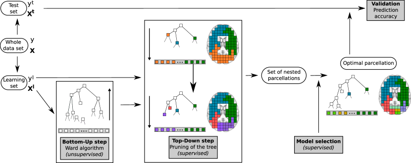
Figure 1: Flowchart of the supervised clustering approach. Bottom-Up step (Ward clustering) - step 2.1.1: the tree $\mathcal{T}$ is constructed from the leaves (the voxels in the gray box) to the unique root (i.e. the full brain volume), following spatial connectivity constraints. Top-Down step (Pruning of the tree) - step 2.1.2: the Ward’s tree is cut recursively into smaller sub-trees, each one corresponding to a parcellation, in order to maximize a prediction accuracy $\zeta$. Model selection - step 2.1.3: given the set of nested parcellations obtained by the pruning step, we select the optimal sub-tree $\widehat{\mathcal{T}}$, i.e. the one that yields the optimal value for $\zeta$.

2.1.1 Bottom-Up step: hierarchical clustering

In the first step, we ignore the target information – i.e. the behavioral variable to be predicted – and use a hierarchical agglomerative clustering. We add connectivity constraints to this algorithm (only adjacent clusters can be merged together) so that only spatially connected clusters, i.e. parcels, are created. This approach creates a hierarchy of parcels represented as a tree $\mathcal{T}$ (or dendrogram) [28]. As the resulting nested parcel sets is isomorphic to the tree $\mathcal{T}$, we identify any tree cut with a given parcellation of the domain. The root of the tree is the unique parcel that gathers all the voxels, the leaves being the parcels with only one voxel. Any cut of the tree into $\delta$ sub-trees corresponds to a unique parcellation $\mathcal{P}_{\delta}$, through which the data can be reduced to $\delta$ parcels-based averages. Among different hierarchical agglomerative clustering, we use the variance-minimizing approach of Ward algorithm [27] in order to ensure that parcel-based averages provide a fair representation of the signal within each parcel. At each step, we merge together the two parcels so that the resulting parcellation minimizes the sum of squared differences within all parcels (inertia criterion).

2.1.2 Top-Down step: pruning of the tree $\mathcal{T}$

We now detail how the tree $\mathcal{T}$ can be pruned to create a reduced set of parcellations. Because the hierarchical subdivision of the brain volume (by successive inclusions) is naturally identified as a tree $\mathcal{T}$, choosing a parcellation adapted to the prediction problem means optimizing a cut of the tree. Each sub-tree created by the cut represents a region whose average signal is used for prediction. As no optimal solution is currently available to solve this problem, we consider two approaches to perform such a cut (see Fig. 2). In order to have $\Delta$ parcels, these two methods start from the root of the tree $\mathcal{T}$ (one unique parcel for the whole brain), and iteratively refine the parcellation:

• The first solution consists in using the inertia criterion from Ward algorithm: the cut consists in a subdivision of the Ward’s tree into its $\Delta$ main branches. As this does not take into account the target information $\mathbb{y}$, we call it unsupervised cut (UC).

• The second solution consists in initializing the cut at the highest level of the hierarchy and then successively finding the new sub-tree cut that maximizes a prediction score $\zeta$ (e.g. explained variance, see Eq.(15) below), while using a prediction function $\mathcal{F}$ (e.g. Support Vector Machine [29]) instantiated with the parcels-based signal averages at the current step. As in a greedy approach, successive cuts iteratively create a finer parcellation of the search volume, yielding the set of parcellations $\mathcal{P}_{1},..,\mathcal{P}_{\Delta}$. More specifically, one parcel is split at each step, where the choice of the split is driven by the prediction problem. After $\delta$ such steps of exploration, the brain is divided into $\delta+1$ parcels. This procedure, called supervised cut (SC), is detailed in algorithm 1.

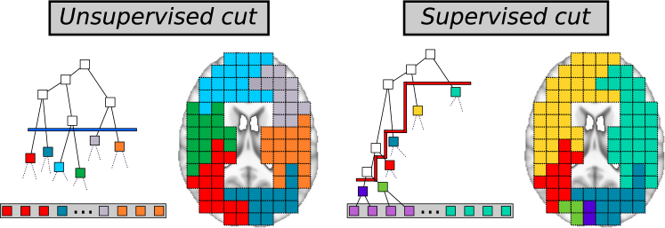
Figure 2: Top-Down step (Pruning of the tree) - step 2.1.2. In the unsupervised cut approach, (left) Ward’s tree is divided into $6$ parcels through a horizontal cut (blue). In the supervised cut approach (right), by choosing the best cut (red) of the tree given a score function $\zeta_{e}$, we focus on some specific regions of the tree that are more informative.

2.1.3 Model Selection step: optimal sub-tree $\widehat{\mathcal{T}}$

In both cases, a set of nested parcellations is produced, and the optimal model among the available cuts still has to be chosen. We select the sub-tree $\widehat{\mathcal{T}}$ that yields the optimal prediction score $\widehat{\zeta}$. The corresponding optimal parcellation is then used to create parcels on both training and test sets. A prediction function is thus trained and tested on these two set of parcels to compute the prediction accuracy of the framework.

2.2 Algorithmic considerations

The pruning of the tree and the model selection step are included in an internal cross-validation procedure within the training set. However, this internal cross-validation scheme rises different issues. First, it is very time consuming to include the two steps within a complete internal cross-validation. A second, and more crucial issue, is that performing an internal cross-validation over the two steps yields many different sub-trees (one by fold). However, it is not easy to combine these different sub-trees in order to obtain an average sub-tree that can be used for prediction on the test set [30]. Moreover, the different optimal sub-trees are not constructed using all the training set, and thus depend on the internal cross-validation scheme. Consequently, we choose an empirical, and potentially biased, heuristic that consists of using sequentially two separate cross-validation schemes $C_{e}$ and $C_{s}$ for the pruning of the tree and the model selection step.

2.3 Computational considerations

Our algorithm can be used to search informative regions in very high-dimensional data, where other algorithms do not scale well. Indeed, the highest number of features considered by our approach is $\Delta$, and we can use any given prediction function $\mathcal{F}$, even if this function is not well-suited for high dimensional data. The computational complexity of the proposed supervised clustering algorithm depends thus on the complexity of the prediction function $\mathcal{F}$, and on the two cross-validation schemes $C_{e}$ and $C_{s}$. At the current iteration $\delta\in[1,\Delta]$, $\delta+1$ possible features are considered in the regression model, and the regression function is fit $n(\delta+1)$ times (in the case of a leave-one-out cross-validation with $n$ samples). Assuming the cost of fitting the prediction function $\mathcal{F}$ is $\mathcal{O}(\delta^{\alpha})$ at step $\delta$, the overall cost complexity of the procedure is $\mathcal{O}(n\Delta^{(2+\alpha)})$. In general $\Delta\ll p$, and the cost remains affordable as long as $\Delta<10^{3}$, which was the case in all our experiments. Higher values for $\Delta$ might also be used, but the complexity of $\mathcal{F}$ has to be lower.

The benefits of parcellation come at a cost regarding CPU time. On a subject of the dataset on the prediction of size (with a non optimized Python implementation though), with $\sim 7.10^{4}$ voxels, the construction of the tree raising CPU time to $207$ seconds and the parcels definition raising CPU time (Intel(R) Xeon(R), 2.83GHz) to $215$ seconds. Nevertheless, all this remains perfectly affordable for standard neuroimaging data analyzes.

Set a number of exploration steps $\Delta$, a score function $\zeta$, a prediction function $\mathcal{F}$, and two cross-validation schemes $C_{e}$ and $C_{s}$.

Let $\mathcal{P}_{\delta}$ be the parcellation defined at the current iteration $\delta$ and $\mathbb{X_{p}}_{\delta}$ the corresponding parcel-based averages.

Construct $\mathcal{T}$ using Ward algorithm.

Start from the root of the tree $\mathcal{T}$, i.e. $\mathcal{P}_{0}=\{P_{0}\}$ has only one parcel $P_{0}$ that contains all the voxels.

Pruning of the tree $\mathcal{T}$

for $\delta\leftarrow 1$ to $\Delta$ do

       foreach $P_{i}\in\mathcal{P}_{\delta-1}$ do

             - Split $P_{i}\rightarrow\{P_{i}{{}^{1}},P_{i}{{}^{2}}\}$ according to $\mathcal{T}$.

             - Set $\mathcal{P}_{\delta,i}=\{\mathcal{P}_{\delta-1}\backslash P_{i}\}\cup\{P_{i}{{}^{1}},P_{i}{{}^{2}}\}$.

             - Compute the corresponding parcel-based signal averages $\mathbb{X_{p}}_{\delta,i}$.

             - Compute the cross-validated score $\zeta_{e,i}(\mathcal{F})$ with the cross-validation scheme $C_{e}$.

      - Perform the split $i^{\star}$ that yields the highest score $\zeta_{e,i^{\star}}(\mathcal{F})$.

       - Keep the corresponding parcellation $\mathcal{P}_{\delta}$ and sub-tree $\mathcal{T}_{\delta}$.

Selection of the optimal sub-tree $\widehat{\mathcal{T}}$

for $\delta\leftarrow 1$ to $\Delta$ do

       - Compute the cross-validated score $\zeta_{s,\delta}(\mathcal{F})$ with the cross-validation scheme $C_{s}$, using the parcellation $\mathcal{P}_{\delta}$.

Return the sub-tree $\widehat{\mathcal{T}}_{\delta^{\star}}$ and corresponding parcellation $\widehat{\mathcal{P}}_{\delta^{\star}}$, that yields the highest score $\zeta_{s,\delta^{\star}}(\mathcal{F})$.

Algorithm 1 Pseudo-code for supervised cut

2.4 Performance evaluation

Our method is evaluated with a cross-validation procedure that splits the available data into training and validation sets. In the following, $(\mathbb{X}^{l},\mathbb{y}^{l})$ are a learning set, $(\mathbb{X}^{t},\mathbb{y}^{t})$ a test set and $\mathbb{\hat{y}}^{t}=f(\mathbb{X}^{t}\mathbb{\hat{w}})$ refers to the predicted target, where $\mathbb{\hat{w}}$ is estimated from the training set. For regression analysis, the performance of the different models is evaluated using $\zeta$, the ratio of explained variance:

$$\zeta(\mathbb{y}^{t},\mathbb{\hat{y}}^{t})=\frac{\mbox{var}(\mathbb{y}^{t})-\mbox{var}\left(\mathbb{y}^{t}-\mathbb{\hat{y}}^{t}\right)}{\mbox{var}(\mathbb{y}^{t})}$$ (15)

This is the amount of variability in the response that can be explained by the model. A perfect prediction yields $\zeta=1$, a constant prediction yields $\zeta=0$). For classification analysis, the performance of the different models is evaluated using a standard classification score denoted $\kappa$ , defined as:

$$\kappa(\mathbb{y}^{t},\mathbb{\hat{y}}^{t})=\frac{\sum_{i=1}^{n^{t}}\delta(y^{t}_{i},\hat{y}_{i}^{t})}{n^{t}}$$ (16)

where $n^{t}$ is the number of samples in the test set, and $\delta$ is Kronecker’s delta.

2.5 Competing methods

In our experiments, the supervised clustering is compared to different state of the art regularization methods. For regression experiments:

• Elastic net regression [31], requires setting two parameters $\lambda_{1}$ (amount of $\ell_{1}$ norm regularization) and $\lambda_{2}$ (amount of $\ell_{2}$ norm regularization). In our analyzes, an internal cross-validation procedure on the training set is used to optimize $\lambda_{1}\in\{0.2\tilde{\lambda},0.1\tilde{\lambda},0.05\tilde{\lambda},0.01\tilde{\lambda}\}$, where $\tilde{\lambda}=\|\mathbb{X}^{T}\mathbb{y}\|_{\infty}$, and $\lambda_{2}\in\{0.1,0.5,1.,10.,100.\}$.

• Support Vector Regression (SVR) with a linear kernel [29], which is the reference method in neuroimaging. The regularization parameter $C$ is optimized by cross-validation in the range of $10^{-3}$ to $10$ in multiplicative steps of $10$.

For classification settings:

• Sparse multinomial logistic regression (SMLR) classification [32], that requires an optimization similar to Elastic Net (two parameters $\lambda_{1}$ and $\lambda_{2}$).

• Support Vector Classification (SVC), which is optimized similarly as SVR.

All these methods are used after an Anova-based feature selection as this maximizes their performance. Indeed, irrelevant features and redundant information can decrease the accuracy of a predictor [33]. This selection is performed on the training set, and the optimal number of voxels is selected in the range $\{50,100,250,500\}$ within a nested cross-validation. We also check that increasing the range of voxels (i.e. adding 2000 in the range of number of selected voxels) does not increase the prediction accuracy on our real datasets. The implementation of Elastic net is based on coordinate descent [34], while SVR and SVC are based on LibSVM [35]. Methods are used from Python via the Scikit-learn open source package [36]. Prediction accuracies of the different methods are compared using a paired t-test.

3 Simulated data

3.1 Simulated one-dimensional data

We illustrate the supervised clustering on a simple simulated data set, where the informative features have a block structure:

$$\mathbb{X}\sim\mathcal{N}(0,1)\;\;\mbox{and}\;\;\mathbb{y}=\mathbb{X}\mathbb{w}+\mathbb{\epsilon}$$ (17)

with $\mathbb{\epsilon}\sim\mathcal{N}(0,1)$ and $\mathbb{w}$ is defined as $w_{i}\sim\mathcal{U}_{0.75}^{1.25}$ for $20\leq i\leq 30$, $w_{i}\sim\mathcal{U}_{-1.25}^{-0.75}$ for $50\leq i\leq 60$, and $w_{i}=0$ elsewhere, where $\mathcal{U}_{a}^{b}$ is the uniform distribution between $a$ and $b$. We have $p=200$ features and $n=150$ images. The supervised cut is used with $\Delta=50$, Bayesian Ridge Regression (BRR) as prediction function $\mathcal{F}$, and procedures $C_{e}$ and $C_{s}$ are set to 4-fold cross-validation.

3.2 Simulated neuroimaging data

The simulated data set $\mathbb{X}$ consists in $n=100$ images (size $12\times 12\times 12$ voxels) with a set of four cubic Regions of Interest (ROIs) (size $2\times 2\times 2$). We call $\mathcal{R}$ the support of the ROIs (i.e. the $32$ resulting voxels of interest). Each of the four ROIs has a fixed weight in $\{-0.5,0.5,-0.5,0.5\}$. We call $w_{i,j,k}$ the weight of the $(i,j,k)$ voxel. To simulate the spatial variability between images (inter-subject variability, movement artifacts in intra-subject variability), we define a new support of the ROIs, called $\tilde{\mathcal{R}}$ such as, for each image, half (randomly chosen) of the weights $\mathbb{w}$ are set to zero. Thus, we have $\tilde{\mathcal{R}}\subset\mathcal{R}$. We simulate the signal in the $(i,j,k)$ voxel of the $l^{th}$ image as:

$$\mathbb{X}_{i,j,k,l}\sim\mathcal{N}(0,1)$$ (18)

The resulting images are smoothed with a Gaussian kernel with a standard deviation of $2$ voxels, to mimic the correlation structure observed in real fMRI data. The target $\mathbb{y}$ for the $l^{th}$ image is simulated as:

$$\mathbb{y}_{l}=\sum_{(i,j,k)\in\tilde{\mathcal{R}}}w_{i,j,k}\mathbb{X}_{i,j,k,l}+\epsilon_{l}$$ (19)

and $\epsilon_{l}\sim\mathcal{N}(0,\gamma)$ is a Gaussian noise with standard deviation $\gamma>0.$ We choose $\gamma$ in order to have a signal-to-noise (SNR) ratio of $5$ dB. The SNR is defined here as $20$ times the log of the ratio between the norm of the signal and the norm of the added noise. We create a training set of $100$ images, and then we validate on $100$ other images simulated according to Eq. 18-19. We compare the supervised clustering approach with the unsupervised clustering and the two reference algorithms, Elastic net and SVR. The two reference methods are optimized by 4-fold cross-validation within the training set in the range described below. We also compare the methods to a searchlight approach [10] (radius of $2$ and $3$ voxels, combined with a SVR approach ($C=1$)), which has emerged as a reference approach for decoding local fine-grained information within the brain.

Both supervised cut and unsupervised cut algorithms are used with $\Delta=50$, Bayesian Ridge Regression (BRR) as prediction function $\mathcal{F}$, and optimized with an internal 4-fold cross-validation.

3.3 Results on one-dimensional simulated data

The results of the supervised clustering algorithm are given in Fig. 4. On the top, we give the tree $\mathcal{T}$, where the parcels found by the supervised clustering are represented by red squares, and the bottom row are the input features. The features of interest are represented by green dots. We note that the algorithm focuses the parcellation on two sub-regions, while leaving other parts of the tree unsegmented. The weights found by the prediction function based on the optimal parcellation (bottom) clearly outlines the two simulated informative regions. The predicted weights are normalized by the number of voxels in each parcel.

3.4 Results on simulated neuroimaging data

We compare different methods on the simulated data, see Fig. 4. The predicted weights of the two parcel-based approaches are normalized by the number of voxels in each parcel. Only the supervised clustering (e) extracts the simulated discriminative regions. The unsupervised clustering (f) does not retrieve the whole support of the weights, as the created parcels are constructed based only on the signal and spatial information, and thus do not consider the target to be predicted. Elastic net (h) only retrieves part of the support of the weights, and yields an overly sparse solution which is not easy to interpret. SVR (g) approach yields weights in the primal space that depend on the smoothness of the images. The searchlight approach (c,d), which is a commonly used brain mapping techniques, shows here its limits: it does not cope with the long range multivariate structure of the weights, and yields very blurred informative maps, because this method naturally degrades data resolution.

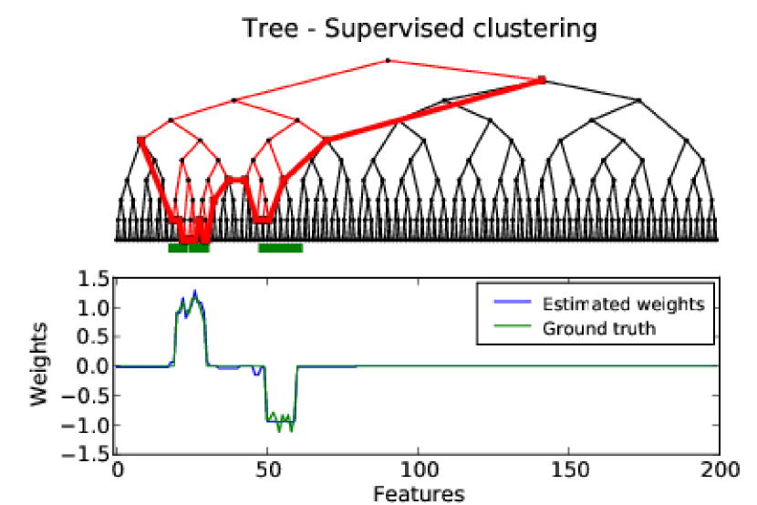
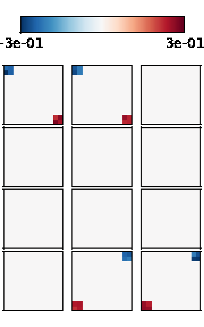
Figure 3: Illustration of the supervised clustering algorithm on a simple simulated data set. The cut of the tree (top, red line) focuses on the regions of interest (top, green dots), which allows the prediction function to correctly weight the informative features (bottom).

(a) True
weights

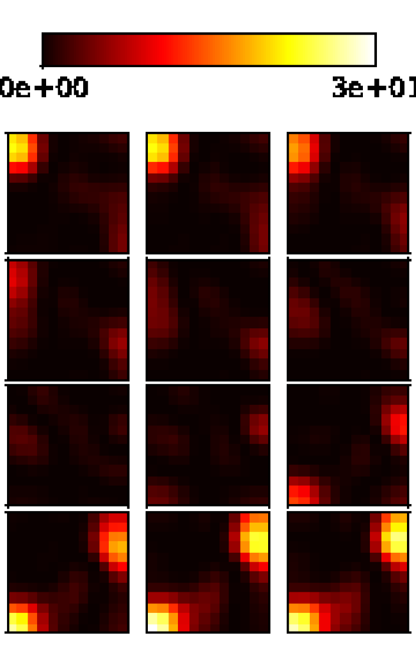
(b) Anova
F-scores

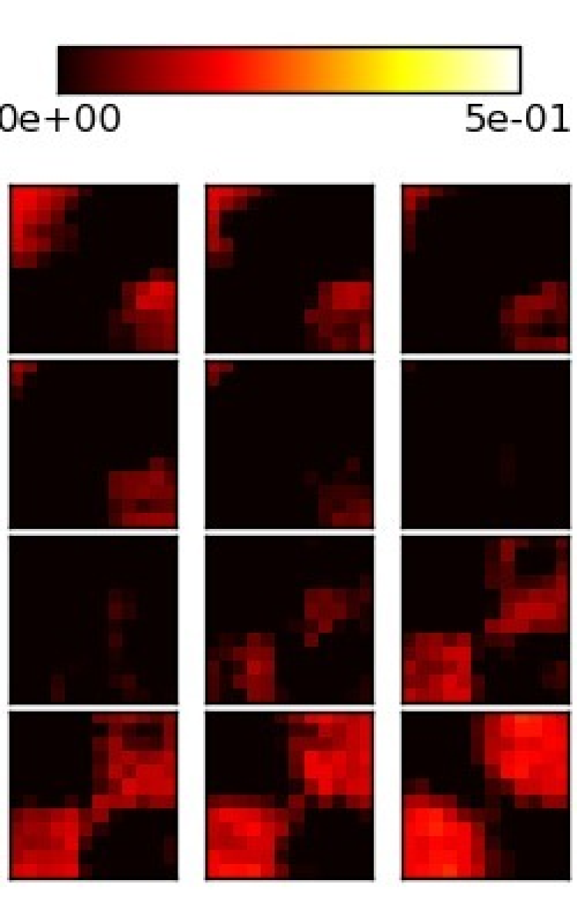
(c) Searchlight
SVR ($r=2$)

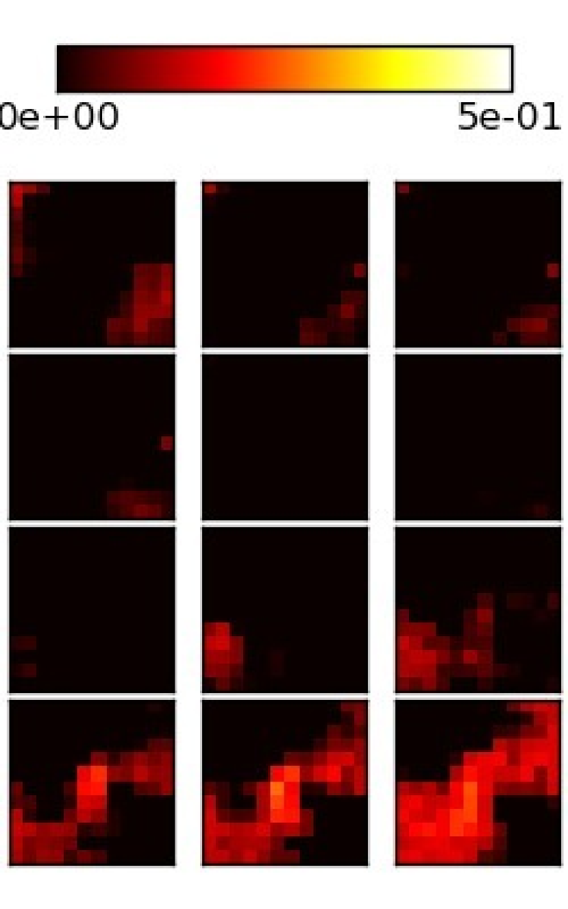
(d) Searchlight
SVR ($r=3$)

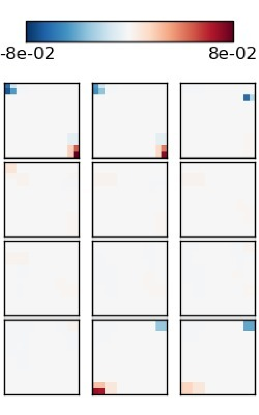
(e) Supervised
clustering

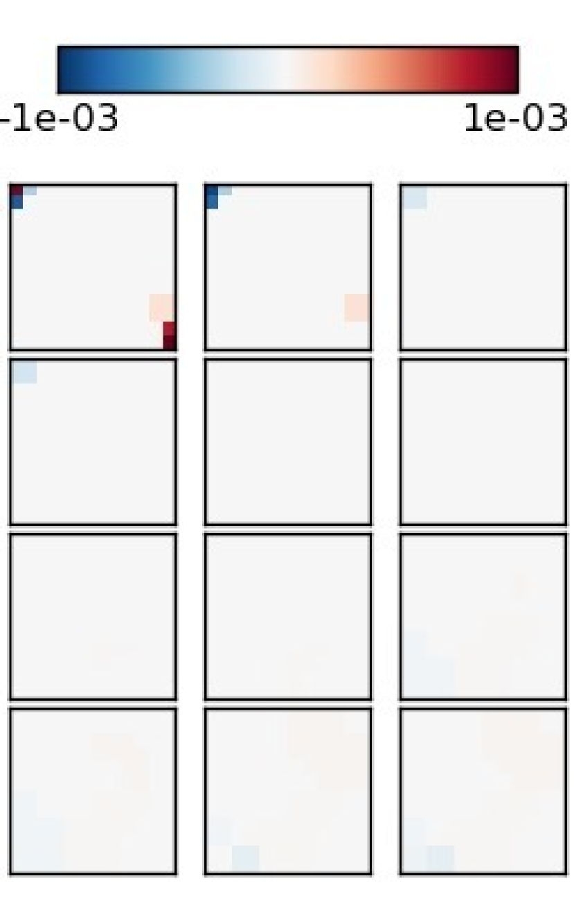
(f) Unsupervised
clustering

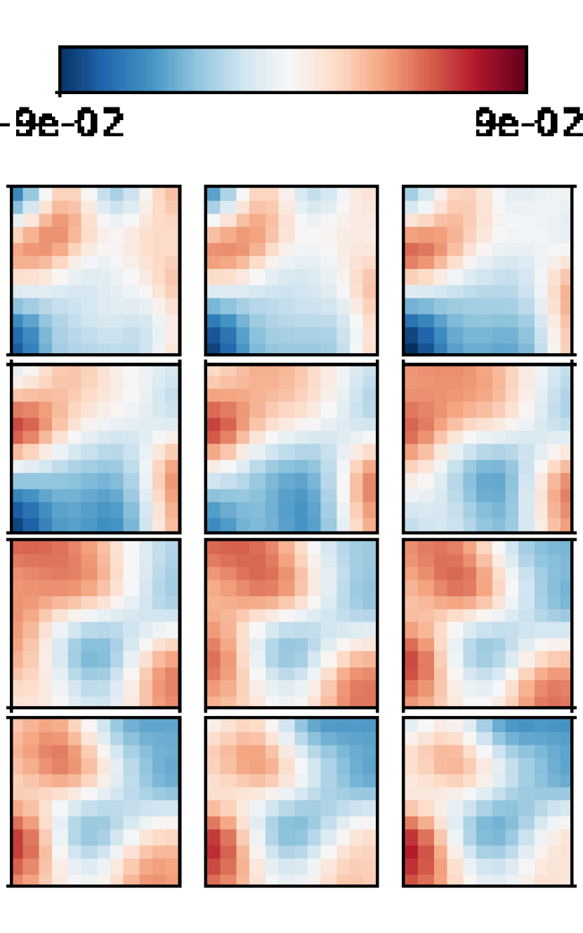
(g) SVR
Cross-validated

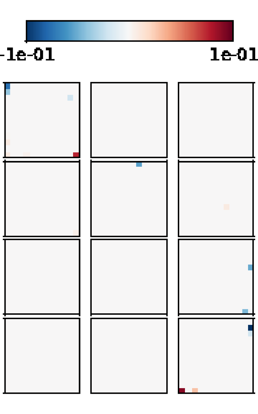
(h) Elastic net
Cross-validated

Figure 4: Comparisons of the weights given by the different procedures (b-h) with the true weights (a). Only the supervised cut algorithm (e) retrieves the regions of interest. For the searchlight approach (c, f), the images show the explained variance obtained using the voxels within a sphere centered on each voxel.

4 Experiments and results on real data

4.1 Details on real data

We apply the different methods to analyze ten subjects from an fMRI dataset related to the study of the visual representation of objects in the brain (see [37] for details). During the experiment, ten healthy volunteers viewed objects of two categories (each one of the two categories is used in half of the subjects) with four different exemplars in each category. Each exemplar was presented at three different sizes (yielding $12$ different experimental conditions per subject). Each stimulus was presented four times in each of the six sessions. We averaged data from the four repetitions, resulting in a total of $n=72$ images by subject (one image of each stimulus by session). Functional images were acquired on a 3-T MR system with eight-channel head coil (Siemens Trio, Erlangen, Germany) as T2*-weighted echo-planar image (EPI) volumes. Twenty transverse slices were obtained with a repetition time of 2s (echo time, 30ms; flip angle, $70^{\circ}$; $2\times 2\times 2$-mm voxels; $0.5$-mm gap). Realignment, normalization to MNI space, and General Linear Model (GLM) fit were performed with the SPM5 software. In the GLM, the time course of each of the $12$ stimuli convolved with a standard hemodynamic response function was modeled separately, while accounting for serial auto-correlation with an AR(1) model and removing low-frequency drift terms with a high-pass filter with a cut-off of 128 s. In the present work we used the resulting session-wise parameter estimate images. All the analysis are performed on the whole brain volume.

Regression experiments: The four different exemplars in each of the two categories were pooled, leading to images labeled according to the 3 possible sizes of the object. By doing so, we are interested in finding discriminative information to predict the size of the presented object. This reduces to a regression problem, in which our goal is to predict a simple scalar factor (size or scale of the presented object).

We perform an inter-subject regression analysis on the sizes. This analysis relies on subject-specific fixed-effects activations, i.e. for each condition, the six activation maps corresponding to the six sessions are averaged together. This yields a total of twelve images per subject, one for each experimental condition. The dimensions of the real data set are $p\sim 7\times 10^{4}$ and $n=120$ (divided into three different sizes). We evaluate the performance of the method by cross-validation (leave-one-subject-out). The parameters of the reference methods are optimized with a nested leave-one-subject-out cross-validation within the training set, in the ranges given before. The supervised clustering and unsupervised clustering are used with Bayesian Ridge Regression (BRR) (as described in section 3.3 in [38]) as prediction function $\mathcal{F}$. Internally, a leave-one-subject-out cross-validation is used and we set the maximal number of parcels to $\Delta=75$. The optimal number of parcels is thus selected between $1$ and $75$ by a nested cross-validation loop.

A major asset of BRR is that it adapts the regularization to the data at hand, and thus can cope with the different dimensions of the problem: in the first steps of the supervised clustering algorithm, we have more samples than features, and for the last steps, we have more features than samples. The two hyperparameters that governed the gamma distribution of the regularization term of BRR are both set to $10^{-6}$ (the prior is weakly informative). We do not optimize these hyperparameters, due to computational considerations, but we check that with more informative priors we obtain similar results in the regression experiment ($0.81$ and $0.79$ with respectively $\lambda_{1}=\lambda_{2}=0.01$ and $\lambda_{1}=\lambda_{2}=1.$).

Classification experiments: We evaluate the performance on a second type of discrimination which is object classification. In that case, we averaged the images for the three sizes and we are interested in discriminating between individual object shapes. For each of the two categories, this can be handled as a classification problem, where we aim at predicting the shape of an object corresponding to a new fMRI scan. We perform two analyses corresponding to the two categories used, each one including five subjects.

In this experiment, the supervised clustering and unsupervised clustering are used with SVC ($C=0.01$) as prediction function $\mathcal{F}$. Such value of $C$ yields a good regularization of the weights in the proposed approach, and the results are not too sensitive to this parameter ($67.5\%$ for $C=10$)

4.2 Results for the prediction of size

The results of the inter-subjects analysis are given in Tab.2. Both parcel-based methods perform better than voxel-based reference methods. Parcels can be seen as an accurate method for compressing information without loss of prediction performance. Fig. 5 gives the weights found for the supervised cut, the two reference methods and the searchlight ($SVR$ with $C=1$ and a radius of $2$ voxels), using the whole data set. As one can see, the proposed algorithm yields clustered loadings map, compared to the maps yielded by the voxel-based methods, which are very sparse and difficult to represent. Compared to the searchlight, the supervised clustering creates more clusters that are also easier to interpret as they are well separated. Moreover, the proposed approach yields a prediction accuracy for the whole brain analysis, a contrario to the searchlight that only gives a local measure of information.

The majority of informative parcel are located in the posterior part of the occipital cortex, most likely corresponding to primary visual cortex, with few additional slightly more anterior parcels in posterior lateral occipital cortex. This is consistent with the previous findings [37] where a gradient of sensitivity to size was observed across object selective lateral occipital ROIs, while the most accurate discrimination of sizes is obtained in primary visual cortex.

Methods	mean $\zeta$	std $\zeta$	max $\zeta$	min $\zeta$	p-val to UC
SVR	$0.77$	$0.11$	$0.97$	$0.58$	$0.0817$
Elastic net	$0.78$	$0.1$	$0.97$	$0.65$	$0.0992$
UC - BRR	$0.83$	$0.08$	$0.97$	$0.73$	-
SC - BRR	$0.82$	$0.08$	$0.93$	$0.7$	$0.8184$

Table 1: Explained variance $\zeta$ for the different methods in the Size prediction analysis. The p-values are computed using a paired t-test. The unsupervised cut (UC) algorithm yields the best prediction accuracy (leave-one-subject-out cross-validation). The supervised cut (SC) yields similar results as UC (the difference is not significant). The two voxel-based approaches yield lower prediction accuracy than parcel-based approaches.

Methods	mean $\kappa$	std $\kappa$	max $\kappa$	min $\kappa$	p-val to SC
SVC	$48.33$	$15.72$	$75.0$	$25.0$	$0.0063$ **
SMLR	$42.5$	$9.46$	$58.33$	$33.33$	$0.0008$ **
UC - SVC	$65.0$	$8.98$	$75.0$	$50.0$	$0.1405$
SC - SVC	$70.0$	$10.67$	$83.33$	$50.0$	-

Methods	mean (std) $\kappa$	mean (std) $\kappa$	Mean nb. feat.
	cat. 1	cat.2	(voxels/parcels)
SVC	$56.6(17.8)$	$40.0(6.2)$	$415$
SMLR	$43.3(9.7)$	$41.6(9.1)$	$150$
UC - SVC	$63.3(8.5)$	$68.3(9.7)$	$21$
SC - SVC	$65(12.2)$	$75(5.2)$	$17$

Table 2: Top – Classification performance $\kappa$ for the different methods in the Object prediction analysis. The p-values are computed using a paired t-test. The supervised cut (SC) algorithm yields the best prediction accuracy (leave-one-subject-out cross-validation). Both parcels-based approaches are significantly more accurate and more stable than voxel-based approaches. Bottom – Details of the results for the two categories and mean number of features (voxels or parcels) for the different methods. We can notice that parcels yield a good compression of information has with more than ten times less features, parcel-based approaches yield higher prediction accuracy.

4.3 Results for the prediction of shape

The results of the inter-subjects analysis are given in Tab.2. The supervised cut method outperforms the other approaches. In particular, the classification score is $21\%$ higher than with voxel-based SVC and $27\%$ higher than with voxel-based SMLR. Both parcel-based approaches are significantly more accurate and more stable than the voxel-based approaches. The number of features used show the good compression of information performed by the parcels. With ten times less features than voxel-based approaches, the prediction accuracies of parcel-based approaches are higher. The lower performances of SVC and SMLR can be explained by the fact that voxel-based approaches can not deal with inter-subject variability, especially in such cases where information can be encoded in pattern of voxels that can vary spatially across subjects.

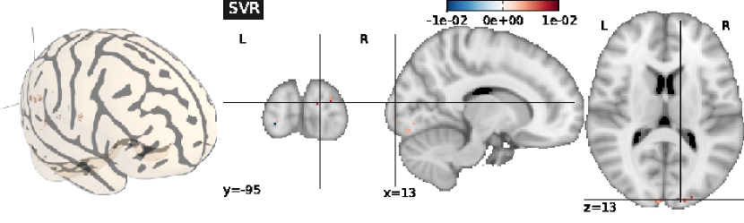
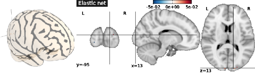
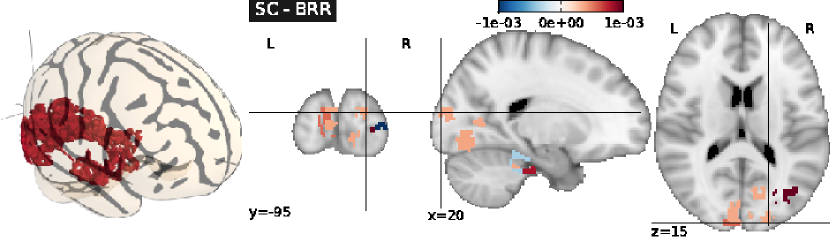
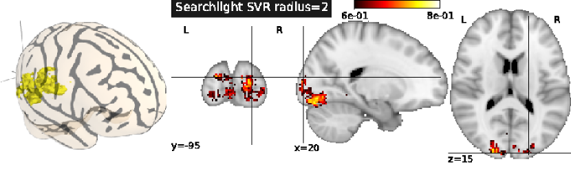
Figure 5: Results for prediction of size. Maps of weights found by supervised cut, the two reference voxel-based methods and the searchlight. The proposed algorithm creates very interpretable clusters, compared to the reference methods, which is related to the fact that they do not consider the spatial structure of the image. Moreover, the supervised clustering yields similar maps as searchlight, but also retrieves some additional clusters.

5 Discussion

In this paper, we have presented a new method for enhancing the prediction of experimental variables from fMRI brain images. The proposed approach constructs parcels (groups of connected voxels) by feature agglomeration within the whole brain, and allows to take into account both the spatial structure and the multivariate information within the whole brain.

Given that an fMRI brain image has typically $10^{4}$ to $10^{5}$ voxels, it is perfectly reasonable to use intermediate structures such as parcels for reducing the dimensionality of the data. We also confirmed by different experiments that parcels are a good way to tackle the spatial variability problem in inter-subjects studies. Thus feature agglomeration is an accurate approach for the challenging inter-subject generalization of brain-reading [39, 4]. This can be explained by the fact that considering parcels allows to localize functional activity across subjects and thus find a common support of neural codes of interest (see Fig. 6). On the contrary, voxel-based methods suffer from the inter-subject spatial variability and their performances are relatively lower.

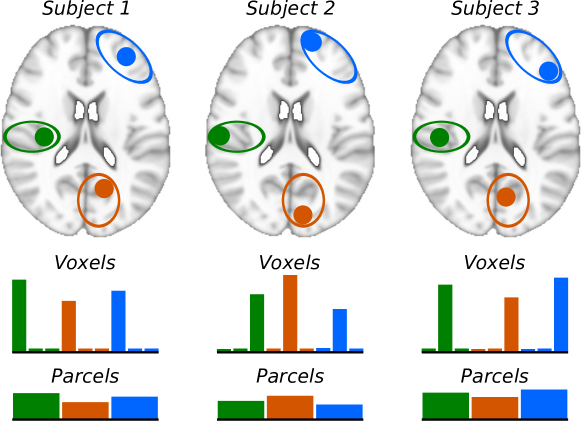
Figure 6: Illustration of feature agglomeration to cope with inter-subject variability. The regions implied in the cognitive task are represented by disks of different colors. The populations of active neurons are not exactly at the same position across subjects (top), and the across subjects mean signal in informative voxels (bottom) carries very weak information. Thus, it is clear that, in this case, voxel-based decoding approaches will perform poorly. However, the mean of informative voxels within each region across subjects (bottom) carries more information and should yield an accurate inter-subject prediction.

Our approach entails the technical difficulty of optimizing the parcellation with respect to the spatial organization of the information within the image. To break the combinatorial complexity of the problem, we have defined a recursive parcellation of the volume using Ward algorithm, which is furthermore constrained to yield spatially connected clusters. Note that it is important to define the parcellation on the training database to avoid data overfit. The sets of possible volume parcellations is then reduced to a tree, and the problem reduces to finding the optimal cut of the tree. We propose a supervised cut approach that attempts to optimize the cut with respect to the prediction task. Although finding an optimal solution is infeasible, we adopt a greedy strategy that recursively finds the splits that most improve the prediction score. However, there is still no guarantee that the optimal cut might be reached with this strategy. Model selection is then performed a posteriori by considering the best generalizing parcellation among the available models. Additionally, our method is tractable on real data and runs in a very reasonable of time (a few minutes without specific optimization).

In terms of prediction accuracy, the proposed methods yield better results for the inter-subjects study on the different experiments, compared to state of the art approaches (SVR, Elastic net, SVC and SMLR). The supervised cut yields similar or higher prediction accuracy than the unsupervised cut. In the size prediction analysis, the information is probably coarser than in the object prediction analysis, and thus the simple heuristic of unsupervised cut yields a good prediction accuracy. Indeed, the unsupervised clustering still optimizes a cost function by selecting the number of parcels that maximizes the prediction accuracy. Thus, in simple prediction task such as the regression problem detailed in this article, this approach allows to extract almost all the relevant information. However, in the prediction of more fine-grained information, such as in the classification task, the UC procedure does not provide a sufficient exploration of the different parcellations, and does not extract all the relevant information. Contrariwise, the SC approach explores relevant parcellations using supervised information, and thus performs better than UC.

In terms of interpretability, we have shown on simulations and real data that this approach has the particular capability to highlight regions of interest, while leaving uninformative regions unsegmented, and it can be viewed as a multi-scale segmentation scheme [26]. The proposed scheme is further useful to locate contiguous predictive regions and to create interpretable maps, and thus can be viewed as an intermediate approach between brain mapping and inverse inference. Moreover, compared to a state of the art approach for fine-grained decoding, namely the searchlight, the proposed method yields similar maps, but additionally, takes into account non-local information and yields only one prediction score corresponding to whole brain analysis. From a neuroscientific point of view, the proposed approach retrieves well-known results, i.e. that differences between sizes (or between stimuli with different spatial envelope in general) are most accurately represented in the signals of early visual regions that have small and retinotopically laid-out receptive fields.

More generally, this approach is not restricted to a given prediction function and can be used with many different classification/regression methods. Indeed, by restricting the search of the best subset of voxels to a tree pruning problem, our algorithm allows us to guide the construction of the prediction function in a low-dimensional representation of a high-dimensional dataset. Moreover, this method is not restricted to brain images, and might be used in any dataset where multi-scale structure is considered as important (e.g. medical or satellite images).

In conclusion, this paper proposes a method for extracting information from brain images, that builds relevant features by feature agglomeration rather than simple selection. A particularly important property of this approach is its ability to focus on relatively small but informative regions while leaving vast but uninformative areas unsegmented. Experimental results demonstrate that this algorithm performs well for inter-subjects analysis where the accuracy of the prediction is tested on new subjects. Indeed, the spatial averaging of the signal induced by the parcellation appears as a powerful way to deal with inter-subject variability.

References

- [1] D. D. Cox, R. L. Savoy, Functional magnetic resonance imaging (fMRI) ”brain reading”: detecting and classifying distributed patterns of fMRI activity in human visual cortex, NeuroImage 19 (2) (2003) 261–270.
- [2] Y. Kamitani, F. Tong, Decoding the visual and subjective contents of the human brain, Nature Neuroscience 8 (5) (2005) 679–685.
- [3] P. Dayan, L. F. Abbott, Theoretical Neuroscience: Computational and Mathematical Modeling of Neural Systems, The MIT Press, 2001.
- [4] J.-D. Haynes, G. Rees, Decoding mental states from brain activity in humans, Nature Reviews Neuroscience 7 (2006) 523–534.
- [5] M. K. Carroll, G. A. Cecchi, I. Rish, R. Garg, A. R. Rao, Prediction and interpretation of distributed neural activity with sparse models, NeuroImage 44 (1) (2009) 112 – 122.
- [6] K. Friston, A. Holmes, K. Worsley, J. Poline, C. Frith, R. Frackowiak, Statistical parametric maps in functional imaging: A general linear approach, Human Brain Mapping 2 (1995) 189–210.
- [7] D. Cordes, V. M. Haughtou, J. D. Carew, K. Arfanakis, K. Maravilla, Hierarchical clustering to measure connectivity in fmri resting-state data, Magnetic resonance imaging 20 (4) (2002) 305–317.
- [8] M. Palatucci, T. Mitchell, Classification in very high dimensional problems with handfuls of examples, in: Principles and Practice of Knowledge Discovery in Databases (ECML/PKDD), Springer-Verlag, 2007.
- [9] V. Michel, A. Gramfort, G. Varoquaux, B. Thirion, Total Variation regularization enhances regression-based brain activity prediction, in: 1st ICPR Workshop on Brain Decoding 1st ICPR Workshop on Brain Decoding - Pattern recognition challenges in neuroimaging - 20th International Conference on Pattern Recognition, 2010, p. 1.
- [10] N. Kriegeskorte, R. Goebel, P. Bandettini, Information-based functional brain mapping, Proceedings of the National Academy of Sciences of the United States of America 103 (2006) 3863 – 3868.
- [11] G. Flandin, F. Kherif, X. Pennec, G. Malandain, N. Ayache, J.-B. Poline, Improved detection sensitivity in functional MRI data using a brain parcelling technique, in: Medical Image Computing and Computer-Assisted Intervention (MICCAI’02), Vol. 2488 of LNCS, 2002, pp. 467–474.
- [12] T. M. Mitchell, R. Hutchinson, R. S. Niculescu, F. Pereira, X. Wang, M. Just, S. Newman, Learning to decode cognitive states from brain images, Machine Learning V57 (1) (2004) 145–175.
- [13] Y. Fan, D. Shen, C. Davatzikos, Detecting cognitive states from fmri images by machine learning and multivariate classification, in: CVPRW ’06: Proceedings of the 2006 Conference on Computer Vision and Pattern Recognition Workshop, 2006, p. 89.
- [14] B. Thirion, G. Flandin, P. Pinel, A. Roche, P. Ciuciu, J.-B. Poline, Dealing with the shortcomings of spatial normalization: Multi-subject parcellation of fMRI datasets, Hum. Brain Mapp. 27 (8) (2006) 678–693.
- [15] K. Ugurbil, L. Toth, D.-S. Kim, How accurate is magnetic resonance imaging of brain function?, Trends in Neurosciences 26 (2) (2003) 108 – 114.
- [16] D. Kontos, V. Megalooikonomou, D. Pokrajac, A. Lazarevic, Z. Obradovic, O. B. Boyko, J. Ford, F. Makedon, A. J. Saykin, Extraction of discriminative functional MRI activation patterns and an application to alzheimer’s disease, in: Med Image Comput Comput Assist Interv. MICCAI 2004, 2004, pp. 727–735.
- [17] N. Tzourio-Mazoyer, B. Landeau, D. Papathanassiou, F. Crivello, O. Etard, N. Delcroix, B. Mazoyer, M. Joliot, Automated anatomical labeling of activations in spm using a macroscopic anatomical parcellation of the MNI MRI single-subject brain, NeuroImage 15 (1) (2002) 273–289.
- [18] M. Keller, M. Lavielle, M. Perrot, A. Roche, Anatomically Informed Bayesian Model Selection for fMRI Group Data Analysis, in: 12th MICCAI, 2009.
- [19] B. Thyreau, B. Thirion, G. Flandin, J.-B. Poline, Anatomo-functional description of the brain: a probabilistic approach, in: Proc. 31th Proc. IEEE ICASSP, Vol. V, 2006, pp. 1109–1112.
- [20] S. Ghebreab, A. Smeulders, P. Adriaans, Predicting brain states from fMRI data: Incremental functional principal component regression, in: Advances in Neural Information Processing Systems, MIT Press, 2008, pp. 537–544.
- [21] L. He, I. R. Greenshields, An mrf spatial fuzzy clustering method for fmri spms, Biomedical Signal Processing and Control 3 (4) (2008) 327 – 333.
- [22] P. Filzmoser, R. Baumgartner, E. Moser, A hierarchical clustering method for analyzing functional mr images, Magnetic Resonance Imaging 17 (6) (1999) 817 – 826.
- [23] A. Tucholka, B. Thirion, M. Perrot, P. Pinel, J.-F. Mangin, J.-B. Poline, Probabilistic anatomo-functional parcellation of the cortex: how many regions?, in: 11thProc. MICCAI, LNCS Springer Verlag, 2008.
- [24] J.-D. Haynes, G. Rees, Predicting the orientation of invisible stimuli from activity in human primary visual cortex, Nature Neuroscience 8 (5) (2005) 686–691.
- [25] P. Golland, Y. Golland, R. Malach, Detection of spatial activation patterns as unsupervised segmentation of fMRI data, Med Image Comput Comput Assist Interv. MICCAI 2007, 2007, pp. 110–118.
- [26] V. Michel, E. Eger, C. Keribin, J.-B. Poline, B. Thirion, A supervised clustering approach for extracting predictive information from brain activation images, MMBIA’10.
- [27] J. H. Ward, Hierarchical grouping to optimize an objective function, Journal of the American Statistical Association 58 (301) (1963) 236–244.
- [28] S. C. Johnson, Hierarchical clustering schemes, Psychometrika 2 (1967) 241–254.
- [29] C. Cortes, V. Vapnik, Support-vector networks, Machine Learning 20 (3) (995) 273–297.
- [30] J. J. Oliver, D. J. Hand, On pruning and averaging decision trees, in: ICML, 1995, pp. 430–437.
- [31] H. Zou, T. Hastie, Regularization and variable selection via the elastic net, J. Roy. Stat. Soc. B 67 (2005) 301.
- [32] B. Krishnapuram, L. Carin, M. A. Figueiredo, A. J. Hartemink, Sparse multinomial logistic regression: Fast algorithms and generalization bounds, IEEE Transactions on Pattern Analysis and Machine Intelligence 27 (2005) 957–968.
- [33] G. Hughes, On the mean accuracy of statistical pattern recognizers, Information Theory, IEEE Transactions on 14 (1) (1968) 55–63.
- [34] J. Friedman, T. Hastie, R. Tibshirani, Regularization paths for generalized linear models via coordinate descent, Journal of Statistical Software 33 (1).
- [35] C.-C. Chang, C.-J. Lin, LIBSVM: a library for support vector machines, software available at http://www.csie.ntu.edu.tw/~cjlin/libsvm (2001).
- [36] scikit-learn, http://scikit-learn.sourceforge.net/, version 0.2 (downloaded in Apr. 2010).
- [37] E. Eger, C. Kell, A. Kleinschmidt, Graded size sensitivity of object exemplar evoked activity patterns in human loc subregions, J. Neurophysiol. 100(4):2038-47.
- [38] C. M. Bishop, Pattern Recognition and Machine Learning (Information Science and Statistics), 1st Edition, Springer, 2007.
- [39] K. A. Norman, S. M. Polyn, G. J. Detre, J. V. Haxby, Beyond mind-reading: multi-voxel pattern analysis of fmri data., Trends Cogn Sci 10 (9) (2006) 424–430.