Non-Hermitian extensions of Wishart random matrix ensembles

Abstract

We briefly review the solution of three ensembles of non-Hermitian random matrices generalizing the Wishart-Laguerre (also called chiral) ensembles. These generalizations are realized as Gaussian two-matrix models, where the complex eigenvalues of the product of the two independent rectangular matrices are sought, with the matrix elements of both matrices being either real, complex or quaternion real. We also present the more general case depending on a non-Hermiticity parameter, that allows us to interpolate between the corresponding three Hermitian Wishart ensembles with real eigenvalues and the maximally non-Hermitian case. All three symmetry classes are explicitly solved for finite matrix size $N\times M$ for all complex eigenvalue correlations functions (and real or mixed correlations for real matrix elements). These are given in terms of the corresponding kernels built from orthogonal or skew-orthogonal Laguerre polynomials in the complex plane. We then present the corresponding three Bessel kernels in the complex plane in the microscopic large-$N$ scaling limit at the origin, both at weak and strong non-Hermiticity with $M-N\geq 0$ fixed.

1 Introduction and motivation

The Wishart ensemble was the first ensemble of random matrices, introduced in the study of randomized rectangular times series matrices $C$ in order to study the spectral properties of its symmetric and positive covariance matrix $C^{T}C$. Later the Wigner-Dyson ensembles were formulated as models for randomized Hamiltonians $H$ of heavy nuclei to explain some of the spectral properties of the matrix $H$ which is Hermitian (or real symmetric or quaternion self dual). Its non-Hermitian generalizations were introduced and studied immediately after by Ginibre [21], but not so for the Wishart ensembles which had to wait a few decades.

In order to construct such a generalization it is useful to compare to the Ginibre ensembles and to think of them as a two-matrix problem. By dropping the Hermiticity constraint an independent anti-Hermitian matrix $A$ is added to the Hermitian matrix $H$, and the now complex eigenvalues of the sum $H+A$ of the two are studied. How can one repeat this for Wishart matrices, where the matrix $C$ is already without symmetry? Again one can introduce a second independent random matrix $D$, and study this time the complex spectrum of the product $DC$, where $D$ is no longer the transpose (or Hermitian conjugate) of the first matrix, $C^{\dagger}\neq D$, but has the same rectangular dimension.

Interestingly the solution of this two-matrix problem did not grow out of statistical applications, where the problem has appeared in terms of so-called time lagged, asymmetric covariance matrices e.g. in [28, 29, 11]. Non-Hermitian Wishart ensembles also appeared naturally as the described two-matrix problem in the study of the Dirac operator spectrum of Quantum Chromodynamics (QCD) with chemical potential $\mu$. Here the ensemble with complex ($\beta=2$) [32], quaternion real ($\beta=4$) [2], and real ($\beta=1$) [4, 6] matrix elements were first introduced and solved for finite and infinite matrix dimensions by Osborn, the author and his coworkers, respectively. In particular this includes the generalization of the Bessel kernels in the microscopic origin scaling limit into the complex plane for all three ensembles. We refer to [38] for the most recent review on the topic of random matrix applications to QCD. Because the solution of these three ensembles can be expressed in terms of Laguerre polynomials in the complex plane, and because these ensembles display chiral symmetry (see e.g. [38]) they are also called non-Hermitian (or complex) Laguerre or chiral ensembles. The link to statistical applications of non-Hermitian Wishart ensembles was reemphasized more recently in [26]. Here and independently in [12] the spectral density generalizing the Marchenko-Pastur distribution into the complex plane was computed. In [12] the product of having also more than two rectangular matrices was considered.

The two-matrix models constructed and solved for applications to QCD are much more general, for two reasons. First, they depend on a non-Hermiticity parameter (the chemical potential $\mu$) that allows to smoothly deform the Hermitian Wishart (-Laguerre or chiral) ensembles into the maximally non-Hermitian Wishart ensembles of two independent matrices described above. In the Ginibre ensembles these deformations also exist and are called elliptic, or Ginibre-Girko ensembles. The parameter $\mu$ allows to study deformations of the kernels known to be universal from the Hermitian setting. Second, more source terms were added to these parameter dependent two-matrix models, by inserting an arbitrary but fixed number of characteristic polynomials (as additional determinants of the Dirac operator) into the measure. All complex eigenvalue correlation functions were computed in this more general setting in [32, 1] for $\beta=2$, in [2, 3] for $\beta=4$ and in [8, 9] for $\beta=1$. We also mention that the $\beta=1$ symmetry class at maximal non-Hermiticity appears in the superconducting phase of QCD with two colors [24]. In this short presentation we will focus on the first aspect, the dependence on the non-Hermiticity parameter and recall the full solution in terms of (skew) orthogonal polynomials in the complex plane. The additional characteristic polynomials can then be easily implemented by modifying the corresponding kernels (see e.g. in [1, 8]).

Finally we would like to mention some related developments in non-Hermitian random matrices. First of all non-Hermitian generalizations of Wishart ensembles were first considered as one-matrix models [37, 23] where the non-Hermiticity is provided by a constant matrix shift. These models are much more difficult to be solved in general, and only the microscopic density for $\beta=2$ was determined in [36].

Instead of considering the complex eigenvalues of the product of two matrices, in [16] those of the ratio of two matrices were studied, which relate to a Cauchy distribution. When generalizing from one to two Wishart matrices, one can also consider the positive Hermitian (real symmetric) combination $(DC)^{\dagger}DC$, as was done in for instance in [33], including more matrices. Again this generalizes the Marchenko-Pastur density, this times for real eigenvalues, finding generating functions relevant in combinatorics. More generally speaking, spectral properties of the product of quadratic random matrices - Hermitian or non-Hermitian - have been studied by several authors in the literature, and we refer to [14] as well as to the contribution [13] to these proceedings and references therein. The three Ginibre ensembles, and the three non-Hermitian Wishart ensembles reviewed here are not the only possible non-Hermitian random matrices one can consider. For an ordering principle we refer to [10, 30] which include these 6 classes out of 33 non-Hermitian ones. For recent reviews on non-Hermitian random matrices we refer to [27, 39].

This review is organized as follows. In Sect. 2 we recall the definition of generalized non-Hermitian Wishart ensembles, discuss their relation to standard Wishart ensembles and give their complex eigenvalues representations. Sect. 3 gives a list of the three sets of (skew) orthogonal Laguerre polynomials in the complex plane and their kernels that allows to compute all complex (and real) eigenvalue correlation functions. The large-$N$ limit is sketched in Sect. 4, starting with the elliptic law for the Dirac eigenvalues and then listing the three Bessel kernels in the microscopic origin limit at weak and strong non-Hermiticity. A short discussion on universality follows in Sect. 5.

2 Complex eigenvalue representation of the partition function

We begin by recalling the definition of the standard Wishart ensembles we wish to generalize. Its partition function is given by

$$Z_{N,\,\nu}^{(\beta)}\sim\int dC\exp\left[-\frac{N}{2}{\mbox{Tr}}(C^{\dagger}C)\right]\ ,$$ (1)

where $C$ is a rectangular matrix of size $N\times(N+\nu)$ with real ($\beta=1$), complex ($\beta=2$) or quaternion real ($\beta=4$) matrix element without further symmetry. When going to a real eigenvalue basis for these ensembles there are two choices. Either we can consider the $N$ positive eigenvalues $\lambda_{i}$ of the positive Hermitian matrix $C^{\dagger}C$, which we will call Wishart eigenvalues (or Wishart picture). Or we can consider the $2N+\nu$ eigenvalues $x_{i}$ of the Dirac matrix $\hbox to0.0pt{ /\hss}D=\left(\begin{array}[]{cc}\mbox{\bf 0}_{N}&C\\ C^{\dagger}&\mbox{\bf 0}_{N+\nu}\end{array}\right)$ which we call Dirac eigenvalues (or Dirac picture). When comparing the two characteristic equations,

$$\det[\lambda-C^{\dagger}C]=\prod_{i=1}^{N}(\lambda-\lambda_{i})\ ,\ \ \mbox{vs.}\ \ \det[\lambda-\hbox to0.0pt{ /\hss}D]=\lambda^{\nu}\prod_{i=1}^{N}(\lambda^{2}-x_{i}^{2})\ ,$$ (2)

it is clear that we have $\nu$ zero- and $2N$ non-zero Dirac eigenvalues that come in $\pm$ pairs. The simple substitution $\lambda_{i}=x_{i}^{2}$ will lead us from one picture to the other for the non-zero eigenvalues. When computing the standard Jacobian for the diagonalization we obtain the partition function in terms of eigenvalues as follows

$$Z_{N,\,\nu}^{(\beta)} \sim \int_{0}^{\infty}\prod_{i=1}^{N}d\lambda_{i}\lambda_{i}^{\frac{\beta}{2}(\nu+1)-1}e^{-N\lambda_{i}}\ |\Delta_{N}(\{\lambda_{j}\})|^{\beta}$$ (3)

$$\sim \int_{-\infty}^{\infty}\prod_{i=1}^{N}dx_{i}|x_{i}|^{{\beta}(\nu+1)-1}e^{-Nx_{i}^{2}}\ |\Delta_{N}(\{x_{j}^{2}\})|^{\beta}.$$

It is given in both the Wishart and Dirac picture, and we have defined the Vandermonde determinant as

$$\Delta_{N}(\{\lambda_{j}\})\equiv\prod_{N\geq k>l\geq 1}(\lambda_{k}-\lambda_{l})=\det_{1\leq k,l\leq N}\Big{[}\lambda_{k}^{l-1}\Big{]}\ .$$ (4)

Let us now turn to the non-Hermitian generalization. As sketched in the introduction we consider a Gaussian two-matrix model and compute the spectral properties of the non-Hermitian matrix $DC$:

$${\cal Z}_{N,\,\nu}^{(\beta)}\sim\int dCdD\exp\left[-\frac{N}{2}{\mbox{Tr}}(C^{\dagger}C+D^{\dagger}D)\right]\ .$$ (5)

Both $C$ and $D^{\dagger}$ are rectangular matrices of size $N\times(N+\nu)$ with real ($\beta=1$), complex ($\beta=2$) or quaternion real ($\beta=4$) matrix elements without further symmetry. Instead of the $N$ complex eigenvalues $v_{i}$ of the product matrix $DC$ we may again consider the spectrum of the non-Hermitian Dirac matrix $\hbox to0.0pt{ /\hss}D=\left(\begin{array}[]{cc}\mbox{\bf 0}_{N}&C\\ D&\mbox{\bf 0}_{N+\nu}\end{array}\right)$ instead. Here the ensemble ($\beta=1$) has a special feature. The characteristic equation of the real asymmetric matrix $DC$ remains real. Therefore the solutions of $\det[\lambda-DC]=\prod_{i=1}^{N}(\lambda-v_{i})$ are either real, or occur in complex conjugate pairs. For the non-zero complex Dirac eigenvalues $z_{i}$ we thus get 3 different possibilities listed in Table 1.

	Wishart picture	Dirac picture
a)	$v_{j}>0$ real	$\pm z_{j}\in\mathbb{R}$, $z_{j}^{2}=v_{j}$
b)	$v_{j}<0$ real	$\pm z_{j}\in i\mathbb{R}$, $z_{j}^{2}=v_{j}$
c)	$v_{j},\ v_{j}^{*}$ complex conjugate pair	$\pm z_{j},\pm z_{j}^{*}\in\mathbb{C}$, 2 pairs $z_{j}^{2\,(*)}=v_{j}^{(*)}$

Table 1: Non-zero complex eigenvalues for real matrix elements $\beta=1$.

In the following we will solve a more general non-Hermitian extension of the Wishart ensembles than eq. (5). We add a non-Hermiticity parameter $\mu\in[0,1]$ that allows to interpolate between the Wishart ensemble eq. (1) for $\mu=0$ and its generalization eq. (5) for $\mu=1$ which we call maximally non-Hermitian. The partition function is defined as

$${\cal Z}_{N,\,\nu}^{(\beta)}(\mu;\{m_{f}\}) \sim \int dCdD\ \exp\left[-{N}\eta_{+}{\mbox{Tr}}(C^{\dagger}C+DD^{\dagger})\right]$$

$$\times \exp\left[-{N}\eta_{-}{\mbox{Tr}}(DC+C^{\dagger}D^{\dagger})\right]\prod_{f=1}^{N_{f}}\det[{\mathbf{1}}_{2N+\nu}m_{f}+\hbox to0.0pt{ /\hss}D]\ ,$$

$$\eta_{\pm} \equiv \frac{1\pm\mu^{2}}{4\mu^{2}}\ .$$ (7)

In the second line we have added a product of characteristic polynomials to the weight function, these are called $N_{f}$ quark flavors in the language of QCD. All complex (and real for $\beta=1$) eigenvalue correlation functions as well as the partition functions are known in the presence of these terms, see [32, 1, 2, 3, 4, 8, 9, 34]. For simplicity we will mainly restrict ourselves to the so-called quenched case $N_{f}=0$ in the following, although $N_{f}\neq 0$ is particularly interesting for the QCD application as it may lead to a non-positive overall weight, the so-called sign problem. For more discussion we refer to these references, as well as to [38].

The fact that the ensembles eq. (2) indeed extrapolate between the maximally non-Hermitian and Hermitian Wishart ensembles can be seen as follows. The change of variables

$$C\equiv\Phi\ +i\mu\Psi\ ,\ \ D\equiv\Phi^{\dagger}+i\mu\Psi^{\dagger}\ ,$$ (8)

leads to uncoupled Gaussian weights in the matrices $\Phi$ and $\Psi$ (see e.g. [32]). For $\mu=1$ this change of variables is trivial and we are back to eq. (5). Aspects of this simpler model at $\mu=1$ were also treated in [4, 24, 26, 12]. For $\mu=0$, $D=C^{\dagger}$, and so $\hbox to0.0pt{ /\hss}D$ becomes Hermitian and independent of $\Psi$ which thus decouples, to give the standard Wishart ensembles eq. (1) in terms of matrix $\Phi$. For completeness and later use we also state the elliptic extension of the Ginibre ensembles corresponding to eq. (2) (at $N_{f}=0)$:

$${\cal Z}_{N,\,Gin}^{(\beta)}(\mu)\sim\int dJ\ \exp\left[-Na\left\{\eta_{+}{\mbox{Tr}}(JJ^{\dagger})-\eta_{-}{\mbox{Tr}}(J^{2}+J^{{\dagger}\,2})\right\}\right]\ ,$$ (9)

where $J\neq J^{\dagger}$ is an $N\times N$ non-Hermitian matrix. In [20] we have $a=(1+v^{2})$ and $\tau=(1-v^{2})/(1+v^{2})$.

Let us now turn to the complex eigenvalue representation of eq. (2), defining the joint probability distribution

$${\cal Z}_{N,\,\nu}^{(\beta)}(\mu)\equiv\int_{\mathbb{C}}\prod_{j=1}^{N}d^{2}z_{j}{\cal P}_{N,\,\nu}^{(\beta)}(\{z\})\ .$$ (10)

Here we present the Wishart picture only. For the complex and quaternion real case we obtain

$${\cal Z}_{N,\,\nu}^{(\beta=2)}(\mu) = \int_{\mathbb{C}}\prod_{j=1}^{N}d^{2}z_{j}w_{\nu}^{(\beta=2)}(z_{j})|\Delta_{N}(\{z\})|^{2}\ ,$$ (11)

$${\cal Z}_{N,\,\nu}^{(\beta=4)}(\mu) = \int_{\mathbb{C}}\prod_{j=1}^{N}d^{2}z_{j}w_{\nu}^{(\beta=4)}(z_{j})(z_{j}-z_{j}^{*})\ \Delta_{2N}(\{z,z^{*}\})\ ,$$ (12)

where we have defined the weight function

$$w_{\nu}^{(\beta)}(z)\equiv|z|^{\frac{\beta}{2}\nu}K_{{\beta}\,\nu/2}\left(2N\eta_{+}|z|\right)\exp\left[N\eta_{-}(z+z^{*})\right].$$ (13)

The appearance of the Bessel-$K$ function can be understood as follows, just considering scalar variables. While the sum of two random variables (the real and imaginary part) is again Gaussian - this corresponds to the Ginibre case - here we consider the product of two Gaussian random variables, which is distributed with respect to Bessel-$K_{0}$ as one case easily convince oneself. For more details of the derivation of the Jacobians we refer to [32, 2]. Note that for $\beta=4$ the Jacobian is different from $|\Delta_{N}(\{z\})|^{4}$ as one would expect for a standard Dyson-gas [39]. For an interpretation in terms of charged particles we refer to [18]. Very recently an alternative derivation of the Jacobian for $\beta=2$ has been presented in [26].

In the third and most difficult ensemble $\beta=1$ with rectangular real matrices one has in principle to sum over all possible combinations of complex conjugate and real eigenvalues (and purely imaginary ones in the Dirac picture) [6]. We only quote the result for the partition function of [8] where a factorized form was shown, reading as follows:

$${\cal Z}_{N=2n+\chi\,\nu}^{(\beta=1)}(\mu)=\int\limits_{\mathbb{R}}dy^{\chi}\ h^{\chi}(y)\prod_{k=1}^{2n}\int\limits_{\mathbb{C}}d^{\,2}z_{k}\prod\limits_{j=1}^{n}F_{\nu}(z_{2j-1},z_{2j})\ \Delta_{\chi+2n}(y,\{z\})\ .$$ (14)

The anti-symmetric weight function is defined as

$$F_{\nu}(z_{1},z_{2}) \equiv {i}g_{\nu}(z_{1},z_{2})(\Theta({\Im\mbox{m}}\,z_{1})-\Theta({\Im\mbox{m}}\,z_{2}))\,\delta^{2}(z_{2}-z_{1}^{*})$$

$$+\frac{1}{2}h_{\nu}(z_{1})h_{\nu}(z_{2})\delta({\Im\mbox{m}}\,z_{1})\delta({\Im\mbox{m}}\,z_{2}){\mbox{sgn}}({\Re\mbox{e}}\,z_{2}-{\Re\mbox{e}}\,z_{1})\,.$$

It is given in terms of the following two weights for real and complex eigenvalues respectively:

$$h_{\nu}(x) \equiv 2|x|^{\nu/2}K_{\nu/2}(2N\eta_{+}|x|)\exp[2N{\eta_{-}x}]\ ,$$ (16)

$$g_{\nu}(z_{1},z_{2}) \equiv 2|z_{1}z_{2}|^{\nu/2}\exp[2{N\eta_{-}(z_{1}+z_{2})}]\int_{0}^{\infty}\frac{dt}{t}e^{-4N^{2}\eta_{+}^{2}t(z_{1}^{2}+z_{2}^{2})-\frac{1}{4t}}$$

$$\times K_{\nu/2}\left(8N^{2}\eta_{+}^{2}tz_{1}z_{2}\right){\mbox{erfc}}\left(2N\eta_{+}\sqrt{t}|z_{2}-z_{1}|\right).$$

These two weights are related by

$$\lim_{\Im m\,z\to 0}g_{\nu}(z,z^{*})=h_{\nu}({\Re\mbox{e}}\,z)^{2}\ .$$ (17)

While both contain parts of the weight function eq. (13) with $\beta=1$ there, in particular the weight for complex eigenvalues is more complicated here. In eq. (14) valid for both even and odd $N=2n+\chi$, $n\in{\mathbb{N}}$ the notation indexed by $\chi$ means that for even (odd) $N$ with $\chi=0$ (1) the additional integration over the real eigenvalue $y$ is absent (present). The fact that an absolute value around the Vandermonde determinant is absent here is due to the ordering enforced by the weight $F$ in terms of the sign- and $\Theta$-functions. For details on the computation of the Jacobian we refer to [6, 34].

3 Correlation functions at finite $N$: (skew) orthogonal Laguerre polynomials in the complex plane

We now turn to the computation of complex (and real) eigenvalue correlations functions. The $k$-point density correlation functions are defined as

$$R_{N}^{(\beta)}(z_{1},\ldots,z_{k})\ \equiv\ \frac{N!}{(N-k)!}\frac{1}{{\cal Z}_{N,\,\nu}^{(\beta)}(\mu)}\int_{\mathbb{C}}\prod_{j=k+1}^{N}d^{2}z_{j}{\cal P}_{N,\,\nu}^{(\beta)}(\{z\})\ .$$ (18)

The map to the density correlations of Dirac eigenvalues $(\hbox to0.0pt{ /\hss}D)$ is then given by

$$R_{N}^{(\beta,\,\hbox to0.0pt{ /\hss}D)}(z_{1},\ldots,z_{k})\ =\ 2^{2k}\prod_{j=1}^{k}|z_{j}|^{2}\ R_{N}^{(\beta)}(z_{1}^{2},\ldots,z_{k}^{2})\ .$$ (19)

For all three ensembles these can be solved in terms of a kernel defined in term of Laguerre polynomials in the complex plane as we will show now. Analogous results hold for the Ginibre ensembles with $\beta=2,4$ and 1 in terms of Hermite polynomials in the complex plane as shown in [20, 25, 15], respectively. The case $\beta=1$ is again special as the $k$-point function will consist of a sum of all possibilities of real and complex conjugate eigenvalue pairs of a total number $k$ (see e.g. [6]). Other correlation functions can be defined and computed in these ensembles as well such as gap probabilities, and we refer to [5] for more details.

For $\beta=2$ the $k$-point correlation functions can be solved in terms of the kernel of orthogonal polynomials, in complete analogy to the Hermitian case:

$$R_{N}^{(\beta=2)}(z_{1},\ldots,z_{k})\ =\prod_{l=1}^{k}w_{\nu}^{(\beta=2)}(z_{l})\ \det_{1\leq i,j\leq k}\left[{\cal K}_{N}^{(\beta=2)}(z_{i},z_{j})\right]\ .$$ (20)

For the weight eq. (13) it is given through the orthonormalized Laguerre polynomials in the complex plane [32, 1]

$${\cal K}_{N}^{(\beta=2)}(z,u)=\sum_{k=0}^{N-1}\left(\frac{\eta_{-}}{\eta_{+}}\right)^{2k}\frac{N^{\nu+2}k!}{\pi(1+\mu^{2})^{\nu}(k+\nu)!}L_{k}^{\nu}\left(\frac{Nz}{4\mu^{2}\eta_{-}}\right)L_{k}^{\nu}\left(\frac{Nu^{*}}{4\mu^{2}\eta_{-}}\right).$$ (21)

The Laguerre polynomials satisfy the following general orthogonality relation

$$\int_{\mathbb{C}}dz^{2}|z|^{\nu}K_{\nu}\left(a|z|\right)\exp\left[\frac{b}{2}(z+z^{*})\right]L_{j}^{\nu}\left(cz\right)L_{k}^{\nu}\left(cz^{*}\right)=h_{j}^{(2)}\delta_{jk}\ ,$$ (22)

for $a>b>0$ with $c\equiv(a^{2}-b^{2})/(2b)$. The squared norms read

$$h_{j}^{(2)}=\frac{\pi(j+\nu)!}{a\ j!}\left(\frac{a}{b}\right)^{2j}\left(\frac{2a}{a^{2}-b^{2}}\right)^{\nu+1}.$$ (23)

A short proof for this relation stated in [32] can be found in Proposition 1 in [7] (see also appendix A of [2] for an earlier proof). The simplest example for a correlation function is the spectral density

$$R_{N}^{(\beta=2)}(z)\ =\ w_{\nu}^{(\beta=2)}(z)\ {\cal K}_{N}^{(\beta=2)}(z,z^{*})\ ,$$ (24)

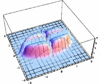
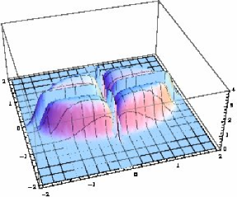
with the kernel from eq. (21), see Fig. 1. At maximal non-Hermiticity $\mu=1$ it reduces to an incomplete Bessel-$I$ function times the Bessel-$K$ from the weight [1]

$$R_{N}^{(\beta=2)}(z_{1})\Big{|}_{\mu=1}\ =\ K_{\nu}(N|z|)\sum_{l=0}^{N-1}\frac{N^{2}}{\pi(l+\nu)!l!}\left(\frac{N|z|}{2}\right)^{2l+\nu}\ .$$ (25)

For more details about correlations functions including $N_{f}$ characteristic polynomials we refer to [32, 1].

For $\beta=4$ the $k$-point correlation functions are given by

$$R_{N}^{(\beta=4)}(z_{1},\ldots,z_{k})\ =\prod_{l=1}^{k}w_{\nu}^{(\beta=4)}(z_{l})(z_{l}^{*}-z_{l})\ \mbox{Pf}_{i,j=1,\ldots,2k}\left[{\cal K}_{N}^{(\beta=4)}(u_{i},u_{j})\right]\ ,$$ (26)

where the arguments of the antisymmetric kernel

$${\cal K}_{N}^{(\beta=4)}(z_{1},z_{2}^{\ast})\ \equiv\ \sum_{k=0}^{N-1}\frac{1}{h_{k}^{(4)}}\left(q_{2k+1}^{(\beta=4)}(z_{1})q_{2k}^{(\beta=4)}(z_{2}^{\ast})-q_{2k+1}^{(\beta=4)}(z_{2}^{\ast})q_{2k}^{(\beta=4)}(z_{1})\right)\ ,$$ (27)

run through the set of $2k$ variables $\{u_{j}\}=\{z_{1},z_{1}^{*},\dots,z_{k},z_{k}^{*}\}$, and the Pfaffian of an antisymmetric matric of size $2k$ is given by the square root of the determinant of the matrix. The polynomials inside the kernel are given by [2] (with $q_{2k+1}^{(\beta=4)}(z)$ determined up to a constant times $q_{2k}^{(\beta=4)}(z)$)

$$q_{2k+1}^{(\beta=4)}(z) = -(2k+1)!\left(\frac{4\mu^{2}\eta_{-}}{N}\right)^{2k+1}L_{2k+1}^{2\nu}\left(\frac{Nz}{4\mu^{2}\eta_{-}}\right)\ ,$$ (28)

$$q_{2k}^{(\beta=4)}(z) = \left(\frac{8\mu^{2}\eta_{+}}{N}\right)^{2k}\sum_{j=0}^{k}\left(\frac{\eta_{-}}{\eta_{+}}\right)^{2j}\frac{k!\ (k+\nu)!(2j)!}{2^{2j}j!\ (j+\nu)!}L_{2j}^{2\nu}\left(\frac{Nz}{4\mu^{2}\eta_{-}}\right),$$

with squared norms

$$h_{k}^{(4)}\ =\ 8\pi\mu^{4}(2k+1)!\ (2k+2\nu+1)!\frac{{(1+\mu^{2})^{4k+2\nu}}}{N^{4k+2\nu+4}}\ .$$ (29)

They enjoy the following skew orthogonality conditions

$$\langle q_{2k+1}^{(4)}|q_{2l}^{(4)}\rangle_{4} = -\langle q_{2l}^{(4)}|q_{2k+1}^{(4)}\rangle_{4}\ =\ h_{k}^{(4)}\ \delta_{kl}\ ,$$

$$\langle q_{2k+1}^{(4)}|q_{2l+1}^{(4)}\rangle_{4} = \,\ \ \langle q_{2l}^{(4)}|q_{2k}^{(4)}\rangle_{4}\ \ \ \ =\ 0\ ,$$ (30)

with respect to the following skew-product

$$\langle h|g\rangle_{\beta=4}\ \equiv\ \int d^{2}z\ w_{\nu}^{(\beta=4)}(z)\ (z^{\ast}-z)[h(z)g(z)^{\ast}-h(z)^{\ast}g(z)]\ .$$ (31)

Hence they are called skew orthogonal Laguerre polynomials in the complex plane. Again we give the simplest example, the spectral density plotted in Fig. 2

$$R_{N}^{(\beta=4)}(z)\ =w_{\nu}^{(\beta=4)}(z)(z^{*}-z){\cal K}_{N}^{(\beta=4)}(z,z^{*})\ ,$$ (32)

obtained by inserting the kernel eq. (27). At maximal non-Hermiticity it reduces to [2]

$$R_{N}^{(\beta=4)}(z)\Big{|}_{\mu=1}\ = |z|^{2\nu}K_{2\nu}(N|z|)(z^{*}-z)\frac{N^{2\nu+2}}{\pi 2^{2\nu+3}}$$

$$\times\sum_{k=0}^{N-1}\sum_{j=0}^{k}\frac{k!(k+\nu)!(z^{2k+1}z^{*\,2j}\ -\ z^{2j}z^{*\,2k+1})}{(2k+2\nu+1)!(2k+1)!2^{4j}j!(j+\nu)!}.$$

Because of the prefactor the density vanishes identically along the real line, or after mapping to Dirac eigenvalues along the real and imaginary axis. For results for the correlation functions including $N_{f}$ pairwise degenerate and nondegenerate flavors we refer to [2] and [3], respectively.

For $\beta=1$ we will only give the results for the $k$-point correlation functions for even $N=2n$. They are give by [6]

$$R_{N}^{(\beta=1)}(z_{1},\ldots,z_{k})={\mbox{Pf}}\left[\begin{array}[]{cc}{\cal K}_{N}(z_{i},z_{j})&-G_{N}(z_{i},z_{j})\\ G_{N}(z_{j},z_{i})&-W_{N}(z_{i},z_{j})\end{array}\right]_{1\leq i,j\leq k}.$$ (36)

In addition to the antisymmetric weight eq. (2) we have introduced the following two functions of two complex variables

$$G_{N}(z_{1},z_{2}) = -\int_{\mathbb{C}}d^{2}z\,{\cal K}_{N}^{(\beta=1)}(z_{1},z){F_{\nu}}(z,z_{2})\ ,$$ (37)

$$W_{N}(z_{1},z_{2}) = -{F_{\nu}}(z_{1},z_{2})+\int_{\mathbb{C}}d^{2}z\int_{\mathbb{C}}d^{2}z^{\prime}{F_{\nu}}(z_{1},z){\cal K}_{N}^{(\beta=1)}(z,z^{\prime}){F_{\nu}}(z^{\prime},z_{2})\ .$$

These are given in terms of the integrals of the antisymmetric kernel [4]

$${\cal K}_{N}^{(\beta=1)}(z_{1},z_{2}) = \frac{\eta_{-}N^{\nu}}{4\pi(8\mu^{2}\eta_{+})^{\nu+1}}\sum_{j=0}^{N-2}\left(\frac{\eta_{-}}{\eta_{+}}\right)^{2j}\!\frac{(j+1)!}{(j+\nu)!}$$

$$\times \left\{L_{j+1}^{\nu}\Big{(}\frac{Nz_{2}}{8\mu^{2}\eta_{-}}\Big{)}L_{j}^{\nu}\Big{(}\frac{Nz_{1}}{8\mu^{2}\eta_{-}}\Big{)}-(z_{1}\leftrightarrow z_{2})\right\}.$$

For odd $N$ the corresponding results can be obtained for example by the limiting procedure proposed in [16], or by following [35].

The above kernel can be expressed in terms of the following skew orthogonal polynomials [8]

$$q_{2k}^{(\beta=1)}(z) = +C_{2k}^{\nu}(z),$$ (39)

$$q_{2k+1}^{(\beta=1)}(z) = -C_{2k+1}^{\nu}(z)+N^{-2}(1+\mu^{2})^{2}\,(2k)(2k+\nu)C_{2k-1}^{\nu}(z)+c^{\prime}C_{2k}^{\nu}(z)\ ,$$

giving the skew-orthogonal Laguerre polynomials up to an arbitrary constant $c^{\prime}$. Here we have defined

$$C_{k}^{\nu}(z) \equiv \left(\frac{8\mu^{2}\eta_{-}}{N}\right)^{k}\,k!\,L_{k}^{\nu}\left(\frac{Nz}{8\mu^{2}\eta_{-}}\right)\ .$$ (40)

The corresponding skew-product is defined as

$$\langle f|g\rangle_{\beta=1}=-\langle g|f\rangle_{\beta=1}\equiv\int d^{\,2}z_{1}\,d^{\,2}z_{2}\,F_{\nu}(z_{1},z_{2})\det\left[\begin{array}[]{cc}f(z_{1})&g(z_{1})\\ f(z_{2})&g(z_{2})\end{array}\right],$$ (41)

for two functions $f(z)$ and $g(z)$ that are integrable with respect to the weight functions contained in $F_{\nu}(z_{1},z_{2})$ in eq. (2). Our skew-orthogonal polynomials defined above then satisfy

$$\langle q_{2k}^{(1)}|q_{2l+1}^{(1)}\rangle_{1} = \ -\ \ \langle q_{2l+1}^{(1)}|q_{2k+1}^{(1)}\rangle_{1}=\ h_{k}^{(1)}\delta_{kl}\ ,$$

$$\langle q_{2k}^{(1)}|q_{2l}^{(1)}\rangle_{1} = \langle q_{2k+1}^{(1)}|q_{2l+1}^{(1)}\rangle_{1}\ =\ 0\ \forall k,l\geq 0\ ,$$ (42)

where the $h_{k}^{(1)}>0$ are their positive (squared skew) norms

$$h_{k}^{(1)}\equiv 8\pi(4\mu^{2})(2k)!\,(2k+\nu)!\,(8\mu^{2}\eta_{+}/N)^{4k+\nu+1}\ .$$ (43)

The kernel is then reading

$${\cal K}_{N=2n}^{(\beta=1)}(z_{1},z_{2})=\sum_{k=0}^{n-1}\,\frac{1}{h_{k}^{(1)}}\,\big{(}q_{2k+1}^{(1)}(z_{1})q_{2k}^{(1)}(z_{2})-q_{2k+1}^{(1)}(z_{2})q_{2k}^{(1)}(z_{1})\big{)},$$ (44)

leading to eq. (3).

As already mentioned, here the $k$-point function in eq. (18) is the sum of all possible combinations of complex and real eigenvalues, starting from only complex to only real eigenvalues. For example for the spectral density plotted in Fig. 3 we have [6]

$$R_{N}^{(1)}(z)=\int_{\mathbb{C}}d^{2}z^{\prime}\,{\cal K}_{N}^{\beta=1}(z^{\prime},z){F}(z,z^{\prime})\equiv R_{N,\mathbb{C}}^{(1)}(z)+\delta(y)R_{N,\mathbb{R}}^{(1)}(x)\ .$$ (45)

Here we explicitly give the result obtained after inserting the kernel (3) and integrating with respect to the two different weights eq. (16). Denoting $z=x+iy$ we get in terms of the kernel from eq. (3)

$$R_{N,\,\mathbb{C}}^{(1)}(z) = -2i(N|z|)^{\nu}e^{2N\eta_{-}x}{\mbox{sgn}}(y){\cal K}_{N}^{(1)}(z,z^{*})2\int_{0}^{\infty}\frac{dt}{t}e^{-2N^{2}\eta_{+}^{2}t(x^{2}-y^{2})-\frac{1}{4t}}$$ (46)

$$\times K_{\frac{\nu}{2}}\Big{(}2N^{2}\eta_{+}^{2}t(x^{2}+y^{2})\Big{)}{\mbox{erfc}}\left(2N\eta_{+}\sqrt{t}|y|\right),$$

$$R_{N,\,\mathbb{R}}^{(1)}(x) = 4N^{\nu}\int_{-\infty}^{\infty}dx^{\prime}{\mbox{sgn}}(x-x^{\prime})\,|xx^{\prime}|^{\frac{\nu}{2}}e^{N\eta_{-}(x+x^{\prime})}K_{\frac{\nu}{2}}(N\eta_{+}|x|)$$ (47)

$$\times K_{\frac{\nu}{2}}(N\eta_{+}|x^{\prime}|){\cal K}_{N}^{(1)}(x,x^{\prime}).$$

At maximal non-Hermiticity the kernel eq. (3) considerably simplifies [4]

$${\cal K}_{N}^{(1)}(z,z^{*})\Big{|}_{\mu=1}=\frac{1}{4\pi}\left(\frac{N}{4}\right)^{\nu+1}(z^{*}-z)\sum_{l=0}^{N-2}\frac{1}{l!\,(l+\nu)!}\left(\frac{N|z|}{2}\right)^{2l}\!.$$ (48)

Finally in the map to the Dirac picture one has to distinguish between substituting complex or real eigenvalues. For the densities we have

$$R^{(1\,\hbox to0.0pt{ /\hss}D)}_{N,\,\mathbb{C}}(z) = 4|z|^{2}R^{(1)}_{N,\,\mathbb{C}}(z^{2}),$$ (49)

$$R^{(1,\,\hbox to0.0pt{ /\hss}D)}_{N,\,\mathbb{R}}(x) = 2|x|R^{(1)}_{N,\,\mathbb{R}}(x^{2})\ ,$$ (50)

and analogous relations hold for higher $k$-point functions.

4 The large-$N$ limit: 3 classes of complex Bessel kernels

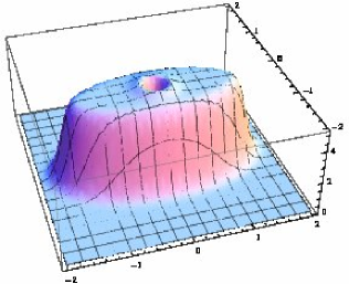
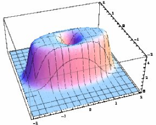
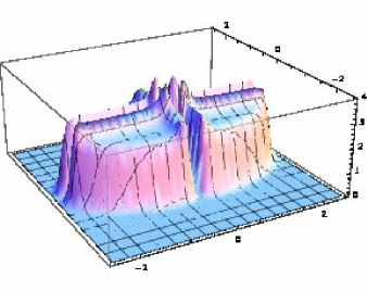
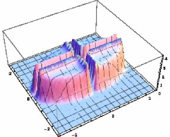
In this section we will review aspects of the large-$N$ limit for non-Hermitian Wishart random matrices. Because the eigenvalues live in the complex plane we have more possibilities in taking the large-$N$ limit, depending on the location in the spectrum. In order to illustrate where such regions are located in the complex plane we first display the so-called macroscopic (or global) limit of the spectral density. As one can see from plotting the density at finite-$N$ for all three $\beta=1,2,4$ in the Dirac picture in Figs. 1 to 3, the global spectral density follows the elliptic law [22] as their Ginibre counterparts. On top of being constant on an ellipse, various inner and outer edges exist when zooming into particular regions. This is in contrast to the real density of Wishart matrices where one can only distinguish the (soft) edge, the bulk and the origin (or hard edge) region.

In addition to the location of the spectrum two different large-$N$ limits have to be distinguished for complex eigenvalues, that of strong and weak non-Hermiticity [19]. While in the former the eigenvalues fill a two-dimensional support, in the latter they only locally extend into the complex plane. The weakly non-Hermitian limit turns out to be a one-parameter deformation both of the Hermitian and the strongly non-Hermitian limit. This makes it an ideal object to study the question of universality.

In the following we will focus on the microscopic limit at the origin, as this is a special feature of Wishart ensembles that their corresponding Ginibre counterparts cannot offer.

We begin once more by recalling the results for the macroscopic spectral density in Hermitian Wishart ensembles. Here two cases have to be distinguished. Taking the large-$N$ limit with $\nu={\cal O}(N)$, such that $c\equiv N/(N+\nu)<1$ one obtains the Marchenko-Pastur distribution [31] for the positive Wishart eigenvalues for all three values of $\beta$

$$\rho^{(\beta,M\!P)}(\lambda)=\frac{1}{2\pi c\lambda}\sqrt{(\lambda-cX_{-})(cX_{+}-\lambda)}\ ,\ \ X_{\pm}\equiv\sqrt{c^{-1/2}\pm 1}$$ (51)

on $\lambda\in[cX_{-},cX_{+}]$ and zero outside. For asymptotically square matrices with $\nu={\cal O}(1)$ at large-$N$ (leading to $c=1$) it reduces to

$$\rho^{(\beta,M\!P)}(\lambda)=\frac{1}{2\pi}\sqrt{\frac{4}{\lambda}-1}\ \Rightarrow\ \ \rho^{(\beta,\hbox to0.0pt{ /\hss}D)}(\lambda)=2|\lambda|\rho^{(\beta,M\!P)}(\lambda^{2})=\frac{1}{\pi}\sqrt{4-\lambda^{2}},$$ (52)

which is just the semi-circle after mapping to the Dirac picture. While in the Wishart picture we have a square root singularity at the origin, the density in the Dirac picture is regular at the origin.

The same phenomenon happens in the complex plane. The semi-circle density becomes replaced by the elliptic law, a constant density of an ellipse [22], which we state for the elliptic Ginibre ensemble eq. (9) (see e.g. [20]) in variables $z=x+iy$

$$\rho^{(Gin)}(z)=\frac{(1+v^{2})^{2}}{4\pi v^{2}}\ \ \mbox{for}\ \ \frac{x^{2}}{4}(1+v^{2})^{2}+\frac{y^{2}}{4v^{2}}(1+v^{2})^{2}\leq 1,$$ (53)

and zero outside. Away from the origin the mean spectral density of our three non-Hermitian Wishart ensembles is constant on an ellipse in the Dirac picture, just as its non-chiral counter parts. This can be seen in the figures below Fig. 1 - 3, where we plot the corresponding spectral densities after mapping to the Dirac picture according to eq. (49) (and eq. (50) for $\beta=1$).

Figure 1: The Dirac spectral density $R_{N}^{(\beta=2,\,\hbox to0.0pt{ /\hss}D)}(z)$ for $\beta=2$ from eq. (24) for $N=10$, $\mu=0.7$ and $\nu=0$ (left), and $\nu=1$ (right). The extra repulsion from the origin through the zero-eigenvalue at $\nu=1$ is clearly visible. In the large-$N$ limit the detailed structure at the origin will only be visible on a microscopic scale.

Figure 2: The Dirac spectral density $R_{N}^{(\beta=4,\,\hbox to0.0pt{ /\hss}D)}(z)$ for $\beta=4$ from eq. (32) for $N=20$, $\mu=0.7$ and $\nu=0$ (left) and $\nu=1$ (right). In order to see a smoother plateau we have increased $N$ here. The extra repulsion from the origin for $\nu=1$ is less pronounced here compared to $\beta=2$.

Figure 3: For $\beta=1$ we show two Dirac spectral densities: $R_{N,\mathbb{C}}^{(\beta=1,\,\hbox to0.0pt{ /\hss}D)}(z)$ for the complex eigenvalues, and $R_{N,(i)\mathbb{R}}^{(\beta=1,\,\hbox to0.0pt{ /\hss}D)}(z=x)$ $((iy))$ for the real (or purely imaginary) eigenvalues from eqs. (46) and (47). The parameter values are the same as for $\beta=4$ in Fig. 2. It is clearly visible that the density of complex eigenvalues is repelled from the real and imaginary axis as for $\beta=4$, with an apparently different profile though.

When mapping back to the Wishart picture using eq. (49) we obtain a linear decay inside the support, as was observed in [26, 12]:

$$\rho^{(\beta,\,\hbox to0.0pt{ /\hss}D)}(z)\sim const.\ \ \Rightarrow\ \ \rho^{(\beta)}(z)\sim\frac{const.}{|z|}\ .$$ (54)

Likewise the behavior at the origin, that was found to be constant for $\nu>0$ and logarithmically divergent $\sim\log|z|$ for $\nu=0$ in the Wishart picture [26], gets bent to zero in the Dirac picture using the map eq. (49). This can bee seen in the figures for all three $\beta$ and the values of $\nu=0,1$.

In addition, in [26, 12] the limit $\nu={\cal O}(N)$, such that $q\equiv\nu/N>0$ is finite, was performed for $\beta=2$ at $\mu=1$, leading to the density

$$\rho^{(\beta=2)}(z)=\frac{1}{4\pi\sqrt{|z|^{2}+q^{2}}}\ ,$$ (55)

on the support, which we give in the Wishart picture here. This is the generalization of the Marchenko-Pastur distribution eq. (51) into the complex plane.

Let us now turn to the microscopic large-$N$ limit. As can be seen from the figures several regions could be investigated by zooming into the outer edges or inner edges along the axes. However, in the following we will restrict ourselves to the microscopic origin limit, as this limit is particular to the Wishart ensembles.

We begin with the microscopic origin limit at strong non-Hermiticity $(S)$. Because strong and maximal non-Hermiticity at $\mu=1$ are related by a simple rescaling of the complex eigenvalues, $z\to 2\eta_{+}z$ (see e.g. [20, 6]), we restrict ourselves only to the latter. This limit is defined such that the non-Hermiticity parameter $\mu$ is not scaled with $N$, only the complex eigenvalues get rescaled:

$$\rho^{(\beta,\,\hbox to0.0pt{ /\hss}D)}_{S}(\xi)\ \equiv\ \lim_{N\to\infty}\frac{1}{N}R_{N}^{(\beta,\,\hbox to0.0pt{ /\hss}D)}\left(z=\xi/\sqrt{N}\right)\ ,\ \ \lim_{N\to\infty}\sqrt{N}z=\xi\ \ \mbox{fixed},$$ (56)

and all higher order correlation functions are rescaled accordingly.

For $\beta=2$ we obtain easily from eq. (25) [1]

$$\rho^{(\beta,\,\hbox to0.0pt{ /\hss}D)}_{S}(\xi)\ =\ \frac{2}{\pi}|\xi|^{2}K_{\nu}(|\xi|^{2})I_{\nu}(|\xi|^{2})\stackrel{{\scriptstyle|\xi|\to\infty}}{{\longrightarrow}}\frac{1}{\pi}\ .$$ (57)

It only depends on the rescaled modulus $|\xi|$ and is thus rotationally invariant. We also give the asymptotic value of the microscopic density that matches the constant value of the macroscopic density in the Dirac picture.

For $\beta=4$ we obtain from eq. (3) after a non-trivial calculation [2]

$$\rho^{(4,\,\hbox to0.0pt{ /\hss}D)}_{S}(\xi) = \frac{|\xi|^{2}}{4\pi}(\xi^{\ast\,2}-\xi^{2})K_{2\nu}\left({|\xi|^{2}}\right)$$

$$\times\int_{0}^{1}du\frac{I_{2\nu}(u|\xi|^{2})}{\sqrt{1-u^{2}}}\sinh\left(\frac{\sqrt{1-u^{2}}}{2}(\xi^{2}-\xi^{\ast\,2})\right).$$

Compared to $\beta=2$ the density is no longer rotationally invariant, reflecting the repulsion of the complex eigenvalues from real and imaginary axes.

For $\beta=1$ we obtain two densities from eqs. (46) and (47), for the complex eigenvalues and the eigenvalues on the real and imaginary axis [6]:

$$\rho_{\mathbb{C},S}^{(1,\,\hbox to0.0pt{ /\hss}D)}(\xi) = {\mbox{sgn}}(\Im m(\xi^{2}))(-i)(\xi^{2}-\xi^{*\,2})\frac{8}{\pi}|\xi|^{2}I_{\nu}\left(2|\xi|^{2}\right)$$ (59)

$$\times\int_{0}^{\infty}\frac{dt}{t}\,e^{-(\xi^{4}+\xi^{*\,4}){t}-\frac{1}{4t}}\,K_{\frac{\nu}{2}}\left(2{|\xi|^{4}t}\right){\mbox{erfc}}\left(2\sqrt{t}\,|\Im m(\xi^{2})|\right)\!,\ \ \ \ \ \$$

$$\rho_{(i)\mathbb{R}\,S}^{(1,\,\hbox to0.0pt{ /\hss}D)}(\xi) = \frac{1}{\pi}|\xi|\,K_{\frac{\nu}{2}}(|\xi|^{2})\left(\int_{0}^{\infty}dx^{\prime}\,|\xi^{2}-x^{\prime}|\ K_{\frac{\nu}{2}}(|x^{\prime}|)\ I_{\nu}(2\xi\sqrt{x^{\prime}})\right.$$ (60)

$$\left.+\int_{-\infty}^{0}dx^{\prime}\,|\xi^{2}-x^{\prime}|\ K_{\frac{\nu}{2}}(|x^{\prime}|)\ J_{\nu}(2\xi\sqrt{|x^{\prime}|})\right),$$

where in the second equation $\xi\in{\mathbb{R}}$ (or $\xi\in i{\mathbb{R}}$ which is identical here). Once again the density in the complex plane is not rotationally invariant, and vanishes along the real and imaginary axis.

We now turn to the microscopic origin limit as weak non-Hermiticity $(W)$ first introduced for the Ginibre ensembles eq. (9) in [19]. It is defined by both rescaling $\mu$ with $N$, as well as the complex eigenvalues (with a different power compared to the strong limit above):

$$\rho^{(\beta,\,\hbox to0.0pt{ /\hss}D)}_{W}(\xi)\ \equiv\ \lim_{N\to\infty}\frac{1}{N^{2}}R_{N}^{(\beta,\,\hbox to0.0pt{ /\hss}D)}\left(z=\xi/{N}\right)\ ,$$ (61)

with

$$\lim_{N\to\infty}2{N^{2}}\mu^{2}=\alpha^{2}\$$ (62)

fixed. All higher order correlation functions are rescaled accordingly.

For $\beta=2$ we get [32]

$$\rho_{W}^{(2,\,\hbox to0.0pt{ /\hss}D)}(\xi) = \frac{1}{2\pi\alpha^{2}}|\xi|^{2}K_{\nu}\left(\frac{|\xi|^{2}}{4\alpha^{2}}\right)e^{\frac{\xi^{2}+\xi^{*\,2}}{8\alpha^{2}}}\int_{0}^{1}dt\,t\,e^{-2\alpha^{2}t^{2}}J_{\nu}(t\xi)J_{\nu}(t\xi^{*})$$ (63)

$$\stackrel{{\scriptstyle\alpha\to 0}}{{\longrightarrow}} \delta(\Im m\xi)\frac{1}{2}(J_{\nu}(\xi)^{2}-J_{\nu-1}(\xi)J_{\nu+1}(\xi))\ .$$

It agrees with the density obtained from a non-Hermitian one-matrix model [26]. In the second line we indicate that in the Hermitian limit $\alpha\to 0$ the density reduces to the known universal Bessel density times a delta function in the imaginary part. In the opposite limit $\alpha\to\infty$ the density at strong non-Hermiticity given in eq. (57) can be recovered, and we refer to [1] for more details.

For $\beta=4$ the weak non-Hermiticity limit yields [2]

$$\rho_{W}^{(4,\,\hbox to0.0pt{ /\hss}D)}(\xi) = \frac{|\xi|^{2}}{32\alpha^{4}}(\xi^{\ast\,2}-\xi^{2})K_{2\nu}\left(\frac{|\xi|^{2}}{2\alpha^{2}}\right)e^{\frac{(\xi^{2}+\xi^{*\,2})}{4\alpha^{2}}}\int_{0}^{1}ds\int_{0}^{1}\frac{dt}{\sqrt{t}}{e}^{-2s(1+t)\alpha^{2}}$$ (64)

$$\times\Big{[}J_{2\nu}(2\sqrt{st}\xi)J_{2\nu}(2\sqrt{s}\xi^{\ast})-J_{2\nu}(2\sqrt{s}\xi)J_{2\nu}(2\sqrt{st}\xi^{\ast})\Big{]}.$$

Once again in the Hermitian limit $\alpha\to 0$ the prefactor in front of the integral reduces to a delta function in $\Im m(\xi)$, and the integral matches the known universal Bessel kernel for $\beta=4$ (which also has a simpler representation expressed in terms of the $\beta=2$ density plus a single integral).

Finally we give the weak origin limit for $\beta=1$ which was obtained most recently. The complication arises from the fact that for the real eigenvalues both at $\mu=0$ in the real Wishart ensemble, and at $\mu\neq 0$ for our non-Hermitian extension, the large-$N$ limit of the kernel and the integration in eq. (47) do not commute. For more details we refer to [9, 34] and only quote the answer valid for $\xi\in\mathbb{R}$ and $\xi\in i\mathbb{R}$

$$\rho_{(i)\mathbb{R},W}^{(1,\,\hbox to0.0pt{ /\hss}D)}(\xi) = \frac{2|\xi|h_{w}(\xi^{2})}{[{\mbox{sgn}}\xi^{2}]^{\frac{\nu}{2}}}\Bigg{\{}\!\!\left((-i)^{\nu}\int_{-\infty}^{0}dy+\int_{0}^{\xi^{2}}\frac{2dy}{[{\mbox{sgn}}\xi^{2}]^{\frac{\nu}{2}}}\right){\cal K}_{w}(\xi^{2},y)h_{w}(y)$$

$$-\frac{1}{32\sqrt{\pi}}\Bigg{[}-\,\frac{1}{\sqrt{2}\alpha}\,\e^{-2\alpha^{2}}\,J_{\nu}(\xi)+\frac{2(\sqrt{2}\alpha)^{\nu}}{\Gamma\left(\frac{\nu+1}{2}\right)}\,\int_{0}^{1}ds\,\e^{-2\alpha^{2}s^{2}}s^{\nu+2}$$

$$\times\!\left(\frac{\xi}{2}\,E_{-}(s)\,J_{\nu+1}(s\xi)-2\alpha^{2}s\left(E_{+}(s)-E_{-}(s)\right)J_{\nu}(s\xi)\right)\!\!\Bigg{]}\!\Bigg{\}},$$

where we have defined the kernel in the weak limit

$${\cal K}_{W}^{(1)}(\xi,\xi^{*})\equiv\int_{0}^{1}\frac{ds\,s^{2}}{2^{9}\pi\alpha^{2}}e^{-4\alpha^{2}s^{2}}\Big{(}\xi J_{\nu+1}(s\xi)J_{\nu}(s\xi^{*})-\xi^{*}J_{\nu+1}(s\xi^{*})J_{\nu}(s\xi)\Big{)},$$ (66)

the rescaled real weight function

$$h_{w}(\xi^{2})\equiv\frac{2}{\xi^{\nu}}e^{\xi^{2}/16\alpha^{2}}\,2K_{\frac{\nu}{2}}\left(\frac{|\xi|^{2}}{16\alpha^{2}}\right)\ ,$$ (67)

and the exponential integral

$$E_{\mp}(s)\equiv\int_{1}^{\infty}dt\,t^{\frac{\nu}{2}\mp\frac{1}{2}}\,e^{-2\alpha^{2}s^{2}t}\,.$$ (68)

The weak density of complex eigenvalues presents no such difficulties [6]:

$$\rho_{\mathbb{C},W}^{(1,\,\hbox to0.0pt{ /\hss}D)}(\xi) = -16i|\xi|^{2}{\mbox{sgn}}({\Im\mbox{m}}\,\xi^{2})e^{\frac{1}{8\alpha^{2}}(\xi^{2}+\xi^{*\,2})}{\cal K}_{W}^{(1)}(\xi,\xi^{*})$$

$$\times\int_{0}^{\infty}\frac{dt}{t}e^{-\frac{t}{2^{8}\alpha^{4}}(\xi^{4}+\xi^{*\,4})-\frac{1}{4t}}K_{\frac{\nu}{2}}\!\left(\frac{t}{2^{7}\alpha^{4}}|\xi|^{4}\right){\mbox{erfc}}\Big{(}\frac{\sqrt{t}}{8\alpha^{2}}|{\Im\mbox{m}}(\xi^{2})|\Big{)}.$$

In the Hermitian limit $\alpha\to 0$ the density of complex eigenvalues as well as the density along the imaginary axis vanishes. Only the density of real eigenvalues will build up the known density of real eigenvalues in the Hermitian Wishart ensemble for $\beta=1$ [6].

5 Conclusions

In this short article we have reviewed the solution of three non-Hermitian extensions of Wishart ensembles of random matrices with real, complex or quaternion real elements. In all three cases the eigenvalue correlation functions are expressed in terms of the kernel of (skew) orthogonal Laguerre polynomials in the complex plane, depending on a non-Hermiticity parameter that allows to interpolate between Wishart and maximally non-Hermitian Wishart ensembles, for finite and infinite $N$. At the origin these ensembles are very well understood, and we gave the corresponding three Bessel kernels in the complex plane at strong and weak non-Hermiticity. At the various inner and outer edges we expect that the behavior of the corresponding Ginibre ensembles (see e.g. in [27]), and the ensembles we considered here is be the same and thus universal. This was shown for example in [7] for the generalized Airy kernel at the soft edge along the real line, or in [26] in the rotationally invariant case (regime II (iii)) at the outer edge, both for $\beta=2$. The latter behavior was also found for the outer edge density of random contractions [27].

At present a deeper guiding principle to prove universality for non-Hermitian random matrices with a larger class of weight functions, such as quasiharmonic potentials [39] is lacking. A first step towards universality could be to show that different Gaussian models lead to the same answer as mentioned above, or as it was shown in yet another example for the Bessel kernel in the weak limit at $\beta=2$ eq. (63), starting from a Gaussian one- or two-matrix model in [36] and [32], respectively. We hope that these first steps will ultimately lead to a deeper understanding of the issue of universality.

Acknowledgments I would like to thank all my coworkers for collaborations on this subject, as well as the organizers of this workshop for the very stimulating atmosphere.

References

• [1] G. Akemann, J.C. Osborn, K. Splittorff and J.J.M. Verbaarschot, Nucl. Phys. B712 (2005) 287 [hep-th/0411030].
• [2] G. Akemann, Nucl. Phys. B730 (2005) 253 [hep-th/0507156].
• [3] G. Akemann and F. Basile, Nucl. Phys. B766 (2007) 150 [arXiv:math-ph/0606060].
• [4] G. Akemann, M.J. Phillips and H.-J. Sommers, J. Phys. A: Math. Theor. 42 (2009) 012001 [arXiv:0810.1458v1 [math-ph]].
• [5] G. Akemann, M.J. Phillips and L. Shifrin, J. Math. Phys. 50 (2009) 063504 [arXiv:0901.0897v2 [math-ph]].
• [6] G. Akemann, M. J. Phillips and H. J. Sommers, J. Phys. A43 (2010) 085211 [arXiv:0911.1276 [hep-th]].
• [7] G. Akemann and M. Bender, J. Math. Phys.  51 (2010) 103524 [arXiv:1003.4222 [math-ph]].
• [8] G. Akemann, M. Kieburg and M. J. Phillips, J. Phys. A43 (2010) 375207 [arXiv:1005.2983 [math-ph]].
• [9] G. Akemann, T. Kanazawa, M. J. Phillips and T. Wettig, JHEP 1103 (2011) 066 [arXiv:1012.4461 [hep-lat]].
• [10] D. Bernard and A. LeClair, A Classification of Non-Hermitian Random Matrices, proceedings of the NATO Advanced Research Workshop on “Statistical Field Theories”, Como 18-23 June 2001 [arXiv:cond-mat/0110649].
• [11] C. Biely and S. Thurner, Quant. Finance 8 (2008) 705 [arXiv:physics/0609053v1 [physics.soc-ph]].
• [12] Z. Burda, A. Jarosz, G. Livan, M. A. Nowak and A. Swiech, Phys. Rev. E82 (2010) 061114 arXiv:1007.3594v1 [cond-mat.stat-mech].
• [13] Z. Burda, A. Jarosz, G. Livan, M. A. Nowak and A. Swiech, arXiv:1103.3964v1 [cond-mat.stat-mech].
• [14] A. Crisanti, G. Paladin and A. Vulpiani, Products of Random Matrices in Statistical Physics, Springer, Berlin (1993).
• [15] P.J. Forrester and T. Nagao, Phys. Rev. Lett. 99 050603 (2007) [arXiv:0706.2020 [cond-mat.stat-mech]]; J. Phys. A41, 375003 (2008) [arXiv:0806.0055 [math-ph]].
• [16] P.J. Forrester and A. Mays, J. Stat. Phys. 134 (2009) 443 [arXiv:0809.5116v2 [math-ph]].
• [17] P.J. Forrester and A. Mays, arXiv:0910.2531v2 [math-ph].
• [18] P.J. Forrester, Log-Gases and Random Matrices, London Mathematical Society Monographs no. 34, Princeton University Press, Princeton (2010).
• [19] Y.V. Fyodorov, B.A. Khoruzhenko, and H.-J. Sommers, Phys. Lett. A226 (1997) 46 [arXiv:cond-mat/9606173]; Phys. Rev. Lett. 79 (1997) 557 [arXiv:cond-mat/9703152].
• [20] Y.V. Fyodorov, B.A. Khoruzhenko and H.-J. Sommers, Ann. Inst. Henri Poincaré 68 (1998) 449 [arXiv:chao-dyn/9802025].
• [21] J. Ginibre, J. Math. Phys. 6 (1965) 440.
• [22] V.L. Girko, Theor. Prob. Appl. 30 (1986) 677.
• [23] M.A. Halasz, J.C. Osborn and J.J.M. Verbaarschot, Phys. Rev. D56 (1997) 7059 [hep-lat/9704007].
• [24] T. Kanazawa, T. Wettig and N. Yamamoto, Phys. Rev. D81 (2010) 081701 [arXiv:0912.4999 [hep-ph]].
• [25] E. Kanzieper, J. Phys. A: Math. Gen. 35 (2002) 6631 [cond-mat/0109287].
• [26] E. Kanzieper and N. Singh, J. Math. Phys. 51 (2010) 103510 [arXiv:1006.3096v2 [math-ph]].
• [27] B.A. Khoruzhenko and H.-J. Sommers, “Non-Hermitian Random Matrix Ensembles”, invited chapter in “Handbook of Random Matrix Theory”, Eds. G. Akemann, J. Baik, P. Di Francesco, Oxford University Press 2011 [arXiv:0911.5645[math-ph]].
• [28] J. Kwapień, S. Drożdż, and A. A. Ioannides, Phys. Rev. E62 (2000) 5557 [arXiv:cond-mat/0002175v1 [cond-mat.stat-mech].
• [29] J. Kwapień, S. Drożdż, A.Z. Górski and P. Oświecimka, Acta Phys. Pol. B37 (2006) 3039 [arXiv:physics/0605115v1 [physics.soc-ph]].
• [30] U. Magnea, J. Phys. A41 (2008) 045203 [arXiv:0707.0418v2 [math-ph]].
• [31] V.A. Marchenko and L.A. Pastur, Math. USSR-Sb, 1 (1967) 457.
• [32] J.C. Osborn, Phys. Rev. Lett. 93 (2004) 222001 [hep-th/0403131].
• [33] K.A. Penson, K. Życzkowski, arXiv:1103.3453v2 [math-ph].
• [34] M.J. Phillips, PhD thesis, Brunel University West London, 2011.
• [35] H.-J. Sommers and W. Wieczorek, J. Phys. A41 (2008) 405003 [arXiv:0806.2756 [cond-mat.stat-mech]].
• [36] K. Splittorff and J.J.M. Verbaarschot, Nucl. Phys. B683 (2004) 467 [arXiv:hep-th/0310271v3].
• [37] M. Stephanov, Phys. Rev. Lett. 76 (1996) 4472 [hep-lat/9604003].
• [38] J.J.M. Verbaarschot, “Handbook Article on Applications of Random Matrix Theory to QCD,” invited chapter in ”Handbook of Random Matrix Theory”, Eds. G. Akemann, J. Baik, P. Di Francesco, Oxford University Press 2011 [arXiv:0910.4134 [hep-th]].
• [39] A. Zabrodin, ”Random matrices and Laplacian growth”, invited chapter in ”Handbook of Random Matrix Theory”, Eds. G. Akemann, J. Baik, P. Di Francesco, Oxford University Press 2011 [arXiv:0907.4929v1 [math-ph]].