OGLE-2005-BLG-018: Characterization of Full Physical and Orbital Parameters of a Gravitational Binary Lens

Abstract

We present the analysis result of a gravitational binary-lensing event OGLE-2005-BLG-018. The light curve of the event is characterized by 2 adjacent strong features and a single weak feature separated from the strong features. The light curve exhibits noticeable deviations from the best-fit model based on standard binary parameters. To explain the deviation, we test models including various higher-order effects of the motions of the observer, source, and lens. From this, we find that it is necessary to account for the orbital motion of the lens in describing the light curve. From modeling of the light curve considering the parallax effect and Keplerian orbital motion, we are able to measure not only the physical parameters but also a complete orbital solution of the lens system. It is found that the event was produced by a binary lens located in the Galactic bulge with a distance $6.7\pm 0.3$ kpc from the Earth. The individual lens components with masses $0.9\pm 0.3\ M_{\odot}$ and $0.5\pm 0.1\ M_{\odot}$ are separated with a semi-major axis of $a=2.5\pm 1.0$ AU and orbiting each other with a period $P=3.1\pm 1.3$ yr. The event demonstrates that it is possible to extract detailed information about binary lens systems from well-resolved lensing light curves.

1 Introduction

Microlensing occurs when an astronomical object approaches close to the line of sight toward a background star. Due to the gravity of the intervening object (lens), light rays from the background star (source) bend, causing splits and distortions of the source star image. For Galactic microlensing events, the separation between the split images is an order of milli-arcsec and thus it is difficult to directly observe the split images. However, the lensing phenomenon can be observed by the change of the source star brightness. For a point-source single-lens event, the magnification of the source star flux is represented by (Paczyński, 1986)

$$A={u^{2}+2\over u(u^{2}+4)^{1/2}};\qquad u=\left[\left({t-t_{0}\over t_{\rm E}}\right)^{2}+u_{0}^{2}\right]^{1/2},$$ (1)

where $u$ is the lens-source separation in unit of the angular Einstein radius $\theta_{\rm E}$, $t_{0}$ is the time of closest lens-source approach, $u_{0}$ is the lens-source separation at that moment, and $t_{\rm E}$ is the time required for the source to transit $\theta_{\rm E}$ (Einstein time scale). The Einstein radius is related to the physical parameters of the lens system by

$$\theta_{\rm E}=(\kappa M\pi_{\rm rel})^{1/2},$$ (2)

where $\kappa=4G/(c^{2}\rm AU)$, $M$ is the mass of the lens, $\pi_{\rm rel}={\rm AU}(D_{\rm L}^{-1}-D_{\rm S}^{-1})$, and $D_{\rm L}$ and $D_{\rm S}$ are the distances to the lens and source, respectively. A standard single-lens event is characterized by a non-repeating, smooth, and symmetric light curve and modeling it requires 3 parameters of $t_{0}$, $u_{0}$, and $t_{\rm E}$. Since the first detections by Alcock et al. (1993) and Udalski et al. (1993), microlensing events have been detected toward various star fields including the Galactic bulge (Udalski et al., 2005; Sumi et al., 2010), Large and Small Magellanic Clouds (Wyrzykowski et al., 2009, 2010), and M31 (Calchi Novati et al., 2010). Currently, events are being detected with a rate of more than 500 events per year, mostly toward the bulge field.

Among lensing events, a fraction of events are produced by lenses composed of two masses. These binary-lens events can exhibit light curves that are dramatically different from those of single-lens events (Mao & Paczyński, 1991). The most prominent features occur when the source closely approaches or crosses caustics, which represent the set of source positions at which the lensing magnification of a point source becomes infinity. Describing a standard binary-lens light curve requires to include three additional parameters: the mass ratio of the companion to its host, $q$, the projected separation between the lens components in units of the Einstein radius, $s_{\perp}$, and the angle between the source trajectory and the binary axis, $\alpha$. For a caustic-crossing event, an additional parameter of the source radius normalized by the Einstein radius, $\rho_{\star}$ (normalized source radius), is required to account for the finite-source effect (Domink, 1995; Gaudi & Gould, 1999; Gaudi & Petters, 2002; Pejcha & Heyrovský, 2009).

Figure 1: Light curve of the microlensing event OGLE-2005-BLG-018. Also presented our light curves from modelings based on the standard binary parameters (dotted curve) and considering the parallax and orbital effects (solid curve).

However, modeling binary-lens light curves with the standard parameters is occasionally not adequate to precisely describe light curves. This is because light curves are subject to various higher-order effects that result in deviations from the canonical form. The causes of these effects include the motions of the observer, source, and lens during the event. The change of the observer’s position induced by the orbital motion of the Earth around the Sun causes the source motion with respect to the lens to deviate from rectilinear, and thus the resulting light curve can exhibit long-term deviations. This is known as the “parallax” effect (Gould, 1992; Refsdal, 1966). If the source star is a binary, the source trajectory can also be affected by the orbital motion of the source over the course of the event. This is known as the “xallarap” effect (Han & Gould, 1997), i.e., reverse order of the spell of “parallax”. Finally, the binary nature of the lens implies that the positions of the lens components vary in time due to their orbital motion. This “orbital” effect causes not only the change of the source position with respect to the lens but also the magnification pattern because the projected binary separation changes in time (Dominik, 1998; Ioka et al., 1999; Albrow et al., 2000; Rattenbury et al., 2002). The deviations in lensing light curves caused by these second-order effects are usually very small and thus difficult to measure. However, when they are measured, they provide information that allows to better constrain the lens system. For example, if the deviation caused by the parallax effect is measured, it is possible to determine the physical parameters of the lens mass, distance to it, and the projected separation in physical units (Gould, 1992). If the orbital effect is measured, one can further constrain the lens system by determining the orbital parameters and intrinsic separation between the lens components (Gaudi et al., 2008; Dong et al., 2009; Bennett et al., 2010; Penny et al., 2010; Yee et al., 2010; Skowron et al., 2010).

In this paper, we analyze the light curve of the binary-lensing event OGLE-2005-BLG-018 by combining all available data obtained from survey and follow-up observations. The event was analyzed before by Skowron et al. (2007) based on the OGLE data and their model shows noticeable deviations. Our preliminary modeling also indicated that a model based on the standard binary parameters is not adequate enough to precisely describe the observed light curve, suggesting the need to consider higher-order effects. We conduct analysis of the light curve considering various second-order effects and present the constraints of the lens system obtained from modeling.

2 Observation

The event OGLE-2005-BLG-018 occurred on a Galactic bulge star located at $(\alpha,\delta)_{\rm J2000}=(17^{\rm h}51^{\rm m}23^{\rm s}\hskip-2.0pt.53,-29^{\circ}39^{\prime}22^{\prime\prime}\hskip-2.0pt.8)$, which corresponds to the Galactic coordinates $(l,b)=(0.03^{\circ},-1.45^{\circ})$. The event was detected by the Optical Gravitational Lensing Experiment (OGLE: Udalski et al., 2003) using the 1.3 m Warsaw telescope of Las Campanas Observatory in Chile. An anomaly alert was issued on 2005 Mar 31 by the OGLE group. In addition, a series of real-time models were issued by M. Dominik (2010, private communication). Following the alert and models, the event was intensively observed by follow-up groups including the Probing Lensing Anomalies Network (PLANET: Beaulieu et al., 2006), RoboNet (Tsapras et al., 2009), and Microlensing Follow-Up Network ($\mu$FUN: Gould, 2006) by using six telescopes located on four different continents. The telescopes used for follow-up observations include 2.0 m Faulkes Telescope N. (FTN) in Hawaii, 2.0 m Liverpool Telescope (LT) in La Palma, Spain, 1.0 m of Mt. Canopus Observatory in Australia, and 1.54 m Danish Telescope of La Silla Observatory in Chile, 0.6 m of Perth Observatory in Australia, and 1.3 m SMARTS telescope of CTIO in Chile. Thanks to the follow-up observations, the light curve was very densely resolved.

Figure 1 shows the light curve of the event. It is characterized by three distinctive features, occurring at ${\rm HJD}\sim 2453460\ (t_{1})$, $2453512\ (t_{2})$, and $2453528\ (t_{3})$. The two adjacent peaks at $t_{2}$ and $t_{3}$ are strong while the other peak at $t_{1}$ is relatively weak and separated from the strong features.

3 Modeling of Second-Order Effects

We first conduct modeling of the light curve with the set of standard binary parameters. As shown in Figure 1, the best-fit light curve from this initial modeling shows noticeable deviations from the observed light curve especially near the part of the light curve around the weak feature although the model light curve describes the two strong features relatively well. Investigation of the lens system geometry obtained from the standard modeling indicates that the projected separation between the binary lens components is smaller than the Einstein radius, i.e., $s_{\perp}<1$. In this case, the resulting caustics are composed of 3 segments, where one large central caustics is located around the center of mass of the binary and the other two small caustics are located away from the central caustic (Scheneider & Weiss, 1986). The model also indicates that the two strong features of the light curve were produced by two successive crossings of the source over the central caustic and the weak feature was produced by the approach to one of the two peripheral caustics. Events produced by such a lens system are susceptible to the orbital effect because the peripheral caustic moves considerably even for a small shift of the binary axis. In addition, the long duration of the event, which lasted $\sim 200$ days, raises the need to consider both the parallax and xallarap effects. We, therefore, conduct modelings of the light curve considering these second-order effects as well.

Considering the parallax effect into modeling requires to include two additional parameters of $\pi_{{\rm E},N}$ and $\pi_{{\rm E},E}$. These parameters represent the two components of the lens parallax vector $\mbox{\boldmath$\pi$}_{\rm E}$ projected on the sky in the north and east equatorial coordinates, respectively. The direction of the parallax vector corresponds to that of the lens-source relative motion in the frame of the Earth at a specific time of the event. We set the reference time at the moment of the second perturbation peak, i.e., $t_{2}$. The size of the parallax vector corresponds to the ratio of the Earth’s orbit to the Einstein radius projected on the observer observer’s plane, i.e., $\pi_{\rm E}={\rm AU}/[r_{\rm E}D_{\rm S}/(D_{\rm S}-D_{\rm L})]$.

Under the assumption of a circular orbit and a very faint binary companion, the xallarap effect is described by 5 parameters. They are the orbital period of the source, $P_{\rm S}$, inclination, $i_{\rm S}$, phase angle, $\psi$, and the two components of the xallarap vector in the north and east direction, $\xi_{{\rm E},N}$ and $\xi_{{\rm E},E}$. The magnitude of the xallarap vector $\mbox{\boldmath$\xi$}_{\rm E}$ corresponds to the ratio of the source star’s orbit to the Einstein radius projected on the source plane.

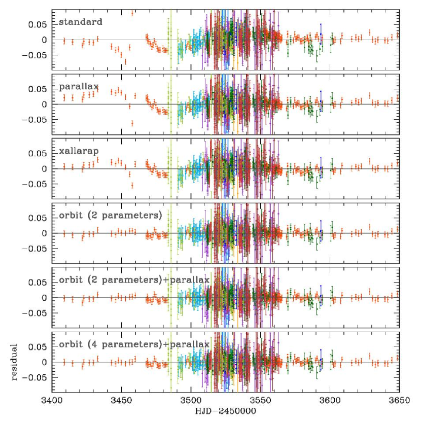
Figure 2: Residual of data from 6 different models.

To account for the orbital effect, we consider 2 types of parameterization. The first one is based on the approximation that the binary lens rotates with a constant angular speed and the projected separation between its components changes with a constant rate. This parameterization requires two parameters of $d\alpha/dt$ and $ds_{\perp}/dt$, which represent the changing rates of the angle between the binary axis and the source trajectory and the projected separation between the lens components, respectively. In the second parameterization, we fully consider the Keplerian orbital motion. This requires to include 2 extra parameters in addition to the orbital parameters used in the first type of parameterization. These additional parameters are $s_{\parallel}$ and $ds_{\parallel}/dt$, where $s_{\parallel}$ represents the line-of-sight separation between the binary components in units of $\theta_{\rm E}$ and $ds_{\parallel}/dt$ represents its rate of change. For the full description of the orbital lensing parameters, see the summary in the Appendix of Skowron et al. (2010).

With these parameterizations, we test 6 different models. The first model is based on standard binary parameters with a static lens and source and no parallax motion of the Earth (standard model). The second and third models include the parallax and xallarap effects, respectively. The fourth model includes the orbital effect of the lens with 2 parameters of $d\alpha/dt$ and $ds_{\perp}/dt$. In the last two models, we consider both the parallax and orbital effects where the orbital effect is described by 2 and 4 parameters, respectively. We note that 4-parameter orbital modeling must include the parallax parameters whereas 2-parameter orbital modeling does not necessarily needs this.

We search for the solution of the best-fit parameters of the individual models by minimizing $\chi^{2}$ in the parameter space. For binary-lensing modeling, this is a very complex procedure due to several reasons. First, the complexity of the $\chi^{2}$ surface in the parameter space makes it difficult to rule out the possibility of the existence of local minima (Dominik, 1999), implying that even if a plausible model is found, it is difficult to be sure the solution is the correct one. This makes it difficult to use a simple downhill approach to search for solutions. Second, modeling is further complicated by the sheer size of the parameter space. The large number of parameters implies that brute-force searches for solutions are very difficult and extremely time-consuming. To resolve the degeneracy problem but avoiding searches throughout all parameter space, we use a hybrid approach in which grid searches are conducted over the space of a set of parameters and the remaining parameters are searched by using a downhill approach. We choose $s_{\perp}$, $q$, and $\alpha$ as the grid parameters because they are related to the light curve features in a complex way such that a small change in the values of the parameters can lead to dramatic changes in the resulting light curve. On the other hand, the other parameters are more directly related to the light curve features and thus they can be searched for by using a downhill approach. For the $\chi^{2}$ minimization in the downhill approach, we use the Markov Chain Monte Carlo (MCMC) method.

Another difficulty in binary-lensing modeling arises due to large computation. Most binary-lens events exhibit perturbations induced by caustic crossings or approaches during which the finite-source effect is important. Calculating finite magnifications involves a numerical method, which requires heavy computations. Considering that modeling requires to produce a large number of light curves of trial models, it is important to apply an efficient method for magnification calculations. We accelerate the computation first by minimizing computations in the numerical method and second by restricting the numerical computation only when it is necessary. The numerical method applied for finite magnification computations is based on the ray-shooting method. In this method, a large number of rays are uniformly shot from the image plane, bent according to the lens equation, land on the source plane, and then the magnification is computed as the ratio of the number density of rays on the source surface to the density on the image plane. In this process, we reduce the number of rays required for magnification computations by shooting only ones arriving at the region around the caustics. We further restrict numerical computations by applying a simple analytic hexadecapole approximation for finite magnifications (Pejcha & Heyrovský, 2009; Gould, 2008) unless the source is located very close to the caustics.

We incorporate the effect of the limb-darkening of the source star surface when we compute the finite-source magnification. The surface brightness is modeled by

$$S_{\lambda}={F_{\lambda}\over\pi\theta_{\star}^{2}}\left[1-\Gamma_{\lambda}\left(1-{3\over 2}\cos\theta\right)\right],$$ (3)

where $\Gamma_{\lambda}$ is the linear limb-darkening coefficients, $F_{\lambda}$ is the flux, and $\theta$ is the angle between the normal to the source star’s surface and the line of sight toward the star. From the color of the source star measured from the location on the color-magnitude diagram, it is found that the source is a clump giant. We, therefore, use the limb-darkening coefficients of $\Gamma_{V}=0.708$, $\Gamma_{I}=0.613$, and $\Gamma_{R}=0.508$ by adopting the values from Claret (2000) under the assumption that $v_{\rm turb}=2\ {\rm km}\ {\rm s}^{-1}$, $\log(g/g_{\odot})=-1.9$, and $T_{\rm eff}=4750$ K.

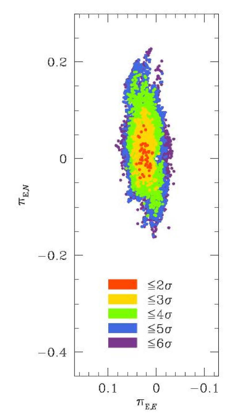
Figure 3: Scatter plot of Markov chains in the space of the parallax parameters $\pi_{{\rm E},E}$ and $\pi_{{\rm E},N}$ for the best-fit model. Different colors of points represent $\Delta\chi^{2}$ from the minimum.

Figure 4: Histograms of lens orbital parameters obtained from the 4-parameter orbital fit.

4 Result

In Table 1, we present the solutions found for the 6 tested models. In Figure 2, we also present the residuals of the data from the best-fit light curves of the individual models. We find that neither the parallax nor the xallarap effect alone is enough to precisely describe the observed light curve although the models considering these effects improve the fit from the standard model with $\Delta\chi^{2}/{\rm dof}\sim 1113/1600$ and 1151/1597, respectively. For both models, the fits are still poor near the weak feature of the light curve.

On the other hand, it is found that the light curve is well described by the model including the orbital effect. We find that the fit with 2 orbital parameters is better than the standard model by $\Delta\chi^{2}/{\rm dof}\sim 1853/1600$. It is also better than the best-fit parallax and xallarap models by $\Delta\chi^{2}/{\rm dof}\sim 740/1600$ and 702, respectively. Therefore, we find that the dominant second-order effect for the deviation between the observed data and standard model is the orbital motion of the lens. As mentioned in the previous section, the importance of the orbital effect was expected due to the specific geometry of the lens system in which the source trajectory passes the central and the peripheral caustics of a close binary. In this sense, the event has much in common with the event MACHO 97-BLG-41 for which the orbital effect was measured for the first time (Albrow et al., 2000).

The Einstein radius is measured from the normalized source radius, $\rho_{\star}$, determined from modeling combined with the angular radius of the source star, $\theta_{\star}$, i.e., $\theta_{\rm E}=\theta_{\star}/\rho_{\star}$. We measure the angular source radius by first measuring the de-reddened color of the source star and converting it into radius by using the relation between the color and angular radius of Kervella et al. (2004). For the calibration of the magnitude and color of the source star, we use the centroid of bulge clump giants in the color-magnitude diagram as a reference under the assumption that the source and clump giants experience the same amount of extinction (Yoo et al., 2004). The measured Einstein radius is $\theta_{\rm E}=0.506\pm 0.044$ mas.

Although the importance of the orbital motion of the lens in describing the observed light curve is identified, we conduct additional modeling considering both orbital and parallax effects in order to see the possibility of further improvement of the fit and to constrain physical parameters of the lens system. The orbital effect is considered by both models with 2 and 4 parameters. From the model with the parallax plus 2 orbital parameters, it is found that adding the parallax effect does not improve the fit significantly. This could be because the parallax is poorly constrained or because it constrained close to zero. From the other modeling with 4 orbital parameters, it is found that the latter holds. In Figure 3 and 4, we present the scatter plot of Markov chains in the $\pi_{{\rm E},E}$-$\pi_{{\rm E},N}$ parameter space and the histograms of the microlens orbital parameters, respectively. They show that the parallax and orbital parameters are reasonably well constrained. We measure the lens parallax of $\pi_{\rm E}=0.028\pm 0.010$. A small parallax value suggests that either the lens is heavy or it is located away from the Earth. On the top of the light curve in Figure 1, we present the best-fit light curve for this model. In Figure 5, we also present the source trajectory with respect to the caustic. We note that the caustic shape varies with time. We present three sets of caustics corresponding to the times of $t_{1}$, $t_{2}$, and $t_{3}$. Also marked are the positions of the lens components at the corresponding times.

We determine the physical and orbital parameters of the lens system based on the measured lensing parameters. This requires to adopt a value of the Einstein radius in the modeling process including 4 orbital parameters. We adopt this value as the one measured from the model with 2 orbital parameters, i.e., $\theta_{\rm E}=0.506\pm 0.044$ mas. In principle, the value of $\theta_{\rm E}$ could change as more parameters are added. However, this change is usually very small because the constraint of $\rho_{\star}$, from which $\theta_{\rm E}$ is measured, is provided by the very localized region of the light curve where the finite-source effect is important, while the orbital and parallax effects are constrained from the overall shape of the light curve. As a result, the physical and orbital parameters are barely affected by the adopted value of $\theta_{\rm E}$. With the Einstein radius and the lens parallax determined from modeling, the mass and distance to the lens are determined by

$$M=M_{1}+M_{2}={\theta_{\rm E}\over\kappa\pi_{\rm E}}$$ (4)

and

$$D_{\rm L}={{\rm AU}\over\pi_{\rm E}\theta_{\rm E}+\pi_{\rm S}},$$ (5)

respectively, where $M_{1}$ and $M_{2}$ are the masses of the heavy and light components of the lens, respectively, and $\pi_{\rm S}={\rm AU}/D_{\rm S}$ is the parallax of the source star.

In addition to the constraints provided by the light curve itself, the lens system can also be constrained by the blended flux. This is because the flux from the lens cannot exceed the measured blended flux. We find that the blended flux is negligible compared to the flux from the source star. Even considering that the source is a giant, this provides the constraint that the primary of the lens should be a main-sequence star. Therefore, we set the upper mass limit of the primary as $\sim 1.3\ M_{\odot}$, and thus the total mass of the lens should be $\leq 2.0\ M_{\odot}$.

Figure 5: Geometry of the binary-lens system responsible for the lensing event OGLE-2005-BLG-018. The filled dots represent the locations of the lens components at the times of 3 different major perturbations, where the bigger dots represent the heavier lens component. The insets show the zoom of the lens positions. The closed figure composed of concave curves represent the caustics where the colors correspond to those of the lens. The line with an arrow represents the source trajectory. The coordinates ($\xi$,$\eta$) are centered at the center of mass of the binary and all lengths are scaled by the Einstein radius corresponding to the total mass of the binary lens.

Figure 6: Histograms of the physical and orbital parameters, The light and dark shaded histograms are with and without the constraint from blended flux, respectively.

In Figure 6, we present the distributions of the physical and orbital parameters determined from modeling. The histograms are based on the chains obtained from MCMC running, where the dark and light shaded ones are with and without the constraint from blended flux, i.e. $M\leq 2.0M_{\odot}$, respectively. We measure the physical and orbital parameters and their uncertainties as the mean and standard deviation of the values in the chains and list them in Table 2. It is found that OGLE-2005-BLG-018 was produced by a binary lens located in the Galactic bulge with a distance to the lens of $D_{\rm L}=6.7\pm 0.3$ kpc. The lens is composed of two main-sequence stars with masses $M_{1}=0.9\pm 0.3\ M_{\odot}$ and $M_{2}=0.5\pm 0.1\ M_{\odot}$. The mass of the lens system is consistent with the restriction of $M=M_{1}+M_{2}<2\ M_{\odot}$, that was given by the blended flux. The two lens components are separated by a semi-major axis of $a=2.5\pm 1.0\ {\rm AU}$ and orbiting each other with an orbital period of $P=3.1\pm 1.3$ yr.

5 Conclusion

We analyzed the light curve of OGLE-2005-BLG-018 based on the combined data from survey and follow-up observations. The light curve shows noticeable deviations from the best-fit model based on the standard binary parameters. From modeling including various higher-order effects, we found that the dominant second-order effect for the deviation is the orbital motion of the lens. Based on modeling considering full-Keplerian orbital motion and the parallax effect, we were able to measure the physical and orbital parameters of the lens system. Detections of higher-order effects and determinations of the physical lens parameters were possible due to the well-resolved light curve covering all three major perturbations. Unfortunately, events with such detections of higher-order effects are rare for events detected in current lensing experiments based on the survey/follow-up mode. This is because it is difficult to resolve perturbations from survey observations alone and even if perturbations are detected and an alert is issued for follow-up observations, it is unavoidable to miss part of the perturbation due to the time gap between the alert and the initiation of follow-up observations.

However, the advent of next-generation experiments based on ground and in space will make it possible to routinely measure higher-order effects for a large fraction of lensing events. The OGLE and MOA survey groups have recently upgraded their cameras with wider field of view. The Korea Microlensing Telescope Network (KMTNet) is a funded project that plans to achieve $\sim 10$ minute sampling of all lensing events using a network of 1.6 m telescopes to be located in three different continents of southern hemisphere with cameras of 4 ${\rm deg}^{2}$ field of view. Furthermore, there are planned lensing surveys in space including EUCLID (Beaulieu et al., 2010) and WFIRST (Bennett, 2010), that are proposed to ESA and recommended as the top ranked large space missions of NASA for the next decade, respectively. With these experiments come on line, nearly all events will be densely observed, making it possible to routinely measure the higher-order effects and thus to constrain the physical parameters of lenses.

Table 1: Best-fit Parameters for 6 Tested Models

parameters	model
	standard	parallax	xallarap	orbit	parallax +	parallax +
				(2-parameters)	orbit (2 parameters)	orbit (4 parameters)
$\chi^{2}/{\rm dof}$	3465.1/(1602)	2352.2/(1600)	2314.0/(1597)	1611.8/(1600)	1610.506/(1598)	1607.121/(1596)
$t_{0}$ (HJD-2450000)	3514.565$\pm$0.007	3514.577$\pm$0.008	3514.546$\pm$0.011	3514.931$\pm$0.014	3514.906$\pm$0.0143	3514.927$\pm$0.016
$u_{0}$	0.124$\pm$0.001	0.122$\pm$0.001	0.126$\pm$0.001	0.127$\pm$0.001	0.127$\pm$0.001	0.128$\pm$0.001
$t_{\rm E}$ (days)	50.44$\pm$0.09	51.629$\pm$0.072	49.921$\pm$0.173	52.297$\pm$0.083	52.337$\pm$0.115	52.130$\pm$0.159
$s_{\perp}$	0.715$\pm$0.001	0.702$\pm$0.001	0.705$\pm$0.001	0.722$\pm$0.001	0.722$\pm$0.001	0.724$\pm$0.001
$q$	0.521$\pm$0.001	0.528$\pm$0.002	0.555$\pm$0.004	0.539$\pm$0.003	0.536$\pm$0.003	0.539$\pm$0.002
$\alpha$ (rad)	4.998$\pm$0.001	5.002$\pm$0.001	4.998$\pm$0.002	5.028$\pm$0.001	5.025$\pm$0.002	5.026$\pm$0.002
$\rho_{\star}$	0.025$\pm$0.001	0.025$\pm$0.001	0.025$\pm$0.001	0.025$\pm$0.001	0.025$\pm$0.001	0.026$\pm$0.001
$\pi_{{\rm E},N}$	–	0.115$\pm$0.011	–	–	-0.044$\pm$0.030	-0.011$\pm$0.028
$\pi_{{\rm E},E}$	–	0.342$\pm$0.008	–	–	-0.006$\pm$0.010	0.021$\pm$0.010
$\xi_{{\rm E},N}$	–	–	-0.039$\pm$0.004	–	–	–
$\xi_{{\rm E},E}$	–	–	-0.039$\pm$0.001	–	–	–
$\psi$	–	–	3.98$\pm$0.25	–	–	–
$i_{\rm S}$	–	–	1.50$\pm$0.10	–	–	–
$P_{\rm S}$ (yr)	–	–	0.45$\pm$0.01	–	–	–
$d{s_{\perp}}/dt$ ($\rm yr^{-1}$)	–	–	–	-0.409$\pm$0.009	-0.387$\pm$0.011	-0.389$\pm$0.013
$d{\alpha}/dt$ ($\rm yr^{-1}$)	–	–	–	0.272$\pm$0.022	0.328$\pm$0.049	0.315$\pm$0.046
$s_{\parallel}$	–	–	–	–	–	-0.832$\pm$0.180
$d{s_{\parallel}}/dt$ ($\rm yr^{-1}$)	–	–	–	–	–	0.581$\pm$0.161

Notes. HJD’=HJD-2450000.

Table 2: Physical and Orbital Parameters

parameter	values
$M_{\rm total}$ ($M_{\odot}$)	1.38$\pm$0.39
$M_{1}$ ($M_{\odot}$)	0.90$\pm$0.25
$M_{2}$ ($M_{\odot}$)	0.48$\pm$0.14
$D_{\rm L}$ (kpc)	6.74$\pm$0.32
$a$ (AU)	2.46$\pm$0.97
$P$ (yr)	3.10$\pm$1.30
$\epsilon$	0.97$\pm$0.01
$i$ (deg)	-55.01$\pm$6.69
$t_{\rm peri}$ (HJD’)	2670$\pm$352

References

- Alcock et al. (1993) Alcock, C., et al. 1993, Nature, 365, 621
- Albrow et al. (2000) Albrow M. D., et al. 2000, ApJ, 534, 894
- Batista et al. (2011) Batista, V., et al. 2011, A&A, submitted
- PLANET: Beaulieu et al. (2006) Beaulieu, J. P., et al. 2006, Nature, 439, 437
- Beaulieu et al. (2010) Beaulieu, J. P., et al. 2010, Pathways towards Habitable Planets, ed. V. C. Foresto, D. M. Gelino, & I. Ribas. (San Francisco: Astronomical Society of the Pacific), 266
- Bennett et al. (2010) Bennett, D. P., et al. 2010, ApJ, 713, 837
- Bennett (2010) Bennett, D. P. 2010, American Astronomical Society, DPS meeting, 42, 27.30
- Calchi Novati et al. (2010) Calchi Novati, S., et al. 2010, ApJ, 717, 987
- Claret (2000) Claret, A. 2000, A&A, 363, 1081
- Domink (1995) Domink, M. 1995, A&AS, 109, 597
- Dominik (1998) Dominik, M. 1998, A&A, 329, 361
- Dominik (1999) Dominik, M. 1999 A&A, 341, 943
- Dong et al. (2009) Dong, S., et al. 2009, apj, 695, 970
- Gaudi & Gould (1999) Gaudi, B. S., & Gould, A. 1999, ApJ, 513, 619
- Gaudi & Petters (2002) Gaudi, B. S., & Petters, A. O. 2002, ApJ, 580, 468
- Gaudi et al. (2008) Gaudi, B. S., et al. 2008, Science, 319, 927
- Gould (1992) Gould, A. 1992, ApJ, 392, 442
- Gould (2008) Gould, A. 2008, ApJ, 681, 1593
- FUN: Gould (2006) Gould, A., et al. 2006, ApJ, 644, L37
- Han & Gould (1997) Han, C., & Gould, A. 1997, ApJ, 480, 196
- Ioka et al. (1999) Ioka, K., Nishi, R., & Kan-Ya, Y. 1999, Progress of Theoretical Physics, 102, 983
- Kervella et al. (2004) Kervella, P., Thévenin, F., Di Folco, E., & Ségransan, D. 2004, A&A426, 297
- Mao & Paczyński (1991) Mao. S, & Paczyński, B. 1991, ApJ, 374, L37
- Paczyński (1986) Paczyński, B. 1986, ApJ, 304, 1
- Pejcha & Heyrovský (2009) Pejcha, O., & Heyrovský, D. 2009, ApJ, 690, 1772
- Penny et al. (2010) Penny, M., Mao, S., & Kerins, E. 2010, MNRAS, submitted
- Refsdal (1966) Refsdal, S. 1966, MNRAS, 134, 315
- Rattenbury et al. (2002) Rattenbury, N. J., Bond, I. A., Skuljan, J., & Tock, P. C. M. 2002, MNRAS, 335, 159
- Scheneider & Weiss (1986) Scheneider, P., & Weiss, A. 1986, A&A, 164, 237
- Sumi et al. (2010) Sumi, T., et al. 2010, ApJ, 710, 1641
- Skowron et al. (2007) Skowron, J., et al. 2007, Acta Astron, 57, 281
- Skowron et al. (2010) Skowron, J., et al. 2010, in preparation
- Tsapras et al. (2009) Tsapras, Y., et al. 2009, Astron. Machr., 330, 4
- Udalski et al. (1993) Udalski, A., Szymański, M., Kałużny, J., Kubiak, M., Krzemiński, W., Mateo, M., Preston, G. W., & Paczyński, B. 1993, Acta Astron., 43, 289
- OGLE: Udalski et al. (2003) Udalski, A., et al. 2003, Acta Astron., 53, 291
- Udalski et al. (2005) Udalski, A., et al. 2005, ApJ, 628, L109
- Wyrzykowski et al. (2009) Wyrzykowski, Ł, et al. 2009, MNRAS, 397, 1228
- Wyrzykowski et al. (2010) Wyrzykowski, Ł, et al. 2010, MNRAS, 407, 189
- Yee et al. (2010) Yee, J., et al. 2010, ApJ, submitted
- Yoo et al. (2004) Yoo J., et al. 2004, ApJ, 603, 139