Coupled spin models for magnetic variation of planets and stars

Abstract

Geomagnetism is characterized by intermittent polarity reversals and rapid fluctuations. We have recently proposed a coupled macro-spin model to describe these dynamics based on the idea that the whole dynamo mechanism is described by the coherent interactions of many small dynamo elements. In this paper, we further develop this idea and construct a minimal model for magnetic variations. This simple model naturally yields many of the observed features of geomagnetism: its time evolution, the power spectrum, the frequency distribution of stable polarity periods, etc. This model has coexistent two phases; i.e. the cluster phase which determines the global dipole magnetic moment and the expanded phase which gives random perpetual perturbations that yield intermittent polarity flip of the dipole moment. This model can also describe the synchronization of the spin oscillation. This corresponds to the case of sun and the model well describes the quasi-regular cycles of the solar magnetism. Furthermore, by analyzing the relevant terms of MHD equation based on our model, we have obtained a scaling relation for the magnetism for planets, satellites, sun, and stars. Comparing it with various observations, we can estimate the scale of the macro-spins.

1 Introduction

Geomagnetism is still one of the unsolved fundamental problems of the Earth since William Gilbert discovered the magnetized earth (Gilbert 1600). Not only the very existence of the dipole magnetism, Motonori Matsuyama discovered the polarity reversal events (Matsuyama 1927) and vivid dynamics of geomagnetism. The qualitative nature of this polarity flip was explained by a simple disk model by Tsuneji Rikitake (Rikitake 1957). Recent numerical simulations of magnetohydrodynamics (MHD) for geomagnetism (Roberts & Glatzmaier 2000), (Kono & Roberts 2002) seem to describe such dynamics. Inspired by these simulations, we recently studied to clarify the physics behind this remarkable polarity reversals proposing a simple model (domino model) (Mori, Schmitt, Ferriz-Mas et al. 2011) composed from many macro-spins which are interacting with each other. This coupled spin model is based on the idea that the whole dynamo mechanism is described by global interactions of many small dynamo elements (macro-spins). This model naturally yields many of the observed features of geomagnetism: its time evolution, the power spectrum, the frequency distribution of stable polarity periods, etc. (Mori et al. 2011). In the case of the earth, the dynamo element, that a macro-spin describes, is considered to be the Taylor cell in the iron fluid core produced and supported by the Coriolis force.

In this paper, we would like to develop the above idea by elaborating the domino model in a form that is minimal and general.

In order to construct the minimal model, we introduce a long-range coupling of macro-spins, i.e. all the spins interact with each other with the same amplitude of interactions. This is essentially different from the previous domino model in which only neighboring spins interact with each other. It turns out that this long-range coupling model is also effective to describe the observed features of geomagnetism as the domino model.

In order to show the generality of the model, we consider it in wider contexts. The spin model, so far, is at most a phenomenological model to describe geomagnetism. Therefore it needs some supplement from the basic MHD equations for better descriptions. On the other hand, magnetic fields associated with celestial objects are quite common in the universe; many planets, satellites, and the stars including our Sun. Although the magnetic fields of these objects have variety that is quite different from the geomagnetism, all the magnetic fields are thought to be generated and supported by the robust dynamo mechanism. Therefore we try to fit our model, supplemented with MHD equations, in other celestial objects and see how they are consistent with each other.

The long-range coupled spin model can also describe the synchronization physics as well if we simply change the parameter value in the model. This property is particularly useful to describe the quasi-periodic variation of solar magnetic field. Furthermore the long-range coupling in our model itself can produce sufficient chaoticity and randomness without introducing explicit random force as in the domino model. Thus the long-range coupling spin model has rich physics and generality.

We start our study by the basic description for geomagnetism. The fluid iron in the center of the earth is now considered to be the place where geomagnetism is created (Inglis 1981). The conductive fluid motion and its interaction with electromagnetic fields should control the dynamics of geomagnetism through dynamo mechanism. They are described by the magneto-hydrodynamics (MHD) for incompressible ($\mathop{\mathrm{d}iv}\vec{v}=0$) fluid,

$$\begin{array}[]{c}\rho\left({\frac{\partial\vec{v}}{\partial t}+}\left({\vec{v}\cdot\vec{\nabla}}\right){\vec{v}}\right)=-\vec{\nabla}\left({p-\frac{1}{2}\rho\left|{\vec{\Omega}\times\vec{r}}\right|^{2}}\right)+\rho\nu\Delta\vec{v}\\ +\rho\vec{g}-2\rho\vec{\Omega}\times\vec{v}+\vec{j}\times\vec{B},\end{array}$$ (1)

$$\frac{\partial T}{\partial t}+\vec{v}\cdot\vec{\nabla}T=\kappa_{T}\Delta T+\varepsilon_{T},$$ (2)

$$\frac{\partial\vec{B}}{\partial t}=\vec{\nabla}\times\left({\vec{v}\times\vec{B}}\right)+\eta\Delta\vec{B},$$ (3)

$$\vec{j}=\frac{1}{\mu_{0}}\vec{\nabla}\times\vec{B},$$ (4)

with appropriate boundary conditions (Roberts & Glatzmaier 2000). The dynamics of fluid velocity ${\vec{v}}$ in Eq.(1) is governed by the nonlinearity $\left({\vec{v}\cdot\vec{\nabla}}\right){\vec{v},}$ the pressure $p,$ the centrifugal force potential $-(\rho/2){\left|{\vec{\Omega}\times\vec{r}}\right|^{2}}$, gravity $\rho\vec{g}$, and the Lorentz force $\vec{j}\times\vec{B}$ where $\vec{j}$ is the electromagnetic current and $\rho$ is the mass density. The Coriolis force $-2\rho\vec{\Omega}\times\vec{v}$ yields the vorticity and convective pattern of the fluid. The magnetic field $\vec{B}$ is amplified or reduced by the flow $\vec{v}$ as described by Eq.(3). The dissipations ($\nu\Delta\vec{v},\kappa_{T}\Delta T,\eta\Delta\vec{B}$) and the energy injections (from the heat generation $\varepsilon_{T},$ and possibly the rotational driving force) should balance with each other in the stationary state. Main non-dimensional quantities which characterize the above set of equations, and their typical values in the iron fluid core in the earth, are as follows:

$${c}R_{e}=\left|\frac{{\vec{v}\cdot\nabla\vec{v}}}{\nu\Delta\vec{v}}\right|=O\left(10^{8}\right),$$ (5)

$$\sqrt{T_{a}}=\left|\frac{-2\vec{\Omega}\times\vec{v}}{\nu\Delta\vec{v}}\right|=O\left(10^{14}\right),$$ (6)

$$\sqrt{R_{a}}=\left|\frac{\vec{g}}{\sqrt{\nu\kappa_{T}}\Delta\vec{v}}\right|=O\left(10^{8}\right),$$ (7)

$$R_{m}=\left|\frac{\nabla\times\left({\vec{v}\times\vec{B}}\right)}{\eta\Delta\vec{B}}\right|=O\left(10^{2}\right).$$ (8)

These values are important to estimate the scale of dynamo elements in later sections.

Straightforward approach based on these highly complicated equations requires sophisticated numerical calculations. Such analysis have recently been developed and the generation, maintenance and even reversals of geomagnetism have been obtained (Kida & Kitauchi 1998),(Roberts & Glatzmaier 2000),(Kono & Roberts 2002). These works have provided us with valuable knowledge to develop fundamental understanding of geomagnetism. However the parameter range in numerical calculations is still far from the above realistic values. Therefore it would be very favorable if our coupled spin model is complementary to the MHD calculations and if it describes some basic features of dynamo mechanism. These are the aim of this paper.

The plan of this paper is as follows. In section 2, we describe our idea of the coupled dynamo elements which plays the central role in the present paper. We emphasize the necessary condition for the elements in order to clarify what the macro-spin represents in our model. Readers who immediately want to see the model can skip this section. In section 3, we briefly review our previous study on the domino model (short-range coupled spin model (SCS)), which is a first realization of the idea of the coupled dynamo elements to describe geomagnetism. In section 4, we introduce the generalized long-range coupled-spin model (LCS) in which macro-spins have long range interactions. Then we apply this model to geomagnetism and successfully describe many of the characteristic features of geomagnetism. In section 5, we study the physical relevance of LCS model showing the similarity of it to the mean field model (HMF) and Kuramoto model. Readers who immediately want to see further applications of the model can skip this section. In section 6, we apply our model, supplemented with MHD equations, to other planets and satellites in order to estimate the scale of macro-spins. In section 7, we apply the same model, with different parameter values, to the solar magnetism and successfully describe the quasi-periodic dynamics of the solar magnetism. The last section 8 is devoted to summarize our work, and speculate possible generalizations of our idea of coupled dynamo elements.

2 Coupled dynamo elements

We now describe the idea of coupled dynamo elements (Mori et al. 2011) which plays the fundamental role in this paper. The central equation to describe the dynamo mechanism in MHD is Eq.(3), in which the flow $\vec{v}$ is determined by Eq.(1). This is practically a very complicated set of equations to describe geomagnetism and the dynamo mechanism though we can extract some basic insight from it.

Geomagnetism is characterized by the coexistence of many time scales, from million years to thousand years, with clear power-law power spectrum. The dynamo mechanism is ubiquitous in the sense that most of the celestial objects have magnetism generated from this mechanism. The ubiquitousness implies the basic dynamo mechanism is simple and the many time scales with power-law power spectrum imply the dynamo system is composed from many components. Therefore we expect that the whole dynamo system may be composed of many elements, each of which has minimal dynamo function, that interact with other elements in a simple form. It is often happen that a simple interaction yields very complicated structures.

Then what is the element which has the minimal dynamo function in the case for geomagnetism? We notice that the above Eq.(3) is similar to the general equation for vorticity $\vec{\omega}\equiv rot\vec{v},$

$$\frac{\partial\vec{\omega}}{\partial t}=rot\left(\vec{v}\times\vec{\omega}\right)+\nu\Delta\vec{\omega},$$ (9)

which is derived by taking the rotation of Eq.(1), neglecting the Lorentz force term. This fact reveals the apparent duality of the magnetic field $\vec{B}$ and the vorticity $\vec{\omega}$. The iron fluid core is estimated to be highly turbulent from Eq.(5) and is full of vorticities. The coherent vorticity $\vec{\omega}$ is generated from the convection and Coriolis force. These effects seem to be significant from the values in Eqs.(6-7). Therefore the iron fluid is full of vorticity, and possibly of magnetic fields.

It is clear that the Coriolis force dominates in the iron fluid as in Eq.(6). In general, if the Coriolis force dominates in almost the stationary flow, then Eq.(1) becomes $\vec{\Omega}\times\vec{v}=-\vec{\nabla}p/\left(2\rho\right).$ By taking the rotation of this form, we have $\left(\vec{\Omega}\cdot\vec{\nabla}\right)\vec{v}=0$. Therefore the flow has a tendency to be two-dimensional perpendicular to the rotational axes $\vec{\Omega}$, i.e. the Taylor-Proudman theorem. Therefore this theorem suggests that a convection of iron fluid forms convective columns (usually called Taylor cell) parallel to the rotation axes. The scale of the Taylor cell will be determined by geometry and various parameters in Eqs.(5-7). Thus coherent vorticity $\vec{\omega}$ is naturally expected in the earth core.

However the vorticity $\vec{\omega}$ is not sufficient to produce magnetism $\vec{B}$ (Tsinober 2007). This is because the circular vorticity itself is not endowed with energy production. Any deviation from the complete circular motion would be necessary for the production of magnetic energy. We would like to emphasize that the inward-winding vorticity is essential for dynamo mechanism. Suppose that we prepare a typical inward-winding solution for the Navier-Stokes equation, the Burgers vortex, whose velocity field is expressed in the cylindrical coordinate $\{r,\theta,z\}$ as

$$v_{\theta}\left(r\right)=\frac{2\nu\omega_{0}}{\alpha r}\left(1-e^{-\frac{\alpha}{4\nu}r^{2}}\right),\;v_{r}\left(r\right)=-\frac{1}{2}\alpha r,\;v_{z}\left(z\right)=\alpha z$$ (10)

with some constants $v,\omega_{0},\alpha$, and $\alpha>0$ for inward-winding and $\alpha<0$ for outward-winding. Then putting the above Eq.(10) into Eq.(3) yields, in the Cartesian coordinate,

$${c}\frac{\partial B_{3}}{\partial t}=\alpha B_{3}-(v_{r}\cos\theta-v_{\theta}\sin\theta)\frac{\partial B_{3}}{\partial x^{1}}-(v_{r}\sin\theta+v_{\theta}\cos\theta)\frac{\partial B_{3}}{\partial x^{2}}+\text{dissipative terms, }$$ (11)

for the magnetic field $B_{3}\left(t,x^{1},x^{2},x^{3}\right)$ parallel to the symmetry axes of the vorticity. Only the first term in RHS can definitely enhance $B_{3}$ if $\alpha>0.$ The inward-winding flow squeezes the magnetic force lines against the positive pressure from $B_{3}$.

Summarizing all the above, the iron fluid in the earth core may allow multiple vortex columns parallel to the earth rotation axes and their interaction may cooperatively yield the whole geomagnetism, if the columns are inward-winding.

On the other hand in the super computer simulations, such column structure is commonly formed (Kida & Kitauchi 1998) and robustly persists. These columns are called Taylor cell(TC). A close look into TC in the numerical data, reveals that TC are either inward-winding (i.e. high-pressure due to the compression) or outward-winding (i.e. low-pressure due to the spread). They are called, respectively, anti-cyclone and cyclone. That is the anti-cyclone counter rotates to the earth and the cyclone co-rotates. The Coriolis force associated with the earth rotation makes these difference and the smooth flow may favor the alternating configuration of cyclone and anti-cyclone. According to the above argument, only the anti-cyclone, which has inward-winding flow, can produce magnetic fields (Kageyama & Sato 1997). In the real situations in the earth, the flow is highly turbulent and non-linear on top of such TC structures reflecting the large Reynolds number Eq.(5). Complicated magnetic fields in the outer core are captured by inward-winding TC and aligned with the rotation axes, and then compressed to enhance the poloidal magnetic fields. These non-linear flow, as well as huge electric current, yields the interaction among TC, either short-range or long-range.

Each dynamo element of inward-winding vorticity, anti-cyclone, accompanies generated magnetic fields which can be characterized by a direction and a strength in the first approximation. Therefore we characterize each dynamo element as a vector quantity $\vec{s}$. This vector represents the direction of the magnetic fields associated with TC and not the direction of TC itself. Since each element is supposed to have the minimum dynamo function, this vector can be identified as a macroscopic spin or magnetic moment. Then the whole system should be a set of such macro-spins $\vec{s}_{i}$, which is located on each site $i$ in the iron fluid core. Although the interactions between the macro-spins should be very complicated, the potential energy of it must be a scaler or the vector inner product of the spins $\lambda\vec{s}_{i}\cdot\vec{s}_{j}$. This simplicity may guarantee the robustness and universality of the geomagnetism.

However we cannot determine the amplitude of the coupling parameter $\lambda$ by a simple argument. It depends on at least the iron flow pattern, electric currents, and configuration of cyclone and anti-cyclone. On the other hand we can guess the signature of $\lambda$. Electric currents are smoothly winding each TCs, and cyclone and anti-cyclone align alternately. Therefore the smooth electric current yields the winding direction is the same for all anti-cyclones (and opposite direction for all cyclones). This suggests the magnetic fields of anti-cyclones themselves (and also cyclones themselves) have a tendency to align to the same direction. This suggests the negative value for the coupling strength: $\lambda<0$, like in the ferromagnetism. Then the effective ‘Curie point‘ of these macro-spin system can be high enough and therefore, the whole system may actually show ‘ferromagnetism‘. This makes a quite contrast to the case of the (micro) spins of the iron in the earth; no ferromagnetism is produced in the core of temperature $\approx 6000$K which well exceeds the Curie point about $\approx 1000$K.

We have emphasized the necessary condition for the macro-spin $\vec{s}_{i}$ to be relevant and their interaction although the construction of the macro-spin $\vec{s}_{i}$ is not our aim in this paper. We would like to study the inter-relation between many of such elements $\vec{s}_{i}$ which yields various non-trivial dynamics.

Before our study, there have been some works (Mazaud & Laj 1989), (Seki & Ito 1993), (Dias, Franco, & Papa 2008) in which the spin models with the interaction $\lambda\vec{s}_{i}\cdot\vec{s}_{j}$ were studied to reveal the polarity flip dynamics of geomagnetism. They are based on the two-dimensional Ising model and have found the polarity flip near the critical temperature. Our aim to study geomagnetism in this paper is not simply to extend the similarity with phase transitions but to study wider point of view such as phase coexistence and synchronization.

There are two types of coupling between the spins according to the range of the interaction. If the fluid motion is responsible to the coupling, then only the neighboring spins interact with each other and yield short-range coupled-spin (SCS) system. On the other hand, if the electric current or magnetic fields are responsible to the coupling, then all the spins interact with the same strength and yields long-range coupled-spin system (LCS). These are the two extreme ends of the series of models with finite interaction rage. We have already studied SCS model in our paper (Mori 2011), which successfully describes many characteristic features of geomagnetism as we now review in the next section before we study LCS model is the subsequent sections.

3 Review of short-range coupled spin (SCS) model

We now briefly review our previous model for geomagnetic dynamics (Mori et al. 2011), in which the concept of coupled dynamo elements is realized as short-range interacting macro-spins (SCS model). Our intention was to establish a simple model which realizes various basic properties of geomagnetic observations based on the idea that the coupled dynamics of dynamo elements. We assume that each element has dynamo function to produce element magnetism putting the very origin of the dynamo mechanism aside.

We first introduce the SCS model, which is described by the Lagrangian $L=K-V,$ where

$$K\equiv\frac{1}{2}\sum_{i=1}^{N}\left(\frac{d\vec{s}_{i}}{dt}\right)^{2}=\frac{1}{2}\sum_{i=1}^{N}\dot{\theta}_{i}^{2},$$ (12)

$$V\equiv\mu\sum_{i=1}^{N}\left(\vec{\Omega}\cdot\vec{s}_{i}\right)^{2}+\lambda\sum_{i=1}^{N}\vec{s}_{i}\cdot\vec{s}_{i+1},$$ (13)

and by appropriate dissipation and fluctuation terms. The spins are assumed to be located on a circle with equal separation (therefore $\vec{s}_{N+1}=\vec{s}_{1}$). This circle is set on the plane which includes the equator and fully immersed inside the fluid core region of the earth. The spin $\vec{s}_{i}$ at the cite $i$ may be represented by a single angle parameter $\theta_{i}$ as $\vec{s}_{i}=\left(\cos\theta_{i},\sin\theta_{i}\right)$. We measure the angle $\theta_{i}$ from the angular velocity vector $\vec{\Omega}$ . This plane the spin $\vec{s}_{i}$ moves is set perpendicular to the radius toward the cite $i$. The full evolution equation then becomes the stochastic differential equation (Langevin equation),

$$\ddot{\theta}_{i}=-\frac{\partial V}{\partial\theta_{i}}-\kappa\dot{\theta}_{i}+\xi_{i},$$ (14)

for $1\leq i\leq N$. The parameter $\kappa$ is the dissipation coefficient. The fluctuation force $\xi_{i}$ is assumed to be Gaussian white noise as usual, characterized by the correlation:

$$<\xi_{i}\left(t\right)\xi_{j}\left(t^{\prime}\right)>=2\varepsilon\delta_{ij}\delta\left(t-t^{\prime}\right).$$ (15)

Then we have, so far, four parameters in our model $\mu,\lambda,\kappa,\varepsilon$. The parameter $\mu$ represents the tendency for each spin to be parallel to the rotational axes. Larger value of $\mu$ means the dominance of the Coriolis force over the other effects and the Taylor-Proudman theorem better holds. The parameter $\lambda$ measures the strength of interaction between the element spins. It reflects the nature of the fluid flow and electric current across the neighboring spins. The parameter $\kappa$ represents the whole energy dissipation $\nu,\eta,$ and $\varepsilon_{T}$ in Eqs.(1,3, 2). The parameter $\varepsilon$ represents the inhomogeneous heat generation from the inner iron core and the random perturbation from the other element spins. We also have to specify the number $N$ of spins. It may depend on the geometry of the fluid core region of the earth in which cyclones and anti-cyclones are formed.

We can save the number of parameters if we focus on the dynamics in long time scale and neglect the inertial term $\ddot{\theta}_{i}$. Then the reduced equation of motion becomes ($1\leq i\leq N$),

$$\dot{\theta}_{i}=-\frac{\partial V}{\partial\theta_{i}}+\xi_{i}\text{,}$$ (16)

which now has three parameters $\mu,\lambda,\varepsilon$. The full equation Eq.(14) is solved in (Mori et al. 2011). The neglect of the inertial term is justified by the fact that both the methods yield almost the same results.

Each dynamo element represented by the spin $\vec{s}_{i}$ naturally corresponds to a magnetic dipole located at the site $i$ of the dynamo element. We are interested in the order parameter $\vec{M}\left(t\right)$ of the set of equations Eq.(16) defined by

$$\vec{M}\left(t\right)\equiv\frac{1}{N}\sum_{i=1}^{N}\vec{s}_{i}\left(t\right).$$ (17)

This quantity $\vec{M}\left(t\right)$($\in[-1,1]$) is a good indicator of the whole magnetic field when we analyze the history of the geomagnetism though it is not the magnetic field itself. It is also possible to describe the realistic configuration of the magnetic field on the earth by using the set of $\vec{s}_{i}\left(t\right)$, ($1\leq i\leq N$). As we have explained before, the magnetic moments $\vec{s}_{i}$ ($1\leq i\leq N$) are located on the ring with equal separation, on the surface which includes the equator. Then the whole magnetic field $\vec{B}$ becomes

$$\vec{B}\left(\vec{y}\right)=\sum_{i=1}^{N}\frac{3\left(\vec{s}_{i}\cdot\vec{n}_{i}\right)\vec{n}_{i}-\vec{s}_{i}}{\left|\vec{y}-\vec{x}_{\left(i\right)}\right|^{3}},$$ (18)

where each spin $\vec{s}_{i}$ is located at the position $\vec{x}_{\left(i\right)}$, and $\vec{n}_{i}$ is the unit vector $\vec{n}_{i}\equiv\left(\vec{y}-\vec{x}_{\left(i\right)}\right)/\left|\vec{y}-\vec{x}_{\left(i\right)}\right|$.

This simple model naturally describes many of the observed properties of geomagnetism including the intermittent polarity reversal, power-law power spectrum, chron interval distribution, etc. The results are summarized in the paper (Mori et al. 2011).

4 Long-range coupled spin model

The short-range coupled spin (SCS) model reviewed in the last section was simple and effective to describe the statistical properties of geomagnetism. We now study a slightly modified model introducing the long-range interaction coupled spin (LCS) model. The simplest one would be described by the same Lagrangian $L=K-V$ with Eq.(12, 13) but the interaction of macro spins is long ranged ,

$$V\equiv\mu\sum_{i=1}^{N}\left(\vec{\Omega}\cdot\vec{s}_{i}\right)^{2}+\frac{\lambda}{2N}\sum_{i<j}^{N}\vec{s}_{i}\cdot\vec{s}_{j}.$$ (19)

According to the naive extension of SCS, the full evolution equation seems to become ($1\leq i\leq N$),

$$\ddot{\theta}_{i}=-\frac{\partial V}{\partial\theta_{i}}-\kappa\dot{\theta}_{i}+\xi_{i}.$$ (20)

as in the previous section, introducing the fluctuation force $\xi_{i}$ and the dissipation term $-\kappa\dot{\theta}_{i}$. However, thanks to the long-range coupling, these fluctuation-dissipation terms are not necessary in LCS model. The long-range coupling by itself can yield sufficient chaoticity which is necessary to describe the intermittent polarity flip. It is still possible to reserve the fluctuation-dissipation terms, which does not alter the characteristic feature of the system. Therefore we would like to choose the simpler description which has no fluctuation-dissipation terms. Then the system becomes conservative system in which the total energy is conserved.

The evolution equation becomes simple ($1\leq i\leq N$),

$$\ddot{\theta}_{i}=-\frac{\partial V}{\partial\theta_{i}},$$ (21)

which has only two parameters $\mu$ and $\lambda$ through the potential $V$ as Eq.(19). The order parameter and the magnetic fields are described by the same expressions Eqs.(17, 18) as in the SCS model.

We next report the numerical results of LCS model with comparison with observations. We have solved the set of equations for $N=9$ spins which are located on a circle. We have set parameters of the model as $\mu=-1,\lambda=-1.8$, all of which is chosen to be of order one and we did not perform systematic fine tuning of them. Further we set the initial condition so that all the spins are rest and their direction angles are equally separated within the width of angle $0.65\times 2\pi$. The reason that we did not distribute the initial spin angles in the full range $[0,2\pi]$ is because we had to choose low energy to make the coexistence possible of the cluster and expanded spins, as we will explain in the next section.

Time evolution of the total magnetic moment projected on the rotation axes $M\equiv\vec{\Omega}\cdot\vec{M}\left(t\right)$ is shown in Fig.(1) top. The end time $6\times 10^{4}$ is chosen so that the total number of polarity-reversal becomes several hundreds as is observed number $338$ in the history of geomagnetism within $1.6\times 10^{8}$ year in the past. The total number of the polarity reversal is $199$ in this calculation. Therefore the unit calculation time ($\equiv time$) corresponds to about $3.1\times 10^{3}$ year. We have obtained the following results.

1. unit calculation time: $time=$ $3.1\times 10^{3}$ year

2. average flipping time: $1.5\times 10^{3}$ yeas. (observation $(2-3)\times 10^{3}$year)

3. average chron time: $\left(0.3-6.2\right)$ $\times 10^{6}$ year. (observation $\left(0.1-6\right)\times 10^{6}$ year.)

4. superchron: $4.7\times 10^{6}$ year (observation $3.5\times 10^{7}$ year )

   The power spectrum of the time series $M\left(t\right)$ is shown in Fig.(1) bottom.

5. the power index: $-1.7$ and $-0.47$, respectively, for right and left of the knee. (observation: index $-1.8$ in high frequency regime $\omega>\omega_{\ast}=3.7\times 10^{-4}$, and is $-0.67$ in the low frequency regime $\omega_{\ast}>\omega$. )

6. the location of the knee: $1.9\times 10^{6}$ year (observation: $1.19$My)

   These values are not much changed for the projected time series $signature(M\left(t\right))$ because the original time series $M\left(t\right)$ is already almost the same as the projected shape, relatively long steady chrons and sharp reversal.

7. The frequency of chron intervals is calculated. the power index: $-1.4$ (observation: $-1.52$)

8. Next we pick up a typical chron and calculated the power spectrum within this period.

   the power index: $-2.3$ for $4.7\times 10^{5}$year  (ODP: $-2.2$ for $\omega>2.8\times 10^{-3}$)

Figure 1: (top) A typical time series of $M\left(t\right)\equiv\vec{\Omega}\cdot\vec{M}\left(t\right)$  in the numerical calculation of LCS model. The positive and negative values in the vertical axis correspond, respectively, to the normal and the reversed polarity. (botom) The power spectrum of this time series. The data is sucessfully fitted by the the two power laws with the indeces -0.5 for low frequency and -1.7 for high frequency regions.

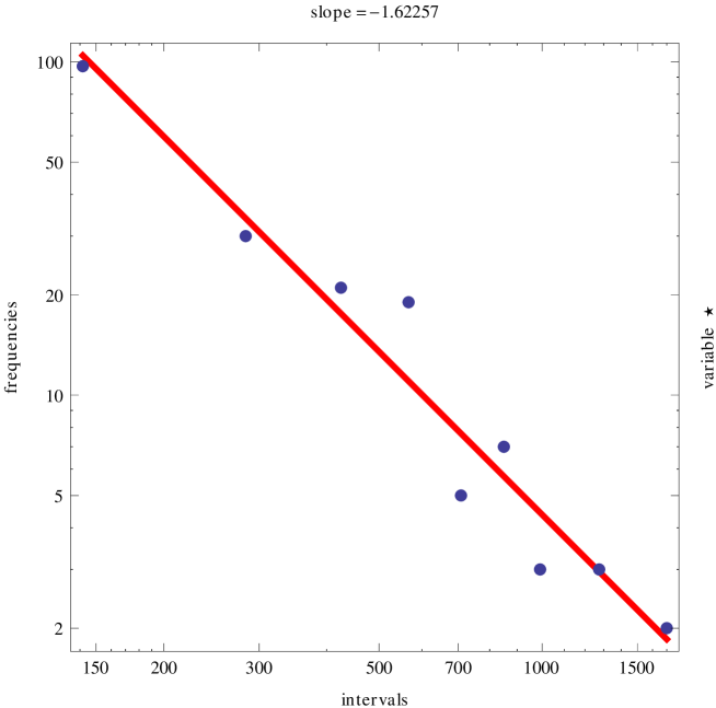
Figure 2: The frequency of the intervals of fixed polarity. The distribution is very roughly fitted by a power law with the index -1.6.

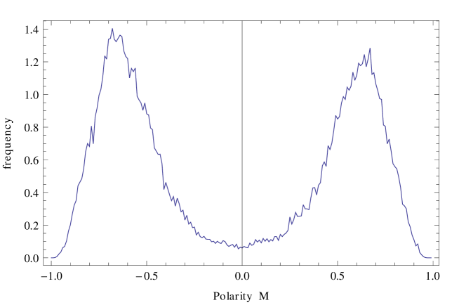
Figure 3: The total frequency distribution of $M\left(t\right)$. The left-right symmetry, or the symmetry in normal-reversed polarites, is not respected. This indicates the model has strong fluctuation in the long time variation. This accord with the ever increasing power spectrum toward low frequency region Fig.(1).

The apparent asymmetry in Fig.(3) is not caused by the initial condition but suggests long range temporal fluctuations in our model. This seems to be consistent with the ever increasing power spectrum in the low-frequency direction in Fig.(1).

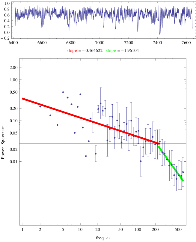
Figure 4: (top) A typical time series of $M\left(t\right)\equiv\vec{\Omega}\cdot\vec{M}\left(t\right)$  in some chron. The valuea are mostly negative but perpetually fluctuating strongly. (botom) The power spectrum of this time series. The data is sucessfully fitted by the the two power laws with the indeces -0.46 for low grequency and -2.0 for high frequency regions.

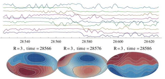
Figure 5: (top) Individual spin motion around a typical polarity flip at time 31264. Vertical axes represents $\vec{\Omega}\cdot\vec{s}_{i}\left(t\right)$ for each spin with shifted zero points for visibility. The first spin from top was rapidly rotating before the flip but the nineth spin took over this role after the flip. These perpetually rotating spins form the gas phase. See the next section for detail. (bottom) The countour/density graph for horizontal component of the magnetic field Eq.(18) on the earth surface around this polarity flipping era. Each ellipse represents the entire earth surface drown in Mollweide mapping, before, right in the middle, and after the flip from left to right. The radius of the spin ring is assumed to be one-third of the Earth radius.

The results of LCS model for geomagnetism is almost the same as our previous study on SCS model and are not so far from the observational values. Thus the range of interaction is shown to be irrelevant for geomagnetic characteristics. In the SCS model, even the inertial term was not necessary to yield the similar results.

5 General properties of LCS model

It is interesting to notice that this LCS system, we explored in the last section, is a slight extension of the Hamiltonian Mean Field model (HMF (Antoni & Ruffo 1995), (Campa, Dauxois , & Ruffo 2009) by adding the potential term $\mu\sum_{i=1}^{N}\left(\vec{\Omega}\cdot\vec{s}_{i}\right)^{2}$. HMF model a good tool to describes phase transitions and statistical fluctuations of a deterministic system composed from many elements. Slightly modified version of HMF model was applied to describe the self gravitating systems(Sota, Iguchi, Morikawa, Tatekawa, & Maeda 2001). However this HMF model itself cannot describe the polarity flip of geomagnetism because of the lack of the preferred angle. The polarity flip is made possible simply by introducing the above potential term. In this sense our LCS model is the minimal model to describe geomagnetism.

Acute readers might have some concern that the geodynamics is a dissipative system rather than the conservative system like HMF model. However the difference is not relevant in our context. HMF and LCS systems have strong chaoticity and the mean field $M$ has apparent statistical fluctuations. In short, these systems have the relevant central degrees of freedom (i.e. mean field) and the rest (i.e. environmental degrees of freedom) together. We focus on the mean field. The mean field immersed in the rest behaves as the dissipative system. This point will be clarified in the rest of this section.

Dynamics of both HMF and LCS models can be visualized by the interacting $N$-particles which are moving on a circle of unit radius as shown in Fig.(6). This is a typical snapshot of the spin angles $\{\theta_{i}\}\left(i=1...N\right)$ represented by the points on a circle. The whole ring represents all the directions of spins $0\leq\theta<2\pi$ and the top position of the ring is the direction of the earth rotation axes $\vec{\Omega},$ $\theta=0$.

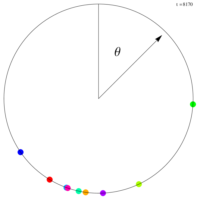
Figure 6: A typical snapshot of the spin angles $\theta_{i}\left(i=1...N\right)$. The whole ring represents $0\leq\theta<2\pi$ and the top position of the ring is $\theta=0$. The earth rotation axes $\vec{\Omega}$ has the fixed angle $\theta=0$. As is shown the most spins are condenced to the almost fixed angle (i.e. fixed polarity), and few rapidly rotating spins exit. The latter trigges the flip of the condensed spins intermittently.

Furthermore it is remarkable that both HMF and LCS models have two classes (phases) of elements: the spins in expanded phase which are almost freely moving all the angle and the spins in condensed phase which are bounded in a localized angle. There exists a critical energy in HMF model in the limit $N\rightarrow\infty$; the condensed phase appears only when the system energy is below this critical energy and the portion of the condensed phase increases for lower energy. Similarly in our LCS model, expanded and condensed phases coexist in wide rage of parameters. We have chosen our parameter so that the system energy is low enough to guarantee that the both phases coexist in one system. The condensed phase yields finite order parameter defined by Eq.(17). Free spins in the expanded phase perpetually disturb the condensed cluster spins and is considered to trigger the intermittent signature change of the order parameter Eq.(17). It is interesting that the expanded and condensed phases often exchange their constituent spins when the angles of the spins coincide with each other, i.e. ‘collide‘ in the above visualization.

In terms of geomagnetism, coexistence of the expanded and condensed phases are essential; the latter yields the well defined polarity in magnetism Eq.(17) and the former triggers the intermittent flip of the polarity. This phase coexistence is naturally realized in LCS model when we choose mildly low energy values. Thus, this model naturally deduces that the system energy required for intermittent polarity flip necessitates the coexistence of the relatively steady component and the rapidly changing component in geomagnetism. The former is of course from the condensed phase and the latter from the expanded phase. Since the macro-spin has magnetic dipole, these freely moving spins in the expanded phase yields rapidly moving pairs of local magnetic spots of reverse polarity superposed on the average steady dipole magnetism caused by the spins in condensed phase. These pairs also have a tendency to align on north-south direction according to the potential form in Eq.(19). These pairs have some similarity with The South Atlantic Magnetic Anomaly (SAMA) observed on the core-mantle boundary (Korte 2010).

The above interpretation that the spins in the expanded phase trigger the flip of the global magnetic polarity suggests that a possible correlation between the activity of the spins in expanded phase and the duration of the fixed polarity. Actually in our numerical calculations, the expanded phase temporally disappears in the superchron, i.e. the longest period of fixed polarity. This correlation should be further studied. Anomalous acceleration in the movement of the local magnetic spots of reverse polarity may predict a polarity flip in the near future.

It is also interesting to notice that this set of equations Eq.(21) is a slight extension of the Kuramoto model for synchronization(Kuramoto 2003, Acebron, Bonilla, Perez, Ritort, & Spigler 2005) by the change of potential: $\mu\sum_{i=1}^{N}\left(\vec{\Omega}\cdot\vec{s}_{i}\right)^{2}\rightarrow-\sum_{i=1}^{N}\omega_{i}\theta_{i}$, and the reduction of the order of time derivative: $\ddot{\theta}_{i}\rightarrow\dot{\theta}_{i}$. The potential $-\sum_{i=1}^{N}\omega_{i}\theta_{i}$ forces each angle $\theta_{i}$ to rotate with the fixed frequency $\omega_{i}$ despite the lack of the inertial term. Therefore the latter simplification $\ddot{\theta}_{i}\rightarrow\dot{\theta}_{i}$ is possible in Kuramoto model. Kuramoto model is a set of long-range coupled oscillators with different frequencies. If there were no interaction between the oscillators, then each phase of the oscillator behaves independently. However if the long-range interaction is sufficiently strong, then the phases of oscillators synchronize with each other despite the difference in each frequencies $\omega_{i}$. Kuramoto model very generally describes the synchronization processes of many type of oscillators and limit cycles including chemical and biological systems.

It is remarkable that LCS model can also describe the synchronization of element spins and yield quasi-periodic motion of the mean field, by simply changing the parameters. The first term of RHS in Eq.(19) gives independent non-linear oscillations of each spin angle. Since the oscillation is nonlinear and the amplitudes are different from spin to spin, the phases of the spins behave very chaotically. The second term of RHS in Eq.(19) gives the cosine potential between all the spin pairs ($\vec{s}_{i}\cdot\vec{s}_{j}=\cos\left(\theta_{i}-\theta_{j}\right)$) and thus naturally yields the tendency for all the pairs to synchronize with each other. Whether the whole synchronization actually takes place or not depends on the balance between the two terms. If the pairwise interaction $\lambda$ is sufficiently large in LCS model, then the synchronization takes place as in the case of Kuramoto model. However, reflecting the strong non-linearity of the cosine potential, the synchronized oscillation becomes quasi-periodic in general. This potential ability of LCS model to describe synchronization physics is especially important when we apply LCS to the solar magnetism in later sections.

6 Other Planets and celestial objects

We would like to argue, in this section, to what extent the LCS model can be general in wider contexts. The concept of the coupled dynamo elements itself, as we have discussed in section 2, is general and is not in principle restricted to geomagnetism. We expect the same for LCS model, which is the minimal realization of this concept. The magnetic fields associated with celestial objects are quite common in the universe; many planets, satellites, and the stars including our Sun. Although the magnetic fields of these objects have variety that is quite different from the geomagnetism, all the magnetic fields are thought to be generated and supported by the robust dynamo mechanism.

However the LCS model is at most a phenomenological model to describe dynamo systems. The LCS model is simply a macroscopic description and cannot be directly deduced from the microscopic MHD equations Eqs.(1-4), which are especially important for quantitative argument in wider contexts. Therefore we need to supplement LCS model with the MHD equations.

First we examine the energy flow for geomagnetism. Geomagnetic fields would be amplified by the inward-winding motion of the convection vortex, anti-cyclone. This inward motion is caused by the Coriolis force induced by the earth rotation although the rotation itself cannot directly transfer its energy to geomagnetism. On the other hand, the convective motion of the iron fluid is supported by the thermal flow from the central region of the earth. This flow is mainly supported by the release of the gravitational potential by the core sinking. Thus the thermal flow accelerates the convective motion and supports the inward-winding force to amplify the magnetic fields through the Coriolis force.

One essential fact for this thermal energy flow is that the main dissipation is due to the Joule heat. This is because the magnetic Prandtl number $P_{m}\equiv\nu/\eta$, i.e. the ratio of the time scale of magnetic diffusion ($1/\eta$) and that of convective diffusion ($1/\nu$), is actually very small: $P_{m}\approx 10^{-6}\ll 1$.

We now closely look at the basic equations Eqs.(1, 3) in the above picture of energy flow. From Eq.(3), we first notice that the steady state for the magnetic field requires the energy balance on average: $\nabla\times\left({\vec{v}\times\vec{B}}\right)+\eta\Delta\vec{B}=0$, which reduces to the relation which is independent of $\vec{B}$,

$$v\approx\left(\gamma\mu_{0}\sigma R_{c}\right)^{-1},$$ (22)

where $R_{c}$ is the Fe-core radius and $\gamma R_{c}$ is the radius of the Taylor cell. The existence of this special scale is essential to our model to characterize the dynamo elements; most of the relevant process of dynamo takes place on this scale. This small scale compared with the core size is foreseen from the order in Eq.(8). The magnetic field is amplified by the inward winding motion of the convection vortex through the term $\nabla\times\left({\vec{v}\times\vec{B}}\right)$ until this steady state Eq.(22) is realized. On the other hand, the inward-winding motion of flow is generated by the term $-2\rho\vec{\Omega}\times\vec{v}$ in Eq.(1), and this term should eventually balances with the backreaction from the generated magnetic pressure through the term $\vec{j}\times\vec{B}$ in the same equation. Therefore in the steady state, we have the estimate of the typical strength of the magnetic field $B_{in}$ at the scale $\gamma R_{c}$, the scale of the Taylor cell, as

$$B_{in}\approx\left(2\rho_{0}\Omega v\mu_{0}\gamma R_{c}\right)^{1/2}.$$ (23)

The observed magnetic field $B_{out}$ at the Earth surface is related with this estimated $B_{in}$ through the magnetic flux conservation as,

$$B_{out}=\left(\frac{\gamma R_{c}}{R}\right)^{2}NB_{in},$$ (24)

where $N$ is the number of Taylor cells in the core and $R$ is the Earth radius. We simply assumed that all the Taylor cell is the same scale and the magnetic fields associated with TC are parallel to the rotation axes of the earth for simplicity. Combining the above three equations, we have

$$B_{out}=N\gamma^{2}\left(\frac{R_{c}}{R}\right)^{2}\left(\frac{2\rho_{0}\Omega}{\sigma}\right)^{1/2},$$ (25)

and the corresponding (virtual) magnetic moment $d$ becomes

$$d\equiv B_{out}R^{3}=N\gamma^{2}R_{c}^{2}R\left(\frac{2\rho_{0}\Omega}{\sigma}\right)^{1/2}.$$ (26)

In the geomagnetic case, we have chosen $N=9$ and putting reasonable values, $R=6357$km, $R_{c}=3480$km, $\sigma=3\times 10^{5}\mathop{\mathrm{S}i}$emens/m, $\rho_{0}=5497$kg/m³, and assuming $\gamma=10^{-1}$, we have $B_{out}=0.4\times 10^{-4}$Tesla from Eq.(25), and $v=7.62\times 10^{-6}$m/$\sec$ from Eq.(22). Although the value of $B_{out}$ is consistent with observations the value of $v$ is only $8\%$ of the estimated speed of the convection flow simply from the west-ward drift motion. If this discrepancy is real, the time scale of the magnetic field variation or of the electric current change is about ten times larger than the convective flow speed. This point should be further studied.

The estimate of the effective magnetic moment in Eq.(26) is general since it is deduced simply from the basic equations (1, 3) based on the LCS model. The expression Eq.(26) is consistent with the general claim in the literature (Christensen2010), (Stevenson 2010) that the planetary magnetic fields are essentially determined from the factor $\sqrt{2\rho_{0}\Omega/\sigma}$. We can step further and estimate the unknown factor $N\gamma^{2}$ in Eq.(26). By using various data for celestial objects, but assuming $\sigma$ is a constant, we can draw a graph for $d$ against $R^{3}\sqrt{2\rho_{0}\Omega/\sigma}$. This turns out to show a power law relation with the index about 3/4: $d\propto\left(R^{3}\sqrt{2\rho_{0}\Omega/\sigma}\right)^{3/4}$, though this is not what we needed. Simply motivated by this scaling relation, we can draw a similar graph for $d/(R^{3}\sqrt{2\rho_{0}\Omega/\sigma}M^{1/2})$ against $M$ in Fig.(7). This relation turns out to be almost a constant within a factor $10$ for the whole mass range of 8-digits as shown in Fig.(7).

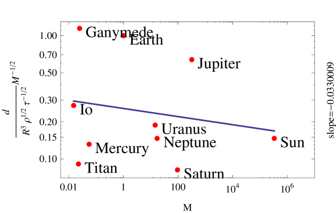
Figure 7: The quantity $d/(R^{3}\sqrt{2\rho_{0}\Omega/\sigma}M^{1/2})$ is shown in the vertical axes against the mass $M$ in the horizontal axes for various celestial objects. These quantities are normalized by the values of earth. The data are from Stevenson (2010). Eulopa and Callisto are excluded from the figure because their magnetic fields are probably induced from the external fields (Stevenson 2010). The value $4\times 10^{-4}$T is used for the solar dipole magnetic field. The quantity $d/(R^{3}\sqrt{2\rho_{0}\Omega/\sigma}M^{1/2})$ turns out to be an almost constant within a factor $10$ for the mass range over 8 digits. This fact suggests the scaling $N\gamma^{2}\propto M^{1/2}$, which determins the number and the radius of the dynamo element in general.

The factor $M^{1/2}$ is important for this constancy. We can deduce the scaling formula, from this phenomenological relation, as

$$N\gamma^{2}\propto M^{1/2}.$$ (27)

In other words, the scaling Eq.(26) holds if we choose Eq.(27). This phenomenological scaling is helpful to reveal the number of dynamo elements. For example, if we suppose the parameter $\gamma$ is almost a constant for various objects, and $N=9$ for Earth, we have $N=9\times(M_{\odot}/M_{\text{earth}})^{1/2}\approx 5\times 10^{3}$ for the sun. However, we must keep in mind that the planets, satellites and stars are very different with each other and the structure of dynamo mechanism is different (Stanley 2010) despite the above generality.

Keeping the above caution in mind, it is interesting to try the unified view of planetary magnetism within our model. In the context of the LCS model, observed large dipole tilt more than $50^{o}$ and the quadrupole moment of magnetic fields in Uranus and Neptune are not exceptional. The magnetic field described by LCS model naturally becomes irregular and asymmetric when occasional large excursion takes place. We may observing these irregular and asymmetric fields in the present Uranus and Neptune. Moreover in the context of LCS model, almost axis symmetric magnetic field of Saturn does not conflict with the anti-dynamo theorem, which inhibits dynamo function in  the axisymmetic steady configuration. This is because individual element dynamo yields magnetic field independently from others and easily violates axis symmetry of the whole system. The magnetic field in LCS model is rapidly changing and steady condition is also violated.

7 Application of LCS model to the solar magnetism

As we have seen in the previous section, a simple argument on the MHD equations based on the LCS model can yield a general scaling law for planets and satellites. This was useful to estimate the scale of dynamo elements. In this section, we would like to explore this generality of the LCS model by applying it to the solar magnetic dynamics.

LCS model does not specify the macro-spin or dynamo element. The macro-spin can express any subsystem which has minimal dynamo property. Typically the element is the inward-winding vorticity. In case of our sun, the macro-spin may be the convecting vortex deep inside the solar surface. It may happen that this region is turbulent and the hierarchy of vortices yield a network of many dynamo elements. The very end of this hierarchy may appear on the entire surface of the sun, possibly as the supergranulations. Recently the pattern of the supergranulation is observed by using the local helioseismology (Nagashima 2010). On top of these supergranulation, strong horizontal magnetic field is observed everywhere on the surface (Ishikawa 2008). We speculate that these vortices associated with dynamo function may fill the entire convecting region inside the sun.

The solar magnetism changes its polarity quasi-regularly with the period about 22 years, which synchronizes with the solar activity of period 11 years. The solar activity can be roughly measured simply by counting the sunspots (SIDC 2011). We show this daily count profile in Fig. (8) top, during the past two hundred years. The power spectrum, shown in Fig. (8) bottom, reveals the clear periodicity of about 11 years, as well as the period of about a month. The latter period is an artifact reflecting the systematic sunspot change on the solar surface which rotates with this period. What is interesting for us is the scaling property with index $-1.1$, near to $-1$, on top of the two peaks associated with the above periods. One-over-f noise or the pink noise, i.e. its power spectrum scales with index $-1$, has been observed everywhere in nature. (For a comprehensive list of references on 1/f noise, see (Li 2011)). Similar 1/f noise in the monthly averages of the sunspot numbers has been reported in the high frequency ($f>\left(11\text{year}\right)^{-1}$) regions (Franchiotti, Sciutto, Garcia, & Hojvat 2004).

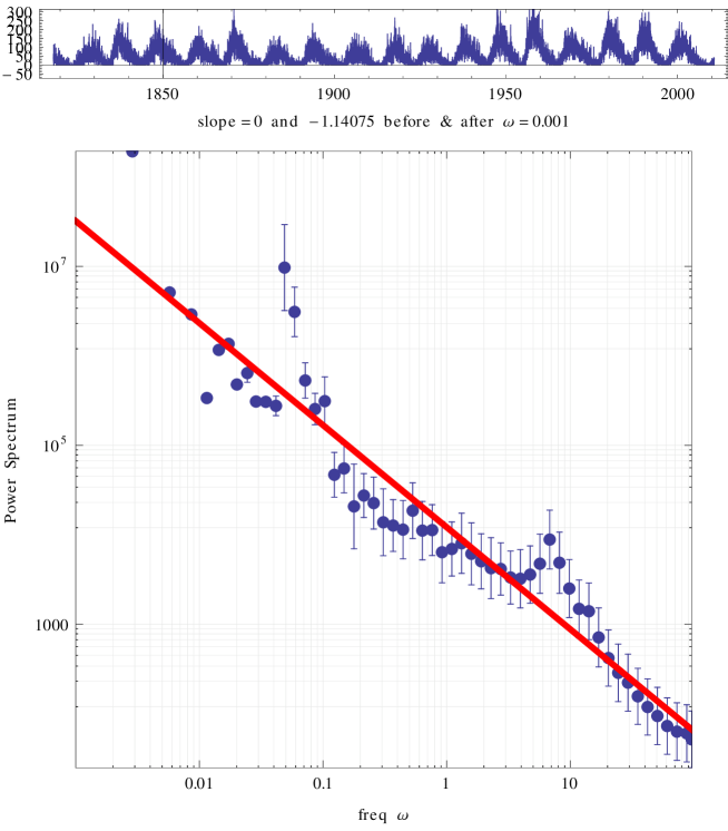
Figure 8: (top) Dayly number of sunspots are shown in the vertical axes against the time in year in the horizontal axes. (botom) The power spectrum of this time series. The data is sucessfully fitted by a power law with the index -1.1 on top of the two peaks at $\omega\approx 0.05$ and $\omega\approx 7$. The former peak corresponds to the 11 year solar activity cycle and the latter peak fictitiously appears corresponds to a month the solar rotation period.

It is remarkable that the LCS model shows quasi-periodic polarity flip, which resembles the solar magnetism, as a result of synchronization of many spins. For the synchronization process to set in, we need large number of spins ($N\gg 1$) and low potential barrier ($\left|\mu\right|\ll 1$). Then the spins in LCS model can naturally synchronize to yield quasi-periodic motion like in the Kuramoto model.

For example in a numerical demonstrations, we set $N=101,$ $\mu=-0.01,$ $\lambda=-2$, and obtained the result as shown in Fig.(9). The top figure shows the time evolution of the order parameter $M\left(t\right)\equiv\vec{\Omega}\cdot\vec{M}\left(t\right)$ defined in Eq.(17). Quasi-periodicity in its evolution is apparent. The amplitude irregularly varies and even becomes almost flat in some periods. The bottom figure shows its power spectrum. Beside the apparent peak corresponding to the quasi-periodicity, one-over-f noise, actually the power $-0.85$, is observed in low frequency region. However this result needs to be refined before serious discussions. For example, the number of spins $N=101$ is apparently too small compared with the previous estimate $N\approx 5\times 10^{3}$ in the last section.

If we suppose that the solar magnetic activity is linked with the number of sunspots, then the above results suggest that the LCS model can reproduce the observed solar activity especially the quasi-periodicity as well as 1/f like power law in the low frequency region in its power spectrum.

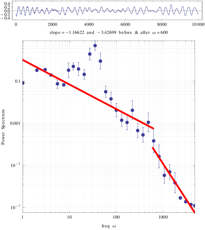
Figure 9: (top) A typical time series of $M\left(t\right)\equiv\vec{\Omega}\cdot\vec{M}\left(t\right)$  in the numerical calculation with the parameter $N=101,$ $\mu=-0.01,$ $\lambda=-2$, and the initial condition is chosed so that all the spin angles are equally separated within the 70% of the whole angle $0\leq\theta<2\pi$. Each spin has the interaction with nearest $10$ spins. The quai-periodic oscillation is apparent. This oscillation appears as a result of synchronization of many spins. (botom) The power spectrum of this time series. There is a peak at $\omega\approx 30$ reflecting the above quasi-periodicity on top of the rough power law behavior with index $-1.2$ in low frequency region. These behaviors accord with the solar observation in the previous figure.

8 Summary and Discussions

We have developed a long-range coupled macro-spin LCS model for geomagnetism, solar magnetism, and others. We have seen this model is minimal and general.

In section 2, we developed the idea of the coupled dynamo elements for general dynamo mechanism in magnetohydrodynamical systems such as geomagnetism. The element should have inward-winding vorticity to amplify the magnetic fields. The we introduced a macro-spin representing such element. In section 3, we have reviewed the short-range coupled spin (SCS) model which successfully describes geomagnetism. In section 4, we introduced the long-range coupled-spin (LCS) model which also successfully describes geomagnetism. Thus the spin models are shown to be useful to describe geomagnetism in the context of statistical fluctuations.

In section 5, we studied the physical relevance of LCS model. First of all in this model, two phases of spins can coexist: The expanded phase in which the spins can rapidly move all the directions almost freely and the condensed phase in which the spin directions are bounded into narrow region to form the dominant dipole moment which is almost steady. The spins in expanded phase perpetually ”collide” (see the figure 6) with the condensed phases and trigger its intermittent polarity reversal. On the other hand LCS model shows quasi-periodicity as well as 1/f noise on top of it. This is the synchronization of the constituent spins. In both cases, the system shows power law behavior reflecting the long range interactions. The phase coexistence is essential for geomagnetism and the synchronization for solar magnetism. These study taught us how the general models such as Hamiltonian mean field (HMF) model and Kuramoto model, if slightly modified, can describe the universality and variety of general dynamo mechanism.

In section 6, we applied LCS model, supplemented with MHD equations, to other planets and satellites. Finding a useful scaling low, we could estimate the scale and the total number of the dynamo element, or macro-spin, in terms of the mass $M$ of the body. In section 7, we applied LCS model, with different parameter values, to the solar magnetism and successfully describe the quasi-periodic oscillation of the solar magnetism on top of the 1/f noise property in low frequency regions. Thus we have actually demonstrated the universality and variety of LCS model.

Although the LCS model can describe most of the geomagnetic observations, it cannot be deduced from the basic MHD equations. It is also possible to generalize LCS model to endow each spin with dynamo function. This is realized for example by setting the homopolar generator (Faraday disk) for each dynamo element, $(1\leq i\leq N)$, and introduce appropriate interactions between them. This is an extension of the original Rikitake model (Rikitake 1957).

If we introduce nearest neighbor interaction, we obtain the short-range coupled Rikitake model (SCR), for the currents $\left\{J_{i}\right\}_{1\leq i\leq N}$ and rotation angles $\left\{\omega_{i}\right\}_{1\leq i\leq N}$,

$$\frac{dJ_{i}}{dt}=-J_{i}+\omega_{i}J_{i+1},$$

$$\frac{d\omega_{i}}{dt}=c-\lambda J_{i}J_{i+1}.$$ (28)

We can obtain the occasional polarity flip and power law power spectrum also in this model. However even $N=8$ case, the time evolution of SCR model inherits chaotic spiky profile from the original Rikitake model. The long-range coupled version of Rikitake model (LCR) is also possible,

$$\frac{dJ_{i}}{dt}=-J_{i}+\omega_{i}\bar{J},$$

$$\frac{d\omega_{i}}{dt}=c-\lambda J_{i}\bar{J},$$ (29)

where $\bar{J}\equiv\sum_{i=1}^{N}J_{i}/N$ is the mean field. In this case we obtain a regular and spiky oscillation due to the strong synchronization of the elements. We have not yet performed a full parameter study. Further extension of such models would be possible and they will be worth extensive research.

References

- (1) Acebron, J. A., Bonilla L. L., Perez, C.J., Ritort F., Spigler R., 2005, Reviews of Modern Physics, 77, 137. (http://scala.uc3m.es/publications_MANS/PDF/finalKura.pdf)
- (2) Antoni M., Ruffo S., 1995, Phys. Rev. E52, 2361
- (3) Blackett, P. M. S, 1947, Nature, 159, 658
- (4) Campa A., Dauxois T., Ruffo, S., 2009, Phys. Rep., 480,57
- (5) Christensen U. R., Space Science Reviews, 152, 565
- (6) Dias V. H. A., Franco J. O. O., Papa A. R. R., 2008, Brazilian Journal of Physics, 38, 1
- (7) Fanchiotti H., Sciutto S. J., Garcia C. C. A., Hojvat C., 2004, Fractals, 12 405
- (8) William G., 1600, De Magnete (About the Magnet). Tr. 1893 from Latin to English by Mottelay P. F., Dover Books
- (9) Inglis D. R., 1981, Rev. Mod. Phys. 53-3, 481
- (10) Ishikawa, R., Tsuneta, S., Ichimoto, K., Isobe, H., Katsukawa, Y., Lites, B. W., Nagata, S., Shimizu, T., Shine, R. A., Suematsu, Y., Tarbell T. D., 2008, A&A, 481, L25
- (11) Kageyama A., Sato T., 1997, Physical Review, E55, 4617.
- (12) Kageyama1 A., Miyagoshi T., Sato T., 2008, Nature, 454, 1106
- (13) Kida S., Kitauchi H., 1998, Prog. Theor. Phys., 130, 121
- (14) Kono M., Roberts P., 2002, Rev. Geophysics, 40, 4-1.
- (15) Korte M., Holme R.,,2010, Physics of the Earth and Planetary Interiors, 182 179
- (16) Kuramoto Y., 2003, Chemical Oscillations, Waves, and Turbulence, Dover Publications
- (17) Landau L. D., Pitaevskii L. P., Lifshitz E. M., 1984, Electrodynamics of Continuous Media, Second Edition: Volume 8 (Course of Theoretical Physics), Butterworth-Heinemann. Section 55.
- (18) Li W., 2011, http://www.nslij-genetics.org/wli/1fnoise/
- (19) Lisle J. P., Rast. M. P., Toomre J., 2004, ApJ, 608, 1167
- (20) Matuyama M., 1927, Japanese Journal of Astronomy and Geophysics, 4-3, 121
- (21) Mazaud A., Laj C., 1989, Earth and Planetary Science Letters, 92, 299
- (22) Mori N., Schmitt D., Ferriz-Mas A., Wicht J., Mouri H., Nakamichi A., Morikawa M., 2011, will be submitted.
- (23) Nagashima K., 2010, Ph.D. Thesis, Grad. Univ. for advanced studies [SOKENDAI].
-
(24)
Rikitake T., 1957, Bulletin of the Earthquake
Research Institute, 34-4, 283.
(http://repository.dl.itc.u-tokyo.ac.jp/dspace/bitstream/2261/11863/1/ji0344001.pdf) - (25) Roberts P. H., Glatzmaier G. A., 2000, Rev. Mod. Phys., 72, 1081
- (26) Seki M., Ito K., 1993, J. Geomag. Geoelectr. 45, 79
- (27) SIDC, 2011, http://sidc.oma.be/ daily sunspot numbers from 1812.
- (28) Sota Y., Iguchi O., Morikawa M., Tatekawa T. Maeda K., 2001, Phys. Rev., E64, 056133
- (29) Stanley S., Glatzmaier G., A., 2010, Space Science Reviews, 152, 617
- (30) Stevenson D. J., 2010, Space Science Reviews, 152, 651
- (31) Tsinober A., 2007, Magnetohydrodynamics, 80, 223